
Submitted:
10 November 2026
Posted:
18 November 2026
You are already at the latest version
Abstract
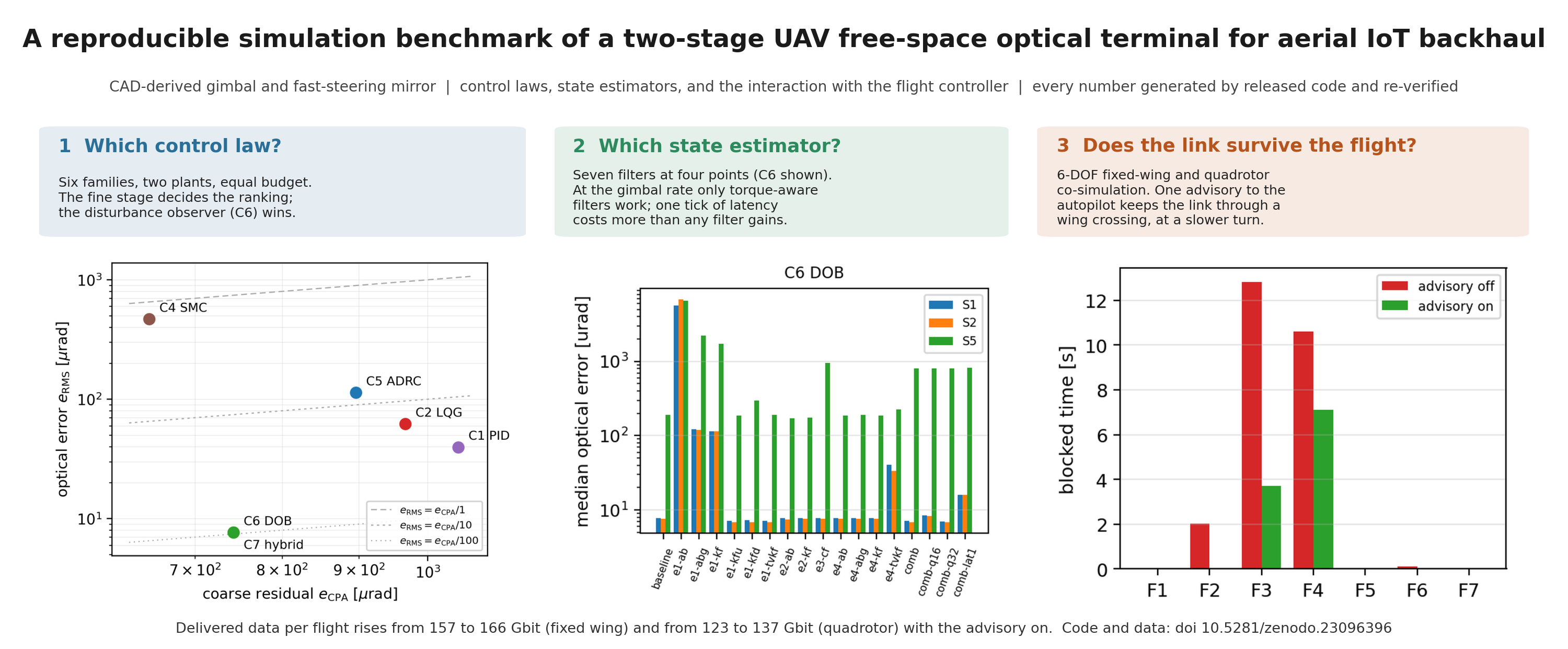
A small unmanned aircraft that collects data from ground sensors and relays it by a free-space optical link is a backhaul node of an aerial IoT network, and its pointing terminal must hold a laser beam to a few microradians while the aircraft moves and blocks part of its own sky. This paper reports one simulation benchmark that answers three questions: which control law to run on the terminal’s two stages, which state estimator at each of its four estimation points, and whether the link survives the manoeuvres a flight controller flies. The terminal model is built from a CAD-derived gimbal and a datasheet fast-steering mirror. Six control families are tuned under an equal budget and compared on two plants; seven estimator variants are compared at fixed control, including embedded costs; and the terminal is co-simulated with fixed-wing and quadrotor models and their autopilots, with a field-of-regard advisory to the autopilot. The disturbance-observer family wins on both plants because the fine stage decides the ranking; at the gimbal rate only filters that know the motor torque are usable, and one tick of latency costs more than any filter gains; the advisory keeps the link through a wing crossing on every seed at the cost of a slower turn, and a tilt limit does the same on the quadrotor at the cost of speed, raising the data delivered per flight.
Keywords:
Internet of Things
; aerial backhaul
; free-space optical communication
; pointing
; acquisition and tracking
; unmanned aerial vehicle
; gimbal control
; Kalman filter
; optical receivers
; system integration
; flight simulation
1. Introduction
A free-space optical (FSO) link from a small unmanned aerial vehicle (UAV) offers data rates that no radio of the same mass and power can match, and asks in return for a pointing accuracy that no airframe can supply on its own: a beam of a few hundred microradians must be held on a receiver kilometres away while the aircraft vibrates, turns and hides part of the sky behind its own wings, tail, rotors or legs [1,2,3,4,5]. The pointing error of a hovering or manoeuvring platform is the term that dominates the link budget of such systems [6,7,8], and the standard answer is a two-stage terminal: a coarse gimbal that carries the optics and follows the line of sight, and a fine stage—here a fast-steering mirror—that removes the residual the gimbal leaves [9,10,11,12]. The recent literature treats the two stages largely apart: the gimbal as a line-of-sight stabilisation problem with disturbance observers and sliding modes, most recently with fixed-time and acceleration-based observers [13,14,15,16,17,18,19,20], and the mirror as a precision-mechatronics problem of hysteresis, resonance and bandwidth [21,22,23,24,25,26,27,28,29]; the review of Dhruv and Kaushal [10] makes the same point for the gimbal side, that the coarse module is the part on which the fine stage’s microradian figures silently depend. Between the aircraft and that terminal sit three engineering choices that are usually made separately and reported, if at all, in isolation: the control law that closes each stage, the state estimators that turn quantised encoders, noisy detectors and a slow navigation solution into what the laws need, and the way the terminal and the flight controller [30,31,32] inform each other so that a manoeuvre does not carry the beam into the airframe. The newest terminal-level work compensates body-pointing uncertainty by feed-forward from the platform’s own motion [33]; this article takes that one step further by letting the terminal talk back to the autopilot.
The setting that motivates the three questions is the aerial IoT network: an unmanned aircraft that flies over ground sensors, collects their data by short radio links and carries or relays it to a station or a second aircraft [34,35,36]. The relay leg is the bottleneck. Radio backhaul from a small aircraft is limited by spectrum, interference and the power a small airframe can spend; the optical link removes all three, at a rate orders of magnitude above the sensor links it serves, provided the beam stays on the receiver [4,37,38]; the line-of-sight stability of UAV relays has become a study of its own [39]. The data such a link delivers is its availability times its rate, and on a manoeuvring aircraft the availability is decided by the pointing terminal and by whether the flight controller cooperates with it; that is what the three questions measure, and Section 3.5 reports the result as gigabits delivered per flight.
This article makes the three choices in order, on one simulation model, with one benchmark protocol, and with each step verified against the one before it. The protocol is the same at every step: the plant is fixed and documented with the origin of every parameter; the alternatives are tuned or configured under an equal budget; the tests are written down before the runs; every table, figure and number is generated by a released script; and an independent script recomputes the quoted numbers from the raw per-run records. Where a test fails, the failure is reported with its numbers rather than the test rewritten.
The contributions are as follows.
- A terminal model built from a CAD-derived gimbal (inertias and the first structural mode from a finite-element solve of the assembly), a datasheet fast-steering mirror and datasheet detectors, with a origin tag on every parameter (Section 2).
- An equal-budget comparison of six control families—PID, LQG, , sliding mode, active disturbance rejection and disturbance observer—on two stages, three operating modes, eight disturbance scenarios and two plants (Section 3.1).
- A comparison of seven estimator variants at the terminal’s four estimation points under fixed control, including the costs an embedded target imposes (fixed-point storage, one tick of latency) (Section 3.2).
- A co-simulation of the terminal with six-degree-of-freedom fixed-wing and quadrotor models and their autopilots, a field-of-regard monitor that predicts the margin to the gimbal limits and the airframe mask from the autopilot’s published intent, and a small advisory message set back to the autopilot, which keeps authority; with the link availability and delivered data per flight that follow, advisory off and on (Section 3.3, Section 3.4 and Section 3.5).
The control laws and filters are standard methods used as published, so their derivations are not repeated; the appendices give what is specific to this study (the design models, the shared signal conditioning, the source and search space of every law and filter, and the gimbal-command geometry the coupling depends on), and the three full reports with all intermediate results are supplied as Supplementary Materials S1–S3.
2. Materials and Methods
Use of generative AI tools. A generative AI assistant (Claude, Anthropic) was used under the authors’ direction to draft and edit the text, to write the simulation code, the analysis scripts and the generators of every table and figure, and to run them; the authors reviewed and verified the output, regenerated every reported number from the released code, and are responsible for the content (see also the Acknowledgments).
2.1. The Terminal: a CAD-derived System Model
2.1.1. Plant Fidelity Levels
Controllers are designed on a linear per-axis model and evaluated on higher-fidelity plants: the nonlinear coarse-axis model with friction and gravity torque, the full terminal with the mirror and detectors, and a flexible-body level that adds the first structural mode. The four levels, their equations and the numerical validation that ties them together are given in Supplementary Report S1; here it suffices that every result below is on the full terminal, and the flexible level is used once, to test the structural-mode prediction.
2.1.2. CAD to Parameters
Figure 1 shows the assembly, names every solid in it and states which moving group each belongs to.
Per moving stage the CAD assembly yields mass, centre of mass and the full inertia tensor about the centre of mass. The elevation assembly is shifted onto the azimuth axis with the generalised parallel-axis theorem, and each tensor is reduced to the scalar axis inertia used by the plant. The pipeline is scripted end to end in FreeCAD, so the reduction is reproducible rather than a spreadsheet step.
Friction, flexible-mode damping, actuator constants and detector parameters are not derivable from a mass-property export, and the toolchain records that fact per parameter rather than absorbing it. Table 1 and Table 2 list the principal parameters, and Table 3 summarises the origin of the whole set.
2.1.3. Multi-rate Schedule
The simulator runs on a base tick: the fine stage and its detector at , the coarse rate loop at , the coarse angle loop at Hz and the line-of-sight and navigation update at Hz (schedule table in Supplementary Report S1).
2.2. The Optical Terminal Model
2.2.1. Line-of-sight Budget
The quantity every controller is judged on is the optical LOS error after the gimbal, the structural mode and the mirror have all contributed:
with for a flat mirror; the small-angle composition used in the kernel is verified against a full rotation-matrix evaluation over the operating envelope. Three features of this budget shape the whole comparison. The factor means the same mechanical performance yields different optical performance at different elevations, so a benchmark that fixed elevation would flatter the coarse stage. The flexible coordinate enters the measured error but is not actuated by either stage: it is the residual no controller can remove. And is why the fine stage is effective at all, but it also doubles any mirror command error. Because the optical error is what is regulated, the fine loop drives the measured error to zero rather than tracking a mirror-angle reference: a mirror servoed to an angle computed from a detector reading inherits every calibration error in that computation, whereas a loop closed on the detector null does not.
2.2.2. Four-quadrant Detector and Link
For a Gaussian spot of radius w centred at the power on an axis-aligned rectangle separates, so each quadrant is a product of error functions,
with the inter-quadrant gap, the finite active area, per-quadrant background, shot and thermal noise, saturation and ADC quantisation integrated explicitly, and the normalised errors from the usual quadrant sums. Two modelling choices proved consequential and are documented in Supplementary Report S1: the detector response is inverted from a calibrated table rather than the small-signal slope (a linear inversion under-reports a large error without bound), and lock detection is referred to the power expected on boresight and background-subtracted (a threshold on the measured sum is cleared by background light alone). Pointing loss at the receiver is with ; after a splitter of ratio the data branch receives , the avalanche photodiode’s signal-to-noise ratio follows the shot-plus-thermal expression with gain M and excess-noise factor F, and outage is declared below a stated ratio. Carrying the pointing error through to power matters because the exponential is steep and rewards consistency over average accuracy: a family with a slightly larger RMS error and a well-behaved tail delivers more mean power than one with a smaller RMS and occasional excursions, which is why results are reported as distributions and tails rather than means.
2.3. Operating Modes and the Six Control Families
2.3.1. The Three PAT Modes
A supervisory state machine selects the reference source and the mirror’s authority; it is evaluated as batched array operations, so an entire Monte-Carlo batch may occupy different modes on the same tick.
- Manual pointing
- The gimbal follows an angle command derived from the navigation solution and the attitude estimate. There is no optical feedback and the mirror is parked; the achievable accuracy is set by navigation and attitude error, which is the floor acquisition must search over.
- Acquisition
- A spiral, raster or Lissajous scan sweeps the uncertainty cone until the detector sum exceeds a detection threshold for N consecutive samples and the estimated spot lies within an acceptance radius; the second test rejects off-boresight stray light, the first rejects single noisy samples.
- Tracking
- The fine stage regulates the measured optical error; the coarse stage follows an inertially stabilised, optically corrected line-of-sight estimate and absorbs the mirror’s low-frequency deflection so that it stays near centre. A confirmed loss of lock returns the terminal to acquisition.
The search cone must cover the navigation error and the attitude-estimate bias, because the gimbal points where its own attitude estimate says; the scan pitch must be the detection acceptance window, not the detector’s physical field (Supplementary Report S1).
2.3.2. Coarse-Loop Architecture
The coarse loop is inertially stabilised (Figure 3): the terminal maintains a target-LOS estimate in inertial space, corrects it slowly from the optical error plus the mirror’s low-passed deflection, and commands at the rate-loop rate, with the measured body rate fed forward. Correcting the gimbal angle directly by the optical error instead can act only at the optical update rate, and the platform motion between updates lands on a detector whose linear region is about a milliradian wide.
2.3.3. Controller Families
All six families implement one interface and receive the same signals: a quantised encoder angle (or the detector-derived error for the fine stage), a shared filtered-difference rate estimate, the reference, a feed-forward term and the same actuator limits. No family is given the true state. In one line each (sources, design models and search spaces in Appendix A, Table A1):
- C1 PID: cascaded position/rate loops with derivative on measurement and integral action on both loops.
- C2 LQG: discrete LQR on the integral-augmented plant with a Kalman filter, both designed at the rate the controller runs.
- C: mixed sensitivity by the two-Riccati central controller [40], synthesised in the sampled-data (w-plane) domain, with every verified on the formed closed loop.
- C4 SMC: with model-based equivalent control and a saturation boundary layer.
- C5 ADRC: third-order extended state observer with bandwidth parameterisation [41] in the current discrete form; the standard observer models the plant as a double integrator.
- C6 DOB: nominal PD plus , with realised as one proper transfer function.
A seventh entry, C7, runs C2 to acquire and C6 to track; it is a composition, not a law, and under the corrected plant C6 acquires as fast as C2, so C7 is dominated by its own tracking branch (Supplementary Report S1).
2.3.4. Fairness
The comparison is only meaningful if the following hold, and each is enforced by construction and covered by tests: one plant realisation per case; one sensor model; identical saturation; delays in the plant interface rather than inside any controller; identical disturbance realisations per seed; one anti-windup rule for every family; and an equal tuning budget of 48 objective evaluations per family on training scenarios disjoint from the test scenarios, with a declared objective over error, effort and control total variation, both stages tuned jointly against the final optical error. A feasibility screen rejects unstable, saturated, chattering or unlocked candidates and any loop whose modulus margin is below on either stage. That last rule was added after it was needed: a time-domain objective scored over short runs cannot tell a fast loop from a marginally stable one, and raising the budget from 12 to 48 evaluations made C2 worse until the screen rejected a fine-stage design with a phase margin under . An equal budget is also not sufficient: what each search is allowed to change matters, and C4’s integral gain, once frozen at an integral time of minutes, is now tuned like every other parameter; the gravity sag it caused was predicted by the boundary-layer formula to within a few per cent (Supplementary Report S1).
Three defects of the warm start were found while chasing the second plant’s results, and each read as a controller property until it was found: estimators that started at zero while the encoder read the pointing angle (a torque-limit kick on the first tick that decided which families lost lock), a start at rest while the platform rotated at up to a radian per second (a rate step on the first tick), and an extended state observer integrated with the measurement held (a bias proportional to the axis rate). All three are fixed uniformly—every estimator initialised from the first measurement, the warm start at the tracking rate, the observer in its current discrete form—and every result below was regenerated with every family re-tuned; the before-and-after table is in Supplementary Report S1. Table 4 reports what each family actually received and how much of it the screen rejected: a family that discarded most of its evaluations was searched in the wrong region, which is a fact about the declared search space, not about the method.
2.4. Where the Terminal Estimates
Table 5 lists the four points with what each currently runs in the control-law benchmark (Section 3.1), and what this study varies.
2.5. The Filter Variants
Seven kinds of filter are compared, each in its published form; Table A2 in Appendix A gives the states, inputs, gain rule and source of each. In one line each:
- V1
- the time-varying Kalman filter (tvkf): predicts the state and its uncertainty every tick and corrects both with the measurement; the most general and the most expensive.
- V2
- the steady-state Kalman filter (kf): the same, but with the gains computed once because the model and the noise do not change; ten multiply-adds a tick.
- V3
- the α-β and α-β-γ filters (ab, abg): V2 for a constant-velocity or constant-acceleration model, with one tuning number; the latter is the extended state observer of Section 3.1 under another name.
- V4
- the filter with the torque input (kfu): V2 that also knows the torque the controller applied, so that only the unexplained motion is treated as noise.
- V5
- the Kalman filter on the line of sight (kf at E2): a two-state filter on the optical line of sight and its rate, with the navigation rate as a known input.
- V6
- the disturbance-augmented filter (kfd): V4 with a third state for the torque that must be acting; identical in structure to the extended state observer.
- V7
- the complementary filter for attitude (cf): the gyro integrated and pulled toward the AHRS solution at a stated corner frequency.
The tables use the code names in parentheses; the present filtered difference is diff, the fixed line-of-sight estimate fixed and the attitude taken as published given. What they have in common, what they cost, and the four rules that keep them well behaved on an embedded processor are in the next section.
2.6. Running the Filters on an Embedded Processor
Four rules decide whether a filter that works in double precision on a workstation works in a microcontroller at .
Precompute what does not change. A steady-state filter has no covariance to propagate; its gains are two or three constants. Every candidate that can be run as V2 or V3 should be, and the time-varying V1 reserved for the two places that need it.
Never form alone. The Joseph form (Table A2) costs a few more operations and keeps P symmetric and positive; for more than three states the UD factorisation [42] propagates and never forms P at all, which is what keeps a long-running filter from losing positive-definiteness in single precision.
Scalar updates. Every measurement in this terminal is scalar or a pair of independent scalars (the two detector axes), so no filter needs a matrix inverse: the update is a division by and a scaled subtraction. This is what makes an filter possible on a core.
Fixed point where the range is known. The encoder angle, the rate and the detector error all have known ranges; the covariance does not. The benchmark therefore emulates Q15 and Q31 storage of the estimator states over declared full-scale ranges ( for angles, rad/s for rates, mrad for the mirror-referred error), with the arithmetic in float and any covariance in float, and measures what the storage precision costs (Section 3.2).
Table 6 gives the operation count and the memory of each variant at each point, counted from the recursions in the released code and from the state dimensions in Table 5. These are counts, not timings. Table 18 adds the measured time of one batched step of each implemented variant on the reference machine, which is a Python/NumPy timing and therefore an upper bound on the relative cost, not an embedded timing.
At the most expensive fine-stage candidate needs well under one per cent of a core’s tick; the cost that matters is latency, since one tick at that rate is of phase at and about at the where the best fine loop crosses over. Every candidate is implemented in the current-estimator form (correct with this tick’s measurement, then predict), which has no such delay; the latency condition of the benchmark adds one tick back on purpose.
2.7. The Co-Simulation with the Flight Models
Figure 5 shows the pieces and what passes between them. Three things are new on the aircraft side and two on the terminal side. The flight model is a rigid body with six degrees of freedom (north-east-down position and velocity, a unit quaternion for the attitude, body rates) with the linear-plus-stall aerodynamics of Stevens et al. [43] and Beard and McLain [44] and the coefficients of a small fixed-wing UAV of the 10–25 class, integrated by fourth-order Runge–Kutta at ; the terminal’s base tick is , and the attitude, rates and references are linearly interpolated between flight steps so that the optical error sees no staircase. The autopilot is the conventional cascade—attitude at , heading commanding bank, altitude commanding pitch, airspeed on throttle, guidance at —with gains from successive loop closure [44] and a roll-command rate limit of /. The navigation model gives the monitor a navigation solution ( horizontal and vertical position noise, / velocity noise, held at ) rather than the true pose; the terminal’s own line-of-sight estimate carries the navigation bias, drift and noise of the benchmark scenario model and its attitude the AHRS error model, so each side sees navigation error where it would in flight, and the truth is used only in the exact geometry that decides whether the beam is blocked. The geometry block turns the two navigation solutions and the attitude into the line of sight, its rate, the gimbal command and the rate feedforward (Section 2.8); the field-of-regard monitor predicts the margin to the gimbal limits and the airframe mask over a horizon and derives the advisory (Section 2.9 and Section 2.11). The link partner is a fixed ground station or a second UAV on its own autopilot; the optical channel reduces to range loss and the Gaussian pointing loss, so the logged received power is a direct function of the pointing error, and scintillation [45] is represented only by the stored fade series of the sensor-degradation scenario.
2.8. Geometry: from Two Poses to a Gimbal Command
Figure 6 shows the frames. In words: subtract the two positions to get the line of sight in the navigation frame; rotate it by the aircraft’s attitude into the body frame, and by the fixed mounting angle into the gimbal’s base frame; the azimuth and elevation of the resulting vector are the gimbal command. Its time derivative has two parts with clear meanings: the relative velocity of the two platforms, which is slow (a few milliradians per second at kilometre ranges) and comes from the navigation solutions at ; and the body rotation sweeping the line of sight across the gimbal, which is fast (a coordinated turn at / is /) and comes from the gyro at . The earlier benchmarks already feed the second term forward; this design adds the first and states where each comes from (feed-forward of the platform’s own motion is also the route of the most recent terminal designs [33]). Near nadir the azimuth rate is unbounded (the gimbal-lock cone of Section 2.9). The formulas are in Appendix B.1.
How this enters the terminal. The terminal simulator of the earlier benchmarks commands its gimbal to the line of sight minus the yaw and pitch it measures, in the small-angle sense, and knows nothing of roll. The coupling therefore hands it the reference
so that its command is the exact gimbal azimuth of Appendix B.1 up to the attitude-estimate error, with the effect of roll inside it; and the rate reference is the exact gimbal rate minus the body-rate feedforward the terminal already adds, so that the sum the terminal forms is . Two details of that hand-over were found the hard way and are given in Appendix B.2. The terminal simulator has no mechanical stop and no airframe: a direction outside the usable region is made physical by setting the optical fade to zero, so that no light reaches the detectors and the terminal’s own supervisor drops lock and reacquires when the direction returns. The test suite checks that a coupling built from the S1 scenario’s own attitude and line of sight reproduces that scenario’s run bit for bit (Section 2.14).
Timing. The navigation solution is old when it arrives and is held for ; the geometry block therefore propagates forward by the known latency using before forming , and uses the current gyro sample, not the AHRS attitude, for the rotation term of (A7), because estimator latency is what Section 3.2 found most expensive.
2.9. Field of Regard and Its Margin
The field of regard is the set of the beam can use (Figure 16 shows it with the flown tracks). It is the gimbal’s travel box minus the airframe mask—a list of rectangles in measured or computed from the airframe drawing once—minus the gimbal-lock cone near nadir, where the azimuth rate of (A7) exceeds the coarse stage’s rate limit. The terminal studied is a belly gimbal on a small fixed-wing UAV that looks mostly down: travel in azimuth and to in elevation; wing masks at azimuth 50 to either side above elevation; tail masks beyond above ; a propeller mask within above ; and the lock cone below . The margin is the signed distance in degrees to the nearest edge of the usable region, positive inside, and the monitor’s threshold is .
The monitor computes, at , the required direction now and at points over a horizon , one point per , by propagating the link partner with its velocity and the aircraft through the wind triangle: the heading turns at the coordinated-turn rate of the bank the autopilot intends, until the commanded course is reached, and the ground track is the airspeed along the heading plus the wind, taken as the difference between the ground velocity and the airspeed along the present heading. When the coordinator (the state machine of Section 2.11, which turns the monitor’s margins into an advisory) weighs alternative manoeuvres it extends the horizon to the whole turn each alternative implies, plus two seconds; a five-second window cannot tell a good way round from a bad one when the turn takes fifteen. For each point it computes the signed distance to the nearest edge of the usable region, positive inside, in degrees. The margin is
the smallest margin over the horizon and the time until the margin is first violated. Both are logged and both drive the coordination logic.
2.10. Interfaces between Terminal and Autopilot
Table 7 lists what the terminal sends; the data the autopilot provides (attitude and rates at , navigation at , the partner’s navigation, the intent at and a shared clock) are tabulated with their latencies in Supplementary Report S3. Three choices are deliberate. The autopilot publishes its intent (commanded heading, bank and heading rate), not only its state, because the monitor’s horizon prediction is only as good as its knowledge of what the aircraft is about to do. Every message carries the time of its sample, because the geometry block propagates by measured latency rather than by an assumed one. And the advisory carries an urgency level, so that the autopilot can weigh it against its own constraints: level 0 is information, level 1 asks for a heading preference the guidance layer may blend, level 2 says the link will be lost within and asks for the bank limit to be applied now. In the message set of a common autopilot protocol [30] the inputs are existing attitude and position messages and the two outputs are two small custom messages; nothing about the design depends on that protocol.
2.11. Coordination Logic
Figure 7 is the whole logic on the terminal side. It has four states (the fourth, BLOCKED, is entered when the direction is outside the usable region now) and three numbers: the minimum margin , the reaction time the autopilot needs to change heading by the amount the advisory asks, and the hysteresis. The advisory is computed in WARN and URGENT as follows.
What is judged. The state machine judges the flight plan: the course the guidance layer wants and the bank the autopilot would use to reach it, not the command as already modified by an accepted advisory. Otherwise an accepted advisory would clear the warning that produced it, be withdrawn, and the two sides would chatter; the first version of this logic did exactly that, and the trace is in the repository’s history.
Choosing the advisory. In WARN and URGENT the coordinator evaluates the few alternatives an autopilot could accept on the same prediction, each over the whole turn it implies: the commanded turn; the same course change the other way round; the commanded turn at a bank limit of 20 and of . When no turn is commanded, it evaluates a course change of and instead. The alternative with the largest minimum margin becomes the advisory, if it beats the plan by at least ; otherwise the plan stands and the advisory carries only the warning. A course preference, once issued, is held for three seconds so that the autopilot’s blend does not chase a flickering suggestion. A bank angle moves the required elevation by about , which is why a bank limit is the alternative that clears a wing mask and why banking towards a partner inside an orbit is harmless (Section 3.3).
Autopilot arbitration. Four rules, in one function of the released code. (1) A turn-direction preference is accepted if the extra turn it costs is at most , and always at urgency 2. (2) A bank limit is accepted at urgency 2 if it leaves the aircraft able to turn at all (at least ). (3) A course preference is blended, with , and never replaces the flight plan’s course: where the aircraft goes is the autopilot’s, how it turns is negotiable. (4) An accepted turn direction is held until that turn is complete or the plan changes, so that the advisory cannot be withdrawn by its own success; the bank limit is re-evaluated every tick and lifted as soon as the plan is clear again, so that the aircraft banks gently only while the wing is in the way. Every advisory is counted as accepted, blended or overridden, and the count is reported.
2.12. Benchmark Protocol for the Control Laws
The matrix is predeclared as six run series (the word stage is reserved for the coarse and the fine stage of the terminal). Series A is the nominal comparison; Series B varies the disturbance; Series C is a paired Monte Carlo over plant uncertainty; Series D sweeps the optical design; Series P and Q measure manual pointing and cold-start acquisition. Scenarios cover slow attitude tracking (S1), broadband vibration with attitude, structural and rotor bands (S2), an aggressive manoeuvre (S3), gusts (S4), sensor degradation (S5), parameter uncertainty (S6), fades and blockages (S7), a cold-start acquisition case (S8) and continuous scintillation (S10; S9 is the manual-pointing input); the labels are those of the released configuration and are used throughout.
Platform attitude is generated as a -weighted multi-sine. A flat multi-sine over 0.2– implies attitude rates that grow linearly with frequency and exceed the axis rate limit, at which point the benchmark measures the rate limiter rather than the controllers. Target-LOS motion is generated in a separate, slower band: it is geometry, not vibration.
Statistics are paired by seed. We report median and interquartile range, a bootstrap confidence interval that resamples seeds rather than time samples [46], a Friedman omnibus test [47] with Holm-corrected Wilcoxon post-hoc comparisons [48,49] over all fifteen pairs, and the failure probability separately from the conditional performance of surviving runs. Practical-significance thresholds are stated in advance: below 2 % negligible, 2–10 % small to moderate, above 10 % potentially engineering-relevant.
The fixed-step integrator was verified before any comparison was run: a step-size study on the nonlinear coarse plant gives an observed convergence order of 3.36 and an integration error of at the base tick, orders of magnitude below the differences reported below. The two array backends agree (self-consistent). Both numbers are produced by patbench validate.
2.13. Benchmark Protocol for the Estimators
2.13.1. What Is Held Fixed
The plant, the disturbance scenarios, the seeds, the fairness rules and the tuned gains are those of the control-law benchmark (Section 3.1), unchanged, and every run is executed by the same simulator with the estimator selected through one configuration object. The control laws are C6 and C1 with their tuned gains; they are not re-tuned per estimator, because the question is what the estimator changes at fixed control. With the default configuration the simulator reproduces the stored Series A results of the control-law benchmark (Section 3.1) bit for bit, seed for seed; that check is a permanent test in the released code, and it is what makes the numbers of the two benchmarks comparable. Every estimator is initialised as in Section 2.3.4.
2.13.2. The Experiment Matrix
Each estimation point is varied on its own with the other three at their present estimators; then the best variant at each point, chosen by a rule stated before the runs (lowest median optical error for C6 averaged over the two nominal scenarios), is combined; then the combined configuration is run under Q15 and Q31 state storage and under one tick of estimator latency (Table 8). Every cell is run with C6 and with C1 on the slow tracking, broadband vibration and sensor-degradation scenarios, warm start, , eight paired seeds. The present and the combined configurations are additionally run cold, from manual pointing through acquisition, for , to see whether the estimators change how the link is found.
2.13.3. Metrics
For every run: the optical RMS error and its maximum; the coarse residual; the tracked fraction and the number of lock drops; the control effort and total variation; and the estimation error of the varied point against the simulator’s true state—the rate error at E1, the line-of-sight error at E2, the attitude error at E3—as an RMS over the run. For every cell: the median over seeds and the failure probability. For the estimators themselves, apart from any run: the frequency response relative to the ideal derivative, the response to a rate step on the quantised encoder, and the loop each closes with C6.
2.13.4. Tests Written Down before the Runs
- H1
- Replacing the E1 backward difference by any Kalman-type filter changes C6’s median optical error on the nominal scenarios by less than 10 per cent. Rationale: the control-law benchmark (Section 3.1) found the coarse residual dominated by the attitude-estimate error, which no rate estimator touches.
- H2
- On the sensor-degradation scenario, at least one E1 candidate halves C6’s failure probability.
- H3
- At E4, at least one candidate improves C6’s nominal error by more than 10 per cent. Rationale: C6’s fine loop crosses over above with a thin margin, and a cleaner rate estimate there is where the fine stage has the most to gain.
- H4
- At E2, both candidates change C6’s nominal error by less than 5 per cent: the fixed gain of is not what limits the terminal.
- H5
- Q31 storage changes the combined configuration’s nominal error by less than 2 per cent.
- H6
- One tick of estimator latency degrades the combined configuration’s nominal error by more than 20 per cent.
2.14. Implementation and Verification of the Flight Study
The flight study was built in five steps, each verified before the next (Table 9 gives the numbers of the first two): the flight model against its own linearisation (trim residual below 1e-9; an elevator doublet reproduced by the linearised model to 0.5 per cent of peak), the autopilot on the flight model (a turn captured in with the altitude held within ), the geometry against hand-computed cases and a finite-difference check of the rates, the coupling by reproducing the control-law benchmark’s run bit for bit when driven by that benchmark’s own attitude and line of sight (Section 3.1), and only then the monitor, coordinator and arbitration on constructed cases and on the scenarios; the reproduction at the fourth step is what allows a change in the terminal’s numbers to be attributed to the flight.
2.14.1. Scenario Set
Table 10 lists the seven flights: F1 is the control; F2, F3 and F4 each exercise one edge of the field of regard; F5 is the two-terminal case; F6 adds wind and the vibration environment to the turn; F7 is the case a station-keeping terminal flies most. The geometries were chosen on flight-only dry runs, before any run with the terminal in the loop, by scanning station positions with the monitor’s own prediction; the first draft of F2, a turn, ended with the station behind the tail whichever way the aircraft turned, which taught the design that the rear azimuth gap, not the wing, is the dominant mask.
2.14.2. Metrics and Tests Written Down before the Runs
For every run: the time the required direction is blocked; the lead from the first warning to the first blockage; the optical RMS error while the link is usable and locked (the held error); the terminal’s lock fraction, lock drops and reacquisition time; the time from the course command to its capture (the turn time), whose ratio between advisory on and off is the flight-plan cost; and the advisories raised, accepted, blended and overridden. The tests:
- T1
- F1: the link never leaves the usable region and the terminal holds lock for more than 99 per cent of the flight, advisory off or on. A control: if it fails, the geometry or the mask is wrong.
- T2
- F2: with the advisory off the link is blocked on every seed; with it on, at least six of eight seeds are never blocked, and the turn time grows by less than 10 per cent.
- T3
- F3: the first warning precedes the first blockage by at least on every seed, and the blended course preference at least halves the blocked time.
- T4
- F4: the link is lost on every seed with the advisory off and on; advisories are raised, blended or overridden, and none is accepted—the flight plan wins, as designed.
- T5
- F5: no chatter, at most two WARN↔NOMINAL transitions per minute on either terminal, and the link is never blocked.
- T6
- F6: the advisory keeps the link on at least six of eight seeds in wind and turbulence, and the held optical error is within 20 per cent of the estimator benchmark’s S2 result for C6.
- T7
- F7: in the orbit the link is never blocked and no advisory is raised.
2.15. The Same Study on a Heavy-Lift Quadrotor: Airframe, Flights and Tests
A fixed-wing aircraft moves the gimbal by banking. A quadrotor does not bank to turn; it tilts to accelerate, to brake and to hold position in wind, and it can point its nose anywhere without changing its path. The flight study is therefore repeated on a quadrotor carrying a payload, with the same terminal, the same coupling, the same monitor and state machine, and the quadrotor’s own advisory options.
2.15.1. The Airframe, with the Origin of Every Number
There is no published, identified coefficient table for a quadrotor of this class the way there is for the small fixed-wing aircraft; a quadrotor does not need one, because its model has no aerodynamic coefficients beyond a drag area. The airframe is anchored on a manufacturer’s specification sheet for a heavy-lift quadrotor (Freefly Alta X: empty mass, maximum take-off mass and payload, motor circle, propeller, thrust-to-weight ratio, speed and wind limits) [50]. What the manufacturer does not publish—battery and motor masses, motor lag, the reaction torque per unit thrust, the drag area—is assumed and marked so in Table 11, with the check that ties each assumption to a published number: the drag area is the one that gives the datasheet’s maximum speed at a plausible tilt, the thrust ratio is read against the aircraft without payload, and the inertia follows from the stated mass layout. The flying mass with the payload is , hovering at 0.51 of the maximum thrust. The model is a rigid body with four first-order rotor lags, quadratic drag and a PX4-class cascade autopilot (velocity, tilt-limited acceleration, attitude, rate), as released in the code; the stage checks in the lower half of the table verify hover, a / velocity step, a yaw and the hover in the datasheet’s / wind, whose tilt (9.4 against the analytic ) is the quantity that drives the field-of-regard problem.
2.15.2. What Changes in the Design
Three things. The field of regard: a belly gimbal on a quadrotor looks down through a clear lower hemisphere, bounded above by the rotor discs and arms (elevation here), with four landing legs at the arm azimuths blocking shallow views, and the lock cone at nadir. The prediction: the autopilot’s intent is a velocity target, a tilt limit and a yaw command, and the predicted attitude at each point is the tilt that the commanded acceleration plus the drag of the predicted airspeed require, with the commanded yaw; because drag grows with speed, a tilt limit is also a speed limit, and the predictor includes that. The options: the commanded manoeuvre; the yaw the other way round; a tilt limit of 20, 12 or ; and, whenever the plan leaves the heading free, a yaw of or that moves the link away from a leg without changing the path—an option a fixed-wing aircraft does not have. The arbitration accepts a free-heading yaw outright (it costs the path nothing), a tilt limit at urgency 2, and a yaw direction as the fixed-wing case accepts a turn direction. One finding of the fixed-wing study carries over unchanged: yawing cannot change the required elevation, because the tilt is always toward the acceleration and the elevation shift is the part of the tilt that lies along the line of sight, whatever the heading.
2.15.3. Scenarios and Tests
- QT1
- Q1: never blocked, lock above 99 per cent, advisory off or on.
- QT2
- Q2: with the advisory off the link is blocked on every seed; with it on, at least six of eight seeds are never blocked, and the cruise speed the tilt limit allows is at least half the commanded one.
- QT3
- Q3: the first warning precedes the lock cone by at least on every seed, and the free-yaw advisory at least halves the blocked time (it cannot avoid the cone; it can avoid the rear).
- QT4
- Q4: the legs block the link briefly (at most ) and predictably (warned at least ahead), advisory off or on; no option avoids a leg when the yaw must pass it.
- QT5
- Q5: the free-yaw advisory at least halves the blocked time, with at most four WARN toggles per minute.
- QT6
- Q6: never blocked; held optical error within 20 per cent of the control-law benchmark’s S2 result.
- QT7
- Q7: never blocked; the lock fraction is reported against the fixed-wing orbit F7.

Table 12.
The quadrotor scenarios. The aircraft starts at the origin heading north; the station is on the ground; 8 seeds, advisory off and on, the terminal driven through every flight.
Table 12.
The quadrotor scenarios. The aircraft starts at the origin heading north; the station is on the ground; 8 seeds, advisory off and on, the terminal driven through every flight.
| Id | Flight | What it tests |
|---|---|---|
| Q1 | hover at 100 , station 300 ahead, 20 | control |
| Q2 | accelerate to 15 / at 3 , station ahead-right and low (elevation ), 20 | the nose-down tilt lifts the required elevation into the rotor discs |
| Q3 | overflight of the station at 80 , 10 /, 30 | lock cone at nadir, then the station behind |
| Q4 | yaw in hover with the station abeam, 20 | the legs sweep through the line of sight |
| Q5 | two quadrotors crossing, partner 60 below, 25 | the partner starts behind a leg |
| Q6 | hover in a 10 / wind with gusts; terminal in S2, 25 | steady tilt into the wind, vibration in the loop |
| Q7 | orbit of 100 radius, nose to the centre, 40 | continuous tilt and yaw |
3. Results
3.1. Control Laws
3.1.1. Nominal Tracking
Table 13 reports nominal tracking performance. Figure 9 shows the per-seed distributions; a box plot rather than a bar chart of means, because the robustness question is about the tail.
Two features of that table are worth reading carefully, because both are invisible to a benchmark that reports a single end-to-end error.
First, the ranking by final optical error is not the ranking by coarse residual. C4 has the smallest coarse error in the table and the largest optical error of any family that tracks; C1 has the largest coarse residual and the second-best optical error. This is the coarse/fine partitioning question made measurable: a coarse loop only has to keep the line of sight inside the mirror’s range, and effort spent driving it below that buys nothing, while a fine stage that exploits the range it is given can be worth more than a tighter coarse loop. Reporting alongside is what makes the distinction visible; with only the latter, a well-partitioned design and a fine stage compensating for a poor coarse loop look identical.
Figure 8 plots this directly. Distance below a diagonal is the rejection the fine stage achieves, and the families are spread across more than an order of magnitude of it while their coarse residuals span a factor of 1.6. What separates them is mostly what the mirror is doing, not what the gimbal is doing.
Second, one family does not hold lock at all. Its row carries a failure probability of one rather than an error, which is the intended behaviour: a family that cannot track is reported as such and is not quietly omitted, nor given an error statistic computed over the handful of samples in which it happened to be locked. Section 3.1.4 explains the mechanism — its synthesis returns a controller that is itself unstable and is certified only against the linear design model.
Figure 9.
Per-seed distribution of the optical LOS error by controller family and scenario. Each box is the spread over the eight seeds; the dots are the individual seeds, and because the seeds are paired a reader can follow one realisation across every family. A family whose box sits low and short is both accurate and consistent; C4’s long box is its lock losses.
Figure 9.
Per-seed distribution of the optical LOS error by controller family and scenario. Each box is the spread over the eight seeds; the dots are the individual seeds, and because the seeds are paired a reader can follow one realisation across every family. A family whose box sits low and short is both accurate and consistent; C4’s long box is its lock losses.
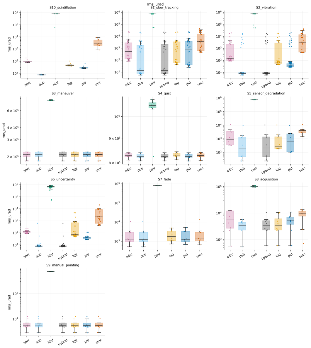
Figure 10.
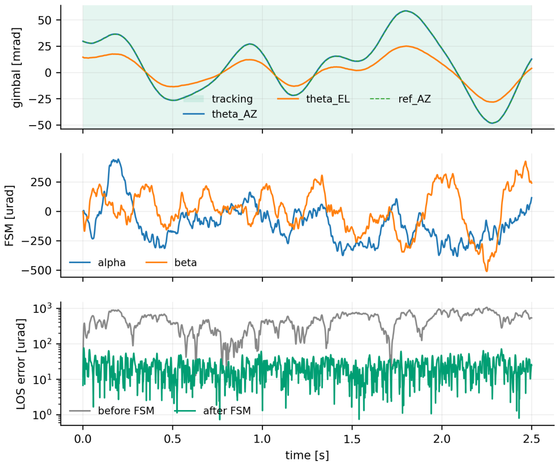
Two-stage decomposition for one run (C1 PID, nominal Series A, scenario S1 slow tracking): gimbal angle and its reference, mirror deflection, and the residual LOS error before and after the fine stage. Background shading indicates the PAT operating mode.
Figure 10.
Two-stage decomposition for one run (C1 PID, nominal Series A, scenario S1 slow tracking): gimbal angle and its reference, mirror deflection, and the residual LOS error before and after the fine stage. Background shading indicates the PAT operating mode.
3.1.2. Transient Response
The tables above are steady statistics and say nothing about how a loop reaches that steady state. Figure 11 answers a step injected by displacing the axis from its reference, on a stationary scenario so that the transient is the loop’s own and not the platform’s.
Three things are visible here that no steady statistic reports. None of the families overshoots: on this plant they are all overdamped, so the classical damping ratio inferred from overshoot is undefined for every one of them, and we report that rather than fitting a second-order model that does not apply. Rise time is nearly uniform for five of the six: they reach 90 of the step within 23 to 25 , which is the acceleration-limited command rather than the loop. C4 alone reaches it in 7 , at the bound the motor’s peak torque and the axis inertia set, because its switching term saturates the actuator where the others follow the profile. What separates the rest is settling, which spans a factor of 4.6 among the families that settle at all, and which does not follow the tracking ranking: C5, fourth on tracking accuracy, settles fastest. A step response and a tracking error measure different things, and a reader choosing a coarse-stage design from one should not expect the other to follow.
C4 then stops about 12 per cent short of the step for the rest of the run, and its elevation axis—which is not stepped—sags. Both are the steady error of a boundary-layer sliding mode under a constant load, , which for the elevation gravity torque predicts 0.33 in the absence of integral action; 0.21 is measured at the end of the run, less than the prediction because the tuned integral term has by then removed part of it. C3 reaches 90 of its step and then loses its elevation axis entirely, by about 31 at the end of the run: the coarse-stage failure of Section 3.1.4 seen in the time domain. Within the run, 5 of the six families settle to ; for C4 the settling column is empty, which is a more honest statement than a number extrapolated past the end of the data.
A correction belongs here. An earlier version of this figure measured the step response as the magnitude of the pointing error over both axes, although only azimuth is stepped. That is harmless while the other axis is quiet, and it is wrong when it is not: C4’s elevation sag was charged to its azimuth step, and because the sag is roughly fixed while the step size is not, it read as a stall at 47 on the step and as a reversal on a quarter-size one. We described that as an amplitude-dependent nonlinearity. It was a constant divided by two different amplitudes. The response is now measured on the stepped axis, with the other reported separately, and the account above replaces the earlier one.
3.1.3. What the Second Stage and the Feed-Forward Are Worth
A removal study that runs every family coarse-only, without feed-forward, and with both stages shows that the fine stage is worth a factor of 5–60 in optical error depending on the family and the feed-forward a further factor of two on the coarse residual; the full table and the seven frequency-domain figures behind it are in Supplementary Report S1. Figure 12 keeps the one that matters: the measured coarse loop of every family; the fine loops, shown in Supplementary Report S1, cross over an order of magnitude higher.
3.1.4. Loop Shaping and the Negative Result (Summary)
The frequency-domain analysis of every executed loop—crossovers, margins, the sensitivity peaks and the Nyquist and Nichols plots of both stages—and the measurement-by-measurement diagnosis of why the family fails are given in full in Supplementary Report S1. Three conclusions from it are used below. First, the fine loop, not the coarse loop, sets the two-stage gain: the families’ coarse residuals cluster while their fine-stage rejections spread by more than an order of magnitude (the factors are in Section 3.1.5), and the optical error is the coarse residual divided by that rejection. Second, a modulus margin below about 0.2 predicts a high failure probability (sliding mode 0.09, ADRC 0.20) and above about 0.45 it stops discriminating; is the exception that proves the margins are not the whole story, with the best modulus margin of all (0.70) and the worst failure rate, because its problem is not a margin but a coarse loop whose gain at is 100 below the others’, so that five per cent of the pointing command survives as steady error; six candidate explanations were ruled out by measurement. Third, the CAD-derived structural mode at (not the first assumed) is 18–28 below every family’s complementary sensitivity, which the flexible-body series confirms.
3.1.5. A Second Plant
One gimbal cannot separate a property of two-stage terminals from a property of this terminal, so the tuning and the nominal series were repeated on a second plant: the reference terminal with its payload mass and both axis inertias doubled and the structural mode scaled accordingly—a scaled variant, so it tests whether the conclusions survive a heavier coarse stage, not whether they hold across architectures; its elevation gravity load is 80 per cent of the motor’s continuous rating. Every family was re-tuned from scratch on it under the same budget in a separate configuration tree. Four tests were written down before it was run (Table 14) and all four pass: the coarse residuals cluster on both plants (spanning factors of 1.6 and 1.4), the fine-stage rejection spreads over factors of 70 and 58, the fine stage accounts for 98.5 and 99.1 per cent of the spread in final error (from , exact for each family), the rank correlation between rejection and final error is and against and for the coarse residual, and the five families that hold lock are ordered the same on the two plants (). The first time these tests were run the last two failed, because of the start-up defect of Section 2.3.4, not the plant; the tests were not altered, and the earlier outcome is kept beside this one in Supplementary Report S1. Three cautions keep the passes in proportion: the second plant is a scaled variant; for C1, C5 and C6 the same search candidate won on both plants; and a rank correlation of one over five families says that the ordering is not fragile, not that it is general.
3.1.6. Disturbance Rejection and Robustness
Under the vibration, gust, sensor-degradation and plant-uncertainty scenarios the ranking of the six families is unchanged, and the disturbance-observer family keeps its optical error within a factor of two of nominal on every scenario except sensor degradation, where all families lose lock on a quarter of the seeds; the per-scenario tables are in Supplementary Report S1.
3.1.7. The Three Operating Modes
Table 15 reports manual-pointing accuracy, time to first lock, lock losses and reacquisition time, the quantities a link-availability budget actually consumes. Acquisition is only weakly predicted by tracking: C1, second on nominal tracking error, is the slowest to reach first lock, taking nearly twice as long as C2 and C6; C6 is both the best tracker and among the fastest to acquire; C4 and C5 reach first lock in reasonable time and then lose it. Tracking rewards a loop that is tight around a small residual, acquisition one that converges quickly from several milliradians with the mirror parked and no optical feedback until detection is confirmed, and a design tuned for the first has no obligation to be good at the second. Manual pointing, the floor both start from, lands within a few per cent for every working family at the milliradian level the acquisition scan is sized to cover (timeline in Supplementary Report S1).
Two further analyses are in Supplementary Report S1: the paired Wilcoxon and Friedman tests with Holm correction, which confirm the ranking at the 0.05 level for every pair except the two leaders on the coarse residual, and the beam-split sweep between the tracking and the communication detector, which shows the tracking error insensitive to the split over a wide range, so that the split should be chosen for the link rather than for the loop.
3.2. State Estimators
3.2.1. What the Estimators Are, before Any Run
Figure 13 (and the rate-step responses in Supplementary Report S2) characterise the rate estimators on their own. Every constant-velocity filter without the torque input (-, --, plain KF) buys its noise rejection with phase: at the where C6’s coarse loop crosses over, the - filter is behind the true rate and the -- filter carries a 4 resonance. The filters that know the torque (KF with input, disturbance-augmented, time-varying) do not pay this: their prediction already contains the motion the torque will cause, and the measurement only corrects the difference. Figure 14 shows what that does to the loop: with the backward difference C6’s coarse loop crosses at with a modulus margin of 0.39; the -- filter leaves 0.05, the - and plain KF 0.17, and the three input-aware filters 0.42 to 0.45. The frequency responses predicted the ranking of the runs before the runs were made, which is the reason to measure them.
3.2.2. The Runs
Table 16 is the whole matrix and Figure 15 draws it; Table 17 gives the tests. 864 paired runs, one simulator, no re-tuning.
E1, the gimbal rate, is where the estimator matters, in both directions. The three filters without the torque input break the loop the frequency responses said they would: the - filter loses lock on every seed of every scenario ( on S1, a limit cycle, not tracking), and the -- and plain KF are fifteen times worse than the backward difference (121.5 and 114.2 against ). This is why H1 fails: it was written on the belief that no rate estimator could change the coarse residual by more than ten per cent, and the belief was wrong for any filter whose bandwidth is set by a noise ratio rather than by the loop. The filters that know the torque go the other way: the KF with input and the time-varying KF improve C6’s nominal error by about ten per cent (-9.8 %, to 7.1 and on S1 and S2), with the time-varying filter converging to the steady-state one within the first milliseconds and giving the same numbers to three digits. The disturbance-augmented filter matches them nominally and is worse when the sensors degrade (299.3 against on S5): its third state absorbs the sensor fault as a torque. None of them halves the failure probability on S5 (0.25 present, 0.25 best), so H2 fails.
A detail worth the reader’s attention: the KF with input has a larger rate-estimation error than the backward difference (51.8 against RMS on S2) and yet points better, while the disturbance-augmented filter has the smallest rate error (26.7) and points no better. The loop does not care about the estimator’s noise; it cares about its phase at crossover. An estimator benchmark that scored estimation error alone would have ranked these the wrong way round.
E2, the line of sight, does not matter. The - tracker and the Kalman filter on the LOS change C6’s nominal error by -1.2 and -0.6 % (H4 passes); on S5 they gain about ten per cent (171.4 and 174.7 against 191.7). The fixed gain of 0.8 at is not what limits the terminal, because the LOS estimate is dominated by the navigation bias the control-law benchmark (Section 3.1) already measured (), which no filter of the optical measurement can see.
E3, the attitude, is the one place where the nominal scenarios mislead. The complementary filter leaves S1 and S2 unchanged (-0.8 %)—it removes the AHRS sample noise, which was never the problem, and passes the AHRS bias, which is (1095 against of attitude error)—and on S5 it is five times worse (949.8 against ), because integrating a degraded gyro toward a degraded AHRS with a two-hertz corner holds the fault for longer than the AHRS alone. Its failure probability is still lower (0.12 against 0.25): it loses lock less often and points worse while locked.
E4, the fine-stage rate, gains nothing and can lose much. The -, -- and steady KF change C6’s nominal error by less than one per cent (H3 fails); C6’s fine loop crosses over above with the present estimator already, and Figure 14 shows the alternatives move the crossover by a few per cent and the margin between 0.17 and 0.31. The time-varying KF is the exception: , five times worse, with 5 less loop gain at low frequency in Figure 14. The reader should treat that loop curve with care: the kernel linearisation differences a filter whose covariance is itself a state, so the curve is the linearisation of a time-varying system; the five-fold error in the runs is not in doubt. For C1 the E4 column is constant to the last digit, because C1’s fine stage does not use a rate estimate at all.
The combination, chosen by the rule written down before the runs, is a lesson about the rule. The rule picked the best nominal variant at each point: tvkf, ab, cf, ab. Combined they give 7.1 and on S1 and S2, the E1 gain and nothing else—and on S5, four times worse than the present set, because the rule admitted the complementary filter on a nominal difference of a tenth of a microradian and paid for it where the sensors degrade. A selection rule that looks only at the nominal scenarios selects for nominal performance.
Embedded conditions. Q31 storage of the estimator states changes the combined configuration’s nominal error by -0.2 % (H5 passes); Q15 by +20 % for C6 and +28 % for C1, which is the quantisation of the rate state over its declared range becoming visible. One tick of estimator latency costs +130 % for C6 (16.1 against ; H6 passes) and +4 % for C1, whose coarse loop crosses over lower and notices a millisecond less. The step responses in Supplementary Report S2 show the same thing in the time domain. Latency is the most expensive thing in this part, by a factor of ten over the best filter’s gain; it is also the cheapest to avoid, because it is a matter of ordering the correction before the prediction in the code, not of arithmetic.
Cold start. The combined configuration acquires no differently from the present one for C6 (first lock at 0.87 against , Table 19); for C1 it acquires faster (1.24 against ) and then fails to hold on 0.25 of the seeds where the present set held all of them. The acquisition results are eight seeds of ten seconds each and are reported as what they are.
Cost.Table 18 gives the operation count and the measured Python step time of every variant. Every implemented filter is within a factor of ten of the backward difference in operations and none approaches one per cent of a tick on a core.
Table 18.
Cost per execution of each estimator: multiply-adds counted from the recursion, and the measured time of one batched step on the reference machine (Python/NumPy, batch of one, median of 2000 calls).
Table 18.
Cost per execution of each estimator: multiply-adds counted from the recursion, and the measured time of one batched step on the reference machine (Python/NumPy, batch of one, median of 2000 calls).
| Point | Variant | States | Mult.-adds | Step time [] |
|---|---|---|---|---|
| E1 | diff | 2 | 4 | 9 |
| E1 | ab | 2 | 6 | 15 |
| E1 | abg | 3 | 9 | 19 |
| E1 | kf | 2 | 10 | 6 |
| E1 | kfu | 2 | 14 | 7 |
| E1 | kfd | 3 | 24 | 13 |
| E1 | tvkf | 2 | 40 | 62 |
| E4 | diff | 2 | 4 | 9 |
| E4 | ab | 2 | 6 | 13 |
| E4 | abg | 3 | 9 | 25 |
| E4 | kf | 2 | 10 | 15 |
| E4 | tvkf | 2 | 40 | 79 |
Table 19.
Cold-start acquisition (S8, 10): median time to first lock and tracked fraction, present estimators against the combined best; the runs are 10 long, so the tracked fractions are not those of the longer Series Q runs of Table 15.
Table 19.
Cold-start acquisition (S8, 10): median time to first lock and tracked fraction, present estimators against the combined best; the runs are 10 long, so the tracked fractions are not those of the longer Series Q runs of Table 15.
| Cell | Law | [s] | |
|---|---|---|---|
| present | C6 | 0.87 | 0.89 |
| present | C1 | 1.57 | 0.83 |
| combined best | C6 | 0.87 | 0.89 |
| combined best | C1 | 1.24 | 0.87 |
3.3. Interaction with the Flight Controller: Fixed Wing
Table 20 is the whole matrix, 112 runs of the terminal through 8 flown flights per cell; Table 21 gives the tests; Figure 16 shows where the required direction actually went. 4 of the seven tests pass. The following goes through the flights in order and says what each one taught, including the three tests that each fail on one clause and the one that passes for the wrong reason.
Figure 16.
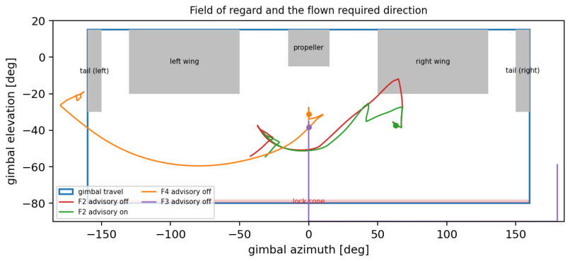
The field of regard with the required direction actually flown in F2 (advisory off and on), F3 and F4. Grey: airframe masks; red band: lock cone; blue box: gimbal travel. Where a track crosses grey or leaves the box, the beam is blocked.
Figure 16.
The field of regard with the required direction actually flown in F2 (advisory off and on), F3 and F4. Grey: airframe masks; red band: lock cone; blue box: gimbal travel. Where a track crosses grey or leaves the box, the beam is blocked.
F1, the control, is clean. On every seed, advisory off or on, the link never leaves the usable region, the terminal holds lock for the whole flight, and the held optical error is —the number of the control-law benchmark (Section 3.1) for this controller on a slowly moving platform. The coupling adds nothing of its own (T1 passes).
F2, the wing crossing, is the case the advisory was built for. Without it, the right wing blocks the beam on every seed for of the banked turn (Figure 17, red; the ground-track figure of Supplementary Report S3); the terminal holds whenever the direction is usable, loses lock the moment the fade goes to zero and reacquires after the wing has passed. With it, the coordinator sees the crossing on the plan’s own prediction the moment the turn is commanded, advises the turn at a bank, the autopilot accepts (urgency 2), banks gently until the plan at full bank is clear again and then rolls to : the link is never blocked on 8 of 8 seeds, lock is 100.0 % and the held error is . The cost is the turn: 12.8 against from command to capture, +65 %. T2 therefore passes its link clause and fails its cost clause (T2 fails); the ten per cent was written before anyone knew that clearing a wing mask means banking at for the first third of the turn, and the number is reported rather than the threshold moved.
F3, the overflight, is predicted early and only partly avoided. Flying straight over the station at , the required direction enters the lock cone at after the first warning on every seed (T3’s lead clause passes: the shortest lead is against the required), and is then behind the tail for the rest of the flight: blocked of 32 without the advisory. With it, the course preference is blended at and moves the track sideways enough to miss the cone: blocked (Supplementary Report S3), which is the halving T3 asked for (T3 passes). Two numbers in this row deserve more attention than the test. The held error is , four times the other flights’, and the lock fraction is well below the usable fraction: at 100–400 range the line of sight moves at up to /, and the terminal’s line-of-sight estimate is refreshed at with a fixed gain, so the reference it follows is a staircase of a milliradian per step. That is the E2 point of the estimator benchmark (Section 3.2), which found no gain from a better LOS filter at kilometre range; at a hundred metres it would find one.
F4, the flight plan that puts the station behind, ends as designed: the aircraft goes where it was told. The link is lost on every seed with the advisory off and on (10.6 and ), because no turn direction, bank limit or thirty-degree course change keeps a ground station inside a field of regard whose rear is masked while the aircraft flies away from it. The autopilot accepted the direction and bank advisories during the turn (0 blended, 188 overridden afterwards) and they bought ; T4 as written also demanded that none be accepted, which was the wrong thing to have written—the arbitration rules accept a harmless bank limit whether or not it saves the link—so T4 fails on that clause while its substance holds: the flight plan wins, and every loss is logged against an advisory that was raised in time.
F5, two aircraft crossing, raises nothing. With of height difference and a crossing, the required direction stays at least inside the region on both terminals and neither coordinator leaves NOMINAL; T5 passes with zero toggles, which is a pass without a trial. The scenario is kept for the symmetric bookkeeping it exercises, not for what it proves.
F6, the turn in wind and turbulence, shows the prediction handling the wind. A / crosswind crabs the aircraft and changes where the wing crossing falls: without the advisory the beam is blocked for (a graze, not the two seconds of F2), and with it on 8 of 8 seeds never (Supplementary Report S3). The held error in the vibration environment is against 7.6 for the same controller in scenario S2 of the control-law benchmark (Section 3.1): 22 more, of which the turbulence and the turn are the difference, and two points outside the twenty per cent T6 allowed (T6 fails on that clause, passes on the link).
F7, the orbit, is safe by geometry and not by the terminal. Banking towards a station inside the circle raises the required elevation by , so the direction never approaches the lock cone (margin ) and no advisory is raised (T7 passes). Yet the terminal holds lock for only 80.2 % of the orbit, with 11 drops while the direction is usable, for the same reason as F3: at 60–210 range the line of sight sweeps at up to a quarter of a radian per second and the fixed-gain LOS estimate cannot keep the fine stage inside its range. The test was written about the field of regard and passes; the flight says the station-keeping case needs a better line-of-sight estimator.
What the four figures add.Figure 16 makes the masks the actors: every loss in the study is a track entering grey or leaving the box, and every save is a track routed round it. Figure 17 shows the advisory’s mechanism in one frame: the true margin (solid) never crosses zero when the predicted minimum (dashed) is acted on. Figure 18 is the whole study in two bars per flight.
3.4. Interaction with the Flight Controller: Quadrotor
The quadrotor of Section 2.15 was flown through Q1–Q7, advisory off and on: Table 22 is the matrix (112 runs) over the flights of Table 12, Table 23 the tests, Figure 19 where the required direction went and Figure 21 the blocked time and held error per flight: all seven pass, and the reader should weigh that against the four of seven of the fixed-wing study before concluding that the quadrotor is the easier platform. It is easier in one respect that the tests reward—a quadrotor can be told to tilt less and to point its nose elsewhere, and both cost the flight plan little—and it is harder in one respect the tests were not written to catch, which the lock fractions show.
Figure 19.
The quadrotor’s field of regard with the required direction flown in Q2 (advisory off and on), Q3 and Q4. The rotor discs bound the region above ; the four grey bars are the landing legs.
Figure 19.
The quadrotor’s field of regard with the required direction flown in Q2 (advisory off and on), Q3 and Q4. The rotor discs bound the region above ; the four grey bars are the landing legs.
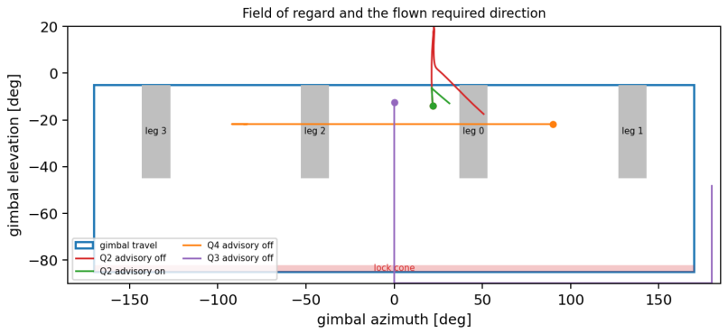
Figure 20.
Q2, accelerating toward a low station, advisory off (red) and on (green): true and predicted margin, tilt, urgency and acceptance, the terminal’s optical error and the received power.
Figure 20.
Q2, accelerating toward a low station, advisory off (red) and on (green): true and predicted margin, tilt, urgency and acceptance, the terminal’s optical error and the received power.
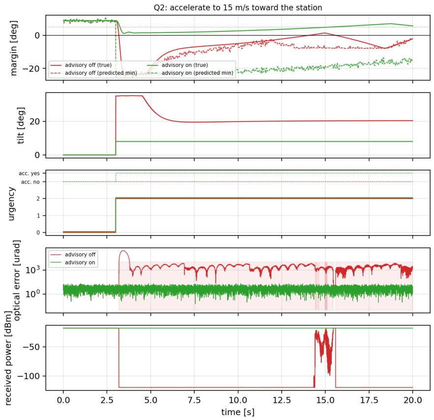
Figure 21.
Quadrotor study: time with the link blocked (left) and optical error while the link is held (right) for every flight Q1–Q7, advisory off against advisory on; medians over the flown seeds.
Figure 21.
Quadrotor study: time with the link blocked (left) and optical error while the link is held (right) for every flight Q1–Q7, advisory off against advisory on; medians over the flown seeds.
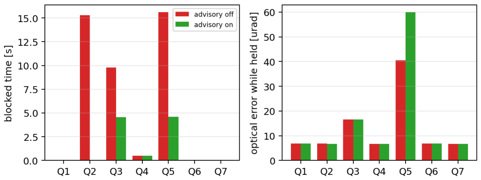
Q1 and Q6, hovering, are clean. The link is never blocked and the terminal holds , the number of Section 3.1; in the / wind with gusts the quadrotor tilts up to and the terminal, in the vibration environment, holds (QT1, QT6 pass). Hovering into a wind is a fixed tilt the geometry absorbs.
Q2 is the quadrotor’s wing crossing, and the tilt limit is its bank limit. Accelerating toward a station below the horizon pitches the nose down by and then by the that / of drag requires, and the required elevation rises into the rotor discs: blocked for 15.3 of on every seed (Figure 20, red). The coordinator sees it at the command and advises the tilt limit; the autopilot accepts at urgency 2, the quadrotor accelerates gently and settles at the speed that of drag allows, 9.1 against / (61 % of the command), and the link is never blocked, at (QT2 passes on both clauses). The cost is speed rather than time, as the predictor of Section 2.15 said it would be.
Q3 and Q5 show what the free yaw is worth—and what it is not. In the overflight the lock cone is predicted ahead and crossed regardless, as it must be; afterwards the station is behind, and where the fixed-wing aircraft stayed blocked, the quadrotor yaws and carries the link on its side: 9.8 to (the Q3 time series of Supplementary Report S3, QT3 passes). In the crossing, the partner starts exactly behind a landing leg and stays there for most of the straight flight; a yaw moves it off the leg, 15.6 to (QT5 passes). The lock fractions in those two rows are the honest part: 56.8 % in the overflight and 0.0 % in the crossing with the advisory on. Both are close-range flights with the partner moving across the line of sight at several centiradians per second, and the terminal’s fixed-gain line-of-sight estimate does not keep the fine stage inside its range—the same limit the fixed-wing overflight and orbit found, here in its strongest form. The advisory fixed the geometry; the terminal’s estimator, not its field of regard, is what loses the link at fifty metres.
Q4, the yaw through the legs, is brief and predicted. Each leg blocks the link for a quarter of a second as the station sweeps past at /, in all, warned ahead (QT4 passes); the coordinator tried the other way round and found it no better, because a yaw passes two legs either way, and said so.
Q7, the orbit with the nose to the centre, is the case the quadrotor does best. Never blocked, lock 100 % and through forty seconds of continuous tilt and / of yaw, against the fixed-wing orbit’s 80.2 %. The difference is consistent with the geometry: with the nose held on the station, the required gimbal direction is nearly constant in the body frame and the body rate carries the motion through the fast channel, whereas the fixed-wing orbit around an off-centre station moved the line of sight in the body frame and left it to the slow channel.
Across the two vehicles. The fixed-wing aircraft loses the link to its wing and its tail and can answer only with a gentler bank; the quadrotor loses it to its rotor discs when it hurries and to its legs when it yaws, and can answer with a gentler tilt and with its heading. What neither can answer is the terminal’s own limit at short range.
3.5. Link Availability and Delivered Data Per Flight
Table 24 restates the flight results in the unit an IoT designer uses; the delivered data is an upper bound on what a real link would carry and an exact statement of what the pointing allows. Three readings follow. Straight flight and orbits deliver what the geometry allows: F1, F5, Q1, Q6 and Q7 are at full availability, and what F6 and F7 lose is lost to lock drops, not to blockage. Where the airframe would block the beam, the advisory is the difference between a lost leg and a full one: the wing crossing F2 goes from 25.3 to 30.0 Gbit and the quadrotor acceleration Q2 from 3.4 to 20.0 Gbit, at the cost of the slower turn and acceleration reported above; over the seven flights of each vehicle the advisory raises the delivered data from 157 to 166 Gbit on the fixed wing and from 123 to 137 Gbit on the quadrotor. Over its sensors, the terminal itself is the limit: the overflights F3 and Q3 and the close crossing Q5 deliver the least, and the advisory changes little there (in Q5 it lowers the availability, because the free yaw it asks for moves the partner off the leg but keeps it moving across the line of sight), for the reason given under F3 in Section 3.3.
4. Discussion
4.1. Limitations of the Control-Law Benchmark
4.1.1. How the Numbers Compare with Reported Terminals
The coarse stage lands where the literature puts coarse stages: published two-stage terminals describe the gimbal as a milliradian-class device handling large, low-frequency excursions, with the fine stage carrying the microradian-class residual [3,9,10,11], and the survey of coarse pointing modules by Dhruv and Kaushal [10] places gimbals of this size and bandwidth in the same class; our coarse residuals are about a milliradian or below across the families that hold lock. The final optical error is the interesting discrepancy. Fast-steering-mirror studies report a few microradians or less on the bench under injected vibration [21,24,26,27,28,29], and a space terminal reports sub-second acquisition with high-accuracy pointing [51], whereas our best full-terminal figure is several times larger. This is not a defect of the model: a bench figure characterises the mirror loop with the beam already on the detector and the reference known, whereas our number is what survives after a navigation solution, an attitude estimate with bias and drift, a coarse loop tracking a moving line of sight and a detector with finite gap and quantisation have each contributed, and the attitude error enters the reference directly, where no fine-stage bandwidth removes it. A terminal-level number cannot be compared with a bench number without saying which contributions are inside it, which is the ambiguity this benchmark exists to remove.
4.1.2. Limitations
A part being real does not make the terminal real: the assembly is a parametric reference, and axis friction and mirror damping remain assumed because no datasheet publishes them and no bench exists to identify them; the uncertainty series draws them at and per cent so that the question a reader needs answered—does the ranking survive not knowing them?—is measured rather than argued. The actuator torque limit is the datasheet peak of a named part chosen by requirement ( , at 36 per cent of peak for the sizing axis), and the ranking is conditional on it. Seed counts are modest (eight paired seeds per cell, twelve on the plant-uncertainty series) and there is no hardware validation. The tuning budget, the search space each family is allowed, the margin screen and the choice of nominal scenarios all shape the ranking; each was fixed before the runs and is discussed, with the alternatives that were tried, in Supplementary Report S1.
4.2. Running the Terminal Side Embedded
The new terminal-side computation is well under ten thousand multiply-adds per (one quaternion-to-direction-cosine conversion, two matrix-vector products and two arctangents, repeated by the monitor and the coordinator). The constraint that is new is on the message side: every advisory carries an expiry, so that a lost message cannot leave the autopilot holding a stale bank limit.
4.3. Limitations of the Flight Study
The terminal simulator keeps its small-angle line-of-sight residual and has no mechanical stop, so a blocked direction is a fade to zero, not a gimbal against its stop; the airframe mask is a set of rectangles, not a measured silhouette; the navigation error seen by the monitor is white and uncorrelated with the terminal’s own; the partner’s navigation radio is a latency parameter; scintillation is not modelled beyond the S1–S8 scenarios; and the aircraft coefficients are a textbook table for an aircraft of the right class.
4.4. What the Three Studies Say Together, and What It Means for an Aerial IoT Backhaul
Read together, the three parts answer one question—what limits the pointing of an optical terminal on a small aircraft—at three time scales, and the answers nest: the fine stage decides the control ranking; the estimators matter only where they touch the loop’s phase at crossover; and at the slowest scale the geometry decides, so the useful thing the terminal can do is to see a crossing coming in the autopilot’s intent and ask for a gentler manoeuvre. For the network designer this collapses into the data a flight delivers (Table 24): at the ranges flown every loss in that table is a pointing loss, a blocked direction or a lost lock, not a link-budget loss; the cheapest gain is the advisory message, at no cost in hardware; and a deployment that collects at short range and relays at long range should expect its losses at the collection end, where the fix is the estimator of Section 3.2, not a larger gimbal. All of it is simulation, on a second plant that is a scaled copy of the first and against textbook autopilots; the next validation steps are those of Section 5.
5. Conclusions
One simulation benchmark, checked step by step, tested four sets of statements written down before the runs (Table 14, Table 17, Table 21 and Table 23); each is answered here with its number.
Control laws (P1–P4: all four hold). The coarse residuals of the families that hold lock stay within a factor of 1.6 (P1), the two-stage rejection spreads them by a factor of 70 (P2), the rank correlation between rejection and optical error is -1.00 (P3) and the ranking is the same on both plants (P4). Answer to the first question: run the disturbance-observer family C6, because the fine stage decides the ranking.
Estimators (H1–H6: three hold, three fail). H1 fails: a rate filter that does not know the torque does not stay within 10 per cent of C6’s error but loses lock. H2 fails: no candidate halves the failure probability on the sensor-degradation scenario. H3 fails: no fine-stage candidate improves the error by more than 10 per cent. H4 holds: the line-of-sight candidates change it by less than 5 per cent. H5 holds: Q31 storage changes it by less than 2 per cent. H6 holds: one tick of latency costs more than 20 per cent. Answer to the second question: at the gimbal rate, a Kalman filter that knows the applied torque; everywhere else the present simple filters; never a filter that adds a tick.
Fixed-wing flights (T1–T7: four hold, three fail). T1, T3, T5 and T7 hold. T2 fails on its cost clause: the link is kept on every seed, but the turn takes +65 % longer, not less than 10. T4 fails on its last clause: the flight plan wins as designed, but the autopilot accepted advisories during the turn instead of none. T6 fails on its error clause: the link is kept, but the held error exceeds the reference by more than the 20 per cent allowed.
Quadrotor flights (QT1–QT7: all seven hold). The tilt limit keeps the link through the acceleration at 61 per cent of the commanded speed (QT2); the free-yaw advisory at least halves the blocked time in the overflight and the crossing (QT3, QT5); the legs block briefly and with warning (QT4); the wind flight and the orbit are never blocked (QT6, QT7). Answer to the third question: the link survives the aircraft’s own manoeuvres when the terminal sees them in the autopilot’s intent a few seconds ahead and the autopilot accepts a gentler bank or tilt, another turn direction or a free heading; it does not survive where the flight plan itself puts the station behind the airframe, and at short range it is lost by the terminal’s own line-of-sight estimate. The three failed clauses and the short-range result point at the next steps: a hardware step response of the gimbal, a line-of-sight estimator for short range, and a released autopilot in the loop.
Supplementary Materials
The following supporting information can be downloaded at the website of this paper posted on Preprints.org.
Appendix A. Design Models, Shared Conditioning, and the Sources and Search Spaces of Every Law and Filter
Appendix A.1. What Is Ours and What Is Used as Published
The six control families and the seven filter variants are standard methods, used as their sources publish them; their derivations are not repeated here. What this appendix gives is the part that is specific to this study and that a reader needs to reproduce the runs: the design models each law was synthesised on, the signal conditioning every family shares, and, for each family and each filter, the source, the parameters the search varied and the one implementation choice that is not obvious from the source. Every equation is the one the released code executes. Symbols: J and B are the axis inertia and viscous friction, the motor torque, the encoder angle, the mirror angle, T the controller period ( coarse, fine), and angular frequency in .
Appendix A.1.1. Design Models
Every synthesis is carried out on the linear one-axis design model, and the resulting controller is then evaluated on the full nonlinear terminal. For a coarse axis the model is the rigid body with viscous friction,
with J and B per axis from the CAD-derived plant. Coulomb friction, the elevation gravity torque , the inertia coupling between axes, the current loop and the structural mode are all absent from the design model and present in the evaluation plant.
For the fine stage the model is the mirror’s second-order response to its angle command u,
with , and . The fine loop does not measure . It measures the optical error the quadrant detector reports, referred to the mirror by the optical gain, , where d is the coarse residual referred to the mirror. Its reference is therefore zero and d is an outside signal the loop must reject. Three families (C1’s analytic rule, C2 and C3) are designed against (A2) in full; C4, C5 and C6 are designed against the double-integrator form of the same mirror, obtained by treating (A2) as with
so that has the same input gain and damping as the mirror and no stiffness. This mapping is the one choice here that is not in the sources. Handing these families the mirror’s DC gain instead of is the tempting error: it scales their command by and parks the mirror on its stop from the first tick.
Appendix A.1.2. Shared Conditioning
The following are identical for every family and sit outside the control law. The measured rate is a filtered backward difference of the quantised encoder,
with and . The reference rate is the commanded tracking rate passed through a first-order filter at , and the acceleration feed-forward is passed through the same filter; every family receives additively with unit gain. Every command is clipped to the actuator limit, for the motor and for the mirror, in one shared function. Every integrator uses one anti-windup rule: it is frozen when the output is saturated and the error has the sign that would drive it further into saturation. Every estimator is initialised from the first measurement and the tracking rate, and re-initialised from the current measurement at each mode transition (Section 2.3.4).
Appendix A.1.3. The Control Families: Source, Search Space and the One Non-Obvious Choice
Table A1 lists, for each family, the source whose form is implemented, the design model it was synthesised on, the parameters the 48-evaluation search varied (Table 4 gives the budget and outcome) and the single implementation choice a reader could not guess from the source; the budget and the feasibility screen are those of Section 2.3.4.
Table A1.
The six control families as implemented: the published form each follows, the design model it was synthesised on, the parameters the equal-budget search varied on both stages unless stated, and the one implementation choice that is specific to this study.
Table A1.
The six control families as implemented: the published form each follows, the design model it was synthesised on, the parameters the equal-budget search varied on both stages unless stated, and the one implementation choice that is specific to this study.
| Family | Published form | Design model | Searched | Choice specific to this study |
|---|---|---|---|---|
| C1 PID | cascaded position/rate PI loops [52,53] | (A1), (A2) | , ; fine | gains computed from J, B so the rate loop is a damped second-order system at and the position loop times slower |
| C2 LQG | Kalman filter plus LQR with an integral state [53,54] | (A1), (A2), zero-order hold | Bryson allowances , , ; covariances , V | every weight declared as a largest acceptable error, accumulated error or torque, so that each has a physical unit |
| C | sampled-data mixed sensitivity, central controller [40,55,56] | (A1), (A2) | , , , (closed form from the weights; not searched) | executed as a state-space recursion; the fine loop is designed against the full mirror model and its result is unstable, as reported in Section 3.1 |
| C4 SMC | boundary-layer sliding mode [57,58] | double integrator (A3) | , K, , | an integral term inside the sliding variable s removes the constant-load sag |
| C5 ADRC | linear ADRC with a third-order extended state observer [41,59] | double integrator with of (A3) | , | the observer is discretised in predictor-corrector form [60]; the held-measurement form carries a rate-proportional bias |
| C6 DOB | PD servo plus disturbance observer [61,62,63] | nominal from (A1) or (A3) | coarse , , ; fine , | realised as one proper second-order state-space filter with corner , so no differentiation of the measurement |
| C7 hybrid | mode switch | – | none | C2 acquires and C6 tracks (Section 2.3.4) |
Appendix A.1.4. The Filter Variants: Source and Form
Table A2 does the same for the estimator candidates of Section 3.2. Two observations from implementing them are worth one sentence each. The -- tracker is the extended state observer of C5 with its poles placed by the tracking index instead of an observer bandwidth: the two literatures describe the same recursion. And the disturbance-augmented filter inherits the discretisation finding of C5 word for word: it must be run in predictor-corrector form.
Table A2.
The seven filter variants as implemented, with the code name the result tables use, the states carried, the known input fed to the prediction, how the gain is set and the published form followed.
Table A2.
The seven filter variants as implemented, with the code name the result tables use, the states carried, the known input fed to the prediction, how the gain is set and the published form followed.
| Variant | Code | States | Known input | Gain | Source |
|---|---|---|---|---|---|
| V1 time-varying Kalman | tvkf | , , covariance P | torque | Riccati recursion every tick, Joseph-form covariance update | [54,64] |
| V2 steady-state Kalman | kf | , | none | fixed, from the discrete Riccati equation | [54] |
| V- / -- | ab, abg | , (, acceleration) | none | closed form from the tracking index | [65] |
| V4 Kalman with torque input | kfu | , | torque | fixed, from the discrete Riccati equation | [54] |
| V5 Kalman on the line of sight | kf at E2 | LOS ℓ, rate | navigation LOS rate | fixed, from a stated LOS-rate random walk and measurement variance | [54] |
| V6 disturbance-augmented | kfd | , , d | torque | fixed, from the discrete Riccati equation | [60] |
| V7 complementary (attitude) | cf | yaw, pitch | gyro rates at 1 | first-order pull toward the AHRS at 2 | [66] |
Appendix B. The Gimbal-Command Geometry the Coupling Uses, and Two Details of the Coupling
Appendix B.1. The Gimbal-Command Geometry the Coupling Uses
These are the formulas behind Section 2.8, in the order a program computes them. They are standard rigid-body geometry, collected here because the coupling of Appendix B.2 and the lock-cone prediction of the monitor depend on their exact form. The autopilot gives the attitude as a unit quaternion, from which the direction-cosine matrix (navigation to body) follows by the usual products of quaternion components; no sine or cosine is evaluated at run time.
The line of sight in the gimbal frame is the difference of the two positions rotated twice,
where is the fixed rotation of the gimbal base on the airframe (the identity for a nose or belly mount aligned with the body axes). With components (forward, right, down) the gimbal command is
the minus sign because z points down and elevation counts up.
How fast the command moves. Differentiating (A5) gives
the first term from the two platforms moving, the second from the body turning under a fixed line of sight ( is the body rate from the gyro); the azimuth and elevation rates follow by the chain rule of (A6), and the azimuth rate is unbounded where : that is the lock cone.
The rotation part alone, which the terminal’s feedforward needs, is in closed form, with , and body rates ,
In words: yawing at rate r turns the required azimuth at ; rolling at p or pitching at q moves the required elevation by the part of that rate that lies across the line of sight, and also moves the azimuth by an amount that grows with : small near the horizon, large when the gimbal looks steeply down.
The embedding into the terminal. The terminal of the earlier parts of this article commands “line of sight minus yaw and pitch”. The coupling therefore hands it , (eq. (4) in the body), so that its own subtraction returns the exact .
Appendix B.2. Two Details of the Coupling
Both were found by tracing the terminal through a banked turn, after the first version of the coupling lost lock on every roll-in.
The terminal’s feedforward is exact only near the horizon. The terminal simulator projects the body rate onto the gimbal axes with for azimuth, which omits the term of (A8); at the elevation of the flights here the omission is a third of the roll rate. Rather than change the terminal simulator’s code (and break the bit-for-bit chain between the studies), the co-simulation hands the terminal the equivalent body rates for which its own projection gives (A8): from the azimuth equation, and the smallest change of that satisfies the elevation equation. The test suite checks the identity to . A terminal firmware would simply use (A8).
The roll must arrive through the fast channel. The terminal holds its line-of-sight estimate at and takes the platform motion through its attitude at . If the roll effect is put into the line of sight, the position reference goes stale by up to between updates and lock is lost on every roll-in, whatever the roll rate. The coupling therefore hands the terminal the true inertial line of sight (slow) and an effective yaw and pitch, the line of sight minus the exact gimbal angles, which carries the roll effect at the fast rate. With both details in place the terminal holds through the banked roll-in of the wing crossing.
References
- Kaushal, H.; Kaddoum, G. Optical Communication in Space: Challenges and Mitigation Techniques. IEEE Communications Surveys & Tutorials, 2017. [Google Scholar]
- Khalighi, M.A.; Uysal, M. Survey on Free Space Optical Communication: A Communication Theory Perspective. IEEE Communications Surveys & Tutorials, 2014. [Google Scholar]
- Kaymak, Y.; Rojas-Cessa, R.; Feng, J.; Ansari, N.; Zhou, M.; Zhang, T. A Survey on Acquisition, Tracking, and Pointing Mechanisms for Mobile Free-Space Optical Communications. IEEE Communications Surveys & Tutorials, 2018. [Google Scholar]
- Alimi, I.A.; Monteiro, P.P. Revolutionizing Free-Space Optics: A Survey of Enabling Technologies, Challenges, Trends, and Prospects of Beyond 5G Free-Space Optical (FSO) Communication Systems. Sensors 2024, 24, 8036. [Google Scholar] [CrossRef]
- Phuchortham, S.; Sabit, H. A Survey on Free-Space Optical Communication with RF Backup: Models, Simulations, Experience, Machine Learning, Challenges and Future Directions. Sensors 2025, 25, 3310. [Google Scholar] [CrossRef]
- Singh, D.; R, S. Comprehensive Performance Analysis of Hovering UAV-Based FSO Communication System. IEEE Photonics J. 2022, 14, 1–13. [Google Scholar] [CrossRef]
- Bashir, M.S.; Alouini, M.S. Optimal Positioning of Hovering UAV Relays for Mitigation of Pointing Error in Free-Space Optical Communications. IEEE Trans. Commun. 2022, 70, 7477–7490. [Google Scholar] [CrossRef]
- Kang, J. Joint Divergence Angle of Free Space Optics (FSO) Link and UAV Trajectory Design in FSO-Based UAV-Enabled Wireless Power Transfer Relay Systems. Photonics 2024, 11, 1136. [Google Scholar] [CrossRef]
- Abdelfatah, R.; Alshaer, N.; Ismail, T. A Review on Pointing, Acquisition, and Tracking Approaches in UAV-Based FSO Communication Systems. Opt. Quantum Electron. 2022, 54, 571. [Google Scholar] [CrossRef]
- Dhruv; Kaushal, H. A Review of Pointing Modules and Gimbal Systems for Free-Space Optical Communication in Non-Terrestrial Platforms. Photonics 2025, 12, 1001. [Google Scholar] [CrossRef]
- Duliu, A.; Shrestha, A. Software Architecture for Multi-Domain Pointing, Acquisition and Tracking in Free-Space Optical Communication. In Proceedings of the 2025 IEEE International Conference on Space Optical Systems and Applications (ICSOS); IEEE, 2025; pp. 1–4. [Google Scholar] [CrossRef]
- Chen, L.; Zhu, L.; Du, H.; Wang, X.; Shen, S.; Wang, Y.; Zhao, S.; Wang, X. Pointing Acquisition and Tracking System for Free Space Optical Communication Based on Integrated Optical Phased Array. IEEE Photonics J. 2025, 17, 1–8. [Google Scholar] [CrossRef]
- Chung, Y.H.; Lee, D.; Lee, H.; Oh, S. Enhanced 2-axis Gimbal Stabilization Control via a Hybrid Coordinate System Approach With Disturbance Observer. Int. J. Control Autom. Syst. 2025, 23, 3248–3256. [Google Scholar] [CrossRef]
- Deng, J.; Duan, Q.; Mao, Y.; Bao, Q. Stability Margins of Disturbance Observer: Addressing Uncertainty and Time Delay in Line-of-Sight Stabilization Systems. In Proceedings of the IECON 2025 – 51st Annual Conference of the IEEE Industrial Electronics Society; IEEE, 2025; pp. 1–8. [Google Scholar] [CrossRef]
- Chang, S.; Yang, D.; Cao, J.; Li, X. An Extend Sliding Mode Disturbance Observer for Optical Inertial Platform Line-of–Sight Stabilized Control. Machines 2024, 12, 849. [Google Scholar] [CrossRef]
- Ma, R.; Wang, Q.; Li, J.; Xia, Y.; Yuan, L.; Yuan, J.; Shi, J.; Liu, X.; Tu, Q.; Tang, T.; et al. Robust Risley prism control based on disturbance observer for system line-of-sight stabilization. Appl. Opt. 2022, 61, 3463. [Google Scholar] [CrossRef]
- Yang, Y.; Cui, Y.; Qiao, J.; Zhu, Y. Adaptive periodic-disturbance observer based composite control for SGCMG gimbal servo system with rotor vibration. Control Eng. Pract. 2023, 132, 105407. [Google Scholar] [CrossRef]
- Zhang, L.; Guo, X.; Yao, X.; Cui, Y. Adaptive Fixed-Time Refined Disturbance Observer-Based Composite Control for Gimbal Servo System With Multiple Disturbances. IEEE/ASME Trans. Mechatron. 2026, 1–12. [Google Scholar] [CrossRef]
- Bian, Q.; Miao, Q.; Feng, N.; Li, X.; Tang, T. High-Bandwidth Acceleration Disturbance Observer Control With Nonlinear Function for Inertially Stabilized Gimbal of Moving Platform. IEEE Trans. Autom. Sci. Eng. 2026, 23, 968–978. [Google Scholar] [CrossRef]
- Wang, Z.; Wang, Y.; Xu, R.; Tong, J.; Tian, D. Fast disturbance rejection for inertial stabilization platforms based on a nonlinear adaptive sliding-mode-assisted disturbance observer. ISA Trans. 2026, 177, 819–828. [Google Scholar] [CrossRef]
- Li, Z.; Li, L.; Zhang, J.; Feng, W. System modeling and sliding mode control of fast steering mirror for space laser communication. Mech. Syst. Signal Process. 2024, 211, 111206. [Google Scholar] [CrossRef]
- Kim, J.G. System Integration Design of High-Performance Piezo-Actuated Fast-Steering Mirror for Laser Beam Steering System. Sensors 2024, 24, 6775. [Google Scholar] [CrossRef]
- Zhong, J.; Nishida, R.; Shinshi, T. Design and precision tracking control of a high-bandwidth fast steering mirror for laser beam machining. Precis. Eng. 2022, 73, 128–139. [Google Scholar] [CrossRef]
- Pechgraber, D.; Csencsics, E.; Schitter, G. High-precision pointing control with optimization-based parameter tuning for switched amplifier-driven 2D fast steering mirror in optical laser communication. Precis. Eng. 2026, 102, 138–147. [Google Scholar] [CrossRef]
- Chen, Y.; Zhu, F.; Huang, R.; Chen, Q.; Wang, J.; Feng, J.; Yang, S. Two-level piezo actuated fast steering mirror with large deflection range and low tracking error for intersatellite laser beam pointing control. Results Eng. 2026, 32, 111716. [Google Scholar] [CrossRef]
- Wang, L.; Zhang, F.; Sun, H.; Zhao, J.; He, Y.; Zan, R.; Gao, P.; Wang, C. High-Dynamic Tracking Control Technology for the Fast-Steering Mirror in a Laser Communication System. Appl. Opt. 2025, 64, 8240–8247. [Google Scholar] [CrossRef]
- Yang, S.; Li, X.; Li, Y. Design of an MPC with hysteresis compensation for high-accuracy trajectory tracking of piezoelectric fast steering mirrors. Control Eng. Pract. 2026, 169, 106766. [Google Scholar] [CrossRef]
- Chen, Y.; Zhu, F.; Huang, R.; Chen, Q.; Wang, J.; Feng, J.; Yang, S. Two-level piezo actuated fast steering mirror with large deflection range and low tracking error for intersatellite laser beam pointing control. Results Eng. 2026, 32, 111716. [Google Scholar] [CrossRef]
- Jia, X.; Chen, Q.; Liu, L.; Xia, R. A Double-Integral Global Fast Terminal Sliding Mode Control with TD-LESO for Chattering Suppression and Precision Tracking of Fast Steering Mirrors. Actuators 2026, 15, 46. [Google Scholar] [CrossRef]
- Koubâa, A.; Allouch, A.; Alajlan, M.; Javed, Y.; Belghith, A.; Khalgui, M. Micro Air Vehicle Link (MAVLink) in a nutshell: a survey. IEEE Access 2019, 7, 87658–87680. [Google Scholar] [CrossRef]
- Aliane, N. A Survey of Pixhawk/PX4 Autopilot and Its Impact on Research and Education. Comput. Mater. Contin. 2026, 87, 1–10. [Google Scholar] [CrossRef]
- Bopalkar, A.; Patil, D.; Somvanshi, H. Offboard Control of Autonomous Drones in Ros2-Px4 Simulated Environments. In Proceedings of the 2025 IEEE 4th World Conference on Applied Intelligence and Computing (AIC); IEEE, 2025; pp. 763–768. [Google Scholar] [CrossRef]
- Rüddenklau, R.; Barone, S.; Garbagnati, E.; Spier, S.; Schitter, G. Feed-Forward Compensation of Body-Pointing Uncertainties for Laser Communication Terminals. J. Guid. Control Dyn. 2026, 49, 1810–1819. [Google Scholar] [CrossRef]
- Haider, S.A.; Ahmad, K.M.; Khan, A.A. Efficient unmanned aerial vehicle-based data collection for IoT smart farming. Internet Things 2024, 26, 101184. [Google Scholar] [CrossRef]
- Sabzehali, J.; Shah, V.K.; Fan, Q.; Choudhury, B.; Liu, L.; Reed, J.H. Optimizing Number, Placement, and Backhaul Connectivity of Multi-UAV Networks. IEEE Internet Things J. 2022, 9, 21548–21560. [Google Scholar] [CrossRef]
- Chen, R.; Wang, W.; Wu, W. An Adjustable Wireless Backhaul Link Selection Algorithm for LEO-UAV-Sensor-Based Internet of Remote Things Network. Sensors 2024, 24, 1973. [Google Scholar] [CrossRef]
- Panahi, F.H.; Panahi, F.H.; Nourmohammadi, F. Intelligent UAV-Assisted Optical Wireless Networks for Sustainable Internet of Underwater Things. IEEE Internet Things J. 2026, 1–1. [Google Scholar] [CrossRef]
- Li, B.; Liu, J.; Liang, Y.; Li, Q.; Liu, H.; Zhang, Y.; Mu, J.; Mumtaz, S.; Chen, S. UAV-Enabled Joint Sensing, Communication, Powering, and Backhaul Transmission in Maritime Monitoring Networks. IEEE Internet Things J. 2026, 13, 7473–7486. [Google Scholar] [CrossRef]
- Sliti, M.; Ghafoor, S.; Ayouni, S.; Mrabet, M.; Ammar, L.B.; Ijaz, M. Line-of-sight stability in unmanned aerial vehicle relays for hybrid free-space optical and visible light communication links under atmospheric effects. PLoS ONE 2026, 21, e0343564. [Google Scholar] [CrossRef]
- Doyle, J.C.; Glover, K.; Khargonekar, P.P.; Francis, B.A. State-Space Solutions to Standard H2 and H∞ Control Problems. IEEE Transactions on Automatic Control, 1989. [Google Scholar]
- Gao, Z. Scaling and Bandwidth-Parameterization Based Controller Tuning. In Proceedings of the Proc. American Control Conference, 2003. [Google Scholar]
- Bierman, G.J. Factorization Methods for Discrete Sequential Estimation; Academic Press, 1977. [Google Scholar]
- Stevens, B.L.; Lewis, F.L.; Johnson, E.N. Aircraft Control and Simulation: Dynamics, Controls Design, and Autonomous Systems, 3rd ed.; Wiley: Hoboken, NJ, 2015. [Google Scholar]
- Beard, R.W.; McLain, T.W. Small Unmanned Aircraft: Theory and Practice; Princeton University Press: Princeton, NJ, 2012. [Google Scholar]
- Andrews, L.C.; Phillips, R.L.; Hopen, C.Y. Laser Beam Scintillation with Applications; SPIE Press: Bellingham, WA, 2001. [Google Scholar]
- Efron, B. Bootstrap Methods: Another Look at the Jackknife. Ann. Stat. 1979. [Google Scholar] [CrossRef]
- Friedman, M. The Use of Ranks to Avoid the Assumption of Normality Implicit in the Analysis of Variance. J. Am. Stat. Assoc. 1937. [Google Scholar] [CrossRef]
- Wilcoxon, F. Individual Comparisons by Ranking Methods. Biom. Bull. 1945. [Google Scholar] [CrossRef]
- Holm, S. A Simple Sequentially Rejective Multiple Test Procedure. Scand. J. Stat. 1979. [Google Scholar]
- Freefly Systems. ALTA X specifications empty weight 10.86 kg, maximum take-off 34.86 kg, maximum payload 15.06 kg, unfolded diameter 1415 mm, 33x9 in propellers, 44.4 V, 115 rpm/V; thrust ratio 2.5:1 from the product page. 2026. Available online: https://freeflysystems.com/alta-x/specs (accessed on 2026-09-22).
- Wang, J.; Su, Z.; Li, B.; Zheng, W.; Gao, H. High-accuracy pointing and sub-second acquisition in a space optical communication terminal with ground-based verification method. Opt. Laser Technol. 2026, 193, 114313. [Google Scholar] [CrossRef]
- Åström, K.J.; Hägglund, T. Advanced PID Control; ISA, 2006. [Google Scholar]
- Franklin, G.F.; Powell, J.D.; Workman, M. Digital Control of Dynamic Systems, 3rd ed.; Addison-Wesley, 1998. [Google Scholar]
- Simon, D. Optimal State Estimation: Kalman, H∞, and Nonlinear Approaches; Wiley, 2006. [Google Scholar]
- Zhou, K.; Doyle, J.C.; Glover, K. Robust and Optimal Control; Prentice Hall, 1996. [Google Scholar]
- Skogestad, S.; Postlethwaite, I. Multivariable Feedback Control: Analysis and Design, 2nd ed.; Wiley, 2005. [Google Scholar]
- Utkin, V.I. Variable Structure Systems with Sliding Modes. IEEE Transactions on Automatic Control, 1977. [Google Scholar]
- Shtessel, Y.; Edwards, C.; Fridman, L.; Levant, A. Sliding Mode Control and Observation; Birkhäuser: Basel, 2014. [Google Scholar] [CrossRef]
- Herbst, G. A Simulative Study on Active Disturbance Rejection Control (ADRC) as a Control Tool for Practitioners. Electronics 2013, 2, 246–279. [Google Scholar] [CrossRef]
- Miklosovic, R.; Radke, A.; Gao, Z. Discrete implementation and generalization of the extended state observer. In Proceedings of the Proc. American Control Conference, 2006; pp. 2209–2214. [Google Scholar] [CrossRef]
- Ohnishi, K.; Shibata, M.; Murakami, T. Motion Control for Advanced Mechatronics. IEEE/ASME Transactions on Mechatronics, 1996. [Google Scholar]
- Umeno, T.; Hori, Y. Robust Speed Control of DC Servomotors Using Modern Two Degrees-of-Freedom Controller Design. IEEE Transactions on Industrial Electronics, 1991. [Google Scholar]
- Sariyildiz, E.; Oboe, R.; Ohnishi, K. Disturbance Observer-Based Robust Control and Its Applications: 35th Anniversary Overview. IEEE Trans. Ind. Electron. 2020, 67, 2042–2053. [Google Scholar] [CrossRef]
- Kalman, R.E. A New Approach to Linear Filtering and Prediction Problems. J. Basic Eng. 1960. [Google Scholar] [CrossRef]
- Kalata, P.R. The Tracking Index: A Generalized Parameter for α-β and α-β-γ Target Trackers. IEEE Trans. Aerosp. Electron. Syst. 1984, AES-20, 174–182. [Google Scholar] [CrossRef]
- Mahony, R.; Hamel, T.; Pflimlin, J.M. Nonlinear Complementary Filters on the Special Orthogonal Group. IEEE Trans. Autom. Control 2008, 53, 1203–1218. [Google Scholar] [CrossRef]
Figure 1.
Component breakdown of the reference assembly. (a) Every solid, with its principal dimensions in millimetres. (b) Side elevation with the payload housing drawn as an outline, so the relay tube and FSM mount it contains are visible. Group membership is not cosmetic: the azimuth inertia carries everything above the base and the elevation inertia everything above the elevation axis, so a misassignment propagates directly into and . The payload centre of mass lies 30 above the elevation axis; a production terminal would balance that out, and it is kept here because it makes the unmodelled gravity torque explicit.
Figure 1.
Component breakdown of the reference assembly. (a) Every solid, with its principal dimensions in millimetres. (b) Side elevation with the payload housing drawn as an outline, so the relay tube and FSM mount it contains are visible. Group membership is not cosmetic: the azimuth inertia carries everything above the base and the elevation inertia everything above the elevation axis, so a misassignment propagates directly into and . The payload centre of mass lies 30 above the elevation axis; a production terminal would balance that out, and it is kept here because it makes the unmodelled gravity torque explicit.
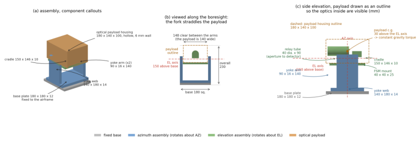
Figure 2.
Where the parameters of Table 1 and Table 2 live. (a) The coarse stage: elevation inertia depends on orientation and the unbalanced payload applies a constant gravity torque, which is absent from every controller’s design model and must be absorbed by integral action. (b) The receiver train; the beam-split ratio divides power between the data and tracking branches and is swept as a design variable. (c) Detector geometry: the quadrant sums are integrated in closed form over each rectangle. (d) The error sources that bound what any controller can achieve, and which therefore set the floor the comparison is measured against.
Figure 2.
Where the parameters of Table 1 and Table 2 live. (a) The coarse stage: elevation inertia depends on orientation and the unbalanced payload applies a constant gravity torque, which is absent from every controller’s design model and must be absorbed by integral action. (b) The receiver train; the beam-split ratio divides power between the data and tracking branches and is swept as a design variable. (c) Detector geometry: the quadrant sums are integrated in closed form over each rectangle. (d) The error sources that bound what any controller can achieve, and which therefore set the floor the comparison is measured against.
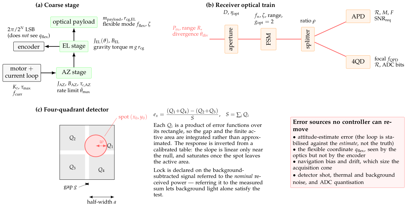
Figure 3.
The two control loops. Every controller family occupies only the two shaded boxes: reference conditioning, feed-forward filtering, saturation limits, the anti-windup rule and every measurement are identical across families, so a difference in the results is a difference between control laws rather than between implementations. The coarse loop is inertially stabilised against the attitude estimate rather than the truth, so attitude error appears as a pointing error no controller can remove, and the encoder does not observe the flexible coordinate that the optics see. The fine loop regulates the measured optical error to zero rather than tracking a mirror-angle reference, and slowly hands its mean deflection back to the coarse stage (recentering) so that mirror range is reserved for the high-frequency residual.
Figure 3.
The two control loops. Every controller family occupies only the two shaded boxes: reference conditioning, feed-forward filtering, saturation limits, the anti-windup rule and every measurement are identical across families, so a difference in the results is a difference between control laws rather than between implementations. The coarse loop is inertially stabilised against the attitude estimate rather than the truth, so attitude error appears as a pointing error no controller can remove, and the encoder does not observe the flexible coordinate that the optics see. The fine loop regulates the measured optical error to zero rather than tracking a mirror-angle reference, and slowly hands its mean deflection back to the coarse stage (recentering) so that mirror range is reserved for the high-frequency residual.
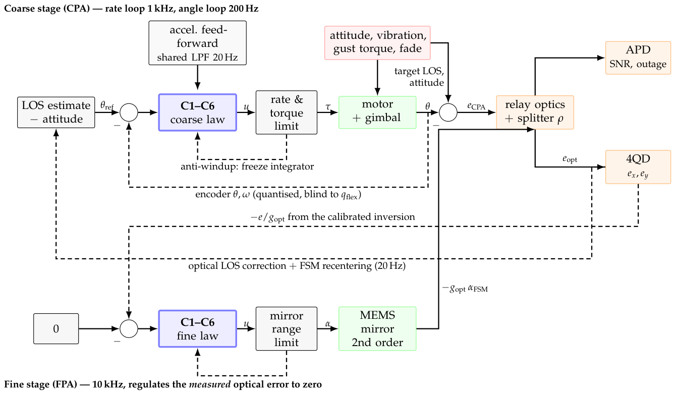
Figure 4.
Thefour estimation points. E1 turns a quantised encoder into a rate; E2 fuses the optical error and the navigation solution into a line-of-sight estimate; E3 is the attitude estimate the coarse loop stabilises against; E4 turns the detector’s error into the position, rate and (for some laws) disturbance the fine law uses. The control-law benchmark (Section 3.1) runs a fixed simple filter at each.
Figure 4.
Thefour estimation points. E1 turns a quantised encoder into a rate; E2 fuses the optical error and the navigation solution into a line-of-sight estimate; E3 is the attitude estimate the coarse loop stabilises against; E4 turns the detector’s error into the position, rate and (for some laws) disturbance the fine law uses. The control-law benchmark (Section 3.1) runs a fixed simple filter at each.
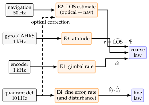
Figure 5.
The co-simulation. Blue: new models (flight, navigation, link partner, channel). Orange: the terminal side, of which the simulator is the code of the control-law benchmark (Section 3.1) unchanged and the geometry and monitor blocks are new. Green: the autopilot. Solid arrows are data that already flow in the earlier benchmarks (Section 3.1 and Section 3.2) or are their natural extension; the dashed red arrow is the one new direction, the advisory from the terminal to the autopilot. The monitor uses the same navigation and partner inputs as the geometry block.
Figure 5.
The co-simulation. Blue: new models (flight, navigation, link partner, channel). Orange: the terminal side, of which the simulator is the code of the control-law benchmark (Section 3.1) unchanged and the geometry and monitor blocks are new. Green: the autopilot. Solid arrows are data that already flow in the earlier benchmarks (Section 3.1 and Section 3.2) or are their natural extension; the dashed red arrow is the one new direction, the advisory from the terminal to the autopilot. The monitor uses the same navigation and partner inputs as the geometry block.
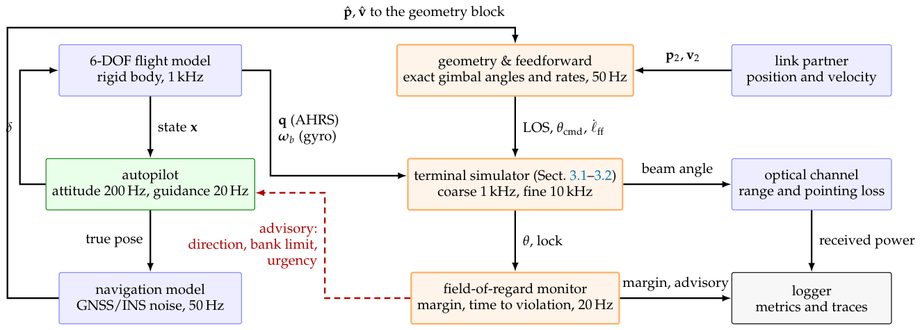
Figure 6.
The chain of frames. The link partner’s position relative to the aircraft is rotated by the attitude into the body frame and by the fixed mounting rotation into the gimbal base frame; the azimuth and elevation of that vector are the gimbal command. The formulas are in Appendix B.1.
Figure 6.
The chain of frames. The link partner’s position relative to the aircraft is rotated by the attitude into the body frame and by the fixed mounting rotation into the gimbal base frame; the azimuth and elevation of that vector are the gimbal command. The formulas are in Appendix B.1.
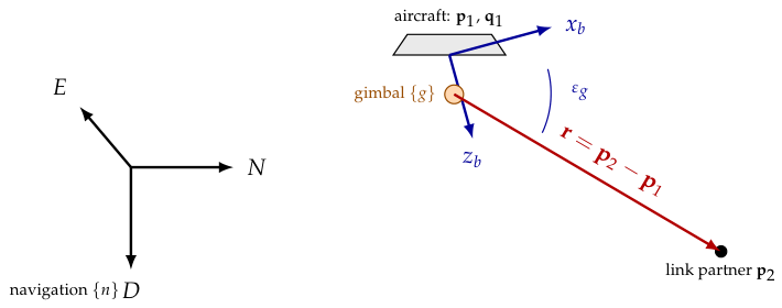
Figure 7.
The coordination state machine on the terminal side, as implemented. Transitions down are on the margin and the time to violation; transitions up carry a hysteresis h (degrees) and (seconds) so that the advisory does not chatter. In WARN, URGENT and BLOCKED the coordinator evaluates its alternatives; the autopilot receives the advisory and decides.
Figure 7.
The coordination state machine on the terminal side, as implemented. Transitions down are on the margin and the time to violation; transitions up carry a hysteresis h (degrees) and (seconds) so that the advisory does not chatter. In WARN, URGENT and BLOCKED the coordinator evaluates its alternatives; the autopilot receives the advisory and decides.
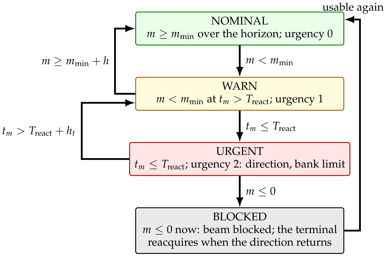
Figure 8.
Coarse residual against final optical error, one point per family on the nominal series, with lines of constant two-stage rejection. Position along a diagonal is the final error; distance below it is how much of the pointing the fine stage is doing. The coarse residuals cluster tightly while the distances below the diagonal differ by well over an order of magnitude, so it is the fine stage and not the gimbal that orders the families.
Figure 8.
Coarse residual against final optical error, one point per family on the nominal series, with lines of constant two-stage rejection. Position along a diagonal is the final error; distance below it is how much of the pointing the fine stage is doing. The coarse residuals cluster tightly while the distances below the diagonal differ by well over an order of magnitude, so it is the fine stage and not the gimbal that orders the families.
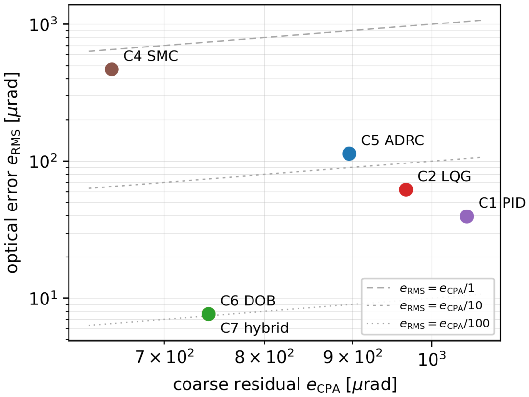
Figure 11.
Transient response to a 2 step, measured on the coarse pointing error. (a) Tracking mode, where the command is a rate limited in acceleration. (b) The same responses inside the band. (c) The pointing-mode command interface: a position command slewed at a fixed rate. (d) Rise time, overshoot and settling time; a missing bar means the response never reached that threshold. The early excursion below zero is the acceleration limit: the error grows before it shrinks, because the commanded rate cannot change instantly.
Figure 11.
Transient response to a 2 step, measured on the coarse pointing error. (a) Tracking mode, where the command is a rate limited in acceleration. (b) The same responses inside the band. (c) The pointing-mode command interface: a position command slewed at a fixed rate. (d) Rise time, overshoot and settling time; a missing bar means the response never reached that threshold. The early excursion below zero is the acceleration limit: the error grows before it shrinks, because the commanded rate cannot change instantly.
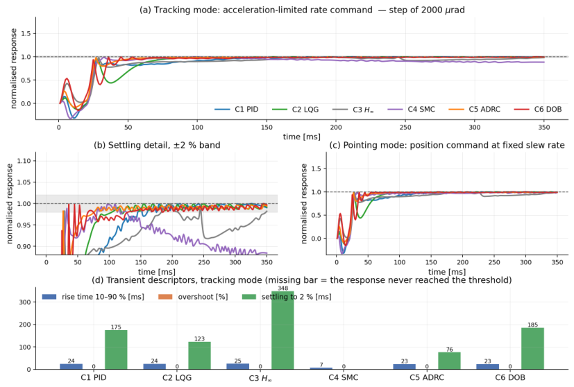
Figure 12.
Coarse-stage open-loop transfer , measured through each family’s own executed controller kernel. Filled circles mark unity crossover; the dotted vertical line is the structural-mode frequency and the dashed line is the controller-rate Nyquist frequency. C6 carries the least phase margin on this stage, about , with the largest sensitivity peak. C3’s magnitude is flat at low frequency where every other family’s rises—the finite DC loop gain that Section 3.1.4 traces to the formulation rather than to the tuning.
Figure 12.
Coarse-stage open-loop transfer , measured through each family’s own executed controller kernel. Filled circles mark unity crossover; the dotted vertical line is the structural-mode frequency and the dashed line is the controller-rate Nyquist frequency. C6 carries the least phase margin on this stage, about , with the largest sensitivity peak. C3’s magnitude is flat at low frequency where every other family’s rises—the finite DC loop gain that Section 3.1.4 traces to the formulation rather than to the tuning.
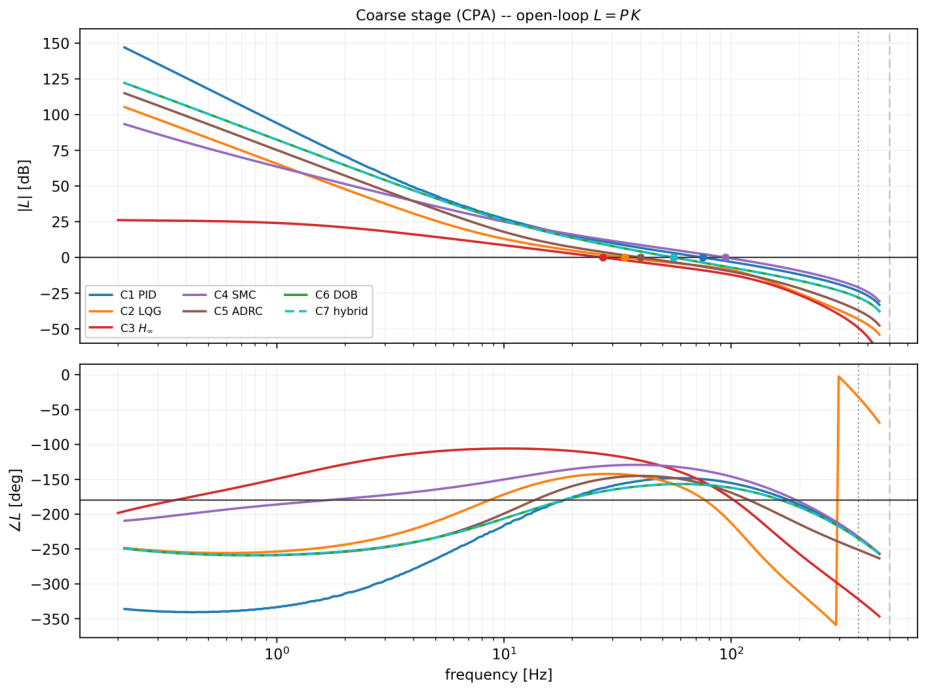
Figure 13.
Frequency response of each rate estimator relative to the ideal derivative, measured on the executed estimator with a sine probe: E1 at 1 (left) and E4 at 10 (right). Magnitude above 0 is a resonance in the estimator; phase below zero is lag the loop pays. The steady-state Kalman filter and the time-varying filter coincide once the latter has converged.
Figure 13.
Frequency response of each rate estimator relative to the ideal derivative, measured on the executed estimator with a sine probe: E1 at 1 (left) and E4 at 10 (right). Magnitude above 0 is a resonance in the estimator; phase below zero is lag the loop pays. The steady-state Kalman filter and the time-varying filter coincide once the latter has converged.
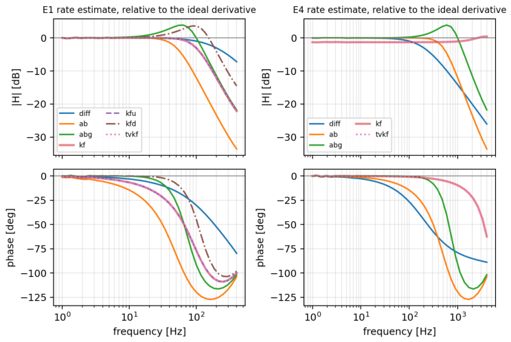
Figure 14.
C6’s coarse loop with each E1 estimator inside the executed kernel: crossover and modulus margin in the legend.
Figure 14.
C6’s coarse loop with each E1 estimator inside the executed kernel: crossover and modulus margin in the legend.
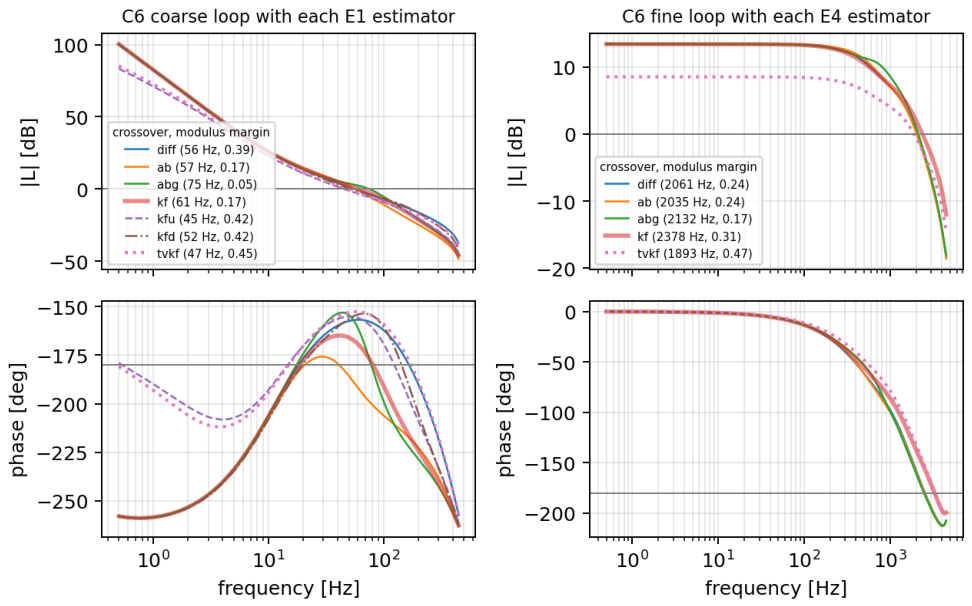
Figure 15.
Median optical error of every cell, per scenario, for C6 (left) and C1 (right).
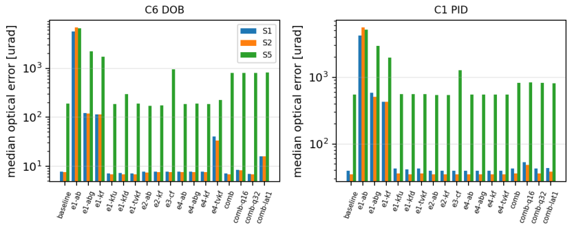
Figure 17.
F2, the wing crossing, advisory off (red) and on (green): true and predicted margin, bank, advisory urgency and acceptance, the terminal’s optical error (shaded where lock is lost) and the received power.
Figure 17.
F2, the wing crossing, advisory off (red) and on (green): true and predicted margin, bank, advisory urgency and acceptance, the terminal’s optical error (shaded where lock is lost) and the received power.
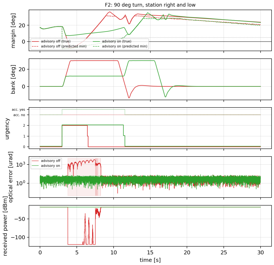
Figure 18.
Blocked time and held optical error per scenario, advisory off and on (medians over seeds).
Figure 18.
Blocked time and held optical error per scenario, advisory off and on (medians over seeds).
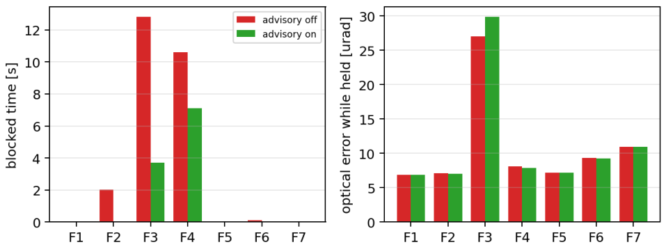
Table 1.
Principal mechanical and actuator parameters of the gimbal and the fast-steering mirror, with the origin tag of each value (CAD, datasheet, derived or assumed); the inertias and the structural mode come from the CAD assembly and its finite-element solve.
Table 1.
Principal mechanical and actuator parameters of the gimbal and the fast-steering mirror, with the origin tag of each value (CAD, datasheet, derived or assumed); the inertias and the structural mode come from the CAD assembly and its finite-element solve.
| Parameter | Value | Unit | Source |
|---|---|---|---|
| gimbal.J_AZ | 0.02573 | kg m2 | cad |
| gimbal.J_EL | 0.01291 | kg m2 | cad |
| gimbal.B_AZ | 0.012 | N m s/rad | assumed |
| gimbal.B_EL | 0.01 | N m s/rad | assumed |
| gimbal.tau_c_AZ | 0.008 | N m | assumed |
| gimbal.m_payload | 1.695 | kg | cad |
| gimbal.r_cg_EL | 0.03 | m | cad |
| gimbal.rate_limit | 6.283 | rad/s | assumed |
| gimbal.f_flex | 364 | Hz | cad |
| motor.tau_max | 4.05 | N m | datasheet |
| motor.Kt | 0.187 | N m/A | datasheet |
| motor.current_bw_hz | 800 | Hz | assumed |
| fsm.wn_hz | 1408 | Hz | derived |
| fsm.zeta | 0.6 | - | assumed |
| fsm.range_mech | 0.002 | rad | datasheet |
| fsm.optical_gain | 2 | - | assumed |
Sources: cad exported from the assembly, datasheet from a device datasheet, identified from measured data, assumed chosen for simulation only, TBD not yet known. The complete parameter set, and the origin of every entry, is in the released configuration; Table 3 summarises it.
Table 2.
Principal optical relay, detector and link parameters of the terminal model, with the origin tag of each value (datasheet, derived or assumed); the four-quadrant detector and the avalanche photodiode are named commercial parts.
Table 2.
Principal optical relay, detector and link parameters of the terminal model, with the origin tag of each value (datasheet, derived or assumed); the four-quadrant detector and the avalanche photodiode are named commercial parts.
| Parameter | Value | Unit | Source |
|---|---|---|---|
| relay.aperture_D | 0.04 | m | assumed |
| relay.eta_opt | 0.85 | - | assumed |
| relay.focal_qpd | 0.1 | m | assumed |
| relay.wavelength | 1.55e-06 | m | assumed |
| relay.split_apd | 0.7 | - | assumed |
| qpd.half_width | 0.0005 | m | datasheet |
| qpd.gap | 2e-05 | m | assumed |
| qpd.w_spot | 0.00012 | m | assumed |
| qpd.responsivity | 0.9 | A/W | datasheet |
| qpd.adc_bits | 14 | bit | assumed |
| apd.responsivity | 0.9 | A/W | datasheet |
| apd.gain_M | 10 | - | datasheet |
| apd.excess_noise_F | 4.5 | - | assumed |
| apd.required_snr_db | 15.6 | dB | assumed |
| link.range_m | 1000 | m | assumed |
| link.divergence | 0.002 | rad | assumed |
| link.p_rx_nominal | 2e-05 | W | assumed |
Table 3.
Origin of the whole parameter set: how many parameters carry each tag (CAD, datasheet, derived, assumed) and which policy each must satisfy before a result is reported.
Table 3.
Origin of the whole parameter set: how many parameters carry each tag (CAD, datasheet, derived, assumed) and which policy each must satisfy before a result is reported.
| Source | Count | % |
|---|---|---|
| cad | 7 | 8 |
| datasheet | 11 | 12 |
| derived | 4 | 5 |
| identified | 0 | 0 |
| assumed | 66 | 75 |
| TBD | 0 | 0 |
| total | 88 | 100 |
Parameters still TBD: none. patbench check-provenance –paper exits non-zero while any parameter is TBD or is assumed where the policy requires a measurement, and the table generator refuses to run unless that gate is explicitly overridden.
Table 4.
Tuning budget actually spent per controller family. Every searched family is given the same number of candidates, on the same training scenarios, with the same objective and the same feasibility screen; the training scenarios are disjoint from the test scenarios. The family’s analytic design is itself evaluated as one of those candidates, so no family can be reported with a configuration worse than its own published design.
Table 4.
Tuning budget actually spent per controller family. Every searched family is given the same number of candidates, on the same training scenarios, with the same objective and the same feasibility screen; the training scenarios are disjoint from the test scenarios. The family’s analytic design is itself evaluated as one of those candidates, so no family can be reported with a configuration worse than its own published design.
| Family | Dim. | Evaluations | Length [s] | Rejected | Obj.† | Selected |
|---|---|---|---|---|---|---|
| PID | 3 | 48 | 0.60 | 12 | 1.048 | searched |
| LQG | 9 | 48 | 0.60 | 36 | 1.700 | default |
| HINF | 8 | – | – | – | – | default |
| SMC | 8 | 48 | 0.60 | 38 | 0.189 | searched |
| ADRC | 4 | 48 | 0.60 | 9 | 0.734 | searched |
| DOB | 5 | 48 | 0.60 | 19 | 0.984 | searched |
Dim. is the number of free parameters searched. An equal evaluation budget is not an equal search budget: a fixed number of samples covers a three-parameter space far better than a seven-parameter one, which favours the more thinly parameterised families and must be read as a limitation of the protocol rather than a property of the methods. Rejected counts candidates discarded by the feasibility screen; they consume budget like any other evaluation. Selected states whether the search improved on the analytic design or that design survived its own budget. C3 is synthesised in closed form from its weights and is not searched, hence its empty row. †The objective is normalised against each family’s own first feasible evaluation, so it measures how much a family improved on its own starting point and is not comparable between rows: a lower value in one row does not mean that family tracks better. The value is the self-normalised total of the objective weights and indicates that the analytic design was the best candidate evaluated. Performance between families is compared in Section 3.1, on the test scenarios, and nowhere else.
Table 5.
The four estimation points of the terminal (E1–E4), the measurement and rate each receives, the simple estimator each ran in the control-law benchmark, and the candidates compared here.
Table 5.
The four estimation points of the terminal (E1–E4), the measurement and rate each receives, the simple estimator each ran in the control-law benchmark, and the candidates compared here.
| Point | Measurement, rate | Present estimator | Candidates |
|---|---|---|---|
| E1 gimbal rate | encoder, 1 , lsb | backward difference, low-pass 200 | -; --; steady-state KF; KF with torque input; disturbance-augmented KF; time-varying KF |
| E2 line of sight | optical error 50 , nav 50 | first-order correction, gain 0.8 | - on LOS; KF on LOS and LOS rate |
| E3 attitude | gyro 1 , AHRS | given (scenario model) | complementary filter (gyro integration corrected toward the AHRS) |
| E4 fine stage | QPD error 10 | backward difference, low-pass; ESO in C5; KF in C2 | -; --; steady-state KF; time-varying KF |
Table 6.
Operation count per execution (multiply-adds) and state memory, by variant and estimation point. n is the number of states.
Table 6.
Operation count per execution (multiply-adds) and state memory, by variant and estimation point. n is the number of states.
| Variant | Point (n) | Ops/tick | Mem. (words) | Rate |
|---|---|---|---|---|
| V- | E1 (2) | 6 | 2 | 1 |
| V2 steady KF | E1 (2) | 10 | 2 | 1 |
| V4 steady KF + input | E1 (2) | 14 | 2 | 1 |
| V6 disturbance-augmented | E1 (3) | 24 | 3 | 1 |
| V1 time-varying KF | E1 (2) | 2 + 3 | 1 | |
| V- | E2 (2 per axis) | 6 | 2 | 50 |
| V5 steady KF on LOS | E2 (2 per axis) | 10 | 2 | 50 |
| V7 complementary (two angles) | E3 (2) | 2 | 1 | |
| V- | E4 (2) | 6 | 2 | 10 |
| V-- | E4 (3) | 9 | 3 | 10 |
| V2 steady KF | E4 (2) | 10 | 2 | 10 |
| V1 time-varying KF (Joseph) | E4 (2) | 2 + 3 | 10 |
Table 7.
Data the terminal provides to the autopilot. The advisory is the only message that can change the flight path, and only if the autopilot’s arbitration accepts it.
Table 7.
Data the terminal provides to the autopilot. The advisory is the only message that can change the flight path, and only if the autopilot’s arbitration accepts it.
| Message | Fields | Rate | Meaning |
|---|---|---|---|
| link status | mode, lock, optical error, | 20 | for logging, for the ground |
| field of regard | m, , nearest edge id | 20 | how much room is left |
| advisory | turn direction, bank limit , course preference , urgency , | 20 | what would keep the link, for the autopilot to weigh |
Table 8.
The experiment matrix. Each cell is run with C6 and with C1 on three scenarios and eight paired seeds.
Table 8.
The experiment matrix. Each cell is run with C6 and with C1 on three scenarios and eight paired seeds.
| Stage | Variation | Cells |
|---|---|---|
| base | present estimators | 1 |
| K-A | E1 ∈ {, , KF, KF+input, KF+dist., TV-KF} | 6 |
| K-B | E2 ∈ {, KF} | 2 |
| K-C | E3 ∈ {complementary} | 1 |
| K-D | E4 ∈ {, , KF, TV-KF} | 4 |
| K-E | best of K-A..K-D combined | 1 |
| K-F | K-E with Q15 and Q31 state storage | 2 |
| K-G | K-E with one tick of estimator latency | 1 |
| 18 cells × 2 laws × 3 scenarios × 8 seeds | 864 runs | |
| plus cold-start acquisition, 2 cells × 2 laws × 8 seeds | 32 runs |
Table 9.
Verification steps 1–2 of the fixed-wing flight study: trim, linear modes, nonlinear-versus-linear elevator doublet, autopilot turn.
Table 9.
Verification steps 1–2 of the fixed-wing flight study: trim, linear modes, nonlinear-versus-linear elevator doublet, autopilot turn.
| Check | Result |
|---|---|
| trim at 25 / | 4.71 deg, -6.26 deg, throttle 0.33, residual 7e-14 |
| short period | 3.88 rad/s, 0.36 |
| phugoid | 0.52 rad/s, 0.48 |
| Dutch roll | 9.78 rad/s, 0.40 |
| roll / spiral | -11.4 / - |
| doublet, nonlinear vs linear | q 0.5 %, 0.5 % of peak (RMS) |
| autopilot, 120 deg turn at 30 deg bank | 10.2 s, overshoot 2.5 deg, altitude 999.1–1000.7 m |
Table 10.
The seven fixed-wing flight scenarios F1–F7. All are flown at 25/, starting at the origin heading north, with the ground station at the stated position; each is flown with the advisory off and on over 8 seeds, and the terminal (C6 on both stages, the present estimators) is driven through every flight. The third column names the edge of the field of regard each scenario is designed to reach.
Table 10.
The seven fixed-wing flight scenarios F1–F7. All are flown at 25/, starting at the origin heading north, with the ground station at the stated position; each is flown with the advisory off and on over 8 seeds, and the terminal (C6 on both stages, the present estimators) is driven through every flight. The third column names the edge of the field of regard each scenario is designed to reach.
| Id | Flight | What it tests |
|---|---|---|
| F1 | straight and level at 1000 , station ahead-right, 20 | control: the link must never leave the region |
| F2 | right turn at bank commanded at 3 , station at azimuth , elevation , 30 | the right wing crosses the line of sight during the bank |
| F3 | straight overflight of the station at 400 , 32 | the lock cone at nadir, then the tail |
| F4 | right turn at 3 , station 2 ahead, 25 | the flight plan puts the station behind the tail |
| F5 | two UAVs crossing at 200 height difference, both on autopilots, 25 | both terminals advise; the symmetric case |
| F6 | F2 with a 10 / crosswind and light Dryden turbulence; terminal in the vibration environment S2 | wind in the prediction, vibration in the loop |
| F7 | loiter of 150 radius at 400 with the station inside the circle, 40 | continuous bank towards the partner |
Table 11.
The quadrotor: parameters with their origin, and the verification checks of steps 1–2.
| Quantity | Value | Source |
|---|---|---|
| empty mass | datasheet | |
| max take-off / payload | 34.86 / | datasheet |
| motor circle, propeller | 1415, 33 in | datasheet |
| thrust-to-weight (no payload) | 2.5 | datasheet |
| max speed, max wind | 26, 10 / | datasheet |
| payload | this study | |
| battery, motors | 4.0, 4 × | assumed |
| motor lag, torque/thrust | 80, | assumed |
| drag area | assumed; gives 48 deg at 26 m/s | |
| flying mass | derived | |
| inertia | 1.34, 1.34, | derived from the mass layout |
| hover throttle | 0.51 of max thrust | derived |
| velocity step 0 → 10 / | 2.7 s to 9.5 m/s, cruise tilt 9.4 deg | check |
| yaw | 2.8 s | check (rate limit /) |
| hover in 10 / wind | tilt 9.4 deg (analytic 9.4) | check |
| altitude through all of the above | 99.1– | check |
Table 13.
Nominal tracking performance (Series A), pooled over scenarios S1 and S2 with no plant uncertainty.
Table 13.
Nominal tracking performance (Series A), pooled over scenarios S1 and S2 with no plant uncertainty.
| Controller | [] | [] | [] | [] | TV | [] | |||
|---|---|---|---|---|---|---|---|---|---|
| C1 PID | 39.7 [29.2, 43.1] | 71.0 [51.4, 76.3] | 1048 | 0.579 | 883 | 1117 | 1.00 | 0.000 | 0.00 |
| C2 LQG | 62.1 [47.3, 67.9] | 109.5 [82.3, 128.8] | 966 | 0.534 | 247 | 1009 | 1.00 | 0.000 | 0.00 |
| C | – | – | – | – | – | – | 0.01 | 0.983 | 1.00 |
| C4 SMC | 469.1 [465.0, 474.5] | 781.4 [770.4, 834.7] | 653 | 0.649 | 1506 | 673 | 0.97 | 0.007 | 0.38 |
| C5 ADRC | 113.3 [94.3, 134.0] | 203.1 [163.4, 265.0] | 896 | 0.550 | 503 | 969 | 1.00 | 0.000 | 0.00 |
| C6 DOB | 7.6 [7.4, 8.1] | 13.4 [12.8, 14.1] | 743 | 0.604 | 811 | 945 | 1.00 | 0.000 | 0.00 |
| C7 hybrid | 7.6 [7.4, 8.1] | 13.4 [12.8, 14.1] | 743 | 0.604 | 811 | 945 | 1.00 | 0.000 | 0.00 |
Table 14.
The reference plant (P1) against a second plant (P2) with payload mass and inertia doubled: median optical error and two-stage rejection on the nominal series.
Table 14.
The reference plant (P1) against a second plant (P2) with payload mass and inertia doubled: median optical error and two-stage rejection on the nominal series.
| Controller | [] | Rejection | ||
|---|---|---|---|---|
| P1 | P2 | P1 | P2 | |
| C1 PID | 39.7 | 39.5 | 26.4 | 26.5 |
| C2 LQG | 62.1 | 72.3 | 15.6 | 14.5 |
| C4 SMC | 469.7 | 538.1 | 1.4 | 1.8 |
| C5 ADRC | 113.3 | 113.5 | 7.9 | 7.9 |
| C6 DOB | 7.6 | 7.1 | 97.1 | 105.9 |
Rejection is coarse residual over optical error. C3 fails on both plants. Medians of Series A runs with feed-forward and both stages on and failed runs excluded, hence the small differences from Table 13. The four tests stated before the second plant was run (P1–P4 here; named H1–H4 in the released code and Supplementary Report S1, not to be confused with the estimator tests) all pass.
Table 15.
Performance of each controller family in the manual-pointing (Series P) and cold-start acquisition (Series Q) modes: manual-pointing error, time to first lock, lock losses and reacquisition time, medians over eight seeds. Acquisition speed is only weakly predicted by tracking accuracy.
Table 15.
Performance of each controller family in the manual-pointing (Series P) and cold-start acquisition (Series Q) modes: manual-pointing error, time to first lock, lock losses and reacquisition time, medians over eight seeds. Acquisition speed is only weakly predicted by tracking accuracy.
| Controller | Manual [] | [s] | [s] | ||
|---|---|---|---|---|---|
| C1 PID | 4615 [3420, 5767] | 1.57 [1.07, 3.18] | 0.0 | – | 0.79 |
| C2 LQG | 4598 [3474, 5744] | 0.85 [0.58, 1.26] | 0.0 | 3.86 [3.82, 3.89] | 0.86 |
| C | 741721 [738531, 745070] | – | 0.0 | – | 0.00 |
| C4 SMC | 4606 [3479, 5748] | 1.43 [0.90, 5.16] | 2.0 | 1.16 [0.86, 2.66] | 0.08 |
| C5 ADRC | 4596 [3463, 5718] | 1.03 [0.77, 1.25] | 1.5 | 1.77 [1.24, 2.32] | 0.51 |
| C6 DOB | 4536 [3451, 5678] | 0.87 [0.65, 1.23] | 0.0 | 0.78 [0.78, 0.78] | 0.86 |
| C7 hybrid | 4598 [3474, 5744] | 0.85 [0.58, 1.26] | 0.0 | 2.45 [1.78, 3.12] | 0.86 |
Manual pointing runs open-loop with the fine stage parked, so its error is set by the navigation and attitude estimates rather than by the optical loop. is measured from the moment the search starts.
Table 16.
The estimator matrix: median optical error over eight paired seeds, in , for C6 and C1 on the three tracking scenarios, with the failure probability where it is not zero. The estimation error of the varied point is given for C6 on S2 (E1 in , E2 and E3 in ).
Table 16.
The estimator matrix: median optical error over eight paired seeds, in , for C6 and C1 on the three tracking scenarios, with the failure probability where it is not zero. The estimation error of the varied point is given for C6 on S2 (E1 in , E2 and E3 in ).
| Series | Cell | C6: S1 / S2 / S5 | C1: S1 / S2 / S5 | Est. err. | C6 S5 | ||||
|---|---|---|---|---|---|---|---|---|---|
| base | present | 7.7 | 7.6 | 191.7 | 39.9 | 34.9 | 553.0 | 38.21 | 0.25 |
| K-A | E- | 5667.0 | 6804.3 | 6564.1 | 4226.3 | 5585.8 | 5180.1 | 1482.11 | 1.00 |
| K-A | E-- | 121.5 | 120.3 | 2248.6 | 587.2 | 511.0 | 2981.5 | 1062.94 | 0.50 |
| K-A | E1 KF | 114.2 | 114.5 | 1725.8 | 427.5 | 426.6 | 1971.7 | 713.94 | 0.38 |
| K-A | E1 KF+input | 7.1 | 6.8 | 187.9 | 42.7 | 36.1 | 562.8 | 51.76 | 0.25 |
| K-A | E1 KF+dist. | 7.2 | 6.9 | 299.3 | 41.2 | 35.1 | 557.8 | 26.66 | 0.25 |
| K-A | E1 TV-KF | 7.1 | 6.8 | 189.0 | 42.6 | 35.9 | 562.5 | 51.84 | 0.25 |
| K-B | E- | 7.7 | 7.5 | 171.4 | 39.7 | 34.9 | 544.6 | 1115 | 0.25 |
| K-B | E2 KF | 7.7 | 7.6 | 174.7 | 39.8 | 34.9 | 544.2 | 1111 | 0.25 |
| K-C | E3 compl. | 7.7 | 7.5 | 949.8 | 39.9 | 35.1 | 1279.0 | 1095 | 0.12 |
| K-D | E- | 7.8 | 7.5 | 185.8 | 39.9 | 34.9 | 553.0 | – | 0.25 |
| K-D | E-- | 7.8 | 7.7 | 192.2 | 39.9 | 34.9 | 553.0 | – | 0.25 |
| K-D | E4 KF | 7.8 | 7.6 | 186.5 | 39.9 | 34.9 | 553.0 | – | 0.25 |
| K-D | E4 TV-KF | 40.7 | 33.7 | 224.8 | 39.9 | 34.9 | 553.0 | – | 0.25 |
| K-E | combined best | 7.1 | 6.8 | 801.6 | 42.6 | 36.2 | 824.4 | – | 0.12 |
| K-F | combined, Q15 | 8.5 | 8.2 | 802.2 | 52.9 | 48.2 | 845.4 | – | 0.12 |
| K-F | combined, Q31 | 7.0 | 6.8 | 800.3 | 42.6 | 36.2 | 824.5 | – | 0.12 |
| K-G | combined, 1-tick latency | 16.1 | 15.8 | 817.5 | 43.3 | 38.5 | 816.7 | – | 0.00 |
Table 17.
The six tests of the estimator benchmark (H1–H6, stated before the runs in Section 2.13) with their outcome and the measured quantity each was decided on.
Table 17.
The six tests of the estimator benchmark (H1–H6, stated before the runs in Section 2.13) with their outcome and the measured quantity each was decided on.
| Test | Outcome | Measured |
|---|---|---|
| H1 | fail | largest E1 change on C6 nominal 80940 % |
| H2 | fail | present 0.25, best E1 0.25 |
| H3 | fail | best E4 change on C6 nominal -1 % |
| H4 | pass | largest E2 change 1 % |
| H5 | pass | Q31 -0.2 %, Q15 +20 % |
| H6 | pass | one tick of latency +130 % |
Table 20.
Every flight scenario with the advisory off and on: medians over 8 seeds. Blocked: time the required direction is outside the usable region; P(bl.): fraction of seeds with any blockage; lead: first warning before the first blockage; held: optical RMS while the link is usable and locked, excluding the half second after each re-lock; drops: lock losses while the direction is usable; turn: time from the course command to capture; acc./bl./ov.: advisories accepted, blended, overridden.
Table 20.
Every flight scenario with the advisory off and on: medians over 8 seeds. Blocked: time the required direction is outside the usable region; P(bl.): fraction of seeds with any blockage; lead: first warning before the first blockage; held: optical RMS while the link is usable and locked, excluding the half second after each re-lock; drops: lock losses while the direction is usable; turn: time from the course command to capture; acc./bl./ov.: advisories accepted, blended, overridden.
| Flight | Adv. | Blocked [s] | P(bl.) | Lead [s] | Held [] | Lock | Drops | Turn [s] | acc./bl./ov. |
|---|---|---|---|---|---|---|---|---|---|
| F1 | off | 0.0 | 0.00 | – | 6.9 | 1.000 | 0 | 0.0 | 0/0/0 |
| on | 0.0 | 0.00 | – | 6.9 | 1.000 | 0 | 0.0 | 0/0/0 | |
| F2 | off | 2.0 | 1.00 | 0.8 | 7.1 | 0.844 | 4 | 7.7 | 0/0/0 |
| on | 0.0 | 0.00 | – | 7.0 | 1.000 | 0 | 12.8 | 171/0/0 | |
| F3 | off | 12.8 | 1.00 | 6.6 | 27.0 | 0.408 | 1 | 0.0 | 0/0/0 |
| on | 3.7 | 1.00 | 6.7 | 29.8 | 0.431 | 8 | 0.0 | 0/295/91 | |
| F4 | off | 10.6 | 1.00 | 5.6 | 8.1 | 0.576 | 0 | 13.4 | 0/0/0 |
| on | 7.1 | 1.00 | 9.1 | 7.8 | 0.715 | 0 | 16.8 | 137/0/188 | |
| F5 | off | 0.0 | 0.00 | – | 7.2 | 1.000 | 0 | 0.0 | 0/0/0 |
| on | 0.0 | 0.00 | – | 7.2 | 1.000 | 0 | 0.0 | 0/0/0 | |
| F6 | off | 0.1 | 0.50 | 0.8 | 9.4 | 0.896 | 3 | 6.0 | 0/0/0 |
| on | 0.0 | 0.00 | – | 9.3 | 0.896 | 2 | 7.8 | 66/0/0 | |
| F7 | off | 0.0 | 0.00 | – | 10.9 | 0.802 | 11 | 2.1 | 0/0/0 |
| on | 0.0 | 0.00 | – | 10.9 | 0.802 | 11 | 2.1 | 0/0/0 |
Table 21.
The seven tests of the fixed-wing flight study (T1–T7, stated before the runs in Section 2.14) with their outcome and the measured quantity each was decided on; where a test has two clauses, both outcomes are given.
Table 21.
The seven tests of the fixed-wing flight study (T1–T7, stated before the runs in Section 2.14) with their outcome and the measured quantity each was decided on; where a test has two clauses, both outcomes are given.
| Test | Result | Detail |
|---|---|---|
| T1 | pass | min lock fraction 1.000 |
| T2 | fail | link pass (8/8 kept), turn-time cost +65 % (fail) |
| T3 | pass | lead pass (min 6.5 s), blocked 12.8 → 3.7 s (pass) |
| T4 | fail | 137 of 325 advisories accepted, 0 blended, 188 overridden (the clause `none accepted’ fails) |
| T5 | pass | max 0.0 WARN toggles per minute |
| T6 | fail | link pass (8/8 kept), held error 9.3 vs S (fail) |
| T7 | pass | min margin 9.0 deg, no advisory |
Table 22.
Every quadrotor flight with the advisory off and on: medians over 8 seeds; columns as in Table 20.
Table 22.
Every quadrotor flight with the advisory off and on: medians over 8 seeds; columns as in Table 20.
| Flight | Adv. | Blocked [s] | P(bl.) | Lead [s] | Held [] | Lock | Drops | Turn [s] | acc./bl./ov. |
|---|---|---|---|---|---|---|---|---|---|
| Q1 | off | 0.0 | 0.00 | – | 6.8 | 1.000 | 0 | 0.0 | 0/0/0 |
| on | 0.0 | 0.00 | – | 6.8 | 1.000 | 0 | 0.0 | 0/0/0 | |
| Q2 | off | 15.3 | 1.00 | 0.2 | 6.8 | 0.169 | 8 | 0.0 | 0/0/0 |
| on | 0.0 | 0.00 | – | 6.8 | 1.000 | 0 | 0.0 | 340/0/0 | |
| Q3 | off | 9.8 | 1.00 | 5.7 | 16.5 | 0.568 | 1 | 0.0 | 0/0/0 |
| on | 4.5 | 1.00 | 5.7 | 16.5 | 0.568 | 1 | 0.0 | 122/0/188 | |
| Q4 | off | 0.5 | 1.00 | 0.9 | 6.8 | 0.746 | 2 | 3.1 | 0/0/0 |
| on | 0.5 | 1.00 | 0.9 | 6.8 | 0.746 | 2 | 3.1 | 0/0/55 | |
| Q5 | off | 15.6 | 1.00 | 0.0 | 40.6 | 0.108 | 9 | 0.0 | 0/0/0 |
| on | 4.6 | 1.00 | 0.0 | 59.9 | 0.000 | 1 | 0.0 | 205/0/295 | |
| Q6 | off | 0.0 | 0.00 | – | 6.8 | 1.000 | 0 | 0.0 | 0/0/0 |
| on | 0.0 | 0.00 | – | 6.8 | 1.000 | 0 | 0.0 | 0/0/0 | |
| Q7 | off | 0.0 | 0.00 | – | 6.7 | 1.000 | 0 | 39.7 | 0/0/0 |
| on | 0.0 | 0.00 | – | 6.7 | 1.000 | 0 | 39.7 | 0/0/0 |
Table 23.
The seven tests of the quadrotor study (QT1–QT7, stated before the runs in Section 2.15) with their outcome and the measured quantity each was decided on.
Table 23.
The seven tests of the quadrotor study (QT1–QT7, stated before the runs in Section 2.15) with their outcome and the measured quantity each was decided on.
| Test | Result | Detail |
|---|---|---|
| QT1 | pass | min lock fraction 1.000 |
| QT2 | pass | link pass (8/8 kept), cruise speed 61 % of commanded (pass) |
| QT3 | pass | lead pass (min 5.6 s), blocked 9.8 → 4.5 s (pass) |
| QT4 | pass | blocked at most 0.51 s, lead at least 0.9 s |
| QT5 | pass | blocked 15.6 → 4.6 s, max 0.0 toggles/min |
| QT6 | pass | link pass, held error 6.8 vs S (pass), tilt 18.7 deg |
| QT7 | pass | never blocked; lock fraction 1.000; min margin 6.6 deg |
Table 24.
Link availability and delivered data per flight, advisory off and on: availability is the median over eight seeds of the fraction of the flight with the required direction inside the field of regard and the terminal locked; data is availability times duration times the modelled 1/ rate, without coding or protocol overhead; the last row sums the seven flights.
Table 24.
Link availability and delivered data per flight, advisory off and on: availability is the median over eight seeds of the fraction of the flight with the required direction inside the field of regard and the terminal locked; data is availability times duration times the modelled 1/ rate, without coding or protocol overhead; the last row sums the seven flights.
| Fixed wing | Quadrotor | ||||||||||
|---|---|---|---|---|---|---|---|---|---|---|---|
| Flight | Dur. [s] | Advisory off | Advisory on | Flight | Dur. [s] | Advisory off | Advisory on | ||||
| Av. [%] | Gbit | Av. [%] | Gbit | Av. [%] | Gbit | Av. [%] | Gbit | ||||
| F1 | 20 | 100.0 | 20.0 | 100.0 | 20.0 | Q1 | 20 | 100.0 | 20.0 | 100.0 | 20.0 |
| F2 | 30 | 84.4 | 25.3 | 100.0 | 30.0 | Q2 | 20 | 16.9 | 3.4 | 100.0 | 20.0 |
| F3 | 32 | 40.8 | 13.1 | 43.1 | 13.8 | Q3 | 30 | 56.8 | 17.0 | 56.8 | 17.0 |
| F4 | 25 | 57.6 | 14.4 | 71.5 | 17.9 | Q4 | 20 | 74.6 | 14.9 | 74.6 | 14.9 |
| F5 | 25 | 100.0 | 25.0 | 100.0 | 25.0 | Q5 | 25 | 10.8 | 2.7 | 0.0 | 0.0 |
| F6 | 30 | 89.6 | 26.9 | 89.6 | 26.9 | Q6 | 25 | 100.0 | 25.0 | 100.0 | 25.0 |
| F7 | 40 | 80.2 | 32.1 | 80.2 | 32.1 | Q7 | 40 | 100.0 | 40.0 | 100.0 | 40.0 |
| sum | 202 | 157 | 166 | sum | 180 | 123 | 137 | ||||
Disclaimer/Publisher’s Note: The statements, opinions and data contained in all publications are solely those of the individual author(s) and contributor(s) and not of MDPI and/or the editor(s). MDPI and/or the editor(s) disclaim responsibility for any injury to people or property resulting from any ideas, methods, instructions or products referred to in the content. |
© 2026 by the authors. Licensee MDPI, Basel, Switzerland. This article is an open access article distributed under the terms and conditions of the Creative Commons Attribution (CC BY) license (http://creativecommons.org/licenses/by/4.0/).
Copyright: This open access article is published under a Creative Commons CC BY 4.0 license, which permit the free download, distribution, and reuse, provided that the author and preprint are cited in any reuse.