
Submitted:
14 November 2026
Posted:
17 November 2026
You are already at the latest version
Abstract
Frosty pod rot, caused by Moniliophthora roreri, is the main disease of cacao in the Ecuadorian Amazon, where fungicide use is rising without sensitivity baselines. We measured the mycelial growth of 23 single-spore isolates from six farms in Orellana Province on media amended with azoxystrobin, boscalid, difenoconazole or copper sulfate (0.01–100 µg mL−1) and estimated EC50 values. Difenoconazole was the most active (geometric mean 0.32 µg mL−1). Boscalid gave a narrow distribution (1.02 µg mL−1) apart from three slow-growing isolates. Copper sulfate did not halve the growth of any isolate at 100 µg mL−1. Azoxystrobin split the collection into 11 sensitive isolates (0.035 µg mL−1) and 12 less sensitive ones (1.00 µg mL−1), with none in between (mixture model, p = 0.002). The less sensitive isolates came mostly from a commercial CCN51 farm and a Nacional farm, and isolates from the same field sample behaved alike. A principal component analysis of the growth profiles, run without prior grouping, placed azoxystrobin on the first axis (35.1% of the variance). Twenty-three isolates suffice as provisional baselines for difenoconazole and boscalid; azoxystrobin needs about 120 farm-stratified isolates to detect a threefold shift. These are in vitro phenotypes; resistance has not been demonstrated.
Keywords:
frosty pod rot
; Theobroma cacao
; EC50
; baseline sensitivity
; QoI fungicides
; azoxystrobin
; copper
; population structure
; principal component analysis
; Monte Carlo simulation
1. Introduction
Frosty pod rot attacks the fruit of cacao (Theobroma cacao L.). Its agent, the basidiomycete Moniliophthora roreri (Cif.) H.C. Evans, Stalpers, Samson & Benny, infects pods while they are small and stays latent for several weeks. Then the pods rot and become covered by a cream-coloured mat of spores [1,2,3]. One diseased pod releases enormous numbers of spores, wind and rain carry them to the next cohort of fruits, and in unmanaged plantings the disease can take most of the harvest [1,2]. The fungus belongs to the Marasmiaceae, next to M. perniciosa, which causes witches’ broom [4].
For most of the twentieth century the pathogen stayed in north-western South America. It has since reached Central America, Mexico, Peru and Bolivia, and its spread has followed the expansion of cacao growing closely [1,5]. Its genetic diversity peaks in Colombia [6]. Cacao was first used and domesticated in the upper Amazon of south-eastern Ecuador about 5300 years ago [7], and that region still holds much of the genetic variation of the species [8]. Orellana Province lies in its northern part. Cacao is now one of the province’s main cash crops, grown as the fine-flavour Nacional type, the high-yielding clone CCN51 and a local selection called Súper Árbol, and frosty pod rot is present in all of them [9].
Growers still rely mostly on cultural control. They remove diseased pods at short intervals and regulate shade and prune to lower inoculum and canopy humidity [2,10,11]. Many smallholders cannot pay for that much labour, so they turn to fungicides, traditionally copper. In Mexico, one application of azoxystrobin, trifloxystrobin, tebuconazole or propiconazole combined with monthly copper hydroxide sprays reduced disease incidence in the field [12]. In Ecuador, azoxystrobin and copper sulfate have been tested in vitro and in spray programmes [13,14].
Single-site fungicides carry a cost. The Fungicide Resistance Action Committee (FRAC) rates the quinone outside inhibitors (QoIs, FRAC group 11) as high-risk, the succinate dehydrogenase inhibitors (SDHIs, group 7) as medium- to high-risk and the demethylation inhibitors (DMIs, group 3) as medium-risk [15,16]. To manage that risk one needs to know how sensitive the population was before selection began, which means a baseline distribution against which later samples can be compared [17,18]. For M. roreri such data are thin. The largest survey so far tested 76 Ecuadorian isolates against azoxystrobin and found all of them highly sensitive [19]. Another Ecuadorian study used two isolates [13]. We found no population data for an SDHI or a DMI, and no study that tested several modes of action on the same Amazonian isolates.
A list of EC50 values does not make a baseline by itself. M. roreri reproduces clonally [20], so isolates from the same pod, tree or farm may be copies of one clone, and a collection can look larger than it is. If sensitivity differs among farms, a provincial mean can hide a subpopulation that has already shifted.
We set out to describe the in vitro sensitivity of 23 M. roreri isolates from Orellana Province to azoxystrobin, boscalid, difenoconazole and copper sulfate, working from the full plate-level growth data. We also tested whether sensitivity was structured by farm, canton or cacao genotype, and used resampling and simulation to estimate how many isolates a baseline for each fungicide would need.
2. Materials and Methods
2.1. Study Area and Isolates
The isolates came from the three cantons of Orellana Province, Ecuador, and were sampled in the same project as our survey of cacao fruit endophytes [9]. Loreto lies at 0°47′28″ S, 77°22′19″ W and 373 m a.s.l. (mean temperature 23.6 °C, relative humidity 81–89%, annual rainfall 2516 mm), Francisco de Orellana at 0°37′36″ S, 77°07′40″ W and 292 m a.s.l. (26 °C; 86–89%; 2800–4500 mm), and La Joya de los Sachas at 0°45′41″ S, 77°05′01″ W and 330 m a.s.l. (25 °C; 90%; 4534 mm). Pods with symptoms of frosty pod rot were collected in five sampling rounds between June 2021 and May 2022 on six farms (Table 1). La Belleza is in Francisco de Orellana, and La Paz and Bajo Huiruno are in the parish of Puerto Murialdo. La Calumeña (Lago San Pedro), Unión Milagreña and San Carlos (parish of San Carlos) are in Joya de los Sachas. The trees were CCN51, Súper Árbol or Nacional. The isolates were obtained from the symptomatic pods collected on these farms at the Plant Pathology Laboratory of the Escuela Superior Politécnica de Chimborazo (ESPOCH), Riobamba, where they were also characterized and assayed.
Spores were taken from sporulating lesions with a sterile syringe and plated on potato dextrose agar (PDA; 39 g L−1; Difco, Becton, Dickinson and Company, Franklin Lakes, NJ, USA), which was incubated at 28 °C in the dark. After 10 days, colonies were purified by successive transfers until single-spore cultures were obtained. These were preserved in sterile distilled water by the Castellani method at 4–8 °C [9,21]. Isolates were identified from symptoms, culture characters and morphology. Diseased pods showed the internal necrosis and cream-coloured sporulating mat typical of frosty pod rot [1,2]. Colonies were described by mycelial colour on the obverse and reverse, recorded with the Pantone Color Matching System, and by margin shape, texture and elevation. Adhesive-tape mounts in lactoglycerol [22], examined under a Leica DML microscope, showed chains of globose to ellipsoid spores [2,3]. No molecular identification was performed.
Twenty-three isolates (C1–C23) were retained. Thirteen came from Joya de los Sachas, 8 from Francisco de Orellana and 2 from Loreto; 9 were from CCN51, 8 from Súper Árbol and 6 from Nacional trees. Seven pairs of isolates shared a field sample, so the collection represents 16 field samples, and the analysis took the pairing into account (Section 2.6).
2.2. Fungicides and Amended Media
Four fungicides with different modes of action were tested (Table 2) [15]. They were azoxystrobin (QoI; FRAC group 11), boscalid (SDHI; group 7), difenoconazole (DMI; group 3) and copper sulfate, used as copper sulfate pentahydrate (CuSO4·5H2O; inorganic multisite; group M01). All four were commercial products: Amistar® 50 WG (azoxystrobin 500 g kg−1, water-dispersible granules; Syngenta, Basel, Switzerland), Cantus® (boscalid 500 g kg−1, WG; BASF, Ludwigshafen, Germany), Score® 250 EC (difenoconazole 250 g L−1, emulsifiable concentrate; Syngenta) and Phyton® 27 (CuSO4·5H2O 240 g L−1, soluble concentrate; Phyton Corp., Bloomington, MN, USA). Concentrations refer to the active ingredient and, for copper, to the pentahydrate salt, of which metallic copper makes up about 25% (molar mass 249.7 g mol−1; Cu 63.55 g mol−1). A stock solution of 10 000 µg mL−1 of active ingredient (for copper, of copper sulfate pentahydrate) was prepared in sterile distilled water. It was diluted 1:2 and then serially 1:10 to obtain working solutions of 5000, 500, 50, 5 and 0.5 µg mL−1. Following Mihajlović et al. [23], 0.918 mL of the corresponding working solution was added to 45 mL of molten PDA to give final concentrations of 100, 10, 1, 0.1 and 0.01 µg mL−1. Fifteen millilitres were dispensed into each of three 90 mm Petri dishes per concentration. Control plates (0 µg mL−1) were prepared without fungicide.
2.3. Mycelial Growth Assays
Each fungicide was tested as a separate experiment with all 23 isolates, six concentrations and three replicate plates per concentration. The plate was the experimental unit. Plates were sown on 17 August 2022 (azoxystrobin), 22 August (boscalid), 27 August (copper sulfate) and 12 September 2022 (difenoconazole). Mycelial discs 5.8 mm in diameter were cut with sterile drinking straws from the margin of actively growing colonies and placed on the amended plates, which were incubated in the dark at 27 ± 2 °C. Two perpendicular colony diameters were measured at 48, 72, 96 and 120 h, and growth was calculated as the mean diameter minus the disc diameter. The data set holds 6624 records, with 36 missing diameters.
Three variables were derived for each plate. The mycelial growth rate (MGR, mm day−1) was the slope of a linear regression of growth on time between days 2 and 5. The area under the mycelial growth curve (AUMGC, mm·day) was computed from 48 to 120 h by the trapezoidal rule, by analogy with the area under the disease progress curve [24]. Relative AUMGC was the AUMGC of each plate as a percentage of the mean of the control plates of the same isolate.
2.4. Analysis of Growth
Differences in vigour among isolates were tested with the Kruskal–Wallis test on the AUMGC of the control plates. For each fungicide, relative AUMGC was analysed as a randomized complete block design, with concentration as the treatment and isolate as the block (n = 23), and means were separated with Tukey’s HSD test (α = 0.05). The same design, with fungicide as the treatment, compared the four fungicides at each concentration; the Friedman test was run alongside as a nonparametric check. Within each isolate, a one-way ANOVA of AUMGC on concentration (three plates per concentration) followed by Tukey’s test showed whether that isolate responded at all. The effects of canton and cacao genotype on relative AUMGC averaged over concentrations were examined with the Kruskal–Wallis test.
2.5. EC50 Estimation
For each isolate and fungicide, log-logistic models were fitted to the MGR of the 18 plates with the R package drc [25]. The default was the three-parameter model with the lower limit fixed at zero (LL.3), whose parameter e is the EC50. The four-parameter model (LL.4) replaced it when its Akaike information criterion (AIC) was at least two units lower. With LL.4 the absolute EC50 is reported, that is, the concentration at which the fitted curve falls to half of its upper limit. For azoxystrobin, LL.4 and the absolute EC50 were used for all 23 isolates, because inhibition levelled off at a partial plateau, the residual growth often seen when QoIs are tested on mycelium [26]. The 95% confidence interval of each EC50 was a bootstrap percentile interval. Plates were resampled with replacement within each concentration, the model was refitted 300 times, and resamples that failed to converge were discarded. The delta-method intervals from drc are reported as well (Table S1). EC50 values were not extrapolated. Isolates whose mean inhibition at 100 µg mL−1 was below 50% were recorded as >100 µg mL−1, and estimates below 0.01 µg mL−1 as <0.01 µg mL−1. Recomputing the LL.3 fits with the ec50estimator package [27] returned the same estimates for every isolate. EC50 values were also calculated from the 120-h diameter (Table S1).
Isolates were placed in descriptive categories adapted from Gudmestad et al. [28] and consistent with the general criterion of Edgington et al. [29]. The classes were highly sensitive (HS; EC50 < 1 µg mL−1), sensitive (S; 1–5 µg mL−1), moderately sensitive (MS; >5–20 µg mL−1), low sensitivity (LS; >20–100 µg mL−1) and very low sensitivity (VLS; >100 µg mL−1). Gudmestad et al. called the third and fourth classes moderately and highly resistant, but they set those limits for SDHIs in Alternaria solani, and the limits have no validated meaning for M. roreri. Here they are used only as a common scale.
2.6. Population Analysis
For each single-site fungicide, log10 EC50 was described by a normal distribution fitted by maximum likelihood with interval censoring (survreg, log-normal) [30,31]. The geometric mean (GM), the geometric standard deviation (GSD) and the 95th and 99th percentiles (P95, P99) were derived from the fit. Isolates from one field sample are not independent, so 95% confidence intervals came from a cluster bootstrap that resampled the 16 field samples with replacement (1000 replicates) [32,33]. Normality of log10 EC50 was checked with the Shapiro–Wilk test.
Fungicides were compared on the same isolates with the Friedman test and with pairwise Wilcoxon signed-rank tests on log10 EC50, adjusted by Holm’s method [34]. Cross-sensitivity was assessed with Spearman correlations among log10 EC50 values and copper inhibition at 100 µg mL−1. Effects of canton, cacao genotype and farm were tested with the Kruskal–Wallis test. Each farm grew mainly one cacao genotype, so cacao genotype and farm are confounded in this collection, and every test involving cacao genotype is read as descriptive. To test whether isolates from one field sample were alike, the mean absolute difference in log10 EC50 within the seven same-sample pairs was compared with its distribution over 5000 random pairings of the 23 isolates.
The azoxystrobin values appeared to fall into two groups, so a two-component normal mixture was fitted to log10 EC50 (censored values entered as 0.005 µg mL−1) with the expectation–maximization algorithm of mixtools [35]. It was compared with a single normal distribution by the likelihood ratio (LR). The null distribution of the LR came from a parametric bootstrap of 500 data sets simulated under the single normal [36], and the Bayesian information criterion (BIC) was compared as well. Each isolate was assigned to the component with the higher posterior probability. Association of the resulting phenotypes with farm, canton and cacao genotype was tested with chi-square tests whose p-values were obtained by Monte Carlo simulation (20,000 replicates).
To summarize joint sensitivity, the log10 EC50 values of difenoconazole, boscalid and azoxystrobin were standardized to z-scores and clustered with Euclidean distance and Ward’s linkage [37]. Copper had no effect and was left out of the clustering; its inhibition at 100 µg mL−1 is shown only as an annotation. Clustering quality was assessed with the cophenetic correlation and the mean silhouette width for two to six groups [38]. The number of groups chosen was the one with the highest silhouette among partitions in which every group held at least two isolates. Cluster stability was measured as the mean Jaccard similarity over 1000 bootstrap resamples of isolates [39], and the association of clusters with origin was tested as above (Monte Carlo chi-square, 20,000 replicates).
2.7. Principal Component Analysis
A principal component analysis (PCA) [40] was run on 12 variables, the relative AUMGC of each isolate at 0.1, 1 and 10 µg mL−1 of each of the four fungicides, where responses differed most among isolates. The variables were centred and scaled to unit variance. Two missing values were replaced by the mean of the corresponding fungicide and concentration. Scores on the first two components were compared between azoxystrobin phenotypes with the Wilcoxon rank-sum test and among farms, cantons and cacao genotypes with the Kruskal–Wallis test. The full standardized profile was also tested by permutational multivariate analysis of variance (PERMANOVA) on Euclidean distances [41], with 9999 permutations, separately for azoxystrobin phenotype, farm, canton and cacao genotype. A complementary PCA was run on the standardized log10 EC50 values of difenoconazole, boscalid and azoxystrobin.
2.8. Simulation of 300 Additional Isolates
For each fungicide, 300 additional isolates were simulated by two methods, each with 10,000 replicates. In the parametric Monte Carlo method (M1), each replicate drew the mean and standard deviation of log10 EC50 from the 1000 cluster-bootstrap estimates, which carried parameter uncertainty forward, and then drew 300 log-normal values. For azoxystrobin, each replicate instead drew a set of mixture parameters re-estimated in 500 cluster-bootstrap resamples. In the cluster smoothed bootstrap (M2), each simulated isolate was obtained by resampling a field sample, then one isolate within it, and adding Gaussian noise on the log10 scale. The bandwidth followed Silverman’s rule [42] and was 0.14 for difenoconazole, 0.081 for boscalid and 0.41 for azoxystrobin. Each replicate gave category counts, the median and the P95. For azoxystrobin, the number of isolates with EC50 ≥ 0.3 µg mL−1 (the gap between the two observed phenotypes) was also recorded. Results are given with 95% prediction intervals (PI), the 2.5th and 97.5th percentiles across replicates. Agreement between methods was measured with the Kolmogorov–Smirnov distance (D). The simulated isolates are model predictions, used only to express uncertainty and plan sampling.
2.9. Precision and Power for Monitoring Design
From the fitted log-normal parameters, 3000 samples of n isolates (n = 10 to 323) were simulated. In each, the median was estimated as the sample mean of log10 EC50 and the P95 as that mean plus 1.645 standard deviations. Precision was expressed as a fold half-width, 10 raised to half the distance between the 2.5th and 97.5th percentiles of the estimates on the log10 scale. A value of 1.5 means that the quantity is known within a factor of 1.5. The power of a two-sided t-test on log10 EC50 (α = 0.05) was computed from the noncentral t distribution for a 2-, 3-, 5- or 10-fold increase in the median. Baselines of 23, 123 or 323 isolates (the present collection alone or enlarged by 100 or 300) were compared with later samples of 23, 50, 100 or 300 isolates. For azoxystrobin these calculations assume a single log-normal distribution and therefore understate the true uncertainty.
2.10. Software
All analyses were run in R 4.3.3 [43] with the random seed 20261025. Dose–response models were fitted with drc [25] and checked with ec50estimator [27]. AUMGC and Tukey’s tests were computed with agricolae [44] (audpc, HSD.test), censored fits with survreg from survival [31], and the mixture model with normalmixEM and boot.comp from mixtools [35]. Silhouette widths came from the cluster package and cluster stability from clusterboot in fpc [39]. Figures were drawn with ggplot2 [45], ggrepel and gridExtra. The remaining tests, hierarchical clustering and PCA (prcomp) used base R functions.
3. Results
3.1. Growth and Area Under the Growth Curve
Control colonies grew almost linearly between 48 and 120 h and reached a mean growth of 20.7–24.8 mm at 120 h, depending on the assay (Figure 1). Isolates differed in vigour in all four assays (Kruskal–Wallis on control AUMGC, p < 0.0001), which will matter later for boscalid. Each fungicide produced its own pattern (Figure 2). Difenoconazole cut relative AUMGC to 66.0% at 0.1 µg mL−1 and to 19.1% at 1 µg mL−1, and nothing grew at 100 µg mL−1 (F5,105 = 461.5, p < 0.001). Boscalid did nothing up to 0.1 µg mL−1 and then acted steeply, from 42.4% at 1 µg mL−1 to 4.7% at 10 µg mL−1 (F5,105 = 477.6, p < 0.001). Azoxystrobin slowed growth from the lowest concentration but never stopped it. At 100 µg mL−1 relative AUMGC was still 18.4% (F5,110 = 96.4, p < 0.001), and the means at 10 and 100 µg mL−1 did not differ (Tukey groups de and e). Copper sulfate had no effect at any concentration (95.6–102.9%; F5,110 = 0.55, p = 0.74).
At 0.01 µg mL−1 the four fungicides were alike (p = 0.082; Friedman p = 0.094). From 0.1 µg mL−1 upwards they were not (Friedman p < 0.001 at every concentration), and their ranking changed with dose. At 0.1 µg mL−1 azoxystrobin (69.6%) matched difenoconazole (67.5%), while boscalid and copper had not yet acted. At 10 and 100 µg mL−1 azoxystrobin fell behind both difenoconazole and boscalid, which had stopped growth (Table S4). Copper sulfate was the least active at every concentration. Within isolates, concentration affected AUMGC in all 23 isolates for azoxystrobin and in 22 each for boscalid and difenoconazole. It also did so in 13 isolates for copper sulfate, but erratically and with no dose–response pattern (Table S2; Figures S1–S4). Canton had no effect on relative AUMGC (p = 0.24–0.47). Cacao genotype showed a marginal association for difenoconazole only (p = 0.047), with median relative AUMGC of 34.1% for isolates from CCN51, 39.7% from Súper Árbol and 44.9% from Nacional trees. Since cacao genotype and farm are confounded, this describes the collection rather than a host effect.
3.2. EC50 Distributions
Difenoconazole was the most active fungicide (Table 3; Figure 3). Its EC50 values ran from 0.103 µg mL−1 (C14) to 1.17 µg mL−1 (C17), an 11.4-fold span, and were log-normally distributed (Shapiro–Wilk on log10 values, p = 0.41). Only C17 left the highly sensitive category. Boscalid was about three times less active (median ratio of paired values 0.33; Wilcoxon, pHolm < 0.001). Its distribution was narrow except for an upper tail of three isolates, C15 (2.27 µg mL−1), C22 (3.26 µg mL−1) and C23 (6.76 µg mL−1, the only moderately sensitive isolate). That tail needs confirmation. C20, C22 and C23 grew very slowly on their boscalid control plates (MGR 1.7, 1.5 and 1.2 mm day−1, against 3.2–9.7 mm day−1 in the other isolates), so their boscalid EC50 values rest on small absolute differences in growth. Without them the geometric mean was 0.89 µg mL−1, the maximum 2.27 µg mL−1, and the distribution was log-normal (p = 0.24).
Copper sulfate never reached 50% inhibition, so all 23 EC50 values lie above the tested range. Mean inhibition at that concentration was 11.0% (range −55.2 to 37.4%), and six isolates exceeded 30%. Three of them went the other way. C4, C6 and C7 grew more on copper than on their controls.
Azoxystrobin spanned about 200-fold, from 0.0071 µg mL−1 (C5) to 1.43 µg mL−1 (C8), and two isolates, C5 and C11, fell below the lowest concentration tested. In paired comparisons azoxystrobin did not differ from difenoconazole (p = 0.20), and boscalid values exceeded azoxystrobin values by a median factor of 3.75 (pHolm = 0.002; Friedman χ2 = 15.2, p < 0.001 across the three fungicides). A single log-normal distribution fitted azoxystrobin badly (Shapiro–Wilk p = 0.001), so its GM, GSD and upper percentiles in Table 3 need to be read with Section 3.3 in mind. Residual growth at the lower asymptote of the azoxystrobin curves ranged from 0 to 43% of the control, with a median of 26%. EC50 values from the 120-h diameter were close to those from MGR (median ratios 0.79–1.02).
Sensitivities to the three single-site fungicides were largely independent of one another. Azoxystrobin and difenoconazole were the only correlated pair (Spearman ρ = 0.46, p = 0.029). Azoxystrobin and boscalid (ρ = 0.17, p = 0.45) and boscalid and difenoconazole (ρ = −0.03, p = 0.91) were not, and copper inhibition was unrelated to any of them (|ρ| ≤ 0.21, p ≥ 0.34). Canton, cacao genotype and farm had no detectable effect on the EC50 of difenoconazole (p = 0.13, 0.33 and 0.19) or boscalid (p = 0.97, 0.80 and 0.36). For azoxystrobin, geometric means ranged from 0.022 µg mL−1 at La Calumeña to 0.85 µg mL−1 at La Belleza, yet the rank test on farm only approached significance (p = 0.057; canton p = 0.59, cacao genotype p = 0.10).
3.3. Two Azoxystrobin Phenotypes
The azoxystrobin values fell into two clusters with an empty stretch between them (Figure 4A). A two-component mixture fitted far better than one log-normal distribution (LR = 29.8; parametric bootstrap p = 0.002; BIC 42.9 vs. 63.3). Eleven isolates (C1, C3, C4, C5, C6, C7, C9, C10, C11, C12 and C13) formed a sensitive group, with EC50 values from below 0.01 to 0.217 µg mL−1 (GM 0.035 µg mL−1). The other 12 (C2, C8 and C14–C23) formed a less sensitive group from 0.695 to 1.43 µg mL−1 (GM 1.00 µg mL−1). No isolate fell between 0.22 and 0.69 µg mL−1. The observed group means were about 30-fold apart, and the mixture components 32-fold (0.031 vs. 1.00 µg mL−1), with a weight of 0.48 for the sensitive one.
The dose–response curves show what the split means on a plate (Figure 4B). At 0.01 and 0.1 µg mL−1 the less sensitive isolates were not inhibited at all (mean inhibition of MGR −5.8% and 1.4%). The sensitive ones had already lost 30.4% and 66.7% of their growth rate. The less sensitive group reached 48.8% inhibition at 1 µg mL−1 and 69.8% at 100 µg mL−1. All azoxystrobin plates were sown on the same day, which rules out a batch effect.
Where the isolates came from mattered. The less sensitive phenotype accounted for all seven isolates from La Belleza, four of the five from San Carlos and one of three from Unión Milagreña (C22). None of the eight isolates from La Calumeña, La Paz and Bajo Huiruno had it (farm, Monte Carlo p < 0.001). Seven of the eight Francisco de Orellana isolates were less sensitive (canton, p = 0.025). The exception, C6, came from Bajo Huiruno, a community that field records place in Loreto [9]. Sorted by the cacao genotype of the host tree, the less sensitive isolates were seven of nine from CCN51, four of six from Nacional and one of eight from Súper Árbol (p = 0.026). This association is descriptive. Cacao genotype and farm are confounded in this collection, because each farm grew mainly one cacao genotype, and farm is the better-supported factor. Isolates from the same field sample were much more alike than random pairs (mean absolute difference in log10 EC50 0.24 vs. 0.90; p = 0.001). Six of the seven pairs fell in the same phenotype. The odd pair was C4 (sensitive) and C22 (less sensitive). For difenoconazole and boscalid the same comparison gave weaker trends that did not reach significance (0.22 vs. 0.34, p = 0.078; 0.16 vs. 0.27, p = 0.068).
3.4. Joint Sensitivity Profiles
Ward clustering of the standardized EC50 values gave five groups (Figure 5). The mean silhouette width rose from 0.32 for two groups to 0.46 for five. Six groups scored 0.48 but left an isolate on its own. The cophenetic correlation was 0.66, a moderate fit. The first split of the tree separated seven of the 11 azoxystrobin-sensitive isolates (G1: C3, C5, C6, C7, C11, C12 and C13; azoxystrobin GM 0.018 µg mL−1) from everything else. G1 was also the most stable group (Jaccard 0.98). The other four sensitive isolates formed G5 (C1, C4, C9 and C10; Jaccard 0.79), with intermediate azoxystrobin values (GM 0.099 µg mL−1) and fairly high difenoconazole values (0.58 µg mL−1).
The less sensitive isolates fell into three groups. G3 (C2, C8, C14, C18, C19, C20 and C21; Jaccard 0.86) held six La Belleza isolates plus C8 from San Carlos. G2 (C15, C22 and C23; Jaccard 0.78) had the highest boscalid values (GM 3.68 µg mL−1), but two of its three members are the low-vigour isolates C22 and C23. G4 (C16 and C17) was the least stable group (Jaccard 0.66). It joined two Nacional isolates from San Carlos with the highest difenoconazole values (GM 0.96 µg mL−1). Azoxystrobin separated the groups most strongly (Kruskal–Wallis p < 0.001), then difenoconazole (p = 0.008) and boscalid (p = 0.014). Copper inhibition did not differ among them (p = 0.79). Cluster membership was associated with farm (Monte Carlo p = 0.003), canton (p = 0.006) and cacao genotype (p = 0.014). The last association is descriptive, because each farm grew mainly one cacao genotype.
3.5. Principal Components of the Growth Profiles
Would the azoxystrobin split show up without telling the analysis which isolate belonged where? It did. The first three components took 35.1%, 19.5% and 15.3% of the variance (69.9% together). PC1 was the azoxystrobin axis. The three azoxystrobin variables loaded on it at 0.39–0.42, difenoconazole at 1 and 10 µg mL−1 at 0.27–0.36 and boscalid at 0.18–0.24, while the copper variables loaded negatively (−0.16 to −0.27; Figure 6B). A high PC1 score means comparatively good growth on the fungicides, above all on azoxystrobin. The two phenotypes separated along PC1 (Wilcoxon p < 0.001) and overlapped on PC2 (p = 0.31; Figure 6A). C7, C12, C13 and C11, four of the most azoxystrobin-sensitive isolates, sat at the negative end. C15 and C22, which also had high boscalid values, and the San Carlos pair C16 and C17 sat at the positive end.
PC2 was copper. Its loadings came from the copper variables (0.47–0.52) and from boscalid at 10 µg mL−1 (0.37), and it ordered isolates by their erratic response to copper sulfate. We read it as noise.
PERMANOVA on the whole 12-variable profile told the same story. Azoxystrobin phenotype explained 23% of the multivariate variation (pseudo-F = 6.14, R2 = 0.23, p < 0.001) and farm 35% (F = 1.84, R2 = 0.35, p = 0.018). Cacao genotype (R2 = 0.14, p = 0.076) and canton (R2 = 0.10, p = 0.38) did not reach significance. Farm has five degrees of freedom against one for phenotype, which inflates its R2 and lowers its F. On PC1 alone, farm came close (Kruskal–Wallis p = 0.052), while canton (p = 0.90) and cacao genotype (p = 0.17) did not.
The complementary PCA on log10 EC50 produced a first component (48.8%) on which all three fungicides loaded with the same sign (azoxystrobin −0.69, boscalid −0.52, difenoconazole −0.51), a general sensitivity axis. The second component (31.8%) set difenoconazole (0.72) against boscalid (−0.70). We found no sign of cross-sensitivity between them.
3.6. What 300 More Isolates Might Look Like
Both simulation methods predicted that about nine in ten new isolates would be highly sensitive to difenoconazole (273.5 and 286.1 of 300, on average) and that practically none would exceed 5 µg mL−1 (Table 4; Figure 7). For boscalid they disagreed. M1 predicted roughly equal numbers of highly sensitive and sensitive isolates. M2, which resamples the tail formed by C22 and C23, predicted about 18 moderately sensitive isolates per 300, against about two with M1.
For azoxystrobin, both methods put about three-quarters of the isolates in the highly sensitive category and nearly all the rest in the sensitive one. Those categories hide the real uncertainty, which is the mix of phenotypes. M1 predicted 158.9 less sensitive isolates of 300 (53%; 95% PI 85–227) and M2 predicted 136.0 (45%; 119–153). Fewer than 0.2 of every 300 simulated isolates, on average, exceeded 20 µg mL−1 for any fungicide.
The two methods agreed at the centre of the distributions and parted in the tails (KS D = 0.084 for difenoconazole, 0.135 for boscalid and 0.156 for azoxystrobin). M2 placed 51.3 of every 300 simulated isolates above the highest observed EC50, against 13.4 with M1, and its azoxystrobin P95 was higher accordingly (3.35 vs. 1.37 µg mL−1). The simulated azoxystrobin median also depended on the method (0.63 vs. 0.21 µg mL−1). It falls in the gap between the phenotypes and tracks the proportion of each.
3.7. Monitoring Design and Candidate Discriminatory Concentrations
Precision improved fast up to about 50 isolates and slowly after that (Figure 8A). With the present 23 isolates the P95 is known within a factor of 1.54 for difenoconazole and 1.45 for boscalid. For azoxystrobin the factor is 3.41. Adding 100 isolates would bring these to 1.20, 1.18 and 1.71, and adding 300 to 1.12, 1.10 and 1.39. The median is known more tightly (1.32, 1.27 and 2.27 with 23 isolates).
Power followed the same order. Two sets of 23 isolates would detect a twofold shift in the median EC50 with a power of 0.93 for difenoconazole and 0.97 for boscalid. For azoxystrobin the same comparison had a power of 0.22 for a twofold shift and 0.46 for a threefold one. Enlarging only the later sample helped little (0.37 and 0.73 with 23 vs. 300 isolates). Enlarging the baseline helped a lot. With 123 baseline isolates and a later sample of 100, power rose to 0.74 and 0.99, and with 323 baseline isolates to 0.87 and 1.00 (Figure 8B).
The data also point to provisional discriminatory concentrations. For difenoconazole, 1 µg mL−1 inhibited MGR by more than 50% in 21 of 23 isolates. C15 fell just short (49%), and C5 had no reading at that concentration. That concentration sits just above the P95 (0.98 µg mL−1) and below the upper confidence limit of the P99 (2.29 µg mL−1). For boscalid, 5 µg mL−1 lies above the P95 (2.70 µg mL−1). Ten µg mL−1 is too close to the plateau. It cut relative AUMGC to 4.7% on average but inhibited MGR by more than 90% in only 13 of 23 isolates. For azoxystrobin, 0.1 µg mL−1 separated the two phenotypes cleanly. Mean inhibition of MGR was 66.7% (range 45.2–86.2%) in the sensitive isolates and 1.4% (−13.8 to 13.7%) in the less sensitive ones.
4. Discussion
Difenoconazole and boscalid inhibited every M. roreri isolate from Orellana within a narrow band of low concentrations. Copper sulfate did nothing measurable to mycelial growth. Azoxystrobin was the odd one. It split the collection into two phenotypes about 30-fold apart, and the split followed the farm of origin. It is the result that matters most for disease management and the least settled.
4.1. Two Azoxystrobin Phenotypes: A Shift Hypothesis
Isolates that have never met a fungicide usually vary continuously, around a single mode. A discrete step, with an empty gap between two groups, is what one expects when part of the population carries a mechanism of large effect [16,17,18]. QoIs are the textbook case. FRAC puts them in its high-risk group, and resistance appeared in several pathogens within a few years of their release [15,46,47]. The size of the step hints at the mechanism. The G143A substitution in cytochrome b typically raises EC50 more than 100-fold and leads to loss of field control, whereas F129L and G137R give partial resistance with moderate shifts [47,48,49]. A 30-fold step looks more like the second kind. In rusts, A. solani and Pyrenophora teres an intron right after codon 143 makes G143A impair splicing, and resistance has been limited to F129L [49,50]. The cytb gene of M. perniciosa carries two introns [51], and the mitochondrial genome of M. roreri has been sequenced [52]. As far as we know, nobody has checked where those introns lie relative to codon 143.
Alternative respiration offers a second explanation, and the two are not exclusive. The alternative oxidase lets mycelium bypass a blocked cytochrome bc1 complex, and it is a well-known reason why QoIs look weaker in vitro than in planta [26]. In the closely related M. perniciosa the alternative oxidase is needed for biotrophic development, and growth in vitro responds to inhibitors of both respiratory pathways [53]. Both phenotypes kept some growth at high azoxystrobin concentrations (Figure 4B), so we suspect every isolate has some alternative respiration. Whether the less sensitive ones lean on it more is an open question. Our assays measured mycelial growth without salicylhydroxamic acid (SHAM), which blocks the alternative pathway and is often used in QoI baselines [26,54], and cytb has not yet been sequenced. The less sensitive phenotype therefore stands as a hypothesis of a shift; resistance has not been demonstrated. The isolates are preserved, so the hypothesis can be tested directly. The next step is to assay both phenotypes with SHAM and by spore germination, and to sequence codons 129, 137 and 143 of cytb.
Where the less sensitive isolates came from fits the shift hypothesis without proving it. They dominated La Belleza, a commercial CCN51 farm, and San Carlos, a Nacional farm. They were absent from the Súper Árbol farm La Calumeña and from the two farms of Puerto Murialdo. Each farm grew mainly one cacao genotype, so cacao genotype and farm are confounded in this collection, and the association with cacao genotype reported above is descriptive. It tells us which trees the isolates came from, not that the host shapes the sensitivity of its pathogen. Farm is the better-supported factor, and spray history, which varies from farm to farm, offers a direct route to selection. No application records exist for these farms, so recording spray history from now on is the obvious next step (Section 4.5). The PCA, which knew nothing of the groups, put azoxystrobin on its main axis, and PERMANOVA gave farm a significant share of the profile while cacao genotype and canton fell short. We did not expect a rank test on farm to miss significance (p = 0.057) when the categorical test was so clear (p < 0.001). The explanation is mundane. With one to seven isolates per farm and a trait that is essentially two-valued, ranks waste most of the information.
Espinoza-Lozano et al. [19] found 76 Ecuadorian isolates, Amazonian ones among them, to be highly sensitive to azoxystrobin, with IC50 values mostly below 0.015 µg mL−1. Our sensitive group (GM 0.035 µg mL−1) lies in the same order of magnitude. Our less sensitive group lies about two orders above it. Differences in medium, inoculum and calculation make a direct comparison unsafe, but they cannot explain the contrast within our assay, where both phenotypes were tested side by side on the same day.
4.2. Copper: Inactive In Vitro, Not Necessarily in the Field
Copper sulfate did not halve the growth of any isolate at 100 µg mL−1, and three isolates grew better on copper than on the control. We do not take that to mean copper is useless against frosty pod rot. Copper fungicides work on the plant surface, where ions released from the deposit kill spores before they germinate and penetrate. Their value is protective and multisite, and practical resistance in fungi is rare [16,55]. Established mycelium on a rich agar medium is a different target. Organic components of the medium can bind part of the copper, and growing hyphae tolerate concentrations that stop germinating spores. Our concentrations also refer to the pentahydrate salt, so 100 µg mL−1 of the salt supplied only about 25 µg mL−1 of Cu2+, one more reason not to extrapolate the lack of effect in vitro to the field. Other Ecuadorian work found that copper sulfate inhibits M. roreri mycelium completely only at concentrations far above our range [13], and copper sprays remain useful partners of systemic fungicides in the field [12,14]. A copper baseline will have to come from spore germination assays over a wider range. In a resistance-management programme copper keeps its place precisely because it does not select at a single target site. The PCA put copper on its own axis, as one would expect if the copper response on agar is mostly noise.
4.3. Difenoconazole and Boscalid as Provisional Baselines
Difenoconazole and boscalid gave the narrow, unimodal distributions expected of populations that these fungicides have not yet selected [17,18]. Difenoconazole was the more active, in line with other systems in which it inhibits hyphal growth more strongly than strobilurins do [56], and with the good field performance of triazoles against M. roreri in Mexico [12]. Leaving aside three isolates with weak controls, all values fell within a roughly fourfold range below 2.3 µg mL−1. When the control grows little, a small absolute reduction becomes a large relative one and the EC50 becomes unstable. Retesting them with vigorous inoculum will show whether their apparent tail reflects reduced sensitivity.
For both fungicides, 23 isolates already fix the P95 within a factor of about 1.5 and would reveal a twofold shift in the median with high power. The present data are good enough for a provisional baseline. Discriminatory concentrations of 1 µg mL−1 for difenoconazole and 5 µg mL−1 for boscalid would make practical screens. Any isolate that grows well at these concentrations deserves a full dose–response test and, later, sequencing of the target. SDHI resistance arises mainly from point mutations in sdhB, sdhC and sdhD [57,58,59]. DMI resistance comes from alterations or overexpression of CYP51 and from enhanced efflux [60,61]. The genome of M. roreri [62] makes all of these genes accessible.
The moderate correlation between azoxystrobin and difenoconazole EC50 values (ρ = 0.46) is the part we cannot explain yet. The two fungicides have unrelated targets, and cross-resistance between them is not expected. A nonspecific mechanism such as increased efflux could lower sensitivity to several chemical classes at once [61]. Vigour differences could produce the same pattern. So could farm structure, because the two San Carlos isolates with the highest difenoconazole values (C16 and C17) were also less sensitive to azoxystrobin. The EC50 PCA did show a weak common sensitivity axis, but on its second axis difenoconazole and boscalid pulled in opposite directions, so there is no sign of general multidrug insensitivity. With 23 isolates from 16 field samples, we treat the correlation as a lead to follow up.
4.4. Farm Structure, Clonality and Implications for Monitoring and Rotation
M. roreri reproduces clonally [20], and its populations fall into genetic groups with strong geographic structure [6]. Our same-sample pairs fit that picture. For azoxystrobin they were far more alike than random pairs (p = 0.001), as one would expect if isolates from one sample are copies of one clone. The effective size of the collection is closer to 16 than to 23, and any analysis that treats the isolates as independent overstates precision, which is why our bootstrap resampled field samples. A less sensitive clone that arises or is selected on one farm can spread clonally within it, so that sensitivity becomes a property of farms. Three analyses agreed on that point. Farm was associated with the phenotypes and with the Ward clusters, and in the PCA it explained a significant part of the growth profile while cacao genotype and canton did not.
For monitoring, the answer differs by fungicide. Twenty-three isolates are enough for provisional baselines for difenoconazole and boscalid. For azoxystrobin they are not. The question there is no longer the shape of one distribution but the proportion of each phenotype, and the simulations show how poorly that proportion is known. A collection of about 120 isolates, stratified by farm and accompanied by spray records, would detect a threefold shift in the median with a power of 0.91–0.99 and would estimate the phenotype mix farm by farm. Detecting a twofold shift with a power of at least 0.8 would need a baseline near 320 isolates, compared with later samples of 100. A discriminatory concentration of 0.1 µg mL−1 would make such screening cheap. Where the two simulation methods diverged, in the tails, the divergence marks where more than 23 isolates are needed.
Azoxystrobin, or any QoI, should not carry a programme against frosty pod rot on its own. On farms such as La Belleza we would use it sparingly until the less sensitive phenotype is explained. Where single-site fungicides are used, FRAC groups 3, 7 and 11 should be alternated or mixed, and QoI applications per season kept few. Pairing QoIs with copper, always alongside regular removal of diseased pods, would spread selection across more than one target [2,15,63]. The Mexican programmes that combined a single systemic application with monthly copper sprays [12] follow the same logic.
4.5. Future Work
Several open questions can be answered with the isolates already in the collection. For azoxystrobin, sequencing cytb in both phenotypes and testing azoxystrobin with SHAM on spores, as outlined above, will show whether a target-site change, alternative respiration or both lie behind the less sensitive phenotype. Spore germination assays will extend the work to the stage that QoIs and copper are meant to protect, and they will give copper the in vitro test that mycelium could not. We plan to repeat the boscalid assays for the low-vigour isolates C20, C22 and C23 with vigorous inoculum, and to confirm the identity of every isolate molecularly alongside the cytb work.
The farm structure raises a larger question. A farm-stratified collection of roughly 120 to 320 isolates across provinces, from the Amazon and the coast, would show whether the pattern we found in Orellana is general and would estimate the phenotype mix farm by farm. Including several farms of each cacao genotype would separate farm from cacao genotype, which the present collection was not designed to do. Application records were not kept on the sampled farms. From now on we will record the fungicide-use history of every sampled farm, noting which products are applied, boscalid and other SDHIs included, so that the less sensitive phenotype can be set against documented QoI exposure and the boscalid values against documented SDHI use. With that collection the PCA, now based on 23 isolates and 12 variables, can be refitted, and observed distributions can replace the simulated isolates and the single log-normal assumption behind the azoxystrobin power calculations. Field trials will then test the protectant role of copper and show how the in vitro phenotypes translate into disease control.
5. Conclusions
Among 23 isolates of M. roreri from Orellana, difenoconazole was the most active fungicide in mycelial growth assays, and boscalid gave a narrow distribution apart from three slow-growing isolates. Both data sets are usable as provisional baselines, with candidate discriminatory concentrations of 1 and 5 µg mL−1. Copper sulfate was inactive on mycelium up to 100 µg mL−1, which says little about its protectant value in the field. Azoxystrobin revealed two phenotypes about 30-fold apart. The less sensitive one was concentrated on a commercial CCN51 farm and a Nacional farm and was shared by isolates from the same field sample, and a PCA without prior grouping recovered the same farm-linked azoxystrobin axis. The pattern is consistent with a farm-level shift in QoI sensitivity that has spread clonally. The next step is to establish its mechanism and cause with SHAM and spore germination assays, cytb sequencing and spray records. Monitoring for azoxystrobin should sample by farm and enlarge the collection to about 120 isolates to detect a threefold shift, or to about 320 to detect a twofold shift against later samples of 100. A concentration of 0.1 µg mL−1 could be used to screen for the less sensitive phenotype.
Supplementary Materials
The following supporting information can be downloaded at the website of this paper posted on Preprints.org. Table S1: EC50 per isolate and fungicide, with model, bootstrap percentile and delta-method 95% confidence intervals, censoring, inhibition at each concentration and EC50 from the 120-h diameter; Table S2: AUMGC per isolate and concentration, with one-way ANOVA and Tukey groupings; Table S3: relative AUMGC by concentration for each fungicide (randomized complete block ANOVA and Tukey’s test); Table S4: relative AUMGC of the four fungicides at each concentration (ANOVA, Tukey’s test and Friedman test); Table S5: summary of the EC50 distributions; Table S6: simulation of 300 additional isolates (M1 and M2); Table S7: standardized EC50 values, cluster membership (Figure 5) and principal component scores and loadings (Figure 6); Table S8: raw colony diameters of all plates; Figures S1–S4: growth curves of each isolate for difenoconazole, boscalid, azoxystrobin and copper sulfate; File S1: R scripts used for the analyses (01_datos_ec50.R, 01b_bootstrap_ic.R, 02_abccm_medias.R, 03_poblacion.R, 04_dendrograma.R, 05_figuras.R, 05b_dendrograma_fig.R and 06_pca.R).
Author Contributions
Conceptualization, P.I.A.-R.; methodology, P.I.A.-R. and H.O.I.-R.; formal analysis, P.I.A.-R.; investigation, D.A.R.-R., V.B.M.-L. and N.C.T.-R.; resources, P.I.A.-R. and D.A.R.-R.; data curation, N.C.T.-R.; validation, A.F.T.A.F.e.F.; writing—original draft preparation, P.I.A.-R.; writing—review and editing, A.F.T.A.F.e.F., D.A.R.-R., V.B.M.-L., N.C.T.-R. and H.O.I.-R.; supervision, P.I.A.-R. All authors have read and agreed to the published version of the manuscript.
Funding
This study was supported by the Research Project “IDIPIM-002—Implementación de una Plataforma Informática de Alertas Tempranas Fitosanitarias Agrícolas en los cantones La Joya de los Sachas, Loreto y Francisco de Orellana” funded by the Escuela Superior Politécnica de Chimborazo through its Research Deanship (Decanato de Investigación, DDI-ESPOCH).
Institutional Review Board Statement
Not applicable.
Informed Consent Statement
Not applicable.
Data Availability Statement
The raw colony measurements of all plates (Table S8) and the R scripts used for the analyses (File S1) are provided as Supplementary Materials.
Acknowledgments
The authors thank the Escuela Superior Politécnica de Chimborazo, since this study is part of the Project “IDIPIM-002—Implementación de una Plataforma Informática de Alertas Tempranas Fitosanitarias Agrícolas en los cantones La Joya de los Sachas, Loreto y Francisco de Orellana”. We also thank the cacao growers of Joya de los Sachas, Francisco de Orellana and Loreto who allowed sampling on their farms.
Conflicts of Interest
The authors declare no conflicts of interest.
References
- Phillips-Mora, W.; Wilkinson, M.J. Frosty Pod of Cacao: A Disease with a Limited Geographic Range but Unlimited Potential for Damage. Phytopathology 2007, 97, 1644–1647. [Google Scholar] [CrossRef] [PubMed]
- Bailey, B.A.; Evans, H.C.; Phillips-Mora, W.; Ali, S.S.; Meinhardt, L.W. Moniliophthora roreri, Causal Agent of Cacao Frosty Pod Rot. Mol. Plant Pathol. 2018, 19, 1580–1594. [Google Scholar] [CrossRef] [PubMed]
- Evans, H.C.; Stalpers, J.A.; Samson, R.A.; Benny, G.L. On the Taxonomy of Monilia roreri, an Important Pathogen of Theobroma cacao in South America. Can. J. Bot. 1978, 56, 2528–2532. [Google Scholar] [CrossRef]
- Aime, M.C.; Phillips-Mora, W. The Causal Agents of Witches’ Broom and Frosty Pod Rot of Cacao (Chocolate, Theobroma cacao) Form a New Lineage of Marasmiaceae. Mycologia 2005, 97, 1012–1022. [Google Scholar] [CrossRef] [PubMed]
- Díaz-Valderrama, J.R.; Leiva-Espinoza, S.T.; Aime, M.C. The History of Cacao and Its Diseases in the Americas. Phytopathology 2020, 110, 1604–1619. [Google Scholar] [CrossRef] [PubMed]
- Phillips-Mora, W.; Aime, M.C.; Wilkinson, M.J. Biodiversity and Biogeography of the Cacao (Theobroma cacao) Pathogen Moniliophthora roreri in Tropical America. Plant Pathol. 2007, 56, 911–922. [Google Scholar] [CrossRef]
- Zarrillo, S.; Gaikwad, N.; Lanaud, C.; Powis, T.; et al. The Use and Domestication of Theobroma cacao during the Mid-Holocene in the Upper Amazon. Nat. Ecol. Evol. 2018, 2, 1879–1888. [Google Scholar] [CrossRef] [PubMed]
- Motamayor, J.C.; Lachenaud, P.; da Silva e Mota, J.W.; Loor, R.; Kuhn, D.N.; Brown, J.S.; Schnell, R.J. Geographic and Genetic Population Differentiation of the Amazonian Chocolate Tree (Theobroma cacao L). PLoS ONE 2008, 3, e3311. [Google Scholar] [CrossRef] [PubMed]
- Alvarez-Romero, P.I.; Román-Robalino, D.A.; Salazar-Castañeda, E.P.; Suárez-Cedillo, S.E.; Hinojosa-Sánchez, L.A.; Ferreira, A.F.T.A.F.e.; Guallpa-Calva, M.A. Diversity and Composition of Endophytic Fungal Communities Associated with Cocoa (Theobroma cacao L.) Fruits in the Northern Ecuadorian Amazon. Int. J. Plant Biol. 2025, 16, 17. [Google Scholar] [CrossRef]
- Krauss, U.; Soberanis, W. Rehabilitation of Diseased Cacao Fields in Peru through Shade Regulation and Timing of Biocontrol Measures. Agrofor. Syst. 2001, 53, 179–184. [Google Scholar] [CrossRef]
- Leandro-Muñoz, M.E.; Tixier, P.; Germon, A.; Rakotobe, V.; Phillips-Mora, W.; Maximova, S.; Avelino, J. Effects of Microclimatic Variables on the Symptoms and Signs Onset of Moniliophthora roreri, Causal Agent of Moniliophthora Pod Rot in Cacao. PLoS ONE 2017, 12, e0184638. [Google Scholar] [CrossRef] [PubMed]
- Torres-de-la-Cruz, M.; Quevedo-Damián, I.; Ortiz-García, C.F.; Lagúnez-Espinoza, L.C.; Nieto-Angel, D.; Pérez-de la Cruz, M. Control Químico de Moniliophthora roreri en México. Biotecnia 2019, 21, 55–61. [Google Scholar] [CrossRef]
- Amaya-Márquez, D.J.; Avilés Párraga, D.D.; Peñaherrera-Morales, A.L.; Mendoza Thompson, J.U.; Sánchez Castro, E.E.; Álava Murillo, A.G. In Vitro Evaluation of Chemical Fungicides for the Control of Moniliophthora roreri, the Causal Agent of Cacao Frosty Pod Rot (Theobroma cacao L.). Rev. Tecnol. ESPOL 2025, 37, 132–143. [Google Scholar] [CrossRef]
- Amaya-Márquez, D.; Barreto-Macias, A.; Farah-Asang, S.; García Ortega, Y.; Peñaherrera-Morales, A.; Avilés Párraga, D.; Calle Romero, K. Incidence of Moniliophthora roreri Pathogen of Cocoa in Ecuador and Chemical Management at In Vitro and In Vivo Levels. Sci. Agropecu. 2026, 17, 257–267. [Google Scholar] [CrossRef]
- FRAC. FRAC Code List 2024: Fungal Control Agents Sorted by Cross-Resistance Pattern and Mode of Action (Including Coding for FRAC Groups on Product Labels); Fungicide Resistance Action Committee; CropLife International: Brussels, Belgium, 2024; Available online: https://www.frac.info (accessed on 1 November 2026).
- Brent, K.J.; Hollomon, D.W. Fungicide Resistance in Crop Pathogens: How Can It Be Managed?, FRAC Monograph No. 1; Fungicide Resistance Action Committee, 2nd revised ed.; CropLife International: Brussels, Belgium, 2007; ISBN 90-72398-07-6. [Google Scholar]
- Russell, P.E. Sensitivity Baselines in Fungicide Resistance Research and Management; FRAC Monograph No. 3; Fungicide Resistance Action Committee; CropLife International: Brussels, Belgium, 2004. [Google Scholar]
- Lucas, J.A.; Hawkins, N.J.; Fraaije, B.A. The Evolution of Fungicide Resistance. Adv. Appl. Microbiol. 2015, 90, 29–92. [Google Scholar] [CrossRef] [PubMed]
- Espinoza-Lozano, F.; Amaya-Márquez, D.; Pinto, C.M.; Villavicencio-Vásquez, M.; Sosa del Castillo, D.; Pérez-Martínez, S. Multiple Introductions of Moniliophthora roreri from the Amazon to the Pacific Region in Ecuador and Shared High Azoxystrobin Sensitivity. Agronomy 2022, 12, 1119. [Google Scholar] [CrossRef]
- Díaz-Valderrama, J.R.; Aime, M.C. The Cacao Pathogen Moniliophthora roreri (Marasmiaceae) Possesses Biallelic A and B Mating Loci but Reproduces Clonally. Heredity 2016, 116, 491–501. [Google Scholar] [CrossRef] [PubMed]
- Castellani, A. The “Water Cultivation” of Pathogenic Fungi. J. Trop. Med. Hyg. 1963, 66, 283–284. [Google Scholar] [PubMed]
- Urzì, C.; De Leo, F. Sampling with Adhesive Tape Strips: An Easy and Rapid Method to Monitor Microbial Colonization on Monument Surfaces. J. Microbiol. Methods 2001, 44, 1–11. [Google Scholar] [CrossRef] [PubMed]
- Mihajlović, M.; Rekanović, E.; Hrustić, J.; Grahovac, M.; Tanović, B. In Vitro and In Vivo Toxicity of Fungicides and Biofungicides for the Control of Verticillium and Fusarium Wilt of Pepper. Pestic. Fitomed. 2021, 36, 23–34. [Google Scholar] [CrossRef]
- Shaner, G.; Finney, R.E. The Effect of Nitrogen Fertilization on the Expression of Slow-Mildewing Resistance in Knox Wheat. Phytopathology 1977, 67, 1051–1056. [Google Scholar] [CrossRef] [PubMed]
- Ritz, C.; Baty, F.; Streibig, J.C.; Gerhard, D. Dose-Response Analysis Using R. PLoS ONE 2015, 10, e0146021. [Google Scholar] [CrossRef] [PubMed]
- Wood, P.M.; Hollomon, D.W. A Critical Evaluation of the Role of Alternative Oxidase in the Performance of Strobilurin and Related Fungicides Acting at the Qo Site of Complex III. Pest Manag. Sci. 2003, 59, 499–511. [Google Scholar] [CrossRef] [PubMed]
- Alves, K.S. ec50estimator: An Automated Way to Estimate EC50 for Stratified Datasets, R Package Version 1.0.0; 2026. Available online: https://CRAN.R-project.org/package=ec50estimator (accessed on 1 November 2026).
- Gudmestad, N.C.; Arabiat, S.; Miller, J.S.; Pasche, J.S. Prevalence and Impact of SDHI Fungicide Resistance in Alternaria solani. Plant Dis. 2013, 97, 952–960. [Google Scholar] [CrossRef] [PubMed]
- Edgington, L.V.; Khew, K.L.; Barron, G.L. Fungitoxic Spectrum of Benzimidazole Compounds. Phytopathology 1971, 61, 42–44. [Google Scholar] [CrossRef]
- Helsel, D.R. Statistics for Censored Environmental Data Using Minitab and R, 2nd ed.; John Wiley & Sons: Hoboken, NJ, USA, 2012. [Google Scholar]
- Therneau, T.M.; Grambsch, P.M. Modeling Survival Data: Extending the Cox Model; Springer: New York, NY, USA, 2000. [Google Scholar] [CrossRef]
- Field, C.A.; Welsh, A.H. Bootstrapping Clustered Data. J. R. Stat. Soc. Ser. B Stat. Methodol. 2007, 69, 369–390. [Google Scholar] [CrossRef]
- Efron, B.; Tibshirani, R.J. An Introduction to the Bootstrap; Chapman & Hall: New York, NY, USA, 1993. [Google Scholar]
- Holm, S. A Simple Sequentially Rejective Multiple Test Procedure. Scand. J. Stat. 1979, 6, 65–70. [Google Scholar]
- Benaglia, T.; Chauveau, D.; Hunter, D.R.; Young, D.S. mixtools: An R Package for Analyzing Finite Mixture Models. J. Stat. Softw. 2009, 32, 1–29. [Google Scholar] [CrossRef]
- McLachlan, G.J. On Bootstrapping the Likelihood Ratio Test Statistic for the Number of Components in a Normal Mixture. J. R. Stat. Soc. Ser. C Appl. Stat. 1987, 36, 318–324. [Google Scholar] [CrossRef]
- Ward, J.H., Jr. Hierarchical Grouping to Optimize an Objective Function. J. Am. Stat. Assoc. 1963, 58, 236–244. [Google Scholar] [CrossRef]
- Rousseeuw, P.J. Silhouettes: A Graphical Aid to the Interpretation and Validation of Cluster Analysis. J. Comput. Appl. Math. 1987, 20, 53–65. [Google Scholar] [CrossRef]
- Hennig, C. Cluster-Wise Assessment of Cluster Stability. Comput. Stat. Data Anal. 2007, 52, 258–271. [Google Scholar] [CrossRef]
- Jolliffe, I.T.; Cadima, J. Principal Component Analysis: A Review and Recent Developments. Phil. Trans. R. Soc. A 2016, 374, 20150202. [Google Scholar] [CrossRef] [PubMed]
- Anderson, M.J. A New Method for Non-Parametric Multivariate Analysis of Variance. Austral Ecol. 2001, 26, 32–46. [Google Scholar] [CrossRef]
- Silverman, B.W. Density Estimation for Statistics and Data Analysis; Monographs on Statistics and Applied Probability 26; Chapman and Hall: London, UK, 1986. [Google Scholar]
- R Core Team. R: A Language and Environment for Statistical Computing; R Foundation for Statistical Computing: Vienna, Austria, 2024; Available online: https://www.R-project.org/ (accessed on 1 November 2026).
- de Mendiburu, F. agricolae: Statistical Procedures for Agricultural Research, R Package Version 1.3-7; 2023. Available online: https://CRAN.R-project.org/package=agricolae (accessed on 1 November 2026).
- Wickham, H. ggplot2: Elegant Graphics for Data Analysis; Springer: New York, NY, USA, 2016. [Google Scholar] [CrossRef]
- Bartlett, D.W.; Clough, J.M.; Godwin, J.R.; Hall, A.A.; Hamer, M.; Parr-Dobrzanski, B. The Strobilurin Fungicides. Pest Manag. Sci. 2002, 58, 649–662. [Google Scholar] [CrossRef] [PubMed]
- Gisi, U.; Sierotzki, H.; Cook, A.; McCaffery, A. Mechanisms Influencing the Evolution of Resistance to Qo Inhibitor Fungicides. Pest Manag. Sci. 2002, 58, 859–867. [Google Scholar] [CrossRef] [PubMed]
- Fernández-Ortuño, D.; Torés, J.A.; de Vicente, A.; Pérez-García, A. Mechanisms of Resistance to QoI Fungicides in Phytopathogenic Fungi. Int. Microbiol. 2008, 11, 1–9. [Google Scholar] [CrossRef]
- Sierotzki, H.; Frey, R.; Wullschleger, J.; Palermo, S.; Karlin, S.; Godwin, J.; Gisi, U. Cytochrome b Gene Sequence and Structure of Pyrenophora teres and P. tritici-repentis and Implications for QoI Resistance. Pest Manag. Sci. 2007, 63, 225–233. [Google Scholar] [CrossRef] [PubMed]
- Grasso, V.; Palermo, S.; Sierotzki, H.; Garibaldi, A.; Gisi, U. Cytochrome b Gene Structure and Consequences for Resistance to Qo Inhibitor Fungicides in Plant Pathogens. Pest Manag. Sci. 2006, 62, 465–472. [Google Scholar] [CrossRef] [PubMed]
- Formighieri, E.F.; Tiburcio, R.A.; Armas, E.D.; Medrano, F.J.; Shimo, H.; Carels, N.; Góes-Neto, A.; Cotomacci, C.; Carazzolle, M.F.; Sardinha-Pinto, N.; et al. The Mitochondrial Genome of the Phytopathogenic Basidiomycete Moniliophthora perniciosa Is 109 kb in Size and Contains a Stable Integrated Plasmid. Mycol. Res. 2008, 112, 1136–1152. [Google Scholar] [CrossRef] [PubMed]
- Costa, G.G.L.; Cabrera, O.G.; Tiburcio, R.A.; Medrano, F.J.; Carazzolle, M.F.; Thomazella, D.P.T.; Schuster, S.C.; Carlson, J.E.; Guiltinan, M.J.; Bailey, B.A.; et al. The Mitochondrial Genome of Moniliophthora roreri, the Frosty Pod Rot Pathogen of Cacao. Fungal Biol. 2012, 116, 551–562. [Google Scholar] [CrossRef] [PubMed]
- Thomazella, D.P.T.; Teixeira, P.J.P.L.; Oliveira, H.C.; Saviani, E.E.; Rincones, J.; Toni, I.M.; Reis, O.; Garcia, O.; Meinhardt, L.W.; Salgado, I.; Pereira, G.A.G. The Hemibiotrophic Cacao Pathogen Moniliophthora perniciosa Depends on a Mitochondrial Alternative Oxidase for Biotrophic Development. New Phytol. 2012, 194, 1025–1034. [Google Scholar] [CrossRef] [PubMed]
- Mondal, S.N.; Bhatia, A.; Shilts, T.; Timmer, L.W. Baseline Sensitivities of Fungal Pathogens of Fruit and Foliage of Citrus to Azoxystrobin, Pyraclostrobin, and Fenbuconazole. Plant Dis. 2005, 89, 1186–1194. [Google Scholar] [CrossRef] [PubMed]
- Lamichhane, J.R.; Osdaghi, E.; Behlau, F.; Köhl, J.; Jones, J.B.; Aubertot, J.-N. Thirteen Decades of Antimicrobial Copper Compounds Applied in Agriculture. A Review. Agron. Sustain. Dev. 2018, 38, 28. [Google Scholar] [CrossRef]
- Reuveni, M.; Sheglov, D. Effects of Azoxystrobin, Difenoconazole, Polyoxin B (Polar) and Trifloxystrobin on Germination and Growth of Alternaria alternata and Decay in Red Delicious Apple Fruit. Crop Prot. 2002, 21, 951–955. [Google Scholar] [CrossRef]
- Avenot, H.F.; Sellam, A.; Karaoglanidis, G.; Michailides, T.J. Characterization of Mutations in the Iron-Sulphur Subunit of Succinate Dehydrogenase Correlating with Boscalid Resistance in Alternaria alternata from California Pistachio. Phytopathology 2008, 98, 736–742. [Google Scholar] [CrossRef] [PubMed]
- Avenot, H.F.; Michailides, T.J. Progress in Understanding Molecular Mechanisms and Evolution of Resistance to Succinate Dehydrogenase Inhibiting (SDHI) Fungicides in Phytopathogenic Fungi. Crop Prot. 2010, 29, 643–651. [Google Scholar] [CrossRef]
- Sierotzki, H.; Scalliet, G. A Review of Current Knowledge of Resistance Aspects for the Next-Generation Succinate Dehydrogenase Inhibitor Fungicides. Phytopathology 2013, 103, 880–887. [Google Scholar] [CrossRef] [PubMed]
- Price, C.L.; Parker, J.E.; Warrilow, A.G.S.; Kelly, D.E.; Kelly, S.L. Azole Fungicides—Understanding Resistance Mechanisms in Agricultural Fungal Pathogens. Pest Manag. Sci. 2015, 71, 1054–1058. [Google Scholar] [CrossRef] [PubMed]
- Hu, M.; Chen, S. Non-Target Site Mechanisms of Fungicide Resistance in Crop Pathogens: A Review. Microorganisms 2021, 9, 502. [Google Scholar] [CrossRef] [PubMed]
- Meinhardt, L.W.; Costa, G.G.L.; Thomazella, D.P.T.; Teixeira, P.J.P.L.; Carazzolle, M.F.; Schuster, S.C.; et al. Genome and Secretome Analysis of the Hemibiotrophic Fungal Pathogen, Moniliophthora roreri, Which Causes Frosty Pod Rot Disease of Cacao: Mechanisms of the Biotrophic and Necrotrophic Phases. BMC Genom. 2014, 15, 164. [Google Scholar] [CrossRef] [PubMed]
- Corkley, I.; Fraaije, B.; Hawkins, N. Fungicide Resistance Management: Maximizing the Effective Life of Plant Protection Products. Plant Pathol. 2022, 71, 150–169. [Google Scholar] [CrossRef]
Figure 1.
Colony growth of 23 Moniliophthora roreri isolates from 48 to 120 h on PDA amended with difenoconazole, boscalid, azoxystrobin or copper sulfate. Growth is the mean of two perpendicular colony diameters minus the diameter of the mycelial disc. Points are means over isolates and bars standard errors. The dark grey line is the control, and blue lines darken with concentration (µg mL−1).
Figure 1.
Colony growth of 23 Moniliophthora roreri isolates from 48 to 120 h on PDA amended with difenoconazole, boscalid, azoxystrobin or copper sulfate. Growth is the mean of two perpendicular colony diameters minus the diameter of the mycelial disc. Points are means over isolates and bars standard errors. The dark grey line is the control, and blue lines darken with concentration (µg mL−1).
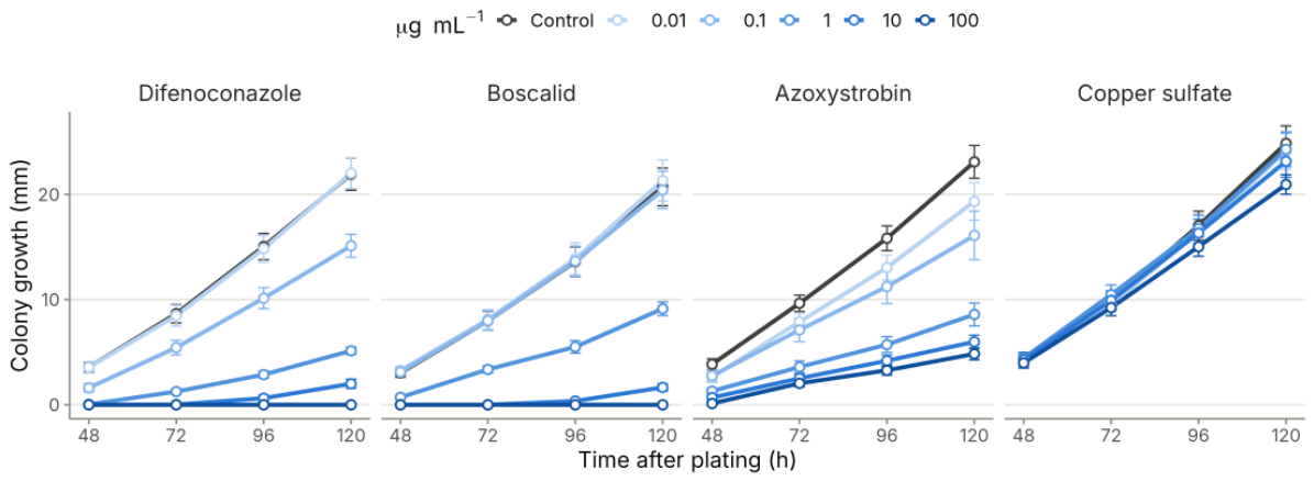
Figure 2.
Relative area under the mycelial growth curve (AUMGC, % of the control of the same isolate) of 23 M. roreri isolates at each fungicide concentration. Bars are means and grey points individual isolates. Within each panel, bars with different letters differ significantly (randomized complete block ANOVA with isolates as blocks, Tukey’s HSD, α = 0.05).
Figure 2.
Relative area under the mycelial growth curve (AUMGC, % of the control of the same isolate) of 23 M. roreri isolates at each fungicide concentration. Bars are means and grey points individual isolates. Within each panel, bars with different letters differ significantly (randomized complete block ANOVA with isolates as blocks, Tukey’s HSD, α = 0.05).
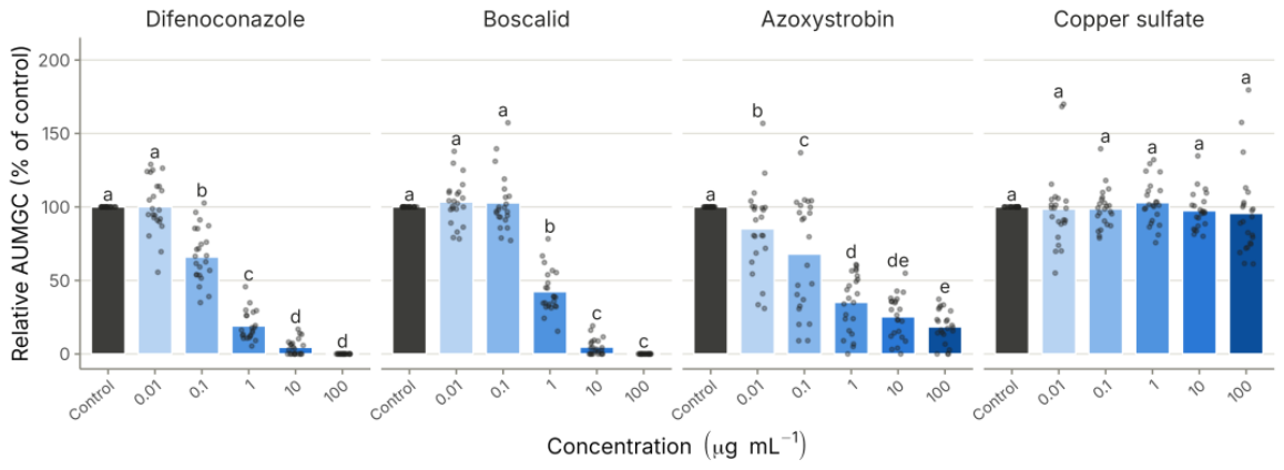
Figure 3.
EC50 of difenoconazole, boscalid and azoxystrobin for 23 M. roreri isolates, ordered by value. Symbols are point estimates and horizontal lines 95% bootstrap percentile intervals (300 resamples of plates within concentrations). Symbol shape indicates canton; for azoxystrobin, open symbols mark the less sensitive phenotype. The dotted line is the geometric mean of the estimates, the dashed line marks the category limit at 5 µg mL−1, and the shaded area lies below the lowest concentration tested (0.01 µg mL−1). Copper sulfate is not shown because all isolates had EC50 > 100 µg mL−1.
Figure 3.
EC50 of difenoconazole, boscalid and azoxystrobin for 23 M. roreri isolates, ordered by value. Symbols are point estimates and horizontal lines 95% bootstrap percentile intervals (300 resamples of plates within concentrations). Symbol shape indicates canton; for azoxystrobin, open symbols mark the less sensitive phenotype. The dotted line is the geometric mean of the estimates, the dashed line marks the category limit at 5 µg mL−1, and the shaded area lies below the lowest concentration tested (0.01 µg mL−1). Copper sulfate is not shown because all isolates had EC50 > 100 µg mL−1.
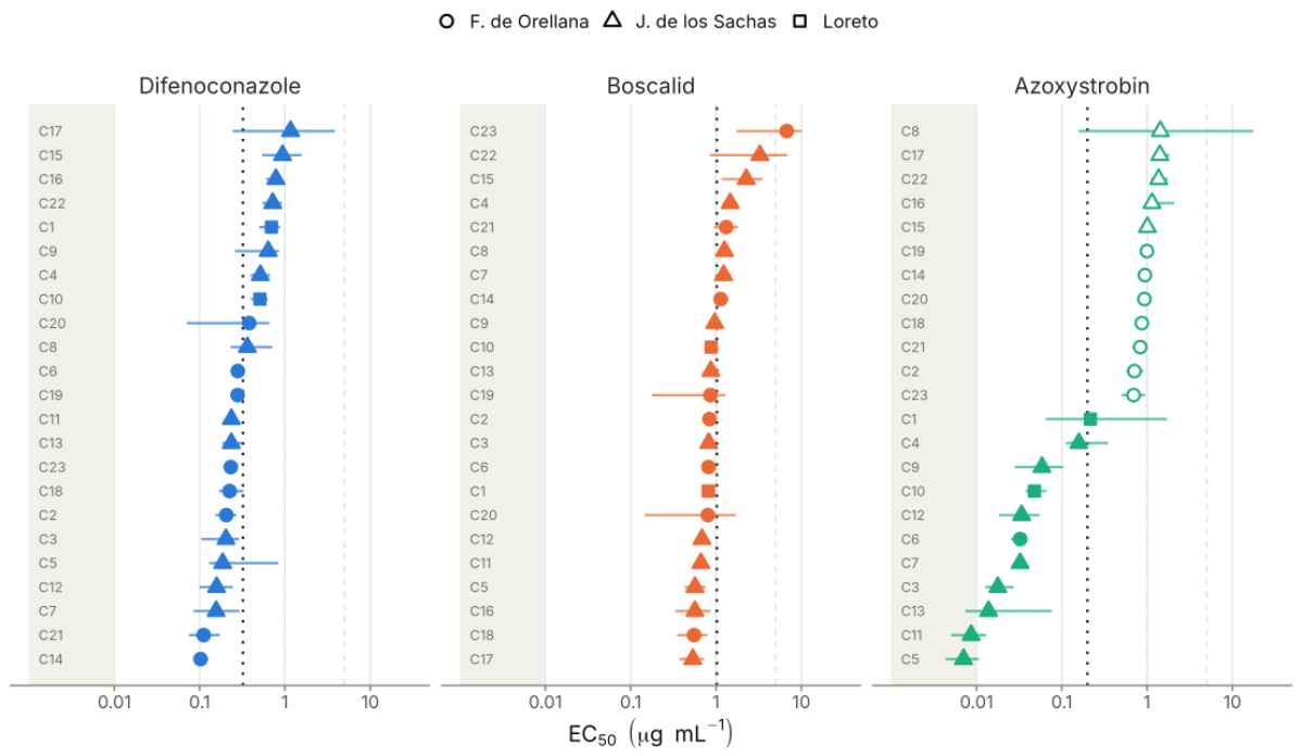
Figure 4.
Two azoxystrobin phenotypes among 23 M. roreri isolates. (A) Distribution of EC50 values on a logarithmic scale, coloured by the phenotype assigned by the two-component mixture model. (B) Inhibition of the mycelial growth rate (MGR) relative to the control. Thin lines are individual isolates and thick lines group means ± standard error; the dashed line marks 50% inhibition.
Figure 4.
Two azoxystrobin phenotypes among 23 M. roreri isolates. (A) Distribution of EC50 values on a logarithmic scale, coloured by the phenotype assigned by the two-component mixture model. (B) Inhibition of the mycelial growth rate (MGR) relative to the control. Thin lines are individual isolates and thick lines group means ± standard error; the dashed line marks 50% inhibition.
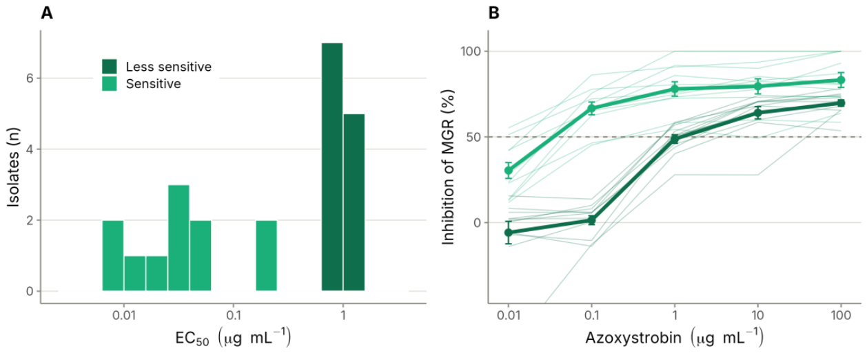
Figure 5.
Ward clustering of 23 M. roreri isolates by the standardized log10 EC50 of difenoconazole (Difeno.), boscalid and azoxystrobin (Azoxy.). Branch colours identify the five groups (blue, G1; orange, G2; green, G3; purple, G4; pink, G5). Cell colours are z-scores, and the numbers in the cells are EC50 values (µg mL−1). The copper column (Cu†) shows percentage inhibition at 100 µg mL−1 and was not used for clustering. Side bars indicate canton (Loc.), cacao genotype (Gen.) and farm.
Figure 5.
Ward clustering of 23 M. roreri isolates by the standardized log10 EC50 of difenoconazole (Difeno.), boscalid and azoxystrobin (Azoxy.). Branch colours identify the five groups (blue, G1; orange, G2; green, G3; purple, G4; pink, G5). Cell colours are z-scores, and the numbers in the cells are EC50 values (µg mL−1). The copper column (Cu†) shows percentage inhibition at 100 µg mL−1 and was not used for clustering. Side bars indicate canton (Loc.), cacao genotype (Gen.) and farm.
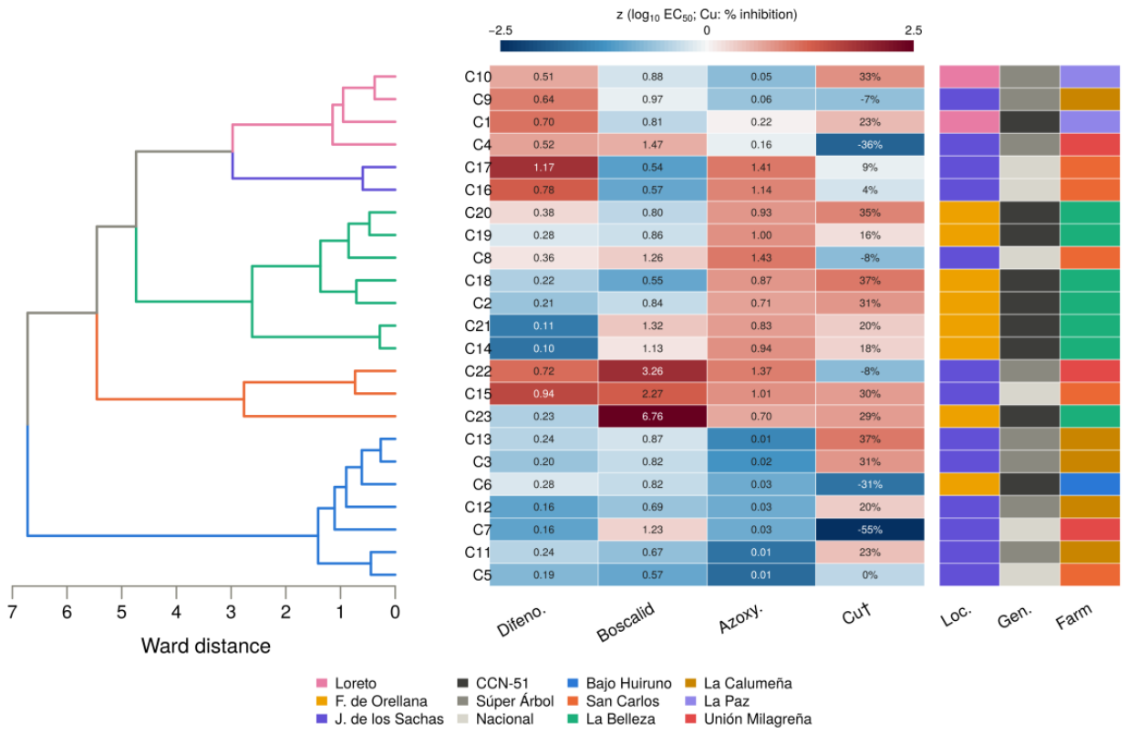
Figure 6.
Principal component analysis of the relative AUMGC of 23 M. roreri isolates at 0.1, 1 and 10 µg mL−1 of difenoconazole, boscalid, azoxystrobin and copper sulfate (12 standardized variables). (A) Isolate scores on PC1 and PC2. Colour indicates farm and symbol shape the azoxystrobin phenotype (circles, sensitive; triangles, less sensitive). Ellipses enclose 68% of a bivariate normal distribution fitted to each phenotype (solid, sensitive; dashed, less sensitive). (B) Correlation circle. Arrows show the correlation of each variable with PC1 and PC2, coloured by fungicide and labelled with the concentration (µg mL−1).
Figure 6.
Principal component analysis of the relative AUMGC of 23 M. roreri isolates at 0.1, 1 and 10 µg mL−1 of difenoconazole, boscalid, azoxystrobin and copper sulfate (12 standardized variables). (A) Isolate scores on PC1 and PC2. Colour indicates farm and symbol shape the azoxystrobin phenotype (circles, sensitive; triangles, less sensitive). Ellipses enclose 68% of a bivariate normal distribution fitted to each phenotype (solid, sensitive; dashed, less sensitive). (B) Correlation circle. Arrows show the correlation of each variable with PC1 and PC2, coloured by fungicide and labelled with the concentration (µg mL−1).
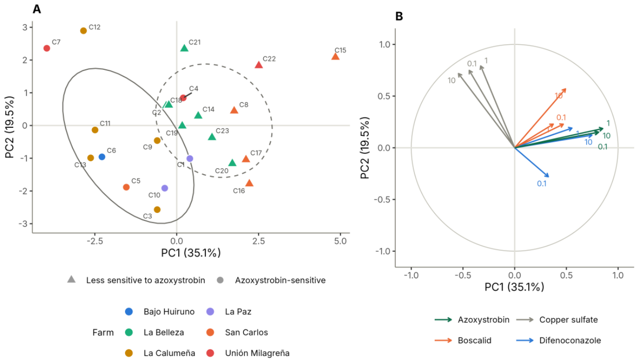
Figure 7.
Expected number of isolates per EC50 category among 300 simulated M. roreri isolates, by parametric Monte Carlo (M1, blue) and cluster smoothed bootstrap (M2, orange). Bars are means and whiskers 95% prediction intervals over 10,000 replicates. Simulated isolates are model predictions, not observations.
Figure 7.
Expected number of isolates per EC50 category among 300 simulated M. roreri isolates, by parametric Monte Carlo (M1, blue) and cluster smoothed bootstrap (M2, orange). Bars are means and whiskers 95% prediction intervals over 10,000 replicates. Simulated isolates are model predictions, not observations.
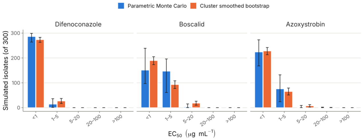
Figure 8.
(A) Fold half-width of the 95% interval of the estimated P95 of EC50 as a function of the number of isolates (3000 simulated samples per size, single log-normal distribution). Dotted lines mark the present collection (n = 23) and the collection enlarged by 300 isolates (n = 323). (B) Power of a two-sided t-test on log10 EC50 (α = 0.05) to detect an increase in the median EC50 of azoxystrobin, for four combinations of baseline and later sample sizes (23 vs. 23, 23 vs. 300, 323 vs. 100 and 323 vs. 50 isolates). The dashed line marks a power of 0.8.
Figure 8.
(A) Fold half-width of the 95% interval of the estimated P95 of EC50 as a function of the number of isolates (3000 simulated samples per size, single log-normal distribution). Dotted lines mark the present collection (n = 23) and the collection enlarged by 300 isolates (n = 323). (B) Power of a two-sided t-test on log10 EC50 (α = 0.05) to detect an increase in the median EC50 of azoxystrobin, for four combinations of baseline and later sample sizes (23 vs. 23, 23 vs. 300, 323 vs. 100 and 323 vs. 50 isolates). The dashed line marks a power of 0.8.
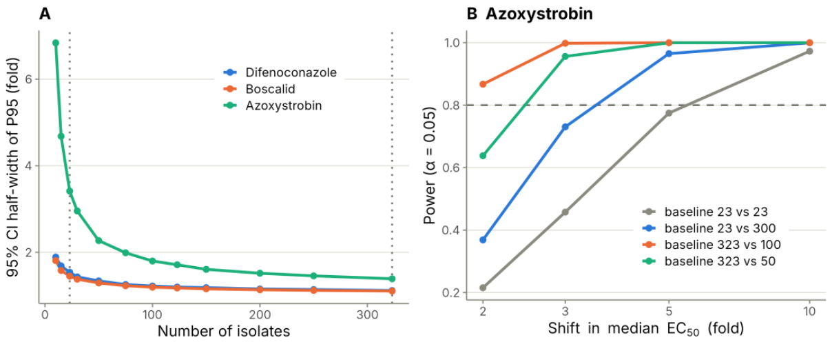

Table 1.
Origin of the 23 Moniliophthora roreri isolates (Orellana Province, Ecuador). Isolates whose field codes share a sample prefix (e.g., O-FO-03) came from the same field sample.
Table 1.
Origin of the 23 Moniliophthora roreri isolates (Orellana Province, Ecuador). Isolates whose field codes share a sample prefix (e.g., O-FO-03) came from the same field sample.
| Isolate | Field code | Canton | Parish | Farm | Cacao genotype | Sampling date |
|---|---|---|---|---|---|---|
| C1 | OL-P-07-A1 | Loreto | Puerto Murialdo | La Paz | CCN51 | 18 Oct 2021 |
| C2 | O-FO-05-A3 | F. de Orellana | La Belleza | La Belleza | CCN51 | 17 Aug 2021 |
| C3 | OS-LS-03-A1 | J. de los Sachas | Lago San Pedro | La Calumeña | Súper Árbol | 16 Jun 2021 |
| C4 | OS-UM-03-A1 | J. de los Sachas | Unión Milagreña | Unión Milagreña | Súper Árbol | 16 Jun 2021 |
| C5 | JS-SC-A1 | J. de los Sachas | San Carlos | San Carlos | Nacional | Oct 2021 |
| C6 | OL-09-A1 | F. de Orellanaa | Puerto Murialdo | Bajo Huiruno | CCN51 | 18 Jan 2022 |
| C7 | OS-UM-09-A1 | J. de los Sachas | Unión Milagreña | Unión Milagreña | Nacional | 21 Jan 2022 |
| C8 | OS-SC-03-A1 | J. de los Sachas | San Carlos | San Carlos | Nacional | 18 Jun 2021 |
| C9 | OS-LS-05-A3 | J. de los Sachas | Lago San Pedro | La Calumeña | Súper Árbol | 20 Aug 2021 |
| C10 | OL-03-A1 | Loreto | Puerto Murialdo | La Paz | Súper Árbol | 16 Jun 2021 |
| C11 | OS-LS-09-A3 | J. de los Sachas | Lago San Pedro | La Calumeña | Súper Árbol | 21 Jan 2022 |
| C12 | OS-LS-05-A2 | J. de los Sachas | Lago San Pedro | La Calumeña | Súper Árbol | 20 Aug 2021 |
| C13 | OS-LS-09-A1 | J. de los Sachas | Lago San Pedro | La Calumeña | Súper Árbol | 21 Jan 2022 |
| C14 | O-FO-09-A2 | F. de Orellana | La Belleza | La Belleza | CCN51 | 18 Jan 2022 |
| C15 | OS-SC-03-A2 | J. de los Sachas | San Carlos | San Carlos | Nacional | 18 Jun 2021 |
| C16 | OS-SC-05-A1 | J. de los Sachas | San Carlos | San Carlos | Nacional | 20 Aug 2021 |
| C17 | OS-SC-09 | J. de los Sachas | San Carlos | San Carlos | Nacional | 21 Jan 2022 |
| C18 | O-FO-03-A1 | F. de Orellana | La Belleza | La Belleza | CCN51 | 16 Jun 2021 |
| C19 | O-FO-05-A1 | F. de Orellana | La Belleza | La Belleza | CCN51 | 17 Aug 2021 |
| C20 | O-FO-03-A2 | F. de Orellana | La Belleza | La Belleza | CCN51 | 16 Jun 2021 |
| C21 | O-FO-09-A1 | F. de Orellana | La Belleza | La Belleza | CCN51 | 18 Jan 2022 |
| C22 | OS-UM-03-A2 | J. de los Sachas | Unión Milagreña | Unión Milagreña | Súper Árbol | 16 Jun 2021 |
| C23 | O-FO-MF-05 | F. de Orellana | La Belleza | La Belleza | CCN51 | 6 May 2022 |
F. de Orellana, Francisco de Orellana; J. de los Sachas, Joya de los Sachas. Totals: Joya de los Sachas 13, Francisco de Orellana 8 and Loreto 2 isolates; CCN51 9, Súper Árbol 8 and Nacional 6. Same-sample pairs: C2/C19, C4/C22, C8/C15, C9/C12, C11/C13, C14/C21 and C18/C20. a Canton as given in the collection record and the laboratory data sheet; the community of Bajo Huiruno lies in Loreto according to field records and ref. [9].
Table 2.
Fungicides evaluated, their FRAC classification [15] and the products used.
Table 2.
Fungicides evaluated, their FRAC classification [15] and the products used.
| Active ingredient | Chemical group | FRAC code (target site) | Target | Resistance risk | Product (manufacturer); a.i. content, formulation |
|---|---|---|---|---|---|
| Azoxystrobin | Methoxy-acrylate (QoI) | 11 (C3) | Cytochrome bc1, Qo site (complex III) | High | Amistar® 50 WG (Syngenta); 500 g kg−1, WG |
| Boscalid | Pyridine-carboxamide (SDHI) | 7 (C2) | Succinate dehydrogenase (complex II) | Medium to high | Cantus® (BASF); 500 g kg−1, WG |
| Difenoconazole | Triazole (DMI) | 3 (G1) | Sterol C14-demethylase (CYP51) | Medium | Score® 250 EC (Syngenta); 250 g L−1, EC |
| Copper sulfate | Inorganic copper | M01 | Multisite contact activity | Low | Phyton® 27 (Phyton Corp.); CuSO4·5H2O 240 g L−1, SL |
QoI, quinone outside inhibitor; SDHI, succinate dehydrogenase inhibitor; DMI, demethylation inhibitor; WG, water-dispersible granules; EC, emulsifiable concentrate; SL, soluble concentrate. Resistance risk as rated by FRAC for the group. Contents are given per kg or L of product; Phyton® 27 contains 240 g L−1 of the pentahydrate salt, equivalent to about 61 g L−1 of metallic copper.
Table 3.
EC50 (µg mL−1) of difenoconazole, boscalid, azoxystrobin and copper sulfate for 23 Moniliophthora roreri isolates.
Table 3.
EC50 (µg mL−1) of difenoconazole, boscalid, azoxystrobin and copper sulfate for 23 Moniliophthora roreri isolates.
| Fungicide | Range | GM [95% CI] | GSD | P95 [95% CI] | P99 [95% CI] | HS/S/MS/LS/VLS |
|---|---|---|---|---|---|---|
| Difenoconazole | 0.103–1.17 | 0.323 [0.242–0.438] | 1.96 | 0.98 [0.62–1.36] | 1.54 [0.89–2.29] | 22/1/0/0/0 |
| Boscalid | 0.535–6.76 | 1.02 [0.79–1.37] | 1.80 | 2.70 [1.26–4.99] | 4.04 [1.51–8.90] | 15/7/1/0/0 |
| without C20, C22, C23 a | 0.535–2.27 | 0.89 | — | — | — | 14/6/0/0/0 |
| Azoxystrobin, all b | <0.01–1.43 | 0.185 [0.062–0.441] | 7.15 | 4.71 [1.77–8.13] | 18.0 [6.0–37.4] | 18/5/0/0/0 |
| sensitive (n = 11) | <0.01–0.217 c | 0.035 | — | — | — | 11/0/0/0/0 |
| less sensitive (n = 12) | 0.695–1.43 | 1.00 | — | — | — | 7/5/0/0/0 |
| Copper sulfate | >100 (all) | — | — | — | — | 0/0/0/0/23 |
GM, geometric mean (median of the fitted log-normal distribution); GSD, geometric standard deviation; P95 and P99, 95th and 99th percentiles. CIs from a cluster bootstrap over the 16 field samples (1000 replicates). HS, highly sensitive (<1 µg mL−1); S, sensitive (1–5); MS, moderately sensitive (>5–20); LS, low sensitivity (>20–100); VLS, very low sensitivity (>100); values are numbers of isolates. a Isolates with low-vigour control plates (Section 3.2). b Single log-normal fit, inadequate for a bimodal distribution (Section 3.3); the fitted P95 and P99 lie above the highest observed value. c Includes two isolates with model estimates below the lowest concentration tested (0.0071 and 0.0087 µg mL−1). Per-isolate values with bootstrap and delta-method confidence intervals are given in Table S1.
Table 4.
Expected number of isolates in each sensitivity category, median and P95 among 300 simulated Moniliophthora roreri isolates over 10,000 replicates. Counts are means and the median and P95 are medians across replicates, each with its 95% prediction interval. The simulated isolates are model predictions, not observations.
Table 4.
Expected number of isolates in each sensitivity category, median and P95 among 300 simulated Moniliophthora roreri isolates over 10,000 replicates. Counts are means and the median and P95 are medians across replicates, each with its 95% prediction interval. The simulated isolates are model predictions, not observations.
| Fungicide | Method | HS (<1) | S (1–5) | MS (>5–20) | Median (µg mL−1) | P95 (µg mL−1) | Less sensitive (of 300) |
|---|---|---|---|---|---|---|---|
| Difenoconazole | M1 | 286.1 [264–299] | 13.8 [1–36] | ≈0 | 0.32 [0.24–0.44] | 0.94 [0.60–1.41] | — |
| M2 | 273.5 [263–283] | 26.5 [17–37] | ≈0 | 0.31 [0.27–0.35] | 1.18 [1.03–1.35] | — | |
| Boscalid | M1 | 150.9 [97–239] | 146.6 [61–196] | 2.5 [0–15] | 1.02 [0.79–1.38] | 2.60 [1.25–5.01] | — |
| M2 | 189.3 [173–205] | 92.8 [77–108] | 17.9 [10–26] | 0.86 [0.82–0.92] | 5.66 [3.22–6.80] | — | |
| Azoxystrobin | M1 | 223.9 [168–273] | 75.4 [24–132] | 0.6 [0–9] | 0.63 [0.04–0.94] | 1.37 [1.08–3.69] | 158.9 [85–227] (53%) |
| M2 | 228.0 [213–242] | 64.9 [51–79] | 7.0 [2–12] | 0.21 [0.12–0.33] | 3.35 [2.56–4.42] | 136.0 [119–153] (45%) |
M1, parametric Monte Carlo (log-normal distribution for difenoconazole and boscalid; two-component mixture for azoxystrobin; parameters drawn from cluster-bootstrap estimates); M2, cluster smoothed bootstrap (resampling of field samples and isolates with Gaussian kernel noise). HS, highly sensitive; S, sensitive; MS, moderately sensitive (EC50 classes in µg mL−1). Isolates with EC50 > 20 µg mL−1 were practically absent (mean ≤0.16 per 300 in every scenario). Less sensitive, number of simulated azoxystrobin isolates with EC50 ≥ 0.3 µg mL−1, with the percentage of 300 in parentheses. Copper sulfate was not simulated because no EC50 value lay within the tested range.
Disclaimer/Publisher’s Note: The statements, opinions and data contained in all publications are solely those of the individual author(s) and contributor(s) and not of MDPI and/or the editor(s). MDPI and/or the editor(s) disclaim responsibility for any injury to people or property resulting from any ideas, methods, instructions or products referred to in the content. |
© 2026 by the authors. Licensee MDPI, Basel, Switzerland. This article is an open access article distributed under the terms and conditions of the Creative Commons Attribution (CC BY) license (http://creativecommons.org/licenses/by/4.0/).
Copyright: This open access article is published under a Creative Commons CC BY 4.0 license, which permit the free download, distribution, and reuse, provided that the author and preprint are cited in any reuse.