
Submitted:
16 November 2026
Posted:
17 November 2026
You are already at the latest version
Abstract
Computational studies of phase transitions and superconducting materials depend on how microscopic configurations, spatial heterogeneity, and material descriptors are represented. This study combines Monte Carlo sampling, symmetry-aware classification, numerical BCS calculations, geometric connectivity analysis, and supervised materials prediction to examine the consequences of those choices. In a disordered 2D Ising model, classifiers based on spin-flip-invariant features achieved 100% balanced accuracy in the tested temperature extremes across all three disorder levels, with no disagreement between spin-reversed configurations. In prescribed BCS scenarios, widening the coupling distribution at fixed mean coupling increased the mean local pairing temperature by 44.2%. Rearranging an unchanged distribution of couplings altered geometric spanning thresholds, demonstrating the additional importance of spatial organization. For critical-temperature prediction, mean root-mean-square error increased from 9.85 K under random row splitting to 13.70 K when entire chemical systems were held out. Retrospective screening of the highest-ranked 10% of held-out compositions achieved 86.4% precision for the defined high-temperature target. In supplementary nanoparticle data, a single descriptor achieved 96.1% balanced accuracy compared with 99.2% using all features, highlighting uncertainty about the physical meaning of the recorded labels. These results establish the value of symmetry-aware representations and explicit validation of heterogeneity, geometry, and data splits.
Keywords:
materials
; superconductors
; computational physics
; applied physics
; neural networks
1. Introduction
Many quantum many body systems contain very large amounts of interacting particles forming configurations that cannot generally be solved analytically. These condensed matter systems demonstrate complex collective behavior at different scales that are difficult and unintuitive to predict from their microscopic properties and interactions. In particular, superconductors go through phase transitions where the material produces 0 electrical resistance and magnetic-field expulsion under a critical temperature. At the nanoscale, disorder and structure can modify these properties in certain ways. These nonlinear, many-body, high dimensional systems generally require numerical methods, and computational solutions can be impractical or still open to much optimization.
One important problem is identifying phase transitions–where a system such as a material changes from macroscopic one state of matter to another–which can be predicted based on variables like temperature and interaction strength changes. Phase transitions are particularly relevant for studying superconducting nanomaterials since discerning the critical point where the material gains its superconducting properties is an important area of interest and utility. These transitions are often described using an order parameter, a specific quantity that is used to distinguish different phases. Monte-Carlo methods can be used to do this by repeatedly sampling variations of accessible microscopic conformations and then machine learning (ML) methods can be used to quickly and accurately analyze the results for patterns and parameters.
2. Literature Overview
2.1. Monte Carlo Sampling and Machine Learning for Phase-Transition Detection
2.1.1. Generating Physically Meaningful Configurations
In the relevant many-body systems, phase transitions are commonly identified through changes in macroscopic observables such as magnetization, energy, or an order parameter. Monte Carlo methods address this challenge by repeatedly sampling configurations from a system’s probability distribution and using those samples to estimate equilibrium properties. The resulting configurations can then be analyzed using machine-learning methods.
The aforementioned creates a useful connection between numerical physics and machine learning: Monte Carlo methods generate physically motivated data, while machine-learning models identify patterns within that data. In this framework, the model is not replacing the underlying physical simulation. Instead, it provides a method for extracting features that may be difficult to detect using conventional observables alone.
2.1.2. Convolutional Neural Networks Applied to Quantum Monte Carlo Data
Dong et al. demonstrate the aforementioned approach by combining quantum Monte Carlo simulations with a convolutional neural network (CNN), a type of deep learning algorithm designed to process grid-like data, such as images and graphs, by learning its spatial features.
Their quantum Monte Carlo configurations are represented in a -dimensional space, where the additional dimension corresponds to imaginary time. Since the complete configuration space can become too large to use directly as a neural-network input, the authors compress the configurations while attempting to preserve their physically relevant information. The compressed configurations are then provided to a CNN, which learns spatial and temporal patterns associated with different phases. The study shows that this approach can detect both continuous and discontinuous quantum phase transitions. It also demonstrates that an intermediate phase that was not explicitly included during training could still be identified by the network, suggesting CNNs can recognize phase-dependent patterns in microscopic configurations without requiring every possible phase to be manually labeled (Dong et al., 2019).
One significant implication here is that the CNN does not need to be given the exact physical order parameter as an input; instead it learns features from the configuration data. However, the output of a CNN should still be compared with known physical quantities because high classification accuracy alone does not prove that the network has learned the underlying physics. The network may also just be responding to finite-size effects, sampling artifacts, or correlations specific to the training data.
2.1.3. Unsupervised Learning of Phase Transitions
Wetzel studies a related problem using unsupervised learning: Rather than training a model with preassigned phase labels, principal component analysis (PCA) and variational autoencoders (VAEs) are applied to Monte Carlo configurations from the 2D Ising model and the 3D XY model. In this study, PCA identifies directions of greatest variance in the configuration data, while the VAE learns a lower-dimensional representation through nonlinear encoding and reconstruction.
In both cases, the learned latent variables correspond closely to known order parameters. The configurations also form distinguishable groups in the learned representation, allowing the phases to be identified without explicitly providing the model with phase labels and/or the correct order parameter.
This result is particularly relevant since the 2D Ising model provides a controlled test case in which the expected phase behavior is already known. PCA, t-SNE, or related dimensionality-reduction methods can then be evaluated by comparing their patterns with magnetization and the known critical temperature. These methods are particularly useful specifically for visualizing structure in the noisy, high dimensional data (Wetzel, 2017).
2.1.4. Interpreting Learned Features
Neural networks like CNNs are effective at identifying patterns but their internal representations can be difficult to interpret physically. Ju et al. examine this issue by studying how CNNs approximate quantum spin systems when combined with variational Monte Carlo methods. Their analysis connects the network’s learned representation to physical symmetries, local spin motifs, and the structure of the variational wave function.
The authors show that a shallow CNN can represent important correlations using a number of parameters that grows much more slowly than the full dimension of the many-body Hilbert space. They further relate the CNN representation to statistical and physical models based on local motif frequencies and correlations. This suggests that the success of a CNN is not mysterious or a black box: the network can exploit locality, repeated patterns, and symmetry within the spin configuration (Ju et al., 2025).
These studies show several complementary uses of ML. Supervised CNNs can classify or detect phases, unsupervised methods can identify latent structure without phase labels, and interpretability studies can investigate which physical features are responsible for the model’s predictions.
2.2. Reduced Representations and Materials Design
2.2.1. Reducing the Search Space of Complex Systems
A primary challenge when studying condensed matter systems with many interacting microscopic particles is computational cost and complexity. As previously touched upon, many-body quantum systems can contain exponentially large Hilbert spaces and materials exhibit disordered and nonlinear complexities that can’t be reduced to an analytical description or solution.
Conventional numerical methods like Monte Carlo or exact diagonalization can be utilized when conducting research on these systems. However, performing these tasks becomes increasingly computationally expensive as system size and dimensionality increase. ML provides an alternative approach, with being able to identify patterns and parameters in computational simulation data.
ML results can then be used to create a lower-dimensional representation of the system that still retains relevant physical information. Dimensionality reduction is particularly useful to reduce computational costs, and not every microscopic degree of freedom contributes equally significantly to the properties of the material. Therefore, we can integrate some of those degrees of freedom out of the system without losing any information that is too important, an approach that is also shared with some methods like mean-field continuum models.
These statistical and ML methods can identify correlations among variables which allows features of the system to be represented with fewer parameters, reducing the computational cost of classification, optimization, and prediction while still creating a useful representation of the material. They complement traditional numerical methods and simulations by extracting meaningful information out of complex high-dimensional data.
2.2.2. Graph Representations of Physical Neural Networks
Graph theory is a branch of mathematics that studies networks made up of points connected by lines, which model the relationships between the components of a system.
Obernolte et al. (2026) use a graph-theoretic representation to demonstrate the optimization of a physical system through these connections rather than simulating each individual possible configuration. In particular, their research was focused on investigating physical neural networks formed by interconnecting nanoscale optical waveguides that exhibited strong lasing modes and nonlinear dynamics in their interactions. Through these dynamics the networks can be used to perform image-processing tasks, but identifying effective ways to structure the networks involves searching through an extremely large amount of possible configurations.
To approach this problem, the authors of this paper constructed graph representations where nodes and edges described the topology of the physical network. Graph-theoretic metrics are then used to measure and predict aspects of lasing behavior and associated classification performance and then an evolutionary algorithm is also utilized. The researchers reported approximately a 3,000-fold reduction in design evaluation cost compared with repeated physical simulations. These results demonstrate that structural information can serve as an efficient approximation of complicated nonlinear behavior.
The underlying approach to this paper demonstrates that structural relationships among components can be represented mathematically and analyzed without explicit calculations of every microscopic interaction. Similar strategies to the one used there could be applied to materials which have electronic or transport properties that depend strongly on geometry, connectivity, and disorder.
2.2.3. Machine Learning for Designing Materials
ML and computational numerical methods are also important tools for materials science specifically, since it is an area where predicting physical properties often requires computationally expensive simulations or experimental measurements.
One example is a Cao et al. (2024), in which the authors review three applications of machine learning to the design of porous membranes, including polymeric and 2D materials: predicting material properties, using explainable machine learning to identify relationships between structure and performance, and optimizing new material designs through computational screening. ML models can approximate relationships between structural descriptors and material performance, potentially reducing the number of simulations required to evaluate candidate structures. Explainable models can also assist in identifying what physical properties contribute most strongly to a prediction.
Another example is Wines et al. (2023), where the researchers demonstrate a high-throughput computational approach for discovering two-dimensional superconductors using density functional theory and electron-phonon coupling calculations. After screening more than 1,000 two-dimensional materials, the researchers perform detailed superconductivity calculations for 165 candidates and identify 34 dynamically stable structures with predicted critical temperatures above 5 K. This study illustrates the computational demands of searching large materials databases and provides a potential segue into ML applications, since combining such datasets with trained predictive models could help prioritize promising candidates for more detailed calculations.
2.2.4. BCS Theory and Continuum Models
A method of averaging out interactions across a large system is using a mean-field continuum model. This allows us to approximate the general, macroscopic state of a system. Here, we create a basic simulation for a superconducting phase transition based on numerically solving the BCS (Bardeen-Cooper-Schrieffer) self-consistency equation, the fundamental mean-field equation in BCS theory that determines the superconducting energy gap parameter delta, at many different temperatures:
Here, represents the dimensionless pairing interaction strength, is the energy cutoff, and represents electron energy relative to the Fermi level. The calculation used units with Boltzmann’s constant equal to one, an energy cutoff of = 1, and a coupling strength of = 0.30.
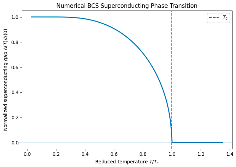
The superconducting gap acts as an order parameter where below , , while at and above it becomes equal to 0. For the parameters in the script, the numerical result also gives the expected weak coupling BCS value of critical temperature (model units), low-temperature gap , and .
Bardeen, Cooper, and Schrieffer (1957) established their microscopic theory of superconductivity when an effective attractive interaction between electrons produces Cooper pairs and an associated superconducting energy gap. Within the weak-coupling approximation, the critical temperature depends exponentially on the pairing interaction strength, making it particularly sensitive to changes in the model’s coupling parameter.
More recently, Dodaro and Kivelson (2018) conducted an investigation of spatially inhomogeneous solutions of the BCS gap and demonstrated that disorder can enhance the mean-field pairing instability through rare regions with favorable local properties. However, they also found that local enhancement of pairing does not necessarily translate to or imply an increase in the experimentally observed superconducting transition temperature. This is because fluctuations and interactions between different superconducting regions can influence global coherence.
Dubi, Meir, and Avishai (2007) find that disorder can produce spatially separated superconducting “islands,” areas where the local superconducting order parameter still remains significant as correlations between different regions weaken. Subsequent calculations using the Bogoliubov-de Gennes equations also illustrated the formation and evolution of these islands under applied magnetic fields (Dubi et al., 2008).
Additionally, experimental evidence for spatial inhomogeneity was presented by Sacépé et al. (2008).
2.3. Symmetry as a Physical Feature and Computational Advantage
Symmetry is a fundamental mathematical principle in condensed matter physics because it describes transformations that leave important properties of a system unchanged. Examples include translational symmetry, rotational symmetry, parity, and time-reversal symmetry. It often introduces mathematical tricks that make it easier to solve problems with the given parameters of a system, whether that’s analytically or numerically.
In computational physics and nanoscience, symmetries help determine which physical states are possible, how phases can be classified, and how materials respond to external conditions; this is useful for numerical simulations as they can also reduce computational complexity by identifying equivalent configurations or restricting calculations to physically relevant states.
2.3.1. Symmetry in Superconducting Systems
Tsai et al. (2026) investigate the breaking and restoration of parity-time symmetry in superconducting Josephson junctions. Their experimental system consists of NbTi//NbTi junctions in which superconducting interference patterns depend on the orientation of an applied magnetic field. When the in-plane field is aligned parallel to the current, the researchers observe pronounced asymmetry in the interference pattern, and rotating the field perpendicular to the current restores a combined parity-time-symmetric response under the conditions studied.
The authors associate this behavior with the interaction between disorder-induced potential variations and magnetic-flux structures produced near the superconducting electrodes. Their results demonstrate that the symmetry of a nanoscale superconducting device can be manipulated through external field geometry. Numerical models must account for how symmetry, disorder, and external conditions influence experimentally observable properties, which is a highly relevant principle to keep in mind for computational nanomaterials and condensed matter research.
2.3.2. Symmetries and Disorder Averaging
Disorder creates additional difficulties in numerical simulations since random interactions or structural variations often break the symmetries that would simplify a physical model. Simulating individual disorder realizations can be computationally demanding, particularly when the final observable requires averaging over many possible configurations.
Erpelding et al. (2026) investigate how disorder averaging can produce effective symmetries in quantum dynamics by applying disorder averaging to dynamical evolution–rather than requiring separate simulations of every realization. For observables that depend linearly on the evolved quantum state over some period of time, the resulting averaged dynamics can possess symmetries that individual disorder realizations do not.
This approach is demonstrated using an Ising model with random all-to-all interactions and an external transverse magnetic field. Although individual realizations lack permutation symmetry, the disorder-averaged dynamics become effectively permutation-invariant, which allows the system to be represented within a symmetric subspace whose size grows polynomially rather than exponentially with the number of spins.
The restored symmetry applies to the averaged dynamical description rather than necessarily to each microscopic realization, and numerical methods can exploit statistical properties of disorder to recover useful mathematical structure.
2.3.3. Symmetry-Preserving Neural-Network Quantum States
Symmetry is a classical trick for numerical methods but it can also be incorporated directly into ML architectures. Symmetry-preserving models encode the constraints of materials’ properties into their mathematical structure, effectively reducing the search space of the optimization problem while also helping to prevent physically inappropriate solutions.
Rende et al (2026) investigate this approach using a neural-network quantum state for the two-dimensional Hubbard model, a model which is commonly used to study strongly correlated electrons and unconventional superconductivity. Variational calculations of this model can favor particular broken-symmetry configurations depending on the chosen wave-function, initialization, and boundary conditions which can cause outputs that appear like results but are really just artifacts or noise from the numerical method.
To try and solve this, the authors introduce a Symmetry-Preserving Backflow Pairing ansatz that maintains translational symmetry by construction. Using systems containing up to 504 electrons on 24 24 lattices, they obtain low variational energies. As a result, they report evidence for d-wave superconducting order under selected Hubbard-model parameters.
This suggests incorporating known symmetries into neural-network wavefunctions can improve the reliability of numerical investigations of competing quantum phases.
2.3.4. Ising-Model Studies
The classical Ising model, a foundational framework in statistical physics, provides a starting point for investigating the relationship between numerical simulation, machine learning, and symmetry. It can be used as a controlled benchmark for investigating whether the computational and numerical methods we use can identify phase behavior and symmetry-related patterns, before those methods are extended to more complicated quantum systems.
The Ising model’s simplest form consists of spins that can take values of +1 or 1, with interactions that favor or oppose alignment between neighboring spins. The Hamiltonian of a nearest-neighbor ferromagnetic Ising model without an external magnetic field is , where J is the interaction strength and represents the spin at lattice site i.
The 2D Ising model undergoes a continuous phase transition between an ordered ferromagnetic phase at low temperatures and a disordered paramagnetic phase at higher temperatures. In the absence of an external field, the Hamiltonian remains unchanged when every spin is reversed. This global spin-flip symmetry, or symmetry, provides a demonstration of the relationship between symmetry and phase transitions.
The zero-field, nearest-neighbor Ising model on a clean square lattice has a known analytical solution; higher-dimensional cases are generally studied numerically. There are a variety of numerical methods that can be used to simulate these dimensions as well as examine configurations in any dimension under certain parameters. Monte Carlo simulations can be used to generate spin configurations across a range of temperatures that can be examined using observables (such as magnetization and energy) along with ML methods. Changes in spin correlations and magnetization near can be compared with changes in learned low-dimensional representations.
2.3.5. t-Distributed Stochastic Neighbor Embedding
t-Distributed Stochastic Neighbor Embedding (t-SNE) is a nonlinear dimensional reduction method developed by van der Maaten and Hinton (2008): it is designed to visualize high-dimensional datasets by mapping observations into a lower-dimensional space, typically of two dimensions, while attempting to preserve relationships between nearby points. The algorithm represents similarities between observations in probabilistic terms and then optimizes the low-dimensional representation to approximate these relationships.
3. Methods
3.1. Experimental Design
Based on the frameworks described in Section 1 and Section 2 of this paper, we performed a series of computational experiments to further investigate how numerics and ML can be used to detect and characterize phase transitions, disorder, and properties of superconducting materials. These experiments were designed with the intention to study the influence of physical symmetry on ML classification, how superconducting pairing relates to spatial connectivity, predicting critical temperatures of superconductors based on their material properties, and identifying potential biases and limitations in the datasets used.
We first use Monte Carlo configurations of the 2D Ising model to benchmark phase recognition under different degrees of disorder by training ML models on configurations from the system under a non-disordered control trial. We then evaluate the models on independently generated configurations with different disorder widths. Conventional and symmetry-aware representations were both examined to observe differences in how the results from the different methods vary when they are both used to study the same physical states.
Next, we examine spatial heterogeneity by simulating superconductivity by combining a local BCS approximation with a lattice connectivity model. This was done to discern temperature-dependent activation of specific regions from continuous pathway formations within the whole system. Supervised regressions were applied separately to data on superconducting materials to investigate the variation in critical temperature predictions under different validation strategies. We also supplement with an analysis of nanoparticles in order to assess potential correlations between numerical features and predefined classification labels.
3.2. Ising Model and Monte Carlo Sampling
The model consists of a 20 20 square lattice with periodic boundaries and spins = 1. Rightward and downward bonds are counted once in the zero-field Hamiltonian:
Independent uniform draws define each bond. The disorder width is w = 0, 0.35 or 0.75. The bonds remain positive and are fixed within a chain across all temperatures, preserving global spin-flip symmetry. Temperature is expressed in units of the mean bond energy divided by , with both set to one.
Configurations are sampled using checkerboard Metropolis updates with acceptance probability . The even lattice size permits alternating sublattice updates. The temperature grid is 1.55, 1.75, 1.95, 2.10, 2.20, 2.30, 2.40, 2.50, 2.60, 2.75, 2.90, 3.10 and 3.30. This grid brackets, but does not contain exactly, the clean infinite-lattice critical temperature .
Each temperature starts from a new random spin configuration. After 350 thermalization sweeps, 18 snapshots are collected, each after a further 18 sweeps. Four clean training chains produce 936 snapshots. Four additional clean test chains and four test chains at each nonzero disorder width produce 2,808 test snapshots. Independence refers to distinct chains and bond realizations; snapshots from the same chain can remain correlated. The original master seed is 20261020.
The magnetization , energy per spin, and the finite-size fluctuation proxy are calculated separately within each chain, then averaged across the four test realizations at each disorder width. Shaded bands show standard errors across those realizations. The proxy is useful for locating a broad finite-size response, but it is not a precise thermodynamic susceptibility or a bulk critical-temperature estimate.
3.3. Classification and Symmetry Controls
Training labels are assigned only to clean snapshots at T 1.95 and T 2.90, giving 432 labeled training snapshots before augmentation. Intermediate temperatures are excluded from label fitting. The corresponding test regions contain 432 snapshots per disorder width, or 1,296 in total. Each is evaluated together with its globally reversed counterpart. Temperature and disorder width are never classifier inputs.
Six models are compared: an unaugmented raw-spin linear model; the same raw-spin model with spin-flip augmentation; a linear model on sign-aligned spins; a linear model on ten pair-correlation features; a linear model using alone; and a nonlinear radial-basis-function support-vector machine on raw spins. Sign alignment multiplies a configuration by the sign of its total magnetization, using the first spin to resolve an exactly zero total. Correlation features average products at offsets one through five along both lattice axes.
Except for the explicitly unaugmented control, training examples include both s and s with the same class label. StandardScaler is fitted within each training pipeline. Logistic regression uses C = 1, balanced class weights, a maximum of 2,500 iterations and the fixed seed. The support-vector machine uses C = 2 and gamma = scale. No hyperparameter search is performed on the test set.
Balanced accuracy is the mean of the two class recalls, evaluated across original and reversed test configurations. Spin-flip disagreement is the fraction of pairs with different hard predictions. Zero disagreement alone is insufficient: a constant prediction is perfectly invariant and uninformative. The original implementation checks the invariance of the Hamiltonian, aligned features, correlation features and directly, and checks separation of clean training and test chains.
3.4. Dimensionality Reduction
For visualization, ten held-out snapshots are selected from each of the 39 disorder–temperature bins, giving 390 configurations. Raw spins and an invariant map of nearest-neighbor spin products are separately compressed to 30 principal components and embedded in two dimensions with t-SNE. The t-SNE settings are perplexity 30, PCA initialization, automatic learning rate and 900 iterations, using the original fixed seed. These transformations use the visualization subset; their coordinates are not used for supervised fitting or scoring.
Intermediate-temperature prediction curves and embeddings are exploratory. A classifier probability of 0.5 is not a physical critical-temperature measurement, and t-SNE distances or clusters do not establish a phase transition. The small lattice, four disorder realizations per test condition, coarse temperature grid and unquantified near-critical autocorrelation limit inference. The earlier simulation outputs are retained; the new database experiments do not constitute additional Ising Monte Carlo sampling.
3.5. Data Sources
Three supplied archives extend the controlled Ising example through complementary questions: how nonlinear BCS responses change under heterogeneity, how spatial arrangement affects connectivity, and how reliably composition descriptors support materials screening. The datasets are analyzed separately because they contain neither common sample identifiers nor a validated mapping between their physical variables.
The superconductivity archive matches the schema of the UCI dataset documented by Hamidieh (2018a, 2018b): 21,263 rows with 81 descriptors and a critical temperature in kelvin, accompanied by chemical formulas and elemental counts. Rowwise critical temperatures agree exactly across the two files. Normalizing elemental counts to atomic fractions and rounding to eight decimals gives 15,164 composition groups; grouping by the set of present elements gives 3,365 chemical systems. There are 2,422 composition groups with repeated records, including 2,375 with differing temperatures. These differences are retained rather than assumed to be measurement errors; synthesis conditions and structure are not available to resolve them. The second archive contains 1,200 rows with columns named lambda_0, mean_lambda, mean_t_c and direct_t_c. The lambda_0 values form an evenly spaced grid from 0.073 to 0.500, with mean 0.2865. The file supplies no unit definitions, uncertainty estimates or generation protocol. It is used as a parameter-grid benchmark, not as an experimentally measured distribution of material disorder. The three nanoparticle files are described separately in the nanoparticle subsections.
3.6. BCS Calculations
The homogeneous demonstration in Figure 1 uses adaptive quadrature and Brent root finding with = 0.30 and cutoff = 1. The temperature sweep contains 160 points from to . The plotted gap is normalized by the lowest-temperature value, used as an approximation to the zero-temperature gap.
The original BCS example is extended using the same isotropic mean-field gap equation (Bardeen et al., 1957), with and the cutoff energy set to one:
The critical temperature is obtained from the linearized equation at = 0 using Brent root finding in log T on [40, 2], with absolute and relative tolerances . The transformed integral uses ; above u = 25, its exponentially small correction is neglected and the remaining logarithmic tail is integrated analytically. At zero temperature, . For 0 < T < , the substitution gives a smooth integral evaluated using 96-point Gauss–Legendre quadrature, followed by Brent root finding for with tolerances . The gap is set to zero at and above .
The supplied direct_t_c values are compared with the calculated unit-cutoff values after fitting one multiplicative scale as their median ratio. This is a numerical consistency check, not independent experimental validation or proof of the original unit convention.
A deliberately chosen family of independent-domain scenarios preserves mean coupling while widening its distribution:
Each domain has its own local and gap. All 1,200 grid points are used for the mean local and the paired fraction . Mean-gap curves for w = 0, 0.5 and 1 use 121 equally weighted midpoint quantiles of the grid at 121 temperatures from zero to 0.18; the homogeneous case is solved once per temperature. Because the supplied grid is uniform, this is a prescribed uniform-disorder experiment whose range is anchored to the file. It does not estimate disorder in any specific material. The inputs mean_lambda and mean_t_c are retained for descriptive comparison, but their unreported averaging process is not reverse-engineered.
Numerical checks compare 96 and 192 point quadrature at four coupling strengths and T/ = 0.1, 0.9, 0.99 and 0.999. Domain averaging is checked at T = 0.01, , 0.08 and 0.13 using 61, 121 and 241 midpoint quantiles. Solver checks and domain-resolution differences are reported separately because they quantify different numerical errors.
3.7. Spatial Connectivity
The same coupling distribution is placed on square lattices of side length L = 24, 48 and 96. Each lattice contains the corresponding midpoint quantiles of the supplied lambda_0 grid. For every size, 120 independent standard-normal random fields are generated. Each field is either unsmoothed or Gaussian-smoothed with standard deviation = 2 or 5 lattice sites and reflecting boundaries. Sorting the field assigns the fixed sorted coupling list by rank, preserving exactly the same marginal distribution across the three arrangements. The same random field is reused across smoothing widths within a replicate.
A site is occupied when its local is at least the tested temperature. Open boundaries and four-neighbor connectivity define a left-to-right spanning path. Binary search over the ordered local temperatures identifies the largest threshold at which a path exists, ; the implementation verifies spanning at that threshold and failure at the next higher one. A smoothed Gaussian field is a specified construction of spatial correlation, not an inferred microstructure. is measured in lattice sites, not nanometers.
Spanning probability is the fraction of 120 realizations that span at a given temperature. Threshold summaries report medians and the central 95% range across realizations. These ranges characterize disorder variability, not a confidence interval for a thermodynamic critical point. The model contains no Josephson coupling, phase dynamics, phase stiffness, proximity effect or transport equation. therefore describes geometric connectivity only.
3.8. Materials Prediction and Retrospective Screening
The 81 descriptors in train.csv predict the recorded critical temperature. Elemental counts and formula strings are used only to define groups, not as additional predictors. The descriptor named thermal conductivity is not interpreted as an electron–phonon coupling constant. No material-specific BCS parameters are inferred from this database.
Three evaluation schemes are repeated for seeds 20261021 through 20261025: a random 80:20 row split; an 80:20 split of normalized composition groups; and an 80:20 split of chemical-system groups. GroupShuffleSplit selects 20% of distinct groups, so the resulting fraction of rows can differ from 20% (Scikit-learn developers, n.d.-a). Grouped evaluations enforce zero overlap between training and test groups. The random-row result is retained as an optimistic comparison. Differences among schemes combine changes in duplication exposure and chemical-domain difficulty and are not attributed solely to data leakage.
Fixed model settings are used throughout: a training-target-mean baseline; ridge regression with StandardScaler fitted on training data and = 10; and histogram gradient boosting with 180 iterations, learning rate 0.08, at most 31 leaves, at least 20 samples per leaf and L2 regularization 1. Early stopping is disabled, and the split seed is used as the model seed (Scikit-learn developers, n.d.-b). No test-set hyperparameter selection or post hoc tuning is performed. Predictions are not clipped.
Performance is summarized by row-weighted root-mean-square error (RMSE), mean absolute error and . A composition-balanced RMSE is also computed by first averaging squared errors within each held-out composition, then averaging across compositions and taking the square root. Repeated temperatures are retained in model fitting. The main reported error bars are standard deviations across the five split results; overlapping holdouts mean these are not independent cross-validation folds or confidence intervals.
Retrospective screening uses only the two grouped holdouts. Each test pool is collapsed to one candidate per normalized composition: its recorded temperature is the median of its test records, and its predicted score is the mean prediction. Candidates are ranked by predicted score. Budgets select the highest-scoring 1%, 5%, 10%, 20%, 50% or 100%, rounding the number selected upward. A hit has median recorded 77 K. Precision is hits divided by the number selected; recall is hits divided by all hits in the held-out pool. Enrichment is precision divided by pool prevalence. The random-screening baseline is the expectation under uniform candidate sampling.
The 77 K cutoff is a predefined screening threshold and is not a label for a microscopic phase configuration. The database contains known superconductors and does not test whether an unobserved material is superconducting (Hamidieh, 2018a). Consequently, this experiment measures prioritization within a historical database; it does not establish prospective discovery, synthesis feasibility, experimental cost savings or a new superconducting mechanism.
3.9. Nanoparticle Controls
The nanoparticle archive contains three incompatible tables. Data.xlsx.csv has 2,184 rows, seven numerical columns and a three-level C label. Dataset.csv has 2,186 rows, five numerical predictors and a continuous C target. Nanoparticles properties.csv has 2,187 rows, eight numerical columns and a five-level Classes label. Decimal commas are parsed explicitly, the last file uses semicolon delimiters, and entirely empty trailing columns are removed. No rows are joined across files, and no undocumented units or meanings are assigned to the abbreviated columns. For each table, five 75:25 train/test splits use the same seed list as the materials-prediction methods; classification splits are stratified. Fixed gradient-boosting settings match the materials-prediction methods. Full-feature models are compared with -only models, models omitting , and models trained on a permuted training target. Numerical noise tests add independent zero-mean Gaussian perturbations with standard deviations 0.05, 0.10 or 0.20 times each training-feature standard deviation, only at prediction time. This can move values outside their original range and is used simply as a software robustness test.
3.10. Computational Environment and Benchmarking
The BCS heterogeneity, connectivity, materials-prediction and nanoparticle experiments use Python 3.12.14, NumPy 2.3.5, SciPy 1.17.0, pandas 2.2.3, scikit-learn 1.8.0 and Matplotlib 3.10.8. The main seed is 20261021. Spatial seeds are , with . Numerical library threads are limited to two for fitting. The separate computational reproducibility package contains unchanged input archives, their SHA-256 fingerprints, the executed notebook, the simulation module, figures in three formats, numerical solver checks, all connectivity replicates, all test-row memberships and first-split candidate rankings.
Each of these four experiments was repeated three times in a fresh subprocess, using fixed scientific parameters and seeds. Runs were sequential and their order was rotated across repetitions. Wall time was measured with time.perf_counter(), CPU time with time.process_time(), and peak resident memory with the Linux resource.getrusage(RUSAGE_SELF).ru_maxrss high-water mark, converted from KiB to MiB. Experiment timing includes computation, internal numerical checks, table writing and figure export; imports, archive loading and the common data audit are excluded. Total elapsed time covers process launch through exit. Peak memory includes imported libraries and all loaded datasets.
The benchmark host was an AMD EPYC 9V74, with nine logical CPUs in the affinity mask, a cgroup quota of eight CPU-equivalents and an 8 GiB memory limit. Numerical libraries were limited to two threads, and no GPU code was used. Filesystem caches were not cleared, and the shared host was not isolated from other activity. The original Ising and t-SNE runs were not repeated in this benchmark. Reference-output comparisons used relative tolerance and absolute tolerance .
P0.24Y
Experiment & Principal input parameters
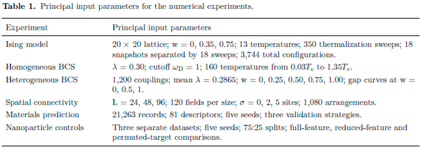
Ising model & 20 20 lattice; w = 0, 0.35, 0.75; 13 temperatures; 350 thermalization sweeps; 18 snapshots separated by 18 sweeps; 3,744 total configurations.Homogeneous BCS & = 0.30; cutoff = 1; 160 temperatures from to .Heterogeneous BCS & 1,200 couplings; mean = 0.2865; w = 0, 0.25, 0.50, 0.75, 1.00; gap curves at w = 0, 0.5, 1.Spatial connectivity & L = 24, 48, 96; 120 fields per size; = 0, 2, 5 sites; 1,080 arrangements.Materials prediction & 21,263 records; 81 descriptors; five seeds; three validation strategies.Nanoparticle controls & Three separate datasets; five seeds; 75:25 splits; full-feature, reduced-feature and permuted-target comparisons.
4. Results
4.1. Ising Observables and Phase Classification
Ising simulation results. Mean absolute magnetization and the within-chain fluctuation proxy are averaged across four test realizations at each disorder width, bands are standard errors across realizations. The vertical line represents the infinite-lattice reference value.
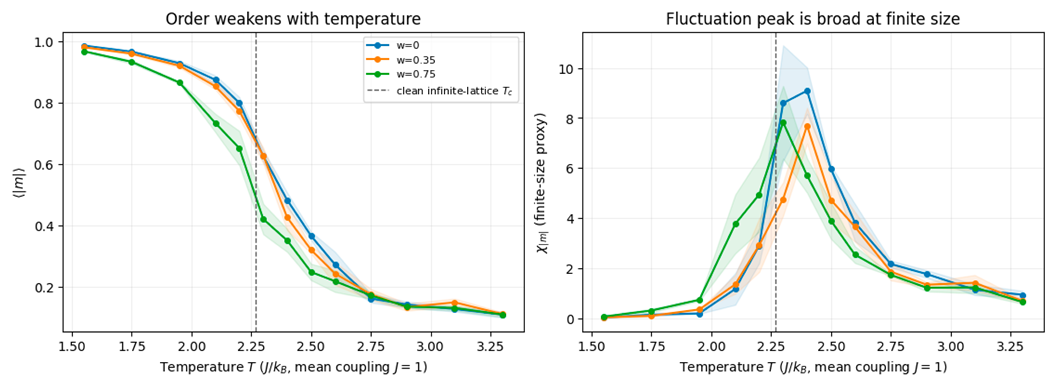
We find that fluctuation-proxy maxima occur at the grid temperatures 2.4, 2.4 and 2.3 for w = 0, 0.35 and 0.75, respectively, with their proxy values being 9.090, 7.694 and 7.826.
P0.31YYYY
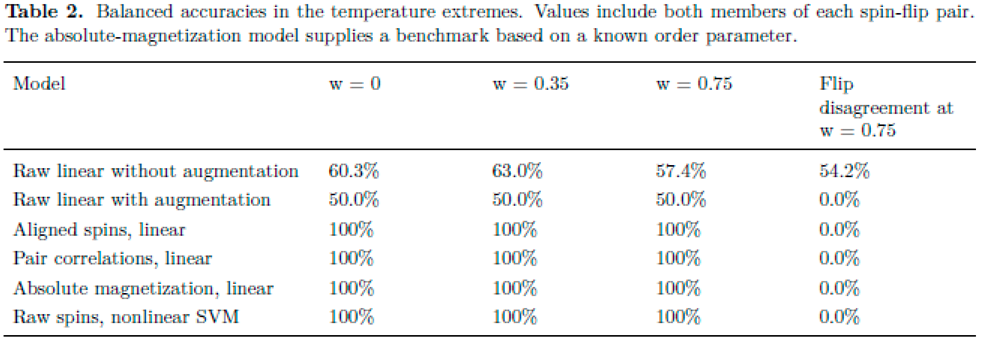
Model & w = 0 & w = 0.35 & w = 0.75 & Flip disagreement at w = 0.75
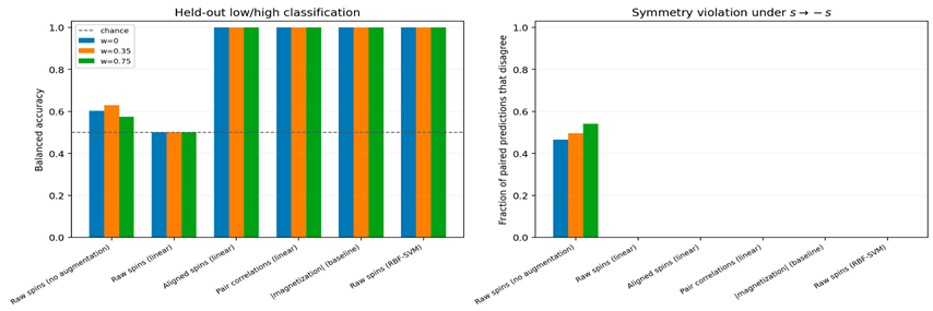
Raw linear without augmentation & 60.3% & 63.0% & 57.4% & 54.2%Raw linear with augmentation & 50.0% & 50.0% & 50.0% & 0.0%Aligned spins, linear & 100% & 100% & 100% & 0.0%Pair correlations, linear & 100% & 100% & 100% & 0.0%Absolute magnetization, linear & 100% & 100% & 100% & 0.0%Raw spins, nonlinear SVM & 100% & 100% & 100% & 0.0%
Our results show that invariant representations outperform the raw linear control in our experiments. They match the known order-parameter benchmark and nonlinear SVM in these regions.
4.2. Symmetry and Representation Geometry
Clean/disordered Ising benchmark: balanced accuracy and spin-flip consistency of contrasting input representations.
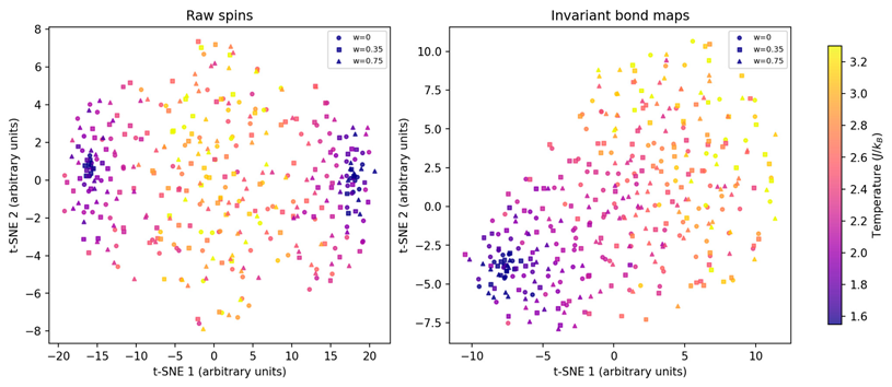
Ising t-SNE views of raw configurations vs. spin-flip-invariant bond features.
These raw configurations can be used to discern positive and negative magnetization regions which are part of the same ordered phase; sign-invariant features remove this distinction. Augmenting the raw linear model removed flip disagreement as well but that causes its accuracy to fall to chance. This therefore demonstrates why invariance and predictive information should be assessed together for these purposes; because of these considerations, we next work to make some database controls and perform nonlinear averaging tests.
4.3. Nonlinear Averaging of the BCS Model
Representations of BCS consistency and heterogeneity. In panel A we find that the supplied direct_t_c curve agrees with the finite-cutoff BCS solution rescaled by two; mean_t_c is shown without assigning its undocumented generation process. In B–D we can see new hypothetical scenarios use unit cutoff and fixed mean coupling. Mean gap, local paired fraction and mean local change as the prescribed distribution widens. B and C use .
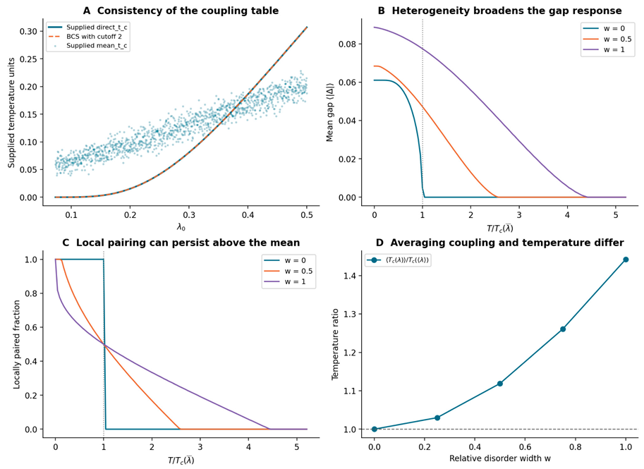
These results show that the fitted scale for direct_t_c is 2.000000000000; the maximum absolute residual is in the supplied temperature units here. As shown by this very close match, the table can be utilized as a robust solver benchmark: The original = 0.30 case is reproduced with = 0.04044953 and = 3.532249.
At fixed mean coupling 0.2865, the homogeneous transition temperature is 0.034570 and at full width w = 1, the mean local becomes 0.049861. This is a 44.23% increase while the maximum local is 0.153513; therefore, the broad distribution produces a long tail of local-pairing, demonstrating that averaging a nonlinear response differs from evaluating the response at the average input. The largest 96-versus-192-point gap difference in the specified check is . The largest relative mean-gap difference between 121 and 241 domains at the four checked temperatures is 0.283%.
4.4. Spatial Organization and Geometric Connectivity
Geometric connectivity of hypothetical locally paired domains. A–C: example L = 48 arrangements at approximately 55% occupancy; dark sites are occupied. Each has the same number of occupied sites and the same coupling distribution. D: spanning probability at L = 96. E: median spanning thresholds with central 95% realization ranges. F: mean occupied fraction at the spanning threshold. Smoothing widths describe the generating field, not a measured material length scale.
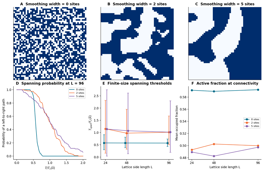
For L = 96, the unsmoothed arrangement has median= 0.572 and mean occupied fraction 0.592 at connectivity. Smoothing widths of two and five sites give median ratios 1.014 and 1.017. All three cases use the same marginal coupling values, so these differences arise from spatial placement within the prescribed model.
The correlated arrangements also exhibit broader realization-to-realization threshold ranges: the figure shows that median thresholds are not monotonic in smoothing width at every lattice size, and individual ranges overlap substantially. Figure 5 and Figure 6 demonstrate results that explain why an enhanced average local pairing scale does not necessarily need to determine macroscopic connectivity. The calculation provides a controlled analog for our discussion of graphs, heterogeneity and reduced descriptions.
4.5. Materials Generalization and Candidate Prioritization
Superconductivity database experiments. A: mean test RMSE with standard deviation over five split seeds. B: high-temperature-candidate recall against screening budget, with one-standard-deviation bands. C: row-level observed and predicted temperatures for the first chemical-system holdout; hexagon color indicates record count on a logarithmic scale. Here, the diagonal denotes exact agreement.
P0.22YYYYY
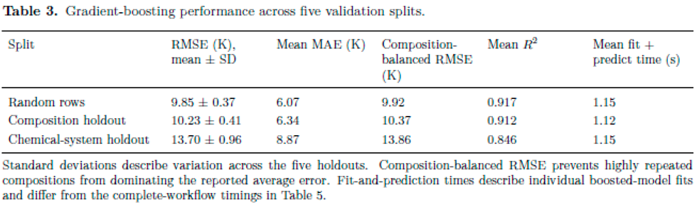
Split & RMSE (K), mean SD & Mean MAE (K) & Composition-balanced RMSE (K) & Mean & Mean fit + predict time (s)
Random rows & 9.85 0.37 & 6.07 & 9.92 & 0.917 & 1.15Composition holdout & 10.23 0.41 & 6.34 & 10.37 & 0.912 & 1.12Chemical-system holdout & 13.70 0.96 & 8.87 & 13.86 & 0.846 & 1.15
Standard deviations describe variation across the five holdouts. Composition-balanced RMSE prevents highly repeated compositions from dominating the reported average error. Fit-and-prediction times describe individual boosted-model fits and differ from the complete-workflow timings in Table 5.
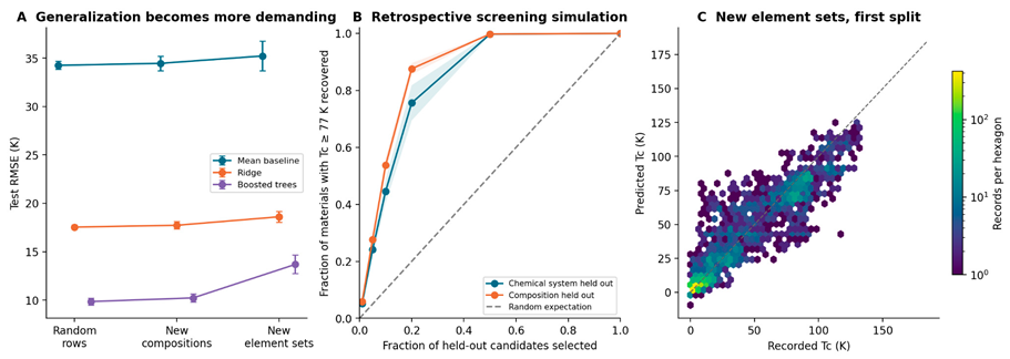
Random row splitting places test compositions already represented in training in 37.06% of test rows on average. The composition holdout removes this overlap, while the chemical-system holdout also removes every exact element-set match. The boosted model remains more accurate than ridge regression or a constant mean baseline in all three evaluation schemes, but its errors increase under the chemically stricter holdout.
Under chemical-system holdout selecting the top 10% of candidates gives mean precision 86.42%, compared with pool prevalence 19.55%. Mean enrichment is 4.45-fold and mean recall is 44.59%. Thus the model concentrates known high-temperature examples in a smaller candidate set. All rates use distinct held-out compositions.

4.6. Nanoparticle Feature Controls and Robustness
P0.22P0.23YYY
Dataset & Evaluation metric & Full features & only & Without 2,184 records & Balanced accuracy & 83.9% & 84.9% & 75.0%2,186 records & Mean absolute error & 20.69 & 19.10 & 23.292,187 records & Balanced accuracy & 99.2% & 96.1% & 90.6%
The mean absolute errors for the continuous-target dataset are expressed in the dataset’s recorded target units (whose physical interpretation has not been independently established). The high classification accuracy of the five-class dataset, particularly when using alone, indicates that the recorded labels are strongly associated with a restricted set of numerical descriptors.
For the sake of providing a negative control, the target labels were permuted during training. The resulting mean balanced accuracies were approximately 32.7% for the three-class dataset, 19.1% for the five-class dataset, which were near their respective chance-level baselines. The continuous-target model’s mean absolute error increased to approximately 50.21 under target permutation.
Robustness was additionally evaluated by adding Gaussian noise to test features, with noise standard deviations defined as fractions of each feature’s training-set standard deviation. At a noise level of 20%, balanced accuracy decreased from 83.9% to 79.5% for the three-class dataset. It also decreased from 99.2% to 84.2% for the five-class dataset. On the other hand, the continuous-target regression error increased from 20.69 to 21.40.
4.7. Computational Performance
P0.26YYYY
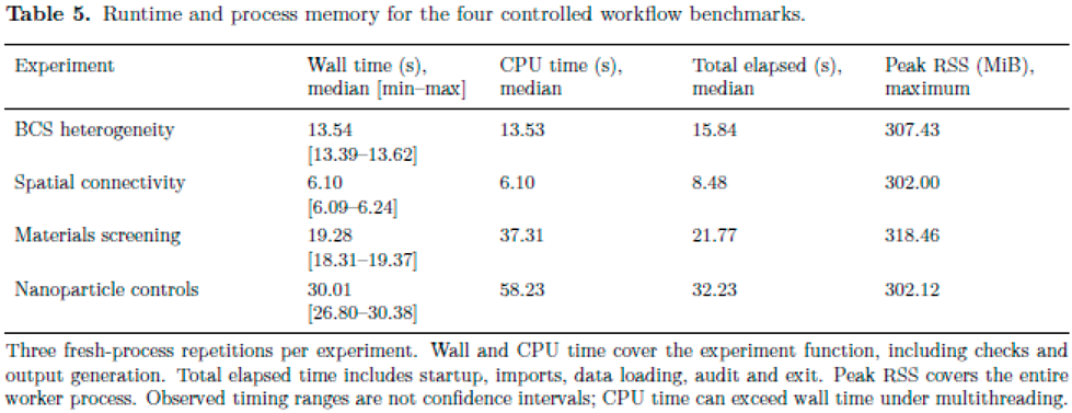
Experiment & Wall time (s), median [min–max] & CPU time (s), median & Total elapsed (s), median & Peak RSS (MiB), maximum
BCS heterogeneity & 13.54[13.39–13.62] & 13.53 & 15.84 & 307.43Spatial connectivity & 6.10[6.09–6.24] & 6.10 & 8.48 & 302.00Materials screening & 19.28[18.31–19.37] & 37.31 & 21.77 & 318.46Nanoparticle controls & 30.01[26.80–30.38] & 58.23 & 32.23 & 302.12
Three fresh-process repetitions per experiment. Wall and CPU time cover the experiment function, including checks and output generation. Total elapsed time includes startup, imports, data loading, audit and exit. Peak RSS covers the entire worker process. Observed timing ranges are not confidence intervals; CPU time can exceed wall time under multithreading.
5. Discussion and Limitations
The numerical studies we implement test three different related claims. First, the Ising example tests consistency under a known spin-flip symmetry. Second, the heterogeneous BCS and connectivity examples test what is lost when a distribution or a spatial pattern is replaced by its average. Third, the superconductivity database tests how the definition of a held-out material changes predictive performance and candidate prioritization.
We find that a symmetry-respecting representation can remove redundant distinctions while retaining informative observables. A nonlinear physical response can make mean-input approximations inaccurate even when every local calculation is correct. Separately, an ML model can predict historical measurements effectively while showing worse performance on chemically unfamiliar groups. The nanoparticle controls illustrate a further limitation, which is that labels which follow feature ranges can be easy to learn without supplying independent evidence of behaviors.
These experiments have several limitations that constrain interpretation. To begin with, the Ising design used for its study contains features such as a small lattice, four test realizations per disorder level, a coarse temperature grid, snapshots with unquantified autocorrelation, etc. Due to this, the fluctuation peaks we find cannot establish precise critical temperatures; likewise, perfect classification at temperature extremes does not demonstrate accuracy near the transition.
The BCS calculations prescribe a coupling distribution from a uniform parameter grid and treat domains independently, so enhanced local pairing scales do not establish an increase in bulk superconducting temperature. In a similar vein, the connectivity model excludes phase coherence, Josephson coupling, proximity effects, and transport. This makes its spanning thresholds strictly geometric instead of thermodynamic.
Materials prediction and screening are retrospective evaluations of known superconductors, with repeated compositions, conflicting recorded temperatures, and missing structural and synthesis information. Grouped holdouts reduce overlap but do not establish performance on genuinely new materials or experimental discovery rates. Variation across five overlapping holdouts measures sensitivity to the split rather than independent statistical uncertainty.
The benchmarks found from the performance tests demonstrate that the four new computational experiments are practical at the evaluated input sizes. Median experiment runtimes ranged from 6.10 to 30.01 seconds, with a maximum observed process memory usage of 318.46 MiB. These measurements include numerical checks and output generation, while memory measurements include imported libraries and loaded datasets. They therefore characterize the implemented workflows rather than isolated solver costs. Three timing repetitions on one shared CPU host establish observed execution variability, but provide limited evidence about performance on other hardware or at substantially larger scales.
The numerical validation supports reproducibility within the specified models. All 69 benchmark-generated tables reproduced their reference outputs without observed numerical differences. For the BCS calculations, increasing quadrature resolution produced a maximum checked gap difference of , while increasing domain resolution changed the mean gap by at most 0.283% at the tested temperatures. These checks support numerical stability over the evaluated conditions; they do not validate the underlying approximations against experimental superconductors. Similarly, verifying a geometric spanning threshold establishes connectivity under the prescribed occupancy rule, without demonstrating phase coherence or zero electrical resistance.
The materials-prediction results show that generalization depends strongly on how the test set is constructed. Mean RMSE increased from K for random row splits to K for composition holdouts and K for chemical-system holdouts, where uncertainties represent standard deviations across five splits. The larger error under chemical-system exclusion demonstrates the difficulty of transferring predictions to unfamiliar element combinations. Regardless, selecting the highest-ranked 10% of held-out compositions achieved 86.42% precision and 44.59% recall for the defined high-temperature screening target, supporting retrospective candidate prioritization. These results cannot establish prospective discovery performance, particularly given missing structural and synthesis information and the database’s restriction to known superconductors.
The nanoparticle controls further qualify the interpretation of high predictive accuracy. The five-class model achieved 99.23% balanced accuracy using all features, while S alone achieved 96.09%; the latest permuted-target control returned 19.09%, close to the 20% chance reference. These findings demonstrate strong associations between the descriptors and recorded labels, but do not establish their physical origin or prove label leakage. At the largest tested feature-noise level, balanced accuracy decreased to 84.21%, showing that near-perfect performance on unperturbed inputs does not imply equivalent robustness to input uncertainty. Independent verification of feature definitions, units, and label-generation procedures remains necessary before interpreting these categories as physical phases.
The earlier Ising and t-SNE experiments were excluded from the new runtime benchmark, so its timing conclusions do not extend to those methods. High classification accuracy in temperature regions far from the transition demonstrates discrimination between the selected states, but does not establish precise critical-point identification. Likewise, t-SNE provides an exploratory representation of high-dimensional structure; visual separation alone cannot establish a thermodynamic transition. Stronger physical conclusions require targeted sampling and finite-size analyses, models incorporating phase coupling or transport, and validation against independently measured materials.
Taken together our literature review, experiments, and analytics support controlled comparisons of representations, heterogeneity, and validation choices rather than establishing a general superconducting mechanism or experimentally verified materials-design strategy. All results should be interpreted with caution due to biases and limitations with simulation parameters and datasets used.
6. Conclusion
This paper examined how numerical computation and simulations, ML, and various representations of physical systems can be used to study the behavior of phase transitions and states in superconducting materials, especially those in a disordered system. The previous literature overview and computational experiments support the framework of using dimensional reductions, continuum models, data-driven representations, and numerics to examine these systems.
Mathematical tricks exploiting symmetries, correlated interactions, spatial organization, nonlinear dynamics, and validation design can improve the robustness of a model and influence what can be learned from it. From the Ising and numerical BCS demonstrations, Ising experiments with incorporated spin-flip symmetries, connectivity experiments, and critical-temperature prediction and error analysis we demonstrate how phase classification can be guided, how variables like spatial connectivity affect how we must represent a system, and how we can validate results towards a specific application and interpretation.
The runtime measurements and numerical checks used to benchmark our compute and experimental design provide practical feasibility and reproducibility to the framework and scales proposed. To address limitations within these areas, further work should be done on larger lattice-models, quantification of sampling correlations, incorporate interactions between superconducting regions, and evaluate predictions using independently characterized materials.
References
- Bardeen, J.; Cooper, L. N.; Schrieffer, J. R. Theory of superconductivity. Phys. Rev. 1957, 108(5), 1175–1204. [Google Scholar] [CrossRef]
- Cao, Z.; Barati Farimani, O.; Ock, J.; Barati Farimani, A. Machine learning in membrane design: From property prediction to AI-guided optimization. Nano Lett. 2024, 24(10), 2953–2960. [Google Scholar] [CrossRef] [PubMed]
- Dodaro, J. F.; Kivelson, S. A. Generalization of Anderson’s theorem for disordered superconductors. Phys. Rev. B 2018, 98(17), 174503. [Google Scholar] [CrossRef]
- Dong, X.-Y.; Pollmann, F.; Zhang, X.-F. Machine learning of quantum phase transitions. Phys. Rev. B 2019, 99(12), 121104(R). [Google Scholar] [CrossRef]
- Dubi, Y.; Meir, Y.; Avishai, Y. Nature of the superconductor–insulator transition in disordered superconductors. Nature 2007, 449(7164), 876–880. [Google Scholar] [CrossRef] [PubMed]
- Dubi, Y.; Meir, Y.; Avishai, Y. Island formation in disordered superconducting thin films at finite magnetic fields. Phys. Rev. B 2008, 78(2), 024502. [Google Scholar] [CrossRef]
- Erpelding, M.; Braemer, A.; Gärttner, M. Exploiting emergent symmetries in disorder-averaged quantum dynamics. Phys. Rev. B 2026, 113(14), 144206. [Google Scholar] [CrossRef]
- Hamidieh, K. A data-driven statistical model for predicting the critical temperature of a superconductor. Comput. Mater. Sci. 154 2018a, 346–354. [Google Scholar] [CrossRef]
- Hamidieh, K. Superconductivty data [Data set]. In UCI Machine Learning Repository; 2018b. [Google Scholar] [CrossRef]
- Ju, Y.; Alam, S.S.; Minoff, J.; Anselmi, F.; Pu, H.; Patel, A. Interpreting convolutional neural networks’ low-dimensional approximation to quantum spin systems. Phys. Rev. Res. 2025, 7(1), 013094. [Google Scholar] [CrossRef]
- Obernolte, P.; Dranczewski, J.; Yin, Y.; Farchy, T.; Ng, W. K.; Simonsen, T.; Großhauser, E.; Arnaudon, A.; Peach, R. L.; Barahona, M.; Sapienza, R.; Gartside, J. C.; Raziman, T. V. Graph-theoretic design of lasing networks for physical vision [Preprint]. arXiv 2026. [Google Scholar] [CrossRef]
- Rende, R.; Viteritti, L. L.; Georges, A. Superconductivity in the t–t′ Hubbard model from symmetry-preserving neural-network quantum states [Preprint]. arXiv 2026. [Google Scholar] [CrossRef]
- Sacépé, B.; Chapelier, C.; Baturina, T. I.; Vinokur, V. M.; Baklanov, M. R.; Sanquer, M. Disorder-induced inhomogeneities of the superconducting state close to the superconductor-insulator transition. Phys. Rev. Lett. 2008, 101(15), 157006. [Google Scholar] [CrossRef] [PubMed]
- Scikit-learn developers. GroupShuffleSplit [Documentation for scikit-learn 1.8.0]. n.d.-a. Available online: https://scikit-learn.org/1.8/modules/generated/sklearn.model_selection.GroupShuffleSplit.html.
- Scikit-learn developers. HistGradientBoostingRegressor [Documentation for scikit-learn 1.8.0]. n.d.-b. Available online: https://scikit-learn.org/1.8/modules/generated/sklearn.ensemble.HistGradientBoostingRegressor.html.
- Tsai, Y.-C.; Chang, Y.-Y.; Hsu, T.-Y.; Kuo, T.; Kuo, C.-N.; Lue, C.-S.; Chiu, K.-L.; Hsu, C.-H.; Ke, C.-T. Field-controlled breaking and restoration of parity-time symmetry in Josephson interference. arXiv 2026. [Google Scholar] [CrossRef]
- van der Maaten, L.; Hinton, G. Visualizing data using t-SNE. J. Mach. Learn. Res. 9 2008, 2579–2605. Available online: https://jmlr.org/papers/v9/vandermaaten08a.html.
- Wetzel, S. J. Unsupervised learning of phase transitions: From principal component analysis to variational autoencoders. Phys. Rev. E 2017, 96(2), 022140. [Google Scholar] [CrossRef] [PubMed]
- Wines, D.; Choudhary, K.; Biacchi, A. J.; Garrity, K. F.; Tavazza, F. High-throughput DFT-based discovery of next generation two-dimensional (2D) superconductors. Nano Lett. 2023, 23(3), 969–978. [Google Scholar] [CrossRef] [PubMed]
Disclaimer/Publisher’s Note: The statements, opinions and data contained in all publications are solely those of the individual author(s) and contributor(s) and not of MDPI and/or the editor(s). MDPI and/or the editor(s) disclaim responsibility for any injury to people or property resulting from any ideas, methods, instructions or products referred to in the content. |
© 2026 by the authors. Licensee MDPI, Basel, Switzerland. This article is an open access article distributed under the terms and conditions of the Creative Commons Attribution (CC BY) license (http://creativecommons.org/licenses/by/4.0/).
Copyright: This open access article is published under a Creative Commons CC BY 4.0 license, which permit the free download, distribution, and reuse, provided that the author and preprint are cited in any reuse.