
Submitted:
16 November 2026
Posted:
17 November 2026
Read the latest preprint version here
Abstract
Point-particle kinematics and projective measurement rely on two unbounded idealizations: exact spatial localization at finite energy and instantaneous collapse at infinite bandwidth. We formulate nonrelativistic quantum mechanics in canonical density–phase variables paired with a falsifiable information-capacity hypothesis. Axiom takes an objective configuration density and compact phase field with finite spatial Fisher information, quantized vortex circulation, and simple nodal phase matching as explicit kinematic inputs, ruling out point localization and addressing Wallstrom’s objection. Axiom combines the Fisher localization energy with a Nyquist–Planck ceiling: for a declared memoryless port, the conditional information rate cannot exceed its entangling energy dispersion divided by Planck’s constant. On regular charts, the density–phase manifold carries a weak Kähler structure isometric to the Fubini–Study metric; with explicit form-domain and unitary-lift inputs, the closed limit recovers Schrödinger dynamics, bound-state spectra, and uncertainty relations. Under bounded continuous monitoring, the stochastic filter is globally well posed: isolated quantum nondemolition monitoring selects outcomes with Born weights from Postulate , and deterministic bare rates yield linear Lindblad evolution and local no-signaling. A buffered record-plus-Holevo extension gives a falsifiable circuit-QED test on damped ports while exposing an open dynamical boundary in undamped pointer generation.
Keywords:
quantum foundations
; information geometry
; Fisher information
; continuous quantum measurement
; channel capacity
; circuit quantum electrodynamics
1. Introduction
Quantum mechanics predicts measurement statistics accurately, yet its formulations assign different physical meanings to the quantum state and to measurement-induced state reduction. Operationally, classical point-particle mechanics and textbook projective measurement rely on two implicit idealizations: unbounded spatial localization, associated with the use of exact real-valued classical coordinates [1,2] and with point localization at finite classical kinetic energy, and infinite measurement bandwidth, which allows an apparatus to extract finite state-distinguishing information instantaneously during collapse. Hydrodynamic and Fisher-information reconstructions express quantum dynamics in terms of a probability density and a phase field on configuration space, linking quantum dynamics to classical fluid flow, entropic dynamics, and statistical geometry [3,4,5,6,7,8,9,10,11]. Two structural gaps nevertheless persist in local hydrodynamic formulations: local density–phase partial differential equations do not enforce the global multivaluedness and nodal matching conditions required by single-valued wave functions [12,13], and adjoining an instantaneous projection postulate leaves unspecified the physical rate at which a finite-energy interaction can transfer information into an apparatus record.
The density–phase formulation developed here addresses both idealizations through two explicit axioms that separate inherited quantum-mechanical structure from an empirical rate-limit hypothesis. Axiom 1 adopts an ontic pure-state description [14,15] in which a microscopic pure state is the objective field pair on configuration space with no underlying point-particle coordinate. The Madelung map links this field pair to its Hilbert-space representation. Requiring finite spatial Fisher information introduces an intrinsic localization kinetic energy that scales as when a fixed-shape density profile is compressed to spatial width ℓ, ruling out unbounded spatial localization precision at finite energy. Because finite Fisher and flow energies alone do not quantize vortex circulation or fix sign changes across nodal surfaces, Axiom 1 imposes integer (or spinorial half-integer) circulation and cusp-plus- phase matching across simple nodal hypersurfaces as explicit kinematic inputs rather than consequences of local hydrodynamics, thereby addressing Wallstrom’s objection axiomatically.
To replace the idealization of infinite measurement channel bandwidth with a finite-rate hypothesis, Axiom 2 postulates a Nyquist–Planck ceiling on the predictable conditional information rate of each declared hardware port . Classical Shannon, quantum Holevo, and physical information-processing bounds constrain coding rates and accessible information [16,17,18,19,20], but they do not derive a Hamiltonian time-rate ceiling from interaction energy dispersion; we therefore formulate this bandwidth ceiling as an independent, empirically falsifiable hypothesis rather than a theorem of standard quantum mechanics. Building on continuous quantum filtering, quantum-state diffusion, and stochastic reduction theory [21,22,23,24,25,26,27], finite-bandwidth monitoring governs the stochastic evolution of , driving conditional variance decay and asymptotic Born-rule outcome selection while yielding linear Gorini–Kossakowski–Sudarshan–Lindblad (GKSL) master equations for nonselective ensembles. Because the information extraction rate vanishes whenever the measurement coupling is turned off, state reduction in this formulation is apparatus-conditioned, avoiding the background diffusion and spontaneous heating characteristic of universal collapse models [28,29,30].
Our mathematical development builds on informational, Fisher-information, and geometric formulations of quantum mechanics [31,32,33,34,35,36,37,38,39,40] while maintaining a clear distinction among three levels of results. On regular positive-density charts, exact weak Kähler identities connect the Fisher–Rao metric and canonical symplectic form to the projective Fubini–Study metric and closed Schrödinger dynamics. Global Hilbert-space completion across nodal sets, self-adjoint generator lifts, and initial propensity probabilities require additional analytical inputs and are stated explicitly as domain assumptions and postulates. The Nyquist–Planck capacity ceiling, its operator-Schmidt multi-port calibration, and its circuit-QED scaling laws constitute empirical hypotheses open to laboratory falsification.
Section 2 formulates Axioms 1 and 2, geometric normalization, operator-Schmidt accounting, global form domains, and the Madelung–Kähler and operator correspondences. Section 3 derives momentum-covariance and covariance-entropy bounds, closed Schrödinger equivalence, standard bound-state spectra, and global stochastic filtering results covering Sobolev regularity, martingale Born-weight convergence, measurement backaction power, and local completely positive trace-preserving (CPTP) ensemble no-signaling. Section 4 establishes finite-time localization and binary quantum nondemolition (QND) readout horizons, proves a coherent-pointer Holevo storage budget, and evaluates dispersive superconducting circuit quantum electrodynamics (cQED) benchmarks against the rapid readout experiment of Walter et al. [41]. Section 5 summarizes the theoretical scope, mathematical boundaries, and experimental outlook, with broader extensions treated in the companion preprint [42].
Table 1 maps the manuscript’s logical layers, separating inherited quantum-mechanical structures, explicit analytical inputs, operational results, and falsifiable empirical hypotheses.
2. Axiomatic Framework and Information Geometry
Throughout this paper, axioms and postulates specify the adopted physical and probabilistic structure, assumptions state the conditions under which mathematical results hold, hypotheses denote additional empirical claims subject to experimental falsification, and propositions establish supporting analytical, regularity, or operational results alongside the main theorems. These labels indicate logical roles rather than degrees of certainty. The capacity ceiling included in Axiom 2 is an empirical hypothesis, as is its buffered extension in Hypothesis 1.
2.1. Geometric Calibration and Information Measures
The framework distinguishes three information-theoretic quantities that characterize spatial localization, phase-space dispersion, and open-channel measurement throughput: spatial Fisher information, covariance-based phase-space entropy, and conditional information extracted by a measurement record.
For a two-level pure state, the Braunstein–Caves normalization relates the quantum Fisher metric to the Fubini–Study line element via [47,48,49]. The corresponding Bloch sphere has total solid angle . Treating steradians as dimensionless, we define the calibration constants
where is the reciprocal solid-angle factor (formally ) and j is a conventional reference information threshold organizing the geometric factors and relative to h (rescaling this threshold shifts the time-horizon convention linearly without fixing the capacity prefactor). Throughout, we treat the natural-logarithm unit as dimensionless when relating information rates to inverse time, while distinguishing information throughput rates (in ) from electrical hardware bandwidths (in ).
On configuration space , a normalized density carries spatial Fisher information with dimensions of inverse length squared. To quantify joint phase-space dispersion from the symmetrized position–momentum covariance matrix , we define the effective spread and the Gaussian-reference covariance entropy relative to the quantum cell by
Unlike von Neumann entropy or marginal differential entropies, depends solely on second-moment phase-space volume; a pure minimum-uncertainty Gaussian state has while satisfying .
Whereas an individual pure state is specified by the objective field pair , statistical mixtures and unmonitored environmental couplings are represented by the configuration-space coherence kernel
whose diagonal gives the configuration density and whose off-diagonal elements encode spatial phase coherence. Under any ensemble decomposition, the total momentum variance obeys the law of total variance , while the linear nonselective master equation (70) (Section 3.4) depends only on the kernel rather than on a preferred pure-state decomposition [50,51,52,53,54].
Along an ideal QND observation filtration , let denote the pathwise predictable entropy compensator. In the discrete-branch Shannon model of Theorem 7, the mutual information extracted by the measurement record up to time t equals the ensemble expectation , linking the trajectory-level compensator to the ensemble information gain. Throughout the paper (developed in Section 3.4, Section 3.5, and Section 4.2), [Eq. (72)] and [Eq. (93)] both denote this classical Shannon mutual information between the discrete QND label K and the continuous observation record up to time t (with its multi-port generalization in Eq. (76)), distinct from the conditional Holevo pointer storage in Eq. (93) and the single-shot accessible information illustrated in Eq. (94).
2.2. Objective Fields and Nodal Topology
Axiom 1
(Objective fields and nodal topology). The objective microscopic state on a configuration manifold M is a field pair with no classical point-particle coordinate. Here is a normalized density and is a flat phase section on the positive support , with local phases identified modulo h, values on unassigned, and overall constant phase shifts quotiented out.
- The amplitude satisfies , the flow field satisfies , and second position moments are finite whenever invoked, ensuring finite spatial Fisher information and excluding pointlike concentration at finite energy.
- Around every closed loop , the phase gradient obeys the circulation conditionwhere χ specifies the flat line-bundle sector. In the scalar sector (), circulation around a codimension-two vortex is , whereas sectors with holonomy use a character taking values 0 and modulo one (full multicomponent spin- structure is deferred to the companion preprint [42]).
- Across a codimension-onesimple, locally real-phase nodal hypersurface where the signed amplitude admits the normal expansion () in a local normal coordinate s, the one-sided limits satisfyproviding first-order () matching of the signed section across simple nodal walls (higher regularity follows from domain or section conditions rather than Eq. (5) alone), while allowing general complex sections to exhibit higher-codimension nodal sets.
Figure 1 illustrates the two topological constraints of Axiom 1: quantized loop circulation (4) restricts the multivalued phase around codimension-two vortices, whereas nodal matching (5) pairs a symmetric modulus cusp with a phase jump of an odd multiple of across a simple codimension-one wall.
Remark 1
(Ontological status and axiomatic treatment of Wallstrom’s objection). A microscopic system has no classical pointlike position at any time ; this reflects its objective field ontology rather than epistemic ignorance of hidden point coordinates. Without assuming internal material substructure, Axiom 1 specifies how the system is represented and manifests in interactions with other physical systems on its configuration manifold M.
Finite Fisher and flow energies alone do not quantize vortex circulation: on , the trial fields and carry finite kinetic energy for every real . Equation (4) rules out noninteger scalar-sector circulation as an explicit topological input. Related discussions of the quantization gap and proposed additional conditions appear in [12,13,43,55,56]. Likewise, Eq. (5) combines the modulus cusp with the phase factor to reconstruct a -matched signed section across simple nodes.
2.3. Hamiltonian Dynamics, Monitoring, and Channel Capacity
Axiom 2
(Hamiltonian dynamics, monitoring, and channel capacity). Consider a particle of mass in a real scalar potential coupled to a declared diffusive measurement channel for a real-valued observable (distinct from the configuration manifold M of Axiom 1), with conditional mean and variance .
- In the nonrelativistic quadratic regime, the conservative Hamiltonian functional and second-moment momentum constitutive law are
- Empirical capacity hypothesis.Each physical readout port is declared prior to data analysis by its system–environment partition, interaction Hamiltonian, probe state, bath correlation scale, collection efficiency, amplification quadrature, and admissible state domain. For a memoryless (direct) readout port, the predictable conditional information rate obeys the Nyquist–Planck ceilingwhere is the standard deviation of the centered entangling interaction [Eq. (96), Section 4.3], and independent parallel hardware ports with orthogonal innovations obey additive accounting, . Inequality (8) sets a kinematic rate ceiling without prescribing a unique saturation mechanism. When an intermediate coherent pointer buffers distinguishability between the entangling source and the detected output (as in dispersive cQED), Hypothesis 1 [Eq. (95)] extends this ceiling to the joint classical–quantum (cq) information increment—detected record mutual information plus residual conditional Holevo pointer storage (Section 4.2).
- Where , the monitored density and phase fields obey the coupled Itô equationswith for pure configuration monitoring and with the bare-rate calibration (12) providing a nonsingular continuation of Eq. (9) across . Continuous monitors satisfy the stated moment and gradient integrability conditions, global form-domain solutions use bounded smooth monitors, and discrete QND monitoring follows Assumption a (Section 2.4).
- For time-independent V, closed Hamiltonian transport conserves H. Because convective flow and potential energies are linear in ρ, the expected system-side measurement work under pure configuration monitoring arises entirely from the Fisher localization energy,while the full apparatus energy balance also includes probe driving and amplifier reservoirs.
Remark 2
(Rate calibration and operator-Schmidt accounting). A calibrated detector with deterministic bare measurement rate satisfies
This calibration rewrites the density innovation in Eq. (9) as , preserving normalization without dividing by and yielding the linear GKSL ensemble master equation (70) for deterministic bare rates.
On a product reference state , equip the real spaces of centered Hermitian operators modulo their zero-variance kernels with the positive-definite symmetrized covariance inner products and . The centered bilinear interaction admits the covariance-weighted operator-Schmidt decomposition
whose singular values define the nuclear-norm multi-port capacity scale and symmetrized Frobenius energy scale:
When the canonical Schmidt modes correspond to independently monitored physical ports, applying Axiom 2 mode by mode yields .
With and , the operator product identity yields the exact product-state variance relation and norm bounds
The joint energy variance coincides with whenever the commutator cross-term vanishes (including rank-one couplings and commuting system or probe quadratures), but can differ for noncommuting multi-mode interactions: for on , destructive interference gives , whereas and .
For a linear bath coupling with symmetric bath correlation and integrable spectrum , the equal-time dispersion , total dephasing rate , effective readout rate (reducing to at unit efficiency ), and bath correlation time separate instantaneous energy fluctuations from Markovian readout strength. Monitoring the conjugate amplification quadrature instead generates stochastic phase backaction [59],
contributing standard linear dephasing to the nonselective master equation.
Proposition 1
(Conditional uniqueness of the Fisher localization energy). Let a local nonnegative localization kinetic cost take the form . Under continuity, Euclidean invariance, quadratic scale covariance, zero cost for uniform densities, and pointwise additivity for independent product subsystems,
one has . Axiom 2(1) specifies the scale constant as a constitutive input, giving
while the unitary quantum-Fisher speed limit calibrates the dimensional rate scale of the Nyquist–Planck bound (8).
Proof.
Setting or shows that is independent of density and dimension, and Cauchy’s functional equation with continuity and nonnegativity yields , matching quadratic spatial scaling [8,9,60,61,62].
Under coherent unitary evolution, the horizontal projective velocity has norm , so the Mandelstam–Tamm quantum-Fisher speed bound [49,63,64] gives
By contrast, substituting the density innovation of Eq. (9) into yields the diffusive quadratic variation . Because ballistic unitary arc length and diffusive increments have distinct stochastic orders [65], Eq. (19) calibrates the dimensional unit while leaving the diffusive bandwidth ceiling (8) as an independent empirical hypothesis. □
2.4. Domains, Probability Semantics, and Topological Conservation
Assumption A1
(Energy domain and boundary conditions). Fix M, boundary conditions, and a flat line-bundle sector . Write with , and assume has relative form bound below one with respect to the kinetic-plus- form. The closed semibounded quadratic form
defines the self-adjoint Friedrichs realization , with incorporating the chosen boundary conditions (replaced by for Dirichlet boundaries). Under this construction, if and only if and some satisfies for all , in which case .
Admissible finite-energy states are normalized sections in with finite second position moments when required. Sobolev regularity is imposed on the complex section ψ rather than on alone, since a smooth vortex section can lie in while . On , integrations by parts use smooth cutoff limits justified by regularity and finite second moments.
Assumption A2
(QND isolation or measurement dominance). Quantitative variance-decay bounds are evaluated in two operational regimes:
- (a)
- In strict discrete QND monitoring, the normal boundary flux vanishes, and has distinct branch eigenvalues on disjoint supports (grouping degenerate subspaces into single branches) and branch projections that preserve and commute with .
- (b)
- For a continuous observable with Hamiltonian variance drift , neglecting convective variance transport requires the dominance condition (), which can be checked, for linear position monitoring in a quadratic potential, using the coupled Gaussian covariance equations (80) (Section 4.1).
Postulate 1
(Objective propensity probabilities). The configuration density defines single-case propensities , including initial branch priors at the onset of a QND measurement. Entanglement envariance motivates equal priors for equal-norm Schmidt branches [66,67], though its foundational premises require physical interpretation [68]; we therefore posit Postulate 1 directly as the formulation’s probability bridge.
In analogy with coarse-grained H-theorems in hydrodynamic foundations [69,70], relative-entropy monotonicity holds whenever coarse-grained sampling and propensity densities share an advection–diffusion closure with positive-definite diffusion tensor and vanishing boundary flux:
Differentiating cancels the shared Liouville advection terms, and integration by parts yields the dissipation integral in Eq. (21); whenever the nonnegative dissipation integral is at least (), Pinsker’s inequality implies exponential relaxation, .
Proposition 2
(Circulation and nodal kinematics). Under pure configuration monitoring, any closed loop C remaining inside the regular region conserves its circulation:
On any oriented two-dimensional transverse cross-section, the winding-number sum of isolated codimension-two vortex cores is likewise invariant under smooth homotopies without boundary crossings. Near a nondegenerate fold where a locally real amplitude expands as (), pairs of simple zeros nucleate or annihilate at , whereas measurement-only updating multiplies the section by a strictly positive likelihood factor and preserves its nodal set.
Proof.
Exactness of the gradient drift in Eq. () yields Eq. (22), and homotopy invariance preserves the total vortex index. Setting in the fold expansion gives the root locus , while positivity of the measurement likelihood multiplier follows from Proposition 3 (Section 3.4). □
5
2.5. Madelung–Kähler Geometry and Operator Correspondence
Theorem 1
(Regular-chart Madelung–Kähler correspondence). On compact M with , consider normalized densities bounded away from zero and local phase variations modulo constants. On the horizontal tangent bundle defined by and , equip the -paired cotangent chart with the following forms [35,39,40,43]:
and define the almost-complex operator and Madelung map
Proof.
Direct evaluation gives , , and , with J preserving both horizontal constraints and closed. Differentiating yields
Taking the inner product of two such variations gives Eq. (25), with inverse differential and . The complex section chart provides integrability, while the metric is weak relative to the topology.
On , fix a normalized Gaussian with density and form the unital Banach algebra (). For with and , set
Reciprocal, square-root, and phase maps are smooth on this weighted chart with . Because , Gaussian decay places these states inside the operator domains of the free, harmonic, and three-dimensional Coulomb Hamiltonians; when nodes develop, global continuation proceeds in the complex form domain of Assumption A1. □
Theorem 2
(Conditional operator correspondence and premeasurement). Fix and its projective completion. Any global one-parameter projective Kähler symmetry admitting a strongly continuous unitary lift has a unique self-adjoint generator for the chosen lift [71]. Different unitary lifts of the same projective flow change by an additive scalar multiple of the identity. For self-adjoint on a common invariant dense domain in , the expectation functionals and satisfy
For , the premeasurement coupling translates branch pointers by , yielding detector branch weights whenever the displaced pointer supports are disjoint.
Proof.
Stone’s theorem yields under the unitary lift hypothesis. With , the horizontal vector field is , and Eq. (25) gives , establishing Eq. (28) (so matches ). Under , the commutation relation ensures that each branch norm is preserved, while the corresponding pointer shifts by . Disjointness holds when the initial pointer support diameter lies below , whereas smooth Gaussian pointers retain nonvanishing tail overlap at any finite interaction impulse . Because noncommuting observables require distinct premeasurement couplings, their outcome statistics are context-dependent and need not admit a single noncontextual joint probability distribution [72,73,74,75]. □
3. Nonrelativistic Kinematics and Continuous Measurement
We now establish closed-system kinematic bounds, Schrödinger equivalence, and standard bound-state spectra, followed by global stochastic filtering and ensemble dynamics. Global trajectories are defined on and reduce to the density–phase equations (9) and () wherever .
3.1. Momentum Covariance, Uncertainty, and Phase-Space Entropy
Theorem 3
(Momentum covariance, uncertainty, and covariance entropy). Under Assumption A1, let be normalized and have finite second moments of position and momentum. Set
The symmetrized momentum covariance decomposes as
giving for . For , the position–momentum covariance matrix Σ obeys
where equality in the determinant bound holds if and only if ρ is Gaussian and is affine, and equality in the product bound additionally requires .
In any dimension , and the Gaussian-reference covariance entropy relative to satisfies
Proof.
Writing gives the weak derivative
whose gradient inner product has a real part that separates into phase and amplitude terms. Using almost everywhere and subtracting proves Eq. (30) across nodes.
For , cutoff integration by parts and Cauchy–Schwarz yield the Cramér–Rao bound [62]:
with equality if and only if (Gaussian ). Substituting Eq. (30) gives
where the first term vanishes precisely when , proving the Robertson–Schrödinger bound [76,77].
For , positivity of the Gram matrix of on Schwartz sections and by closure on the second-moment domain gives
Williamson’s symplectic diagonalization [78] transforms by symplectic congruence to a positive matrix with eigenvalue pairs , hence . Its determinant gives the first bound below. Applying the one-dimensional uncertainty bound to each canonical pair and then Cauchy–Schwarz gives the second bound. Thus
where and . Inserting the determinant bound from Eq. (37) into Eq. (2), with , gives Eq. (32). □
The proof of Eq. (34) on uses a vanishing integration-by-parts boundary term. On a bounded interval the boundary term must also be checked, as a uniform Neumann eigenstate on has . Under shape-preserving compression , the Fisher information scales as , so the localization energy diverges as , excluding pointlike spatial localization at finite kinetic energy.
3.2. Resolution Time and Closed-System Schrödinger Equivalence
Theorem 4
(Conditional channel-resolution time bound). For a declared memoryless channel satisfying Eq. (8) on its admissible state domain,
In the finite QND model where , taking expectations gives the ensemble budget
Whenever holds deterministically on , acquiring the calibration reference unit —whether as an ensemble threshold or a pathwise threshold —requires
Proof.
Equation (40) replaces the instantaneous state reduction of an idealized infinite-bandwidth measurement channel with a finite acquisition horizon inversely proportional to . At fixed energy dispersion , resolving one reference unit j requires at least , a time shorter by a factor of than the Mandelstam–Tamm orthogonalization bound [63], whereas resolving one Shannon bit () requires . These bounds govern distinct physical processes: open-channel information extraction versus unitary state orthogonalization [63,79] or finite-time state discrimination [80].
Theorem 5
(Closed-limit Schrödinger equivalence). For the self-adjoint Hamiltonian of Assumption A1, closing all measurement ports (, ) renders the density–phase equations equivalent to
pointwise on regular positive-density regions; globally on , the evolution is defined by the unitary group with and . For a one-dimensional Gaussian wave packet in an at-most-quadratic potential, the centroid and width obey
These equations also govern the Gaussian variational projection in general smooth potentials.
Proof.
A compactly supported variation inside gives
This gives the Bohm potential . In the closed limit, the density–phase equations (9) and () become
matching the real and imaginary parts of Eq. (41). Across nodes, the unitary trajectory satisfies the regularity conditions and , as well as the weak formulation
which avoids division by and reduces to the strong operator equation on . This form-domain flow provides the global continuation across nodal sets.
For , continuity fixes the quadratic phase
5
3.3. Oscillator, Orbital-Angular-Momentum, and Hydrogen Spectra
Theorem 6
(Oscillator, orbital-angular-momentum, and hydrogen spectra). Under the standard self-adjoint harmonic-oscillator, spherical angular-momentum, and Coulomb realizations, Axiom 1 and Theorem 5 yield the exact bound-state spectra:
For ,
For a central potential, simultaneous orbital eigenstates satisfy
For hydrogen, with and , completing the square gives
with the unique ground-state density and excited spin-free levels
Proof.
For the oscillator, setting and yields Hermite’s equation and recurrence:
Terminating the series at produces the Hermite polynomials and makes u square-integrable. Equation (5) matches signs across simple nodes, and the virial identity gives Eq. (47).
These results confirm closed-sector compatibility with standard quantum mechanics, where the competition between Coulomb attraction and Fisher localization energy stabilizes the atom at the Bohr radius .
3.4. Global Stochastic Evolution, Born Weights, and the Master Equation
Throughout this subsection, denotes a deterministic, locally integrable bare rate with integrated exposure and predictable information rate . The observation record is related to the innovation Wiener process in Eq. (9) by .
Proposition 3
(Measurement-only Sobolev regularity). Let a normalized state and a real function satisfy (ensuring finite second variance moments) and . Without Hamiltonian transport, consider the observation process
where X is an auxiliary random variable realizing the marginal observation law. For finite and finite , the posterior section
remains in and satisfies the exact mean-energy identities
Proof.
Completing the square bounds and , so the weak product rule gives
With denoting the centered Gaussian density of variance , the record density is and satisfies . Averaging cancels and reduces to the variance of the shifted Gaussian variable, proving Eq. (56) without dividing by at nodes. □
Proposition 4
(Global form-domain evolution with bounded monitors). Let be the time-independent semibounded Schrödinger operator of Assumption A1 on , choose c so that , and equip with . For real and normalized , the stochastic Schrödinger equation
admits a global, pathwise unique, adapted mild solution with continuous sample paths and . For every and ,
and the mean energy satisfies
If and , the solution has continuous graph-norm paths in and satisfies Eq. (58) strongly in .
Proof.
Related stochastic regularity methods are developed in [44]. Because are bounded multipliers on , passing to the interaction picture with yields locally Lipschitz coefficients on . Itô’s formula preserves , bounding . Linear form-norm estimates, the Burkholder–Davis–Gundy inequality, and Gronwall’s lemma give
excluding finite-time blowup, while the form identity
proves Eq. (60). For , the commutator relation
is bounded in the operator graph norm, closing the same argument on . □
While global trajectories evolve continuously in , nodal nucleation or tail shifts can require changing positive-density charts; wherever , polar decomposition of Eq. (58) recovers the density–phase equations (9) and () with .
Theorem 7
(Variance decay, martingale selection, and linear ensemble dynamics). Consider a declared channel satisfying with . Under the strict QND conditions of Assumption a, or without Hamiltonian transport,
where , so that
with the same rational decay holding pathwise on zero-skewness families ().
For finitely many isolated QND branches with distinct eigenvalues and , the branch weights converge almost surely to a single simplex vertex with Born probabilities
The initial priors are given by Postulate 1. For deterministic , the nonselective kernel obeys a linear GKSL master equation, and in the discrete QND model the Shannon information gained from the record equals the expected integrated information rate.
Proof.
Integrating Eq. (9) against M and gives , and subtracting from yields Eq. (64). Jensen’s inequality and quadrature establish Eq. (65) (with convective drift controlled under Assumption b when Hamiltonian transport is present).
Under branch isolation, integrating Eq. (9) over yields the branch-weight stochastic equation below. Commutation of the branch projectors with preserves each branch norm under Hamiltonian evolution, so the scalar likelihood factors agree with those in Eq. (55). The resulting bounded martingales satisfy
which converge almost surely by the bounded-martingale convergence theorem [83]. As , Eq. (65) forces almost surely, so distinct eigenvalues select a single surviving vertex with , proving Eq. (66).
Applying the second-order Itô expansion
to produces the damping term alongside the Hamiltonian generator, recovering Eq. (58). In the two-point Itô product , the measurement drift combines as
canceling before averaging; deterministic then yields the linear GKSL equation [53,54]
with independent channels summing additively.
Finally, applying Itô’s formula to the branch Shannon entropy gives
with a martingale ; taking expectations yields
□
3.5. Backaction Energy, Local No-Signaling, and Boundary Capacity
Theorem 8
(Fisher drift, local no-signaling, and boundary capacity). Under pure configuration monitoring () with , the measurement Fisher drift and system-side backaction power are
holding locally on regular charts and globally in expectation under Proposition 4. For independent channels with and normalized gradient variance , the backaction power where is
extending nonsingularly to via .
For separated subsystems with , any local linear CPTP map on A leaves the nonselective state unchanged, so local monitoring on A gives
Here denotes an independently applied local dissipator on B, with when B has no such coupling.
Suppose L independent boundary readout ports each satisfy under Axiom 2. Their joint record information rate and resolved reference-unit count obey
giving a prefactor of for one port per bond and for two directional ports per bond, distinct from unitary entanglement-rate bounds [84], Lieb–Robinson velocity bounds [85,86], and static entanglement-entropy area laws [87] and equilibrium mutual-information area laws [88].
Proof.
For with , expanding the Fisher integrand gives
Retaining the second-order Itô drift and integrating yields , which upon multiplication by establishes Eqs. (73)–(74); thus finite channel bandwidth () and finite spatial resolution () jointly keep the backaction power finite.
For a local monitor , , and trace preservation of any local CPTP map gives
For L boundary ports with independent innovations, multi-channel filtering gives
5
4. Experimental Capacity Benchmarks
Testing the Nyquist–Planck capacity bound requires specifying the physical port, interaction resource, and information measure, as continuous Gaussian localization and binary QND readout obey distinct resource budgets.
4.1. Localization and QND Readout Horizons
For continuous-variable tracking in a quadratic potential, linear position monitoring preserves Gaussianity. The covariance elements obey, with potential curvature , total measurement strength , detection efficiency , effective readout rate , and conditional information rate [21,22,24,90],
so the covariance determinant satisfies , separating conditional localization from momentum backaction.
For a Gaussian wave packet with negligible Hamiltonian variance drift in Eq. (80), compressing the spatial width by a precision ratio over a duration T requires
Under a constant channel bandwidth ceiling , applying the integrated capacity bound (38) to Eq. (81) gives the minimum localization horizon
linking spatial localization precision directly to measurement channel bandwidth . Saturating the bound, , requires ramping ; a constant bare rate gives and , while a bilinear product-state resource () gives and .
For a static binary QND label , the homodyne record obeys
The record equation (83) gives . For equal priors, this gives a threshold error . With , hard thresholding extracts , whereas the full Gaussian record contains
obeying . Because enters both and , pathwise enforcement constrains the deterministic pulse .
Proposition 5
(Capacity compatibility for binary QND readout). Let , , and let and be deterministic with locally integrable . Without stopping or postselection, the pathwise capacity inequality holds -almost everywhere if and only if
Proof.
For , the posterior has full support on , so exceeds any with positive probability. If on a set of positive measure, the capacity bound fails whenever , which has positive measure by Tonelli’s theorem. On , almost everywhere, and the converse follows from . □
4.2. Stored Information in Coherent Pointers
In the standard-QM dispersive baseline with drive–resonator detuning and drive amplitude , the cavity pointer amplitudes and separation obey
with the optimal homodyne rate [45]. For equal-intensity branches, the single-mode resource is , while reflects posterior attenuation.
Proposition 6
(Joint information budget for binary coherent pointers). Given a static QND label, coherent initial pointers, deterministic drive, Markovian vacuum leakage, and a homodyne record , define
With , the record information and intracavity pointer storage satisfy
If the dispersive coupling and drive vanish after with and constant leakage , for , let and denote the earlier and subsequent records. Then
Proof.
The conditional cavity–output coherent branches have squared overlap and pure-state Holevo information . Applying the detection instrument and quantum data processing [46] bounds the sum of record information and residual conditional cavity storage by , proving Eq. (89). Equation (87) gives , so adding the radiated distinguishability flux yields the source generation rate . Conditioning at when thereafter establishes Eq. (90). □
Because ring-down can release distinguishability stored in the cavity during earlier drive segments, an instantaneous source-capacity bound cannot be applied directly to the downstream homodyne rate without accounting for conditional storage. In particular, holding the geometric pointer separation constant on a flat-top pulse (, ) does not make the conditional cavity storage constant: along the binary QND filter [the binary specialization of Eq. (67)], Itô’s formula gives
The inequality is strict when , , and , by strict concavity of . For equal priors () with , direct differentiation of Eq. (88) yields , so the net rate of the joint cq information satisfies (since at ) and vanishes as when the record merely drains pre-stored cavity distinguishability.
Operationally, for the joint classical–quantum (cq) state
the cq mutual-information chain rule gives
Here is the conditional Holevo quantity of the binary coherent-pointer ensemble rather than the single-shot accessible information . For example, at and , the Holevo quantity is , whereas the optimal single-shot accessible information is
The following empirical hypothesis extends the memoryless record-rate bound (8) to the joint cq information (93).
Hypothesis 1
(Buffered-channel capacity). For a declared open readout port with a common receiver filtration—tested empirically in the strongly damped dispersive regime () against the standard SME baseline—the joint record–pointer information obeys
where is the laboratory-frame dispersive source capacity.
The standard-QM baseline (87) gives the following phase-by-phase tests of Hypothesis 1.
- (i)
- Empty-cavity ring-up ():, so .
- (ii)
- Flat-top steady state (): both the positive record gain and the nonpositive posterior storage change are retained in , and single-label information remains bounded by over any window.
- (iii)
- Post-shutoff ring-down (, for ): here , while Proposition 6 [Eq. (90)] guarantees automatically, because the positive ring-down record gain is more than offset by the depletion of conditional cavity storage.
4.2.0.1. Compatibility boundary with unmodified coherent pointer dynamics.
Evaluating Eq. (95) in the undamped, undriven limit (, ) exposes a sharp theoretical boundary. Starting from the equal-weight superposition and a common initial coherent state (, , , satisfying ), the standard unitary dispersive evolution (87) yields and with zero output record (). At , the conditional Holevo storage reaches , whereas the integrated source budget is only (a excess). The discrepancy persists at small positive leakage: for and , integrating Eq. (87) to gives against a source budget of . Consequently, unmodified unitary dispersive pointer generation (87) and the buffered ceiling (95) are mutually incompatible in the undamped limit. Here Eq. (87) serves as the standard-QM baseline tested against Eq. (95), while Theorem 5 applies to the single-particle scalar Hamiltonian domain rather than composite cQED pointer generation. We therefore restrict the empirical domain of Hypothesis 1 to open, strongly damped readout ports (, with practical cQED benchmarks around from empty-cavity initialization), where it remains directly falsifiable against the standard open SME baseline (Section 4.3). Constructing a self-consistent modified dynamics that enforces Eq. (95) across the crossover remains an open theoretical problem.
4.3. Circuit-QED Scaling and a Discriminating Test
Centering the interaction by removing local marginal expectations gives
which reduces to for a bilinear coupling on a product state. For the dispersive coupling studied in circuit-QED theory and trajectory experiments [41,91,92,93,94,95], consider a conditional entangled qubit–cavity state under resonant midpoint drive (), with real in the chosen phase convention and , so that and both coherent branches share the same mean photon number and photon-number variance . Because , Eq. (96) gives exactly on the entangled conditional state, yielding the single-mode intracavity calibration ():
To eliminate representation ambiguity, we adopt in the laboratory frame as the single canonical port specification for dispersive cQED (Table 2). Two alternative scalings sometimes considered in cQED modeling are deliberately excluded as independent capacity definitions: (i) a conditional polaron transformation [45] maps , so the -linear term is cavity-local while remains entangling; changing mathematical frame redistributes Hamiltonian and dissipator terms without defining a distinct physical port; and (ii) the resonator-to-transmission-line leakage interface sits in series with the qubit–resonator source rather than forming an independent parallel port with orthogonal innovations, so adding an ad hoc time-binned output-cell capacity to is not justified by the parallel-port additivity of Axiom 2.
For stationary coherent pointers and an initially balanced posterior , the unsaturated stochastic master equation (SME) gives the initial record information rate
which intersects the capacity scale (97) at the algebraic crossover photon number
where we write (rather than ) to distinguish this rate-crossover scale from the dispersive-approximation breakdown photon number [45]. Here and Figure 2a compare the unbuffered SME initial record rate with the source ceiling . Because Eq. (95) constrains the net rate and Eq. (91) gives on a flat-top pulse, can occur while : for the Walter et al. parameters () at (), , whereas . The falsification criterion for Hypothesis 1 is therefore the finite-window cumulative excess for a declared initial state, drive history, prior, and readout window (Figure 2b). Moreover, enforcing via a state-dependent nonlinear rate cutoff would break GKSL linearity and, by the Gisin–Polchinski–Simon theorem [50,51,52], permit superluminal signaling; any no-signaling realization must therefore operate through deterministic, state-independent pulse constraints (Proposition 5).
In the rapid superconducting readout experiment of Walter et al. [41], single-shot fidelities in (two-step fast readout, gain, amplifier bandwidth, ) and in (higher-gain setting, gain, amplifier bandwidth, ) were reported. For equal preparation priors, we convert the reported fidelity to mean threshold error using . The reported calibration parameters are , steady-state photon number , and effective Purcell-filtered decay rate (entering Eqs. (98)–(99) in place of the single-mode ). The capacity horizons from Eqs. (84) and (86), reported in Table 3, depend only on and (not on ), whereas the memoryless diagnostic crossover uses the efficiency . These parameters give a peak () stationary source rate ( first-order uncertainty from ), (), and the diagnostic horizons in Table 3.
The deterministic horizons exceed the reported durations by factors of and . This excludes the memoryless stationary substitution (, zero initial storage). A direct test of Eq. (95) on the full Walter et al. dataset requires the time-dependent and raw homodyne trajectories from the ring-up pulse in the coupled resonator–Purcell-filter network, which are not available in published summary form [41].
A concrete, falsifiable test of Eq. (95) without adjustable capacity prefactors proceeds via a calibrated photon-number sweep in the dispersive regime (). As a synthetic single-mode illustration (Figure 2c), consider resonant midpoint driving () with a real drive amplitude in the chosen phase convention, which preserves from an initially empty cavity with , , , and a constant square drive with steady-state target (, well below typical –50). With an initially empty cavity (), equal priors (), and and switched off at , exact Gaussian-record integration under the unsaturated SME gives the following results: (i) at , and , yielding against a cumulative source budget (a excess well outside a calibration band); and (ii) during post-shutoff ring-down (), is overcompensated by , giving in agreement with Eq. (95). Because published dispersive trajectory experiments [92,93,94] routinely operate at – in close agreement with the standard SME, confirming standard SME statistics in a calibrated empty-cavity sweep above would directly falsify Hypothesis 1 under calibration . Any such laboratory test must verify dispersive validity by reporting g, , transmon anharmonicity, , and the Purcell-filter transfer function.
Experimentally, a statistically closed test prepares coherent superpositions (the primary ontic test) or receiver-blind labeled eigenstates (prior , an operationally equivalent receiver-conditioned mixed-state benchmark) with an initially empty cavity, ensuring both sides of Eq. (95) are conditioned on the same receiver filtration . Postselecting on post-readout heralding to discard jumps alters the target quantity to , breaks the unconditional martingale structure, and leaks information through the acceptance event A. The primary analysis should therefore retain all trials using a static-label relaxation error bound or a hidden-Markov -jump model; if heralding is also reported, A and its label-conditioned acceptance rates must be modeled consistently on both sides of the budget. Estimating from held-out log-likelihood ratios over pre-registered windows , reconstructing from an independently calibrated resonator–output transfer function (rather than fitting the SME under test), and propagating calibration uncertainties of , , , and together provide a direct test of Eq. (95).
5. Discussion and Conclusions
This work pairs a canonical density–phase formulation of nonrelativistic quantum mechanics with an independent, falsifiable information-capacity hypothesis for physical readout ports. Finite spatial Fisher information and its localization energy (Axioms 1 and 2; Proposition 1) exclude point localization at finite energy, while explicit vortex-circulation and simple-node conditions in Axiom 1 address Wallstrom’s objection directly at the kinematic level. Replacing instantaneous projection with the Nyquist–Planck bound ties continuous state reduction to finite-energy apparatus couplings.
Our mathematical development separates exact regular-chart Kähler identities from global form-domain completion and empirical capacity hypotheses. Closed density–phase evolution admits a global continuation on (Theorem 5), while the uncertainty bounds require finite second moments (Theorem 3) and the spectral calculations use the standard oscillator, angular-momentum, and Coulomb realizations (Theorem 6). For open monitoring, Proposition 4 gives global well-posedness for bounded smooth monitors; extending pathwise uniqueness to unbounded position monitors requires weighted Sobolev estimates beyond its scope. Under branch isolation and divergent cumulative exposure, isolated QND trajectories select outcomes almost surely with initial Born weights, and deterministic, state-independent bare rates yield linear GKSL ensemble dynamics (Theorem 7) and local CPTP no-signaling for separated subsystems (Theorem 8).
In dispersive circuit QED, while rapid boosted pulses exclude a naive memoryless low-photon substitution [41], the pointer dynamics (87) and Holevo storage (88) describe the buildup of distinguishability during ring-up, while Proposition 6 bounds its subsequent release through Eq. (90). Evaluating Hypothesis 1 across calibrated finite-window dispersive sweeps accounts for both transient ring-up and flat-top posterior storage drift, yielding a direct test of the cumulative source ceiling against the standard open SME baseline. In the undamped closed-cavity limit, unmodified coherent-pointer generation exceeds the source budget, leaving a dynamically self-consistent modification across as an open theoretical problem; within the strongly damped readout regime (), the empirical prediction remains sharp and directly falsifiable. The companion preprint [42] develops spinorial and ultraviolet extensions and discusses continuous-measurement benchmarks in cavity optomechanics [96,97], trapped-ion fluorescence readout [98], and exploratory non-Markovian tests. Its Section 8.4 identifies fully Lorentz-covariant state reduction and connections to entropy bounds as open directions, with relativistic reduction models [99,100] and Bekenstein’s entropy-to-energy bound for spatially bounded systems [101] providing relevant background.
Author Contributions
F. Jin conceived and developed the theoretical framework, directed the research, and wrote the manuscript. During manuscript preparation and revision, Google Gemini was used to assist with mathematical derivations and checks, language polishing, and cross-reference verification; the author reviewed and verified all content and takes full responsibility for it.
Funding
The work is supported by the funding provided by the Natural Science Foundation of Hubei Province (Grant No. 2026AFB776).
Institutional Review Board Statement
Not applicable.
Data Availability Statement
No new experimental datasets were generated in this study. The analytical circuit-QED benchmarks in Table 3 use the published parameters of Walter et al. [41], and all analytical and synthetic numerical-integration results in Section 4 and Figure 2 are reproducible from the equations derived herein.
Conflicts of Interest
The author declares no conflicts of interest.
References
- Gisin, N. Indeterminism in physics, classical chaos and Bohmian mechanics: Are real numbers really real? Erkenntnis 2021, 86, 1469–1481. [Google Scholar] [CrossRef]
- Del Santo, F.; Gisin, N. Physics without determinism: Alternative interpretations of classical physics. Phys. Rev. A 2019, 100, 062107. [Google Scholar] [CrossRef]
- Bohm, D. A suggested interpretation of the quantum theory in terms of “hidden” variables. I. Phys. Rev. 1952, 85, 166–179. [Google Scholar] [CrossRef]
- Bohm, D. A suggested interpretation of the quantum theory in terms of “hidden” variables. II. Phys. Rev. 1952, 85, 180–193. [Google Scholar] [CrossRef]
- Takabayasi, T. On the formulation of quantum mechanics associated with classical pictures. Prog. Theor. Phys. 1952, 8, 143–182. [Google Scholar] [CrossRef]
- Madelung, E. Quantentheorie in hydrodynamischer Form. Z. Phys. 1927, 40, 322–326. [Google Scholar] [CrossRef]
- Nelson, E. Derivation of the Schrödinger equation from Newtonian mechanics. Phys. Rev. 1966, 150, 1079–1085. [Google Scholar] [CrossRef]
- Reginatto, M. Derivation of the equations of nonrelativistic quantum mechanics using the principle of minimum Fisher information. Phys. Rev. A 1998, 58, 1775–1778. [Google Scholar] [CrossRef]
- Hall, M.J.W.; Reginatto, M. Schrödinger equation from an exact uncertainty principle. J. Phys. A Math. Gen. 2002, 35, 3289–3303. [Google Scholar] [CrossRef]
- Caticha, A. Entropic dynamics, time and quantum theory. J. Phys. A Math. Theor. 2011, 44, 225303. [Google Scholar] [CrossRef]
- Caticha, A. The Entropic Dynamics approach to quantum mechanics. Entropy 2019, 21, 943. [Google Scholar] [CrossRef]
- Wallstrom, T.C. Inequivalence between the Schrödinger equation and the Madelung hydrodynamic equations. Phys. Rev. A 1994, 49, 1613–1617. [Google Scholar] [CrossRef]
- Reddiger, M.; Poirier, B. Towards a mathematical theory of the Madelung equations: Takabayasi’s quantization condition, quantum quasi-irrotationality, weak formulations, and the Wallstrom phenomenon. J. Phys. A Math. Theor. 2023, 56, 193001. [Google Scholar] [CrossRef]
- Harrigan, N.; Spekkens, R.W. Einstein, incompleteness, and the epistemic view of quantum states. Found. Phys. 2010, 40, 125–157. [Google Scholar] [CrossRef]
- Pusey, M.F.; Barrett, J.; Rudolph, T. On the reality of the quantum state. Nat. Phys. 2012, 8, 475–478. [Google Scholar] [CrossRef]
- Shannon, C.E. A mathematical theory of communication. Bell Syst. Tech. J. 1948, 27, 379–423. [Google Scholar] [CrossRef]
- Shannon, C.E. A mathematical theory of communication. Bell Syst. Tech. J. 1948, 27, 623–656. [Google Scholar] [CrossRef]
- Holevo, A.S. Bounds for the quantity of information transmitted by a quantum communication channel. Probl. Inf. Transm. 1973, 9, 177–183. [Google Scholar]
- Bremermann, H.J. Quantum noise and information. In Proceedings of the Fifth Berkeley Symposium on Mathematical Statistics and Probability; Le Cam, L.M., Neyman, J., Eds.; University of California Press: Berkeley, CA, USA, 1967; Volume IV, pp. 15–20. [Google Scholar]
- Lloyd, S. Ultimate physical limits to computation. Nature 2000, 406, 1047–1054. [Google Scholar] [CrossRef]
- Belavkin, V.P. Quantum stochastic calculus and quantum nonlinear filtering. J. Multivar. Anal. 1992, 42, 171–201. [Google Scholar] [CrossRef]
- Wiseman, H.M.; Milburn, G.J. Quantum Measurement and Control; Cambridge University Press: Cambridge, UK, 2009. [Google Scholar]
- Korotkov, A.N. Continuous quantum measurement of a double dot. Phys. Rev. B 1999, 60, 5737–5742. [Google Scholar] [CrossRef]
- Jacobs, K.; Steck, D.A. A straightforward introduction to continuous quantum measurement. Contemp. Phys. 2006, 47, 279–303. [Google Scholar] [CrossRef]
- Gisin, N.; Percival, I.C. The quantum-state diffusion model applied to open systems. J. Phys. A Math. Gen. 1992, 25, 5677–5691. [Google Scholar] [CrossRef]
- Gisin, N. Quantum measurements and stochastic processes. Phys. Rev. Lett. 1984, 52, 1657–1660. [Google Scholar] [CrossRef]
- Adler, S.L.; Brody, D.C.; Brun, T.A.; Hughston, L.P. Martingale models for quantum state reduction. J. Phys. A Math. Gen. 2001, 34, 8795–8820. [Google Scholar] [CrossRef]
- Ghirardi, G.C.; Rimini, A.; Weber, T. Unified dynamics for microscopic and macroscopic systems. Phys. Rev. D. 1986, 34, 470–491. [Google Scholar] [CrossRef]
- Pearle, P. Combining stochastic dynamical state-vector reduction with spontaneous localization. Phys. Rev. A 1989, 39, 2277–2289. [Google Scholar] [CrossRef]
- Bassi, A.; Lochan, K.; Satin, S.; Singh, T.P.; Ulbricht, H. Models of wave-function collapse, underlying theories, and experimental tests. Rev. Mod. Phys. 2013, 85, 471–527. [Google Scholar] [CrossRef]
- Wheeler, J.A. Information, physics, quantum: The search for links. In Complexity, Entropy, and the Physics of Information; Zurek, W.H., Ed.; Addison-Wesley: Redwood City, CA, USA, 1990; pp. 3–28. [Google Scholar]
- Hardy, L. Quantum theory from five reasonable axioms. arXiv 2001, arXiv:quant. [Google Scholar]
- Chiribella, G.; D’Ariano, G.M.; Perinotti, P. Informational derivation of quantum theory. Phys. Rev. A 2011, 84, 012311. [Google Scholar] [CrossRef]
- Masanes, L.; Müller, M.P. A derivation of quantum theory from physical requirements. New J. Phys. 2011, 13, 063001. [Google Scholar] [CrossRef]
- Reginatto, M. Hydrodynamical formulation of quantum mechanics, Kähler structure, and Fisher information. arXiv 1999, arXiv:quant. [Google Scholar]
- Kibble, T.W.B. Geometrization of quantum mechanics. Commun. Math. Phys. 1979, 65, 189–201. [Google Scholar] [CrossRef]
- Ashtekar, A.; Schilling, T.A. Geometrical formulation of quantum mechanics. In On Einstein’s Path: Essays in Honor of Engelbert Schucking; Harvey, A., Ed.; Springer: New York, NY, USA, 1999; pp. 23–65. [Google Scholar]
- Brody, D.C.; Hughston, L.P. Geometric quantum mechanics. J. Geom. Phys. 2001, 38, 19–53. [Google Scholar] [CrossRef]
- Khesin, B.; Misiołek, G.; Modin, K. Geometric hydrodynamics via Madelung transform. Proc. Natl. Acad. Sci. U.S.A. 2018, 115, 6165–6170. [Google Scholar] [CrossRef]
- Khesin, B.; Misiołek, G.; Modin, K. Geometry of the Madelung transform. Arch. Ration. Mech. Anal. 2019, 234, 549–573. [Google Scholar] [CrossRef]
- Walter, T.; Kurpiers, P.; Gasparinetti, S.; Magnard, P.; Potočnik, A.; Salathé, Y.; Pechal, M.; Mondal, M.; Oppliger, M.; Eichler, C.; Wallraff, A. Rapid high-fidelity single-shot dispersive readout of superconducting qubits. Phys. Rev. Appl. 2017, 7, 054020. [Google Scholar] [CrossRef]
- Jin, F. Objective Phase-Space Quantum Information-Capacity Mechanics—An Information Ontology and Mathematical Framework for Quantum Mechanics. ChinaXiv 2026, 202610.00243v3. [Google Scholar]
- Khesin, B.; Modin, K. Madelung hydrodynamics and Poisson geometry of wave functions. arXiv 2026, arXiv:2607.01024. [Google Scholar]
- Mora, C.M. Regularity of solutions to quantum master equations: A stochastic approach. Ann. Probab. 2013, 41, 1978–2012. [Google Scholar] [CrossRef]
- Gambetta, J.; Blais, A.; Boissonneault, M.; Houck, A.A.; Schuster, D.I.; Girvin, S.M. Quantum trajectory approach to circuit QED: Quantum jumps and the Zeno effect. Phys. Rev. A 2008, 77, 012112. [Google Scholar] [CrossRef]
- Barchielli, A.; Lupieri, G. Instruments and mutual entropies in quantum information. Banach Cent. Publ. 2006, 73, 65–80. [Google Scholar] [CrossRef]
- Wootters, W.K. Statistical distance and Hilbert space. Phys. Rev. D. 1981, 23, 357–362. [Google Scholar] [CrossRef]
- Helstrom, C.W. Quantum Detection and Estimation Theory; Mathematics in Science and Engineering; Academic Press: New York, NY, USA, 1976; Volume 123. [Google Scholar]
- Braunstein, S.L.; Caves, C.M. Statistical distance and the geometry of quantum states. Phys. Rev. Lett. 1994, 72, 3439–3443. [Google Scholar] [CrossRef]
- Gisin, N. Weinberg’s non-linear quantum mechanics and supraluminal communications. Phys. Lett. A 1990, 143, 1–2. [Google Scholar] [CrossRef]
- Simon, C.; Bužek, V.; Gisin, N. No-signaling condition and quantum dynamics. Phys. Rev. Lett. 2001, 87, 170405. [Google Scholar] [CrossRef]
- Polchinski, J. Weinberg’s nonlinear quantum mechanics and the Einstein–Podolsky–Rosen paradox. Phys. Rev. Lett. 1991, 66, 397–400. [Google Scholar] [CrossRef]
- Lindblad, G. On the generators of quantum dynamical semigroups. Commun. Math. Phys. 1976, 48, 119–130. [Google Scholar] [CrossRef]
- Gorini, V.; Kossakowski, A.; Sudarshan, E.C.G. Completely positive dynamical semigroups of N-level systems. J. Math. Phys. 1976, 17, 821–825. [Google Scholar] [CrossRef]
- Schmelzer, I. An answer to the Wallstrom objection against Nelsonian stochastics. arXiv 2011, arXiv:1101.5774. [Google Scholar]
- Reddiger, M. The Madelung picture as a foundation of geometric quantum theory. Found. Phys. 2017, 47, 1317–1367. [Google Scholar] [CrossRef]
- Aharonov, Y.; Bohm, D. Significance of electromagnetic potentials in the quantum theory. Phys. Rev. 1959, 115, 485–491. [Google Scholar] [CrossRef]
- Berry, M.V. Quantal phase factors accompanying adiabatic changes. Proc. R. Soc. Lond. A 1984, 392, 45–57. [Google Scholar] [CrossRef]
- Szigeti, S.S.; Carvalho, A.R.R.; Morley, J.G.; Hush, M.R. Ignorance is bliss: General and robust cancellation of decoherence via no-knowledge quantum feedback. Phys. Rev. Lett. 2014, 113, 020407. [Google Scholar] [CrossRef]
- Frieden, B.R. Physics from Fisher Information: A Unification; Cambridge University Press: Cambridge, UK, 1998. [Google Scholar]
- Chentsov, N.N. Statistical Decision Rules and Optimal Inference; Translations of Mathematical Monographs; American Mathematical Society: Providence, RI, USA, 1982; Volume 53. [Google Scholar]
- Stam, A.J. Some inequalities satisfied by the quantities of information of Fisher and Shannon. Inf. Control 1959, 2, 101–112. [Google Scholar] [CrossRef]
- Mandelstam, L.I.; Tamm, I.E. The uncertainty relation between energy and time in non-relativistic quantum mechanics Reprinted in Selected Papers. In J. Phys. (USSR); Bolotovskii, B. M., Frenkel, V. Ya., Peierls, R., Eds.; Springer: Berlin/Heidelberg, Germany, 1945; Volume 9, p. 249–254 pp. 115–123. [Google Scholar]
- Deffner, S.; Campbell, S. Quantum speed limits: from Heisenberg’s uncertainty principle to optimal quantum control. J. Phys. A Math. Theor. 2017, 50, 453001. [Google Scholar] [CrossRef]
- García-Pintos, L.P.; del Campo, A. Quantum speed limits under continuous quantum measurements. New J. Phys. 2019, 21, 033012. [Google Scholar] [CrossRef]
- Zurek, W.H. Quantum Darwinism. Nat. Phys. 2009, 5, 181–188. [Google Scholar] [CrossRef]
- Zurek, W.H. Probabilities from entanglement, Born’s rule. Phys. Rev. A 2005, 71, 052105. [Google Scholar] [CrossRef]
- Schlosshauer, M.; Fine, A. On Zurek’s derivation of the Born rule. Found. Phys. 2005, 35, 197–213. [Google Scholar] [CrossRef]
- Valentini, A. Signal-locality, uncertainty, and the subquantum H-theorem. I. Phys. Lett. A 1991, 156, 5–11. [Google Scholar] [CrossRef]
- Valentini, A. Signal-locality, uncertainty, and the subquantum H-theorem. II. Phys. Lett. A 1991, 158, 1–8. [Google Scholar] [CrossRef]
- Stone, M.H. On one-parameter unitary groups in Hilbert space. Ann. Math. 1932, 33, 643–648. [Google Scholar] [CrossRef]
- Abramsky, S.; Brandenburger, A. The sheaf-theoretic structure of non-locality and contextuality. New J. Phys. 2011, 13, 113036. [Google Scholar] [CrossRef]
- Budroni, C.; Cabello, A.; Gühne, O.; Kleinmann, M.; Larsson, J.-Å. Kochen–Specker contextuality. Rev. Mod. Phys. 2022, 94, 045007. [Google Scholar] [CrossRef]
- Kochen, S.; Specker, E.P. The problem of hidden variables in quantum mechanics. J. Math. Mech. 1967, 17, 59–87. [Google Scholar] [CrossRef]
- Fine, A. Hidden variables, joint probability, and the Bell inequalities. Phys. Rev. Lett. 1982, 48, 291–295. [Google Scholar] [CrossRef]
- Robertson, H.P. The uncertainty principle. Phys. Rev. 1929, 34, 163–164. [Google Scholar] [CrossRef]
- Schrödinger, E. Zum Heisenbergschen Unschärfeprinzip. Sitzungsber. Preuss. Akad. Wiss. Phys.-Math. Kl. 1930, No. 19, 296–303. [Google Scholar]
- Williamson, J. On the algebraic problem concerning the normal forms of linear dynamical systems. Am. J. Math. 1936, 58, 141–163. [Google Scholar] [CrossRef]
- Margolus, N.; Levitin, L.B. The maximum speed of dynamical evolution. Physica D. 1998, 120, 188–195. [Google Scholar] [CrossRef]
- Doherty, A.C.; Wehner, S. A time-dependent Tsirelson’s bound from limits on the rate of information gain in quantum systems. New J. Phys. 2011, 13, 073033. [Google Scholar] [CrossRef]
- Ehrenfest, P. Bemerkung über die angenäherte Gültigkeit der klassischen Mechanik innerhalb der Quantenmechanik. Z. Phys. 1927, 45, 455–457. [Google Scholar]
- Pinney, E. The nonlinear differential equation y′′+p(x)y+cy-3=0. Proc. Am. Math. Soc. 1950, 1, 681. [Google Scholar] [CrossRef]
- Doob, J.L. Stochastic Processes; Reprinted in the; John Wiley & Sons: New York, NY, USA; Wiley Classics Library, 1953. [Google Scholar]
- Van Acoleyen, K.; Mariën, M.; Verstraete, F. Entanglement rates and area laws. Phys. Rev. Lett. 2013, 111, 170501. [Google Scholar] [CrossRef]
- Lieb, E.H.; Robinson, D.W. The finite group velocity of quantum spin systems. Commun. Math. Phys. 1972, 28, 251–257. [Google Scholar] [CrossRef]
- Bravyi, S.; Hastings, M.B.; Verstraete, F. Lieb–Robinson bounds and the generation of correlations and topological quantum order. Phys. Rev. Lett. 2006, 97, 050401. [Google Scholar] [CrossRef]
- Hastings, M.B. An area law for one-dimensional quantum systems. J. Stat. Mech. 2007, 2007, P08024. [Google Scholar] [CrossRef]
- Wolf, M.M.; Verstraete, F.; Hastings, M.B.; Cirac, J.I. Area laws in quantum systems: mutual information and correlations. Phys. Rev. Lett. 2008, 100, 070502. [Google Scholar] [CrossRef]
- Duncan, T.E. On the calculation of mutual information. SIAM J. Appl. Math. 1970, 19, 215–220. [Google Scholar] [CrossRef]
- Diósi, L. Continuous quantum measurement and Itô formalism. Phys. Lett. A 1988, 129, 419–423. [Google Scholar] [CrossRef]
- Clerk, A.A.; Devoret, M.H.; Girvin, S.M.; Marquardt, F.; Schoelkopf, R.J. Introduction to quantum noise, measurement, and amplification. Rev. Mod. Phys. 2010, 82, 1155–1208. [Google Scholar] [CrossRef]
- Murch, K.W.; Weber, S.J.; Macklin, C.; Siddiqi, I. Observing single quantum trajectories of a superconducting quantum bit. Nature 2013, 502, 211–214. [Google Scholar] [CrossRef]
- Weber, S.J.; Chantasri, A.; Dressel, J.; Jordan, A.N.; Murch, K.W.; Siddiqi, I. Mapping the optimal route between two quantum states. Nature 2014, 511, 570–573. [Google Scholar] [CrossRef]
- Hatridge, M.; Shankar, S.; Mirrahimi, M.; Schackert, F.; Geerlings, K.; Brecht, T.; Sliwa, K.M.; Abdo, B.; Frunzio, L.; Girvin, S.M.; Schoelkopf, R.J.; Devoret, M.H. Quantum back-action of an individual variable-strength measurement. Science 2013, 339, 178–181. [Google Scholar] [CrossRef]
- Minev, Z.K.; Mundhada, S.O.; Shankar, S.; Reinhold, P.; Gutiérrez-Jáuregui, R.; Schoelkopf, R.J.; Mirrahimi, M.; Carmichael, H.J.; Devoret, M.H. To catch and reverse a quantum jump mid-flight. Nature 2019, 570, 200–204. [Google Scholar] [CrossRef]
- Rossi, M.; Mason, D.; Chen, J.; Tsaturyan, Y.; Schliesser, A. Measurement-based quantum control of mechanical motion. Nature 2018, 563, 53–58. [Google Scholar] [CrossRef]
- Aspelmeyer, M.; Kippenberg, T.J.; Marquardt, F. Cavity optomechanics. Rev. Mod. Phys. 2014, 86, 1391–1452. [Google Scholar] [CrossRef]
- Myerson, A.H.; Szwer, D.J.; Webster, S.C.; Allcock, D.T.C.; Curtis, M.J.; Imreh, G.; Sherman, J.A.; Stacey, D.N.; Steane, A.M.; Lucas, D.M. High-fidelity readout of trapped-ion qubits. Phys. Rev. Lett. 2008, 100, 200502. [Google Scholar] [CrossRef]
- Tumulka, R. A relativistic version of the Ghirardi–Rimini–Weber model. J. Stat. Phys. 2006, 125, 821–840. [Google Scholar] [CrossRef]
- Bedingham, D.J. Relativistic state reduction dynamics. Found. Phys. 2011, 41, 686–704. [Google Scholar] [CrossRef]
- Bekenstein, J.D. Universal upper bound on the entropy-to-energy ratio for bounded systems. Phys. Rev. D. 1981, 23, 287–298. [Google Scholar] [CrossRef]
Figure 1.
Topological constraints in the scalar sector of Axiom 1. (a) Schematic transverse section of a codimension-two vortex. The central dot marks the nodal core (); the oriented loop has winding number and phase circulation . (b) Local model of a simple, locally real-phase nodal wall, with . The normalized signed amplitude (blue solid) and modulus (orange dashed) coincide for . Combining the modulus cusp with for and 0 for reconstructs the -matched signed section. Here is a reference length; open circles indicate that the phase is undefined at .
Figure 1.
Topological constraints in the scalar sector of Axiom 1. (a) Schematic transverse section of a codimension-two vortex. The central dot marks the nodal core (); the oriented loop has winding number and phase circulation . (b) Local model of a simple, locally real-phase nodal wall, with . The normalized signed amplitude (blue solid) and modulus (orange dashed) coincide for . Combining the modulus cusp with for and 0 for reconstructs the -matched signed section. Here is a reference length; open circles indicate that the phase is undefined at .
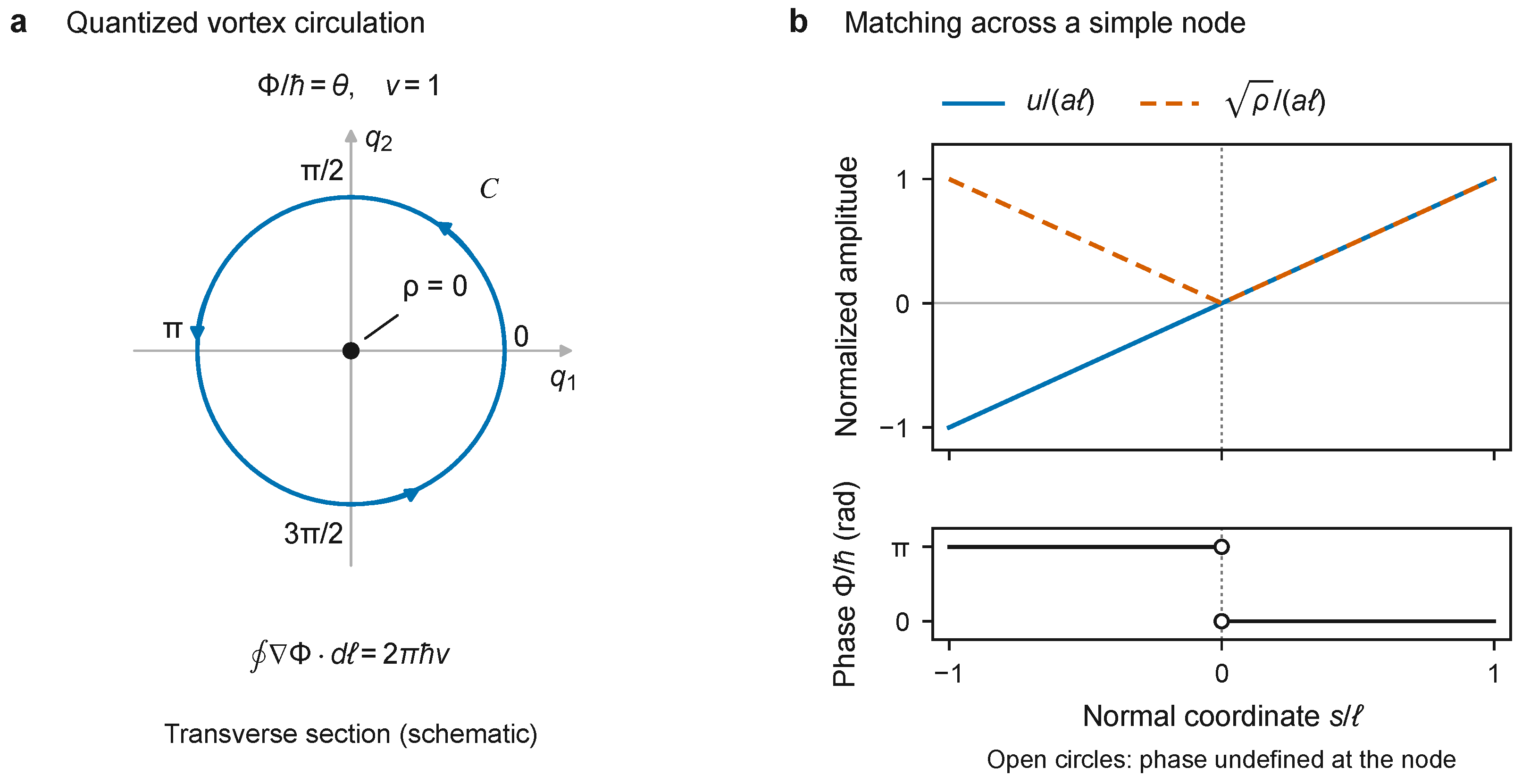
Figure 2.
Dispersive circuit-QED diagnostic rates and synthetic buffered readout. (a) Double-logarithmic memoryless comparison of the source ceiling (blue; illustrative calibration band) and unsaturated SME initial record rate (orange dashed), using Walter et al.’s configuration [41]: , , . Guides mark and . Both rates vanish at , which is omitted on logarithmic axes. (b) Cumulative buffered-budget sweep at : versus . The synthetic parameters are those of panel (c), with varied. Orange shading marks budget excess above ; this parameter set has a distinct memoryless crossover . (c) Deterministic Gaussian-record integration of the synthetic single-mode model for , , , , and . Curves show record mutual information , conditional Holevo storage , their joint cq sum , and cumulative source budget . Constant driving starts from an empty cavity; coupling and drive switch off at (), followed by ring-down. All curves represent synthetic model calculations.
Figure 2.
Dispersive circuit-QED diagnostic rates and synthetic buffered readout. (a) Double-logarithmic memoryless comparison of the source ceiling (blue; illustrative calibration band) and unsaturated SME initial record rate (orange dashed), using Walter et al.’s configuration [41]: , , . Guides mark and . Both rates vanish at , which is omitted on logarithmic axes. (b) Cumulative buffered-budget sweep at : versus . The synthetic parameters are those of panel (c), with varied. Orange shading marks budget excess above ; this parameter set has a distinct memoryless crossover . (c) Deterministic Gaussian-record integration of the synthetic single-mode model for , , , , and . Curves show record mutual information , conditional Holevo storage , their joint cq sum , and cumulative source budget . Constant driving starts from an empty cavity; coupling and drive switch off at (), followed by ring-down. All curves represent synthetic model calculations.
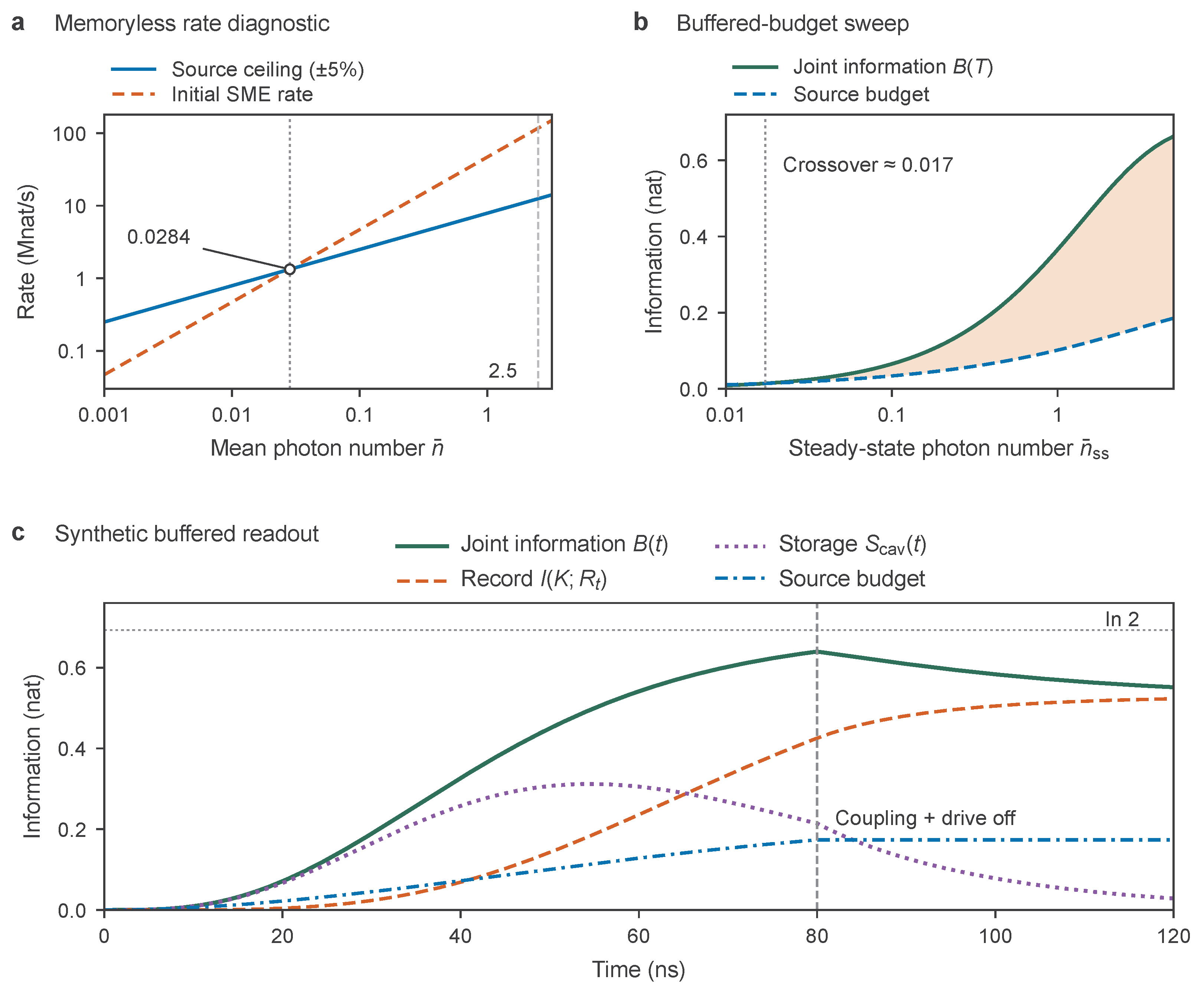

Table 1.
Logical hierarchy and contribution map of the present manuscript.
| Layer | Content in this work | Logical status and closest antecedents |
|---|---|---|
| Inherited structures | Regular-chart Madelung–Kähler geometry (Theorem 1);uncertainty and bound-state spectra (Theorems 3, 6);linear GKSL dynamics (Theorem 7) and local no-signaling (Theorem 8) | Consistency checks and normalization within the density–phase formulation, building on Madelung–Kähler geometry [35,39,40,43], quantum filtering [21,22,24,44], and cQED trajectories [45]. |
| Explicit inputs | Quantized circulation and simple-node matching (Axiom 1);global form domain (Assumption A1);unitary-lift hypothesis (Theorem 2);initial propensities (Postulate 1) | Explicit kinematic, domain, and probabilistic inputs of the formulation. |
| New operational results | Pathwise capacity compatibility (Proposition 5);coherent-pointer Holevo storage budget (Proposition 6) and flat-top posterior drift [Eq. (91)] | Conditional mathematical results: Proposition 6 specializes the general quantum-instrument Holevo inequality [46] to dispersive coherent pointers. The subsequent analysis derives the closed-form flat-top posterior storage drift and examines buffered readout. |
| Empirical hypotheses | Nyquist–Planck bandwidth ceiling (Axiom 2);buffered-channel source budget (Hypothesis 1);laboratory-frame dispersive cQED calibration [Eq. (97)] | Independent, falsifiable hypotheses introduced here. Finite-window budgets test Hypothesis 1 on open damped ports (dynamical completion across remains open); marks the memoryless crossover. |
Table 2.
Canonical laboratory-frame port specification () for dispersive circuit QED.
| Specification element | Operational definition |
|---|---|
| System / environment | Qubit (S, monitored observable ) and readout resonator mode (E, bosonic operator ) in the laboratory frame. |
| Entangling interaction | Dispersive coupling , centered via Eq. (96). |
| Source capacity | for equal-intensity coherent branches . |
| Budgeted information | Joint cq information (record mutual information plus conditional Holevo storage). Hypothesis 1 proposes [Eq. (95)]. |
| Reference state &information set | Conditioned on the receiver’s filtration : (a) coherent superposition (primary ontic test, where is the ontic entangling dispersion of ); (b) receiver-blind random eigenstate preparation ( with prior ), where each shot has zero ontic variance and is evaluated on the receiver-conditioned mixed state via Eq. (96) as an operational communication resource; (c) receiver-known eigenstates (), where and trivially. |
| Independent calibration | (Ramsey/spectroscopy); (resonator ring-down); (ac-Stark shift); (measurement-induced dephasing vs. SNR);dispersive validity requires for qubit–resonator detuning and coupling g [45]. |
Table 3.
Diagnostic readout horizons for the memoryless stationary substitution at [41]. Durations are in nanoseconds with first-order uncertainty propagated from ; is the idealized binary-Gaussian equivalent exposure (dimensionless). The and rows correspond to distinct experimental readout configurations.
Table 3.
Diagnostic readout horizons for the memoryless stationary substitution at [41]. Durations are in nanoseconds with first-order uncertainty propagated from ; is the idealized binary-Gaussian equivalent exposure (dimensionless). The and rows correspond to distinct experimental readout configurations.
| Reported T(ns) | (ns) | (ns) | (ns) | ||
|---|---|---|---|---|---|
| 48 | 1.4114 | ||||
| 88 | 1.7584 |
Disclaimer/Publisher’s Note: The statements, opinions and data contained in all publications are solely those of the individual author(s) and contributor(s) and not of MDPI and/or the editor(s). MDPI and/or the editor(s) disclaim responsibility for any injury to people or property resulting from any ideas, methods, instructions or products referred to in the content. |
© 2026 by the authors. Licensee MDPI, Basel, Switzerland. This article is an open access article distributed under the terms and conditions of the Creative Commons Attribution (CC BY) license (http://creativecommons.org/licenses/by/4.0/).
Copyright: This open access article is published under a Creative Commons CC BY 4.0 license, which permit the free download, distribution, and reuse, provided that the author and preprint are cited in any reuse.