

Submitted:
17 November 2026
Posted:
17 November 2026
You are already at the latest version
Abstract
The debate about the relative importance of interspecific competition and environmental factors in annual population fluctuations has persisted in ecology for many decades. Ecologists face the challenge of determining the extent to which interspecific competition and environmental factors impact population growth rates. We assess the predictive ability of models with and without interspecific competition and environmental covariates to predict population size one year beyond the model-building data. For 11 of 14 datasets a model with interspecific competition and/or environmental factors make better mean ‘absolute’ prediction error. However, none of the models with interspecific competition and/or environmental variables make predictions that are statistically significantly superior to the random walk model. Overall, in about 60% of the sites, models with interspecific competition and environmental variables show performance worse than the random walk baseline model on independent data. We conclude that there is weak evidence that incorporating interspecific competition and/or environmental covariates leads to improved model predictive ability. A thorough assessment of the relative importance of interspecific competition and environmental factors in annual population fluctuations will require evaluating the predictive power of a broader range of models that incorporate ecology of species traits at each generational time.
Keywords:
interspecific competition
; environmental variables
; predictive ability of models
; population dynamics
1. Introduction
Understanding the drivers of population dynamics is essential for developing useful population forecasts and management strategies. The causes of population fluctuations remain one of the unresolved questions in ecological research. Ecological theory suggests that many intrinsic and extrinsic processes such as environmental drivers like temperature or precipitation, or biotic drivers like predators, host-pathogen interactions [1,2], disturbance, intra- or interspecific competition and mutualistic interaction [3,4] can drive population dynamics. Andrewartha and Birch [1] argued that environmental factors are the primary drivers of population fluctuations and more recent ecological research has supported that conclusion [5,6]. By contrast, Nicholson [4] and more recent ecological research asserted that intraspecific [7,8] competition was vital in shaping population abundance by influencing access to limited resources.
Interspecific competition, where different species vie for limited resources needed for growth, survival, and reproduction, can significantly impact population size. Resource scarcity and competition diminishes the availability of resources for other species, potentially resulting in population-level effects [8,9,10]. In addition, environmental factors such as temperature can affect population size through direct impacts on the growth, reproduction, and survival [11]. Warmer temperatures often lead to increased metabolic rates and faster development which results in higher population growth rates during favorable conditions [12]. The effects of temperature may be both direct and indirect through impacts on species interactions [13,14]. Precipitation may also play a pivotal role in the population dynamics of natural population. There exists a positive correlation between precipitation levels and population abundances, suggesting that optimal rainfall patterns can foster larger population sizes. A robust correlation between rainfall patterns and the abundance of African savanna ungulates [15] and rodent populations [16] has been observed. On the other hand, prolonged and irregular fluctuations in precipitation have been associated with diminished growth rates and reduced population sizes [17,18,19]. The debate on the relative importance of interspecific competition and/ or environmental factors on population dynamics has persisted for several decades but has yielded more controversy than clarity. In this paper we address how the integration of interspecific competition and/or environmental factors into ecological models affects our understanding of population fluctuations. Our approach follows on the philosophy that understanding can only be demonstrated by prediction on independent data [20]. Our study will estimate the relative importance of environmental factors and interspecific competition as drivers of population fluctuations by comparing the predictive ability of models with and without interspecific competition and environmental covariates to predict population size one year beyond the data that were used to build the models.
2. Materials and Methods
Dataset selection and procedure: We selected population time series data from 14 different databases (S3 and S4 Tables). These datasets were from multi-sites, multi-year, and multi-species abundance / density databases. 1. We chose only databases with at least 20 consecutive years of surveyed data. 2. We used only population time series from each database with abundance / density greater than zero for each of the years in the time series. We included interspecific competition and environmental variables (temperature, precipitation / Salinity/pH) to investigate the predictive ability of models. Data on environmental variables were extracted from online sources and databases while the interspecific competition index (ICI) was computed using the focal and the competing species (see below for the computation).
Data description: The datasets used in this analysis are from United States (10 out of the 14 datasets), Canada (1 dataset), The Netherlands (2 datasets), and United Kingdom (1 dataset)). The datasets include 3 aquatic ecosystems and 11 terrestrial ecosystems. Types of organisms included birds, plants, zooplankton, rodents, fish, and moths. The number of time series in the datasets ranged from 11 to 7450. The minimum and maximum number of years in a time series is 20 and 30 years respectively. Thus, the maximum number of years in a training set ranged from 11 – 21 years. The mean number of different species in a dataset was around 60 and the range of the number of different species was 3 – 254. Sampling methods included trawl surveys, visual searches, live trapping and quadrat mapping. The units of abundance/density estimates include number of individuals per plot, number of individuals per and percent cover.
Using data to fit models: We fit 4 different functional models to each time series in each of the 14 datasets – ‘Mean’, Trend, Logistic and Gompertz models and used multiple variable combinations for each of the four functional models (see below). The models were fitted to a training set to estimate parameters then the fitted models were used to predict values in the test set.
Interspecific competition: We computed an index representing interspecific competition as follows:
First, we computed the annual growth rate using each species, plots and year
For every Plot × Year combination, we created a matrix to obtain the abundance of every species. For example: if the focal species has abundance; all other species are potential competitors. When Arrowtooth flounder is the focal species, all other species are potential competitors, and then we fit a growth model as follows:
From this equation, we estimated the coefficient () of each competitor j’s abundance on the growth of the focal species i, conditional on other variables. So, the total competition pressure or competition index (CI) was estimated:
This shows that multiply each competitor’s abundance by the estimated coefficients and sum it across the competitors and this finally results in the competition pressure (competition index). If the combined effect of this index is negative, indicating that the competitor effect reduce the focal species growth. Positive competition index shows positive competitor effect on the focal species and zero competition index indicates little or no effect on focal species growth.
Each of the above process was repeated for each species and the following matrix shows that the species on the row side are focal species while the columns indicate the competitor species.
| Species 1 | Species 2 | Species 3 | … | |
| Species 1 | - | α12 | α13 | … |
| Species 2 | α21 | - | α23 | … |
| Species 3 | α31 | α32 | - | … |
| Species 4 | α41 | α42 | α43 | … |
Relative predictive improvement: this shows how well a model predicts as compared to baseline model. We use random walk as a baseline model.
Environmental variables: We extracted the environmental variables from online sources and databases, and we also collected data for some datasets through personal contact with principal investigators (e.g., the pH value for South Central Ontario Zooplankton dataset, environmental data for the Portland rodents and Buell-Small Succession plant survey) (S4 Table). We incorporated the following environmental variables for different ecosystems: temperature and precipitation for terrestrial data, salinity and temperature for marine aquatic systems and pH and temperature for freshwater aquatic systems.
The models: We fit each of the following models and then evaluated model predictive ability. We used precipitation as a covariate for those datasets from terrestrial system (e.g. Hay), for aquatic system we opted to use Salinity (e.g. ALF) and pH (e.g. SCZ) as a covariate.
-
Mean
-
Trend
-
Logistic
-
GompertzWhere: is population abundance at time, is time index, is intercept parameter, are regression coefficients, is random error term at time where , is interspecific competition index at time t and the other environmental variables (temperature, precipitation, salinity and pH) at time t.
The key difference between density independent (Eqs. (1) to Eqs. (10)) and density dependent models (Eqs. (11) to Eqs. (20)) is that the slope in density dependent models is different from zero. Each of the above models was fit to each training set for each time series from each dataset. We fit each of the models above and then evaluated model predictive ability. To allow comparisons to models from our recently published paper in Scientific reports (41) (Table 2), We presented (1) the best model for each dataset from our paper, (2) the random walk model (‘Mean’ model using only the most recent year as training data). (3) the ‘saturated’ model (i.e., the model including all of ICI and the environmental variables) and (4) the best model from models that included at least one of ICI and/or the environmental variables. All these models are extensions of the models used in Scientific Reports (41) and Dennis and Taper (42) classic series of density-dependent papers. For example, for the Aleutian fish (ALF) datasets, the four models are as follows: (1) Gompertz model (41) (2) Random walk model (‘Mean’ model with recent year of training sets). (3) Logistic model with interspecific, salinity, and temperature covariates, and (4) Gompertz model with salinity covariates.
Detailed descriptions of training sets and testing sets: To assess the predictive ability of the population models, the time series data were partitioned into training and testing sets.
Step 1: We selected the last nine years as the test set and the first N-9 years as the training set. Because the number of years in time series ranged from 20-30 years among the datasets, this means that not all training sets across datasets had the same number of years although within each dataset the number of years in each training set was constant.
Step 2: Because we wanted to assess the optimum number of years to include in a training set, we subset the ‘complete’ training set into a series of training sets containing 1, 3, 5…. N-9 years. For example, for a dataset containing time series that were 30 years long, the ‘complete’ training set would include the first 21 years. The ‘complete’ training set would then be subset into training sets of 1,3,5,7,9, 11,13,15,17,19, and 21 years (Fig 3). Subsets would be created by excluding early years. Thus, if a training subset was to only include three years of data, they would be the years 19-21. Data were fit to each of the four models using each of the subsets with the exception of models that could not be fit using a single year (i.e., both density dependent models and the trend model) or year interval (i.e., both density dependent models). In the example for a dataset with 30 years of data, this implies that there would be 10 or 11 sub models (i.e., one for each of the training subsets) for each of the four models.
Step 3: All models were used to predict the year immediately after the last year in the training subset. So, for all subsets of a ‘complete’ training set that included year 21, year 22 would be the predicted population size.
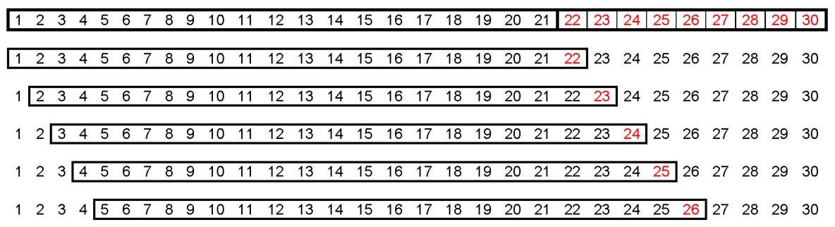
Step 4: “Rolling window”: To maximize the number of predictions available for assessing predictive ability, the training and testing sets were chosen from the time series in a ‘rolling window’ method (Fig 4). This allowed us to compare 5 times as many predicted values to the observed values but still ensures that the model predictions were tested on data that were not used to train the models. The ‘complete’ training set for each database was shifted one year forward in each database and Steps 2-4 repeated. For example, for a database with a 30-year time series that has used years 1-21 for the initial ‘complete’ training set, the training set would be shifted one year forward to include year’s 2-22. This implies that the test set will shrink to eight years in length because there would only be eight years remaining to include in the test set. Now, instead of using models trained on years 1-21 to predict years 22, we used models trained on years 2-22 to predict year 23.
Step 5: We repeated the shift of the ‘complete’ training set forward one year three more times until the available tests set only includes the last five years in the time series. This allowed us to make five replicate predictions for each model/training set combination for each time series in each dataset. For example, for a dataset containing 30 years of data, there were five replicate predictions for the Gompertz model using the 21-year training set to fit a model and predict one year out because we used years 1-21 to predict year 22, years 2-22 to predict year 23, years 3-23 to predict year 24, years 4-24 to predict year 25, and years 5-25 to predict year 26.
Mean prediction error: we calculated absolute prediction error for a single prediction as . Mean prediction error was calculated separately for each model/training set size combination. For example, a dataset containing time series of 30-year duration, would calculate a different mean for the Gompertz with temperature and precipitation covariates 21-year training set, the Gompertz 19-year training, the Gompertz 17-year training set and so on. The mean is calculated across all times series and all 5 replicate predictions for each time series.
where N = number of time series in a dataset (e.g. 968 for Aleutian Island Fish dataset), n = number of replicates for each model/ training set combination (i.e. 5), and prediction error is for a specific replicate of a specific model times series/ training set combination. For example, the Aleutian Islands Fish dataset has 968 time series and there would be 5 replicate predictions for each model/ training set - time series combination for a total of 968 x 5 = 4840 predictions for each Model/ training set combination. That is, the Gompertz model with covariates fit with 19 years in the training set would have 4840 predictions and therefore 4840 prediction errors.
Binomial and Chi-square test for models with and without interspecific competition and/or environmental variables: We conducted a binomial test to examine whether there was a significant difference in the frequency at which models with interspecific competition and/or environmental variables performed best compared to models without these variables. Additionally, we performed a Chi-square test to determine if there was a significant variation in frequency among the four models, which included those incorporating interspecific competition and/or environmental variables, as well as those without them.
Model effects: To test for differences in predictive ability among models, we used generalized linear mixed model (GLMM) with the model term as a fixed effect and site and species as random effects. We used R software for analysis, utilizing lme4 packages for maximum likelihood parameter estimates. For evaluating pairwise differences in generalized linear mixed models (GLMMs), the emmeans package in R was used. This package provides methods for obtaining estimated marginal means and pairwise comparisons. Accordingly, the GLMM was specified assuming a Gamma error distribution with a log link function, which accommodates positive-valued responses and allows the variance to increase with the mean. For statistical comparisons we always compared predictive ability among the four models using the training set size that had the lowest mean prediction error of a particular model. For example, the statistical comparison of the four models for the Aleutian Islands Fish dataset used 17 years of training data for each of the Gompertz, Gompertz with precipitation factors (GompertzPpt) and Logistic including all factors (interspecific competition, temperature and salinity (LogisticICITP), and 5 years for the ‘Mean’ model. This was done separately for each of the 14 datasets.
Prediction error ~ Models + (1|Sites) + (1|Species)
3. Results
3.1. Mean Absolute Prediction Error
Models including one or more of interspecific competition and/or environmental variables gave better predictive ability for 11 datasets (BBSALL birds, BBS10Stop birds, BSS plants, DBBS plants, Hay Plants, Portal rodents (PR), PUSmall plants, PUSquare plants, PUYard plants, Rothamsted Moths (RM), and SCZ zooplankton). Models that did not incorporate environmental variables and interspecific competition still provided the best predictive ability for 3 datasets (AIF fish, Bakker plants, and SNF fish) (Fig 1).
Abbreviations - ‘RW’ represents random walk (mean model trained on a one-year training set), GompertzICITP –Gompertz plus all variables (Interspecific competition, temperature, and precipitation, salinity or pH); GompertzPpt – Gompertz plus precipitation (or salinity/pH); GompertzTemp – Gompertz plus temperature; GompertzICI – Gompertz plus interspecific competition; LogisticICITP – Logistic plus all variables ; LogisticICI– Logistic plus interspecific competition; LogisticPpt – Logistic plus precipitation (or salinity/pH); MeanICITP – Mean model plus all variables; MeanICIP – Mean plus interspecific competition and precipitation (or salinity/pH); MeanICITemp – Mean plus interspecific competition and temperature; MeanPptTemp – Mean plus precipitation and temperature covariates.
The red dashed line in Figure 2 represents the baseline model which is the random walk model. Those models below this red line are underperforming as compared to the baseline model and those above this line are good performing models. In about 60% of the sites, models with interspecific competition and environmental variables shows performance worse than the random walk baseline model on independent data. Similarly, for example, only about for 36% of models with interspecific competition and/or environmental variables in AIF provide significant evidence for model predictive ability (Fig. 2 and S6Table).
Figure 3.
The above grid shows the sliding window approach to get training sets of varying lengths.
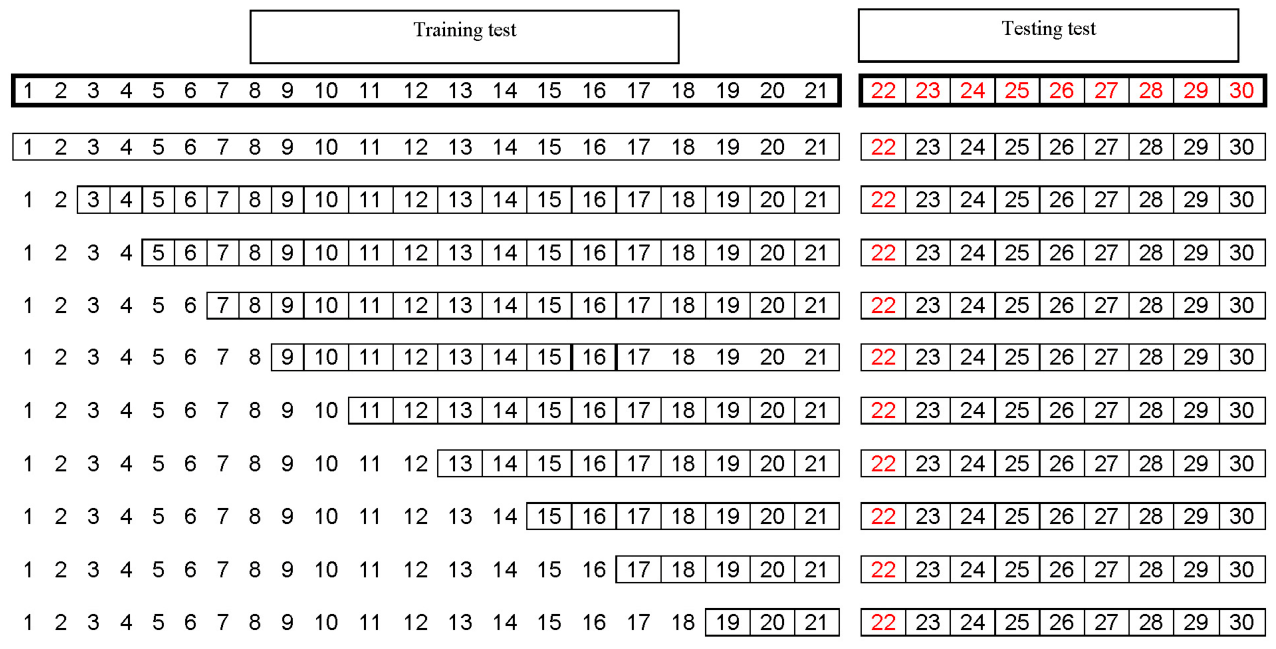
Figure 4.
The grid shows the moving window to get 5 comparisons between observed and predicted values for each training length.
Figure 4.
The grid shows the moving window to get 5 comparisons between observed and predicted values for each training length.
3.2. Statistical Analysis
3.2.1. Binomial and Chi-Square Test for Models With and Without Interspecific Competition and/or Environmental Variables
In 13 of 14 datasets, the most frequent ‘best’ model did not include the interspecific competition index and/or environmental variables (S1 Table). For the only dataset (i.e., BSS) where the most frequent ‘best’ models did include the interspecific competition index and/or environmental variables, it was not statistically significant (the difference in occurrence of best model did not differ between models with and without these variables). Of the 9 datasets where the difference was statistically significant the most frequent ‘best’ model did not include the interspecific competition index and/or environmental variables. The Chi-square test indicated that there was a significant difference in 12 of the 14 datasets among the four models in the frequency that they were the best model (S2 Table) and in all 12 cases the mean or random walk models had the best predictive ability most frequently.
3.3. Generalized Linear Mixed Model
3.3.1. Mean Absolute Prediction Error
For 4 out of 14 datasets, the model term was not statistically significant. For the 10 datasets where the ‘Model’ term was statistically significant, neither of the models with interspecific competition and/or environmental variables was superior to both models without the covariates and/or the random walk model for any dataset (Table 1).
Direction and size of the effect for interspecific competition and/or environmental variables: In 10 out of 14 datasets, the inclusion of interspecific competition had a positive effect on year-to-year changes in abundance of the focal species. For the 3 out of 14 datasets that a model including interspecific competition yielded improved predictive ability, all three showed a positive correlation between the abundance of the focal species and the abundance of non-focal species. Precipitation had a negative effect on year-to-year changes in abundance of focal species population size in 4 out of the 14 datasets while temperature had a positive effect on changes in the population size of the focal species in 6 out of the 14 datasets. For the remaining datasets both precipitation and temperature had negative effects (S5 Table).
4. Discussion
We found that the predictive ability of the ‘best’ population models for the most datasets was weakly improved by adding indices of interspecific competition and/or environmental variables and when including those variables did improve the predictive ability, the improvement was small and not statistically significant. Further, in most cases the presence of interspecific competition index resulted in poor predictive ability of models or, when it improved the predictive ability of models, the effect was small and positive. That is; the more putative competitors there are, the higher the population growth rate [27]. When temperature improved the predictive ability of models the direction of the effect was variable, showing a positive effect in one of the four datasets. Including precipitation only improved predictive ability for one dataset and the effect of precipitation was positive. Salinity and/or pH variables did not help to improve predictive ability in aquatic systems. It was notable that the datasets that showed the strongest evidence of an environmental factor (i.e., temperature) driving population dynamics and no evidence of intra-specific or inter-specific competition were from the Mount St. Helen’s Pumice datasets. These sites were first censused in the year after the Mount St. Helens volcanic explosion and so, are capturing the first thirty years of primary succession.
Effect of interspecific competition: The concept of interspecific competition suggests individuals of different species competing for common resources such as nutrients, water, energy, habitat, and mating opportunities. It has been demonstrated that interspecific competition can play a pivotal role in determining species abundances across various ecosystems. However, it is worth noting that our research did not yield strong evidence to support the idea that interspecific competition drives population dynamics. If interspecific competition was a significant driver of population fluctuation, we would expect to observe a noticeable negative covariance between potential competitors and the focal species [21]. Our results were consistent with Houlahan et al. who found that in more than 50% of populations, there was a positive covariance among species suggesting that interspecific competition is not an important driver of population fluctuations [21]. They concluded that a common response to abiotic factors such as temperature were likely more important than competitive interactions in driving annual population fluctuations. Similarly, Fischer et al. [22] utilized variance ratio and first-order autoregressive models to investigate the driving mechanisms of zooplankton species' population dynamics and concluded that compensatory dynamics are infrequent in communities where species respond similarly to changing environmental conditions. Further, Nowicki et al. [23] concluded that interspecific competition and weather did not have much impact on annual fluctuation of butterfly populations. Adding interspecific competition as a covariate did not seem to improve model predictive performance.
Effect of environmental variables: Environmental variables comprise any abiotic conditions that might influence the survival and reproduction of a species (4) and thus, play a crucial role in shaping the dynamics, distribution, and abundance of species within a particular ecosystem. Weather and climate variables as the drivers of population fluctuation could not be detected [24], but this finding is not consistent with Andrewartha and Birch’s view that environmental variables are the key drivers of population fluctuations (1). They found that a very high proportion of the variance in population density could be explained by environmental factors. Population dynamics of invertebrates are believed to be influenced predominantly by environmental stochasticity [25] and weather patterns are the crucial component of this environmental stochasticity [26]. More generally, the influence of weather on food availability can significantly affect juvenile survival and growth, particularly at high population densities where per capita resource availability is limited [27,28,29].
Environmental effect such as temperature variability influences species populations in a variety of ways, including changing the rates of fundamental processes such as, metabolic rate, photosynthesis, respiration, growth and development and reproduction that determine population size, extinction risk and productivity [13]. Bird communities have shown a positive response to increasing temperature, with some species benefiting from the warming climate and experiencing higher abundances [30]. Temperature-driven range shifts can lead to changes in species abundance in specific regions, as species expand or contract their distributions in response to changing climate conditions [31,32,33]. The investigation of the effect of warming temperature on wetland plant communities showed that increasing temperature led to changes in species abundances, with some species benefiting from enhanced growth and others experiencing reduced abundance [34]. These findings suggested that temperature can have varying impacts on different plant species within a community. However, we observed little evidence in our data that incorporating temperature into population models improved predictive ability.
The dynamic links between climate, water availability and population size may be important. It has been demonstrated that periods of drought and reduced precipitation led to declines in oak tree abundance, while wet periods supported higher population sizes [35]. Further, variations in precipitation levels influenced the abundance and composition of plant species in the grassland [36]. In periods of lower rainfall, some drought tolerant species exhibited enhanced growth and survival while more moisture demanding species experienced a decline in abundance. But we found little evidence that including precipitation in models improved predictive ability.
4.1. Potential Explanations for Weak Predictive Ability of Models Containing Interspecific Competition and/or Environmental Variables
4.1.1. Index of Interspecific Competition
The index we used for representing interspecific competition rarely resulted in improved predictive ability. This might be because interspecific competition has little or no significant impact on the observed population dynamics in these populations. However, one piece of evidence suggesting that this index is unlikely capturing the effects of interspecific competition is that when it did improve the predictive ability of a model, the index was positively correlated with the abundance of the focal species. This is consistent with empirical evidence showing that, in most natural communities, putative competitors co-vary positively [20]. One reasonable explanation for positive covariance is that relatively closely related species (e.g., species in the same family, order, or class) share a common response to environmental changes. Thus, it is plausible that the negative impacts of interspecific competition are obscured by the stronger signal of a common response to the environment. Our study may contribute to the ongoing discussion about suitable indices for capturing interspecific competition effects.
4.1.2. Spatial and Temporal Overlap of Environmental Data
Two key aspects of environmental data are spatial and temporal overlap between focal species abundance and the environmental variables of interest. For most of the datasets, we used data from nearby meteorological stations and assumed that the temperature and precipitation experienced at the station were the same as those experienced by the focal species. We also used the annual mean for both temperature and precipitation, and it is possible, perhaps even likely that temperature and precipitation are only important drivers of population size at specific times of year. The seasonality of environmental variables influences population dynamics [37], but there is relatively limited research specifically addressing the relative importance of seasonality versus annual precipitation [38]. Similarly, temperature fluctuations during critical life stages, such as overwintering or during larval development, affected butterfly population sizes and distribution [39]. So, it is possible that directly measuring temperature and precipitation at each site and identifying the periods of year when temperature and precipitation have the greatest effect on population size would result in temperature and precipitation data increasing the predictive ability of population models.
4.1.3. Measurement Error
Measurement error refers to the discrepancy between the true value of a variable and the value that is observed in a study. Natural animal population sizes are notoriously difficult to estimate, plant abundance may be easier to measure because they are sessile, but there are problems associated with estimating plant abundance as well [40]. It is possible that measurement error on population abundance would be so large that distinguishing the signal from the noise would be difficult.
5. Conclusions
Our findings suggest that there is weak evidence that incorporating interspecific competition and/or environmental covariates leads to improved model predictive ability on independent data. However, these results in line with our previous finding that density-dependent population regulation is rare or weak in natural populations [41], suggest that we must consider that the longstanding scientific belief that population dynamics are driver by density dependence, temperature and precipitation or some combination of the two may be unwarranted. A thorough assessment of the relative importance of interspecific competition and environmental factors in annual population fluctuations will require evaluating the predictive power of a broader range of models that incorporate species ecology traits at each generational stage
Supplementary Materials
The following supporting information can be downloaded at the website of this paper posted on Preprints.org.
Author Contributions
Demissew T. Gebreyohannes carried out the analyses and wrote the first draft of the manuscript and Jeff E. Houlahan conceived the project, made contribution to the analyses and helped with later drafts of the manuscript.
Acknowledgments
This study was supported by NSERC (National Sciences and Engineering Research Council of Canada).
References
- Andrewartha, H.G.; Birch, L. C. The distribution and abundance of animals. In University of Chicago press; 1954. [Google Scholar]
- Lundberg, J.G.; Kottelat, M.; Smith, G.R.; Stiassny, M.L.; Gill, A.C. So many fishes, so little time: an overview of recent ichthyological discovery in continental waters. Ann. Mo. Bot. Gard. 2000, 26–62. [Google Scholar] [CrossRef] [PubMed]
- Mitchell, C.E.; Power, A.G. Release of invasive plants from fungal and viral pathogens. Nature 2003, 421, 625–627. [Google Scholar] [CrossRef] [PubMed]
- Nicholson, A.J. Supplement: the balance of animal populations. J. Anim. Ecol. 1933, 131–178. [Google Scholar] [CrossRef] [PubMed]
- Richardson, D.M.; Allsopp, N.; D’antonio, C.M.; Milton, S.J.; Rejmánek, M. Plant invasions–the role of mutualisms. Bio. Rev. 2000, 75, 65–93. [Google Scholar] [CrossRef]
- Ponciano, J.M.; Taper, M.L.; Dennis, B. Ecological change points: The strength of density dependence and the loss of history. Theo. Pop. Bio. 2018, 121, 45–59. [Google Scholar] [CrossRef] [PubMed]
- Rotella, J.J.; Link, W.A.; Nichols, J.D.; Hadley, G.L.; Garrott, R.A.; Proffitt, K.M. An evaluation of density-dependent and density-independent influences on population growth rates in Weddell seals. Ecology 2009, 90, 975–984. [Google Scholar] [CrossRef] [PubMed]
- Dempster, J. The natural control of populations of butterflies and moths. Bio. Rev. 1983, 58, 461–481. [Google Scholar] [CrossRef]
- Grant, P.R. Interspecific competition among rodents. Ann. Rev. Ecol. Sys. 1972, 3, 79–106. [Google Scholar] [CrossRef]
- Gurevitch, J.; Morrow, L.L.; Wallace, A.; Walsh, J.S. A meta-analysis of competition in field experiments. Am. Nat. 1992, 140, 539–572. [Google Scholar] [CrossRef]
- Holt, R.D.; Lawton, J.H. Apparent competition and enemy-free space in insect host-parasitoid communities. Am. Nat. 1993, 142, 623–645. [Google Scholar] [CrossRef] [PubMed]
- Walther, G.R.; Post, E.; Convey, P.; Menzel, A.; Parmesan, C.; Beebee, T.J.; Fromentin, J.M.; Hoegh-Guldberg, O.; Bairlein, F. Ecological responses to recent climate change. Nature 2002, 416, 389–395. [Google Scholar] [CrossRef] [PubMed]
- Schulte, P.M. The effects of temperature on aerobic metabolism: towards a mechanistic understanding of the responses of ectotherms to a changing environment. J. exp. Bio. 2015, 218, 1856–1866. [Google Scholar] [CrossRef] [PubMed]
- Dee, L.E.; Okamtoto, D.; Gårdmark, A.; Montoya, J.M.; Miller, S.J. Temperature variability alters the stability and thresholds for collapse of interacting species. Philo. Trans. R. Soc. B 2020, 375, 20190457. [Google Scholar] [CrossRef] [PubMed]
- Yu, S.; Song, D.; Fan, M.; Xie, C. Effects of temperature and salinity on growth of Aurelia aurita. Ecol. Model. 2023, 476, 110229. [Google Scholar] [CrossRef]
- Ogutu, J.O.; Piepho, H.P.; Dublin, H.; Bhola, N.R.; Reid, S. Rainfall influences on ungulate population abundance in the Mara-Serengeti ecosystem. J. Anim. Ecol. 2008, 77, 814–829. [Google Scholar] [CrossRef] [PubMed]
- Thibault, K.M.; Ernest, S.M.; White, E.P.; Brown, J.H.; Goheen, J.R. Long-term insights into the influence of precipitation on community dynamics in desert rodents. J. Mammal. 2010, 91, 787–797. [Google Scholar] [CrossRef]
- Drake, J.M. Population effects of increased climate variation. Proc. R. Soc. B Biol. Sci. 2005, 272, 1823–1827. [Google Scholar] [CrossRef] [PubMed]
- Li, G.; Wan, X.; Yin, B.; Wei, W.; Hou, X.; Zhang, X.; Batsuren, E.; Zhao, J.; Huang, S.; Xu, X. Timing outweighs magnitude of rainfall in shaping population dynamics of a small mammal species in steppe grassland. Proc. Natl. Acad. Sci. 2021, 118, e2023691118. [Google Scholar] [CrossRef] [PubMed]
- Zhang, Z.; Xu, L.; Guo, C.; Wang, Y.; Guo, Y. Effect of ENSO-driven precipitation on population irruptions of the Yangtze vole Microtus fortis calamorum in the Dongting Lake region of China. Integr. Zool. 2010, 5, 176–184. [Google Scholar] [CrossRef] [PubMed]
- Houlahan, J.E.; Currie, D.; Cottenie, K.; Cumming, G.; Ernest, S.; Findlay, C.; Fuhlendorf, S.; Gaedke, U.; Legendre, P.; Magnuson, J. Compensatory dynamics are rare in natural ecological communities. Proc. Natl. Acad. Sci. 2007, 104, 3273–3277. [Google Scholar] [CrossRef] [PubMed]
- Fischer, J.M.; Frost, T.M.; Ives, A.R. Compensatory dynamics in zooplankton community responses to acidification: measurement and mechanisms. Ecol. Appl. 2001, 11, 1060–1072. [Google Scholar] [CrossRef]
- Nowicki, P.; Bonelli, S.; Barbero, F.; Balletto, E. Relative importance of density-dependent regulation and environmental stochasticity for butterfly population dynamics. Oecologia 2009, 161, 227–239. [Google Scholar] [CrossRef] [PubMed]
- Knape, J.; De Valpine, P. Effects of weather and climate on the dynamics of animal population time series. Proc. R. Soc. B Biol. Sci. 2011, 278, 985–992. [Google Scholar] [CrossRef] [PubMed]
- Larsson, S.; Ekbom, B.; Björkman, C. Influence of plant quality on pine sawfly population dynamics. Oikos 2000, 89, 440–450. [Google Scholar] [CrossRef]
- Roy, D.; Rothery, P.; Moss, D.; Pollard, E.; Thomas, J. Butterfly numbers and weather: predicting historical trends in abundance and the future effects of climate change. J. Anim. Ecol. 2001, 70, 201–217. [Google Scholar] [CrossRef]
- Hart, E.M.; Gotelli, N.J. The effects of climate change on density-dependent population dynamics of aquatic invertebrates. Oikos 2011, 120, 1227–1234. [Google Scholar] [CrossRef]
- Marino, A.; Pascual, M.; Baldi, R. Ecological drivers of guanaco recruitment: variable carrying capacity and density dependence. Oecologia 2014, 175, 1189–1200. [Google Scholar] [CrossRef] [PubMed]
- Garel, M.; Loison, A.; Gaillard, J.M.; Cugnasse, J.M.; Maillard, D. The effects of a severe drought on mouflon lamb survival. Proc. R. Soc. London. Ser. B Biol. Sci. 2004, 271, S471–S473. [Google Scholar] [CrossRef] [PubMed]
- Devictor, V.; Julliard, R.; Couvet, D.; Jiguet, F. Birds are tracking climate warming, but not fast enough. Proc. R. Soc. B Biol. Sci. 2008, 275, 2743–2748. [Google Scholar] [CrossRef] [PubMed]
- Tingley, M.W.; Beissinger, S.R. Detecting range shifts from historical species occurrences: new perspectives on old data. Trends ecol. evol. 2009, 24, 625–633. [Google Scholar] [CrossRef] [PubMed]
- Chen, I.C.; Hill, J.K.; Ohlemüller, R.; Roy, D.B.; Thomas, C.D. Rapid range shifts of species associated with high levels of climate warming. Science 2011, 333, 1024–1026. [Google Scholar] [CrossRef] [PubMed]
- Sunday, J.M.; Bates, A.E.; Dulvy, N.K. Global analysis of thermal tolerance and latitude in ectotherms. Proc. R. Soc. B Biol. Sci. 2011, 278, 1823–1830. [Google Scholar] [CrossRef] [PubMed]
- Baldwin, H.; Jensen, K.; Schönfeldt, M. Warming increases plant biomass and reduces diversity across continents, latitudes, and species migration scenarios in experimental wetland communities. Glob. Change Biol. 2014, 20, 835–850. [Google Scholar] [CrossRef] [PubMed]
- Mclaughlin, B.C.; Zavaleta, E.S. Predicting species responses to climate change: demography and climate microrefugia in California valley oak (Quercus lobata). Glob. Change boil. 2012, 18, 2301–2312. [Google Scholar] [CrossRef]
- Castillioni, K.; Patten, M.A.; Souza, L. Precipitation effects on grassland plant performance are lessened by hay harvest. Sci. Rep. 2022, 12, 3282. [Google Scholar] [CrossRef] [PubMed]
- Nicolau, P.G.; Ims, R.A.; Sørbye, S.H.; Yoccoz, N.G. Seasonality, density dependence, and spatial population synchrony. Proc. Natl. Acad. Sci. 2022, 119, e2210144119. [Google Scholar] [CrossRef] [PubMed]
- Koenig, W.D.; Knops, J.M. Patterns of annual seed production by northern hemisphere trees: a global perspective. Ame. Nat. 2000, 155, 59–69. [Google Scholar] [CrossRef]
- Parmesan, C.; Yohe, G. A globally coherent fingerprint of climate change impacts across natural systems. Nature 2003, 421, 37–42. [Google Scholar] [CrossRef] [PubMed]
- McComb, B.; Zuckerberg, B.; Vesely, D.; Jordan, C. Monitoring animal populations and their habitats: a practitioner's guide. In CRC Press; 2010. [Google Scholar]
- Gebreyohannes, D.T.; Houlahan, J.E. Weak evidence of density dependent population regulation when using the ability of two simple density dependent models to predict population size. Sci. Rep. 2024, 14, 5051. [Google Scholar] [CrossRef] [PubMed]
- Dennis, B.; Taper, M.L. Density dependence in time series observations of natural populations: estimation and testing. Ecol. Monogr. 1994, 64, 205–224. [Google Scholar] [CrossRef]
Figure 1.
Mean absolute prediction error against number of years of training set size for each of 14 datasets. The symbol 'x' represents the minimum mean prediction error obtained by the best performing model.
Figure 1.
Mean absolute prediction error against number of years of training set size for each of 14 datasets. The symbol 'x' represents the minimum mean prediction error obtained by the best performing model.
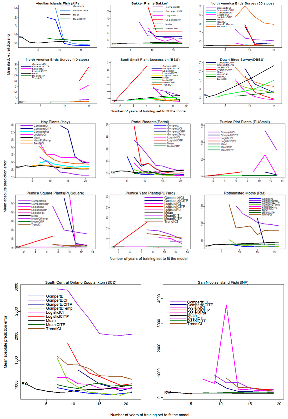
Figure 2.
The relative predictive improvement graph as compared to the baseline (random walk) of the 14 datasets. Abbreviations - GompertzICITP – Gompertz plus all variables (Interspecific competition, temperature, and precipitation, salinity or pH); GompertzPpt – Gompertz plus precipitation (or salinity/pH); GompertzTemp – Gompertz plus temperature; GompertzICI – Gompertz plus interspecific competition; LogisticICITP – Logistic plus all variables ; LogisticICI – Logistic plus interspecific competition; LogisticPpt – Logistic plus precipitation (or salinity/pH); MeanICITP – Mean model plus all variables; MeanICIP – Mean plus interspecific competition and precipitation (or salinity/pH); MeanICITemp – Mean plus interspecific competition and temperature; MeanPptTemp – Mean plus precipitation and temperature covariates. Due to variations in the range of values along the y-axis among the 14 datasets, we grouped datasets with similar y-axis ranges together.
Figure 2.
The relative predictive improvement graph as compared to the baseline (random walk) of the 14 datasets. Abbreviations - GompertzICITP – Gompertz plus all variables (Interspecific competition, temperature, and precipitation, salinity or pH); GompertzPpt – Gompertz plus precipitation (or salinity/pH); GompertzTemp – Gompertz plus temperature; GompertzICI – Gompertz plus interspecific competition; LogisticICITP – Logistic plus all variables ; LogisticICI – Logistic plus interspecific competition; LogisticPpt – Logistic plus precipitation (or salinity/pH); MeanICITP – Mean model plus all variables; MeanICIP – Mean plus interspecific competition and precipitation (or salinity/pH); MeanICITemp – Mean plus interspecific competition and temperature; MeanPptTemp – Mean plus precipitation and temperature covariates. Due to variations in the range of values along the y-axis among the 14 datasets, we grouped datasets with similar y-axis ranges together.
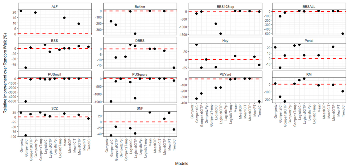

Table 2.
Optimal model for predictive performance across 14 datasets: Insight from the Gebreyohannes and Houlahan (41) Study.
Table 2.
Optimal model for predictive performance across 14 datasets: Insight from the Gebreyohannes and Houlahan (41) Study.
| Datasets | Best model in predictive ability of the 14 datasets from Gebreyohannes and Houlahan’s paper (41) |
|---|---|
| ALF | Gompertz |
| Bakker | Mean |
| BBSALL | Mean |
| BBS10Stop | Mean |
| BSS | Mean |
| DBBS | Mean |
| Hay | Mean |
| Portal | Gompertz |
| PUSmall | Mean |
| PUSquare | Mean |
| PUYard | Mean |
| Rothamsted | Gompertz |
| SCZ | Gompertz |
| SNF | Mean |
Table 1.
Summary of statistical significance of the predictive ability of models for 14 datasets using generalized linear mixed modeling.
Table 1.
Summary of statistical significance of the predictive ability of models for 14 datasets using generalized linear mixed modeling.
| Sites | Models Significance | Pairwise comparison |
|---|---|---|
| ALF | p < 0.05** | NA** |
| Bakker | p < 0.05** | NA** |
| BBSALL | p < 0.001*** | GompertzICITPa MeanPptTempb RandomWalkb |
| BBS10Stop | p < 0.001*** | NA** |
| BSS | p < 0.05** | GompertzICITPb LogisticTempab MeanICIPa RandomWalkab |
| DBBS | p < 0.001*** | GompertzICITPb GompertzTempa MeanICIPa RandomWalkac |
| Hay | p < 0.05** | GompertzICITPa GompertzPptab MeanPptTempb RandomWalkab |
| Portal | p > 0.05 | NA |
| PUSmall | p > 0.05 | NA |
| PUSquare | p > 0.05 | NA |
| PUYard | p < 0.05** | NA** |
| RM | p < 0.05** | Gompertza GpmpertzICITPb GompertzTempab RandomWalkab |
| SCZ | p < 0.05** | NA** |
| SNF | p > 0.05 | NA |
* Models that share the same letters are not statistically significant. NA** in ALF, Bakker, PUYard, and SCZ despite the main effect being significant there were no pairwise comparisons that were statistically significant at the 0.05 threshold.
Disclaimer/Publisher’s Note: The statements, opinions and data contained in all publications are solely those of the individual author(s) and contributor(s) and not of MDPI and/or the editor(s). MDPI and/or the editor(s) disclaim responsibility for any injury to people or property resulting from any ideas, methods, instructions or products referred to in the content. |
© 2026 by the authors. Licensee MDPI, Basel, Switzerland. This article is an open access article distributed under the terms and conditions of the Creative Commons Attribution (CC BY) license (http://creativecommons.org/licenses/by/4.0/).
Copyright: This open access article is published under a Creative Commons CC BY 4.0 license, which permit the free download, distribution, and reuse, provided that the author and preprint are cited in any reuse.