

Submitted:
13 November 2026
Posted:
16 November 2026
You are already at the latest version
Abstract
Off-grid microgrids have emerged as an attractive solution for rural electrification in
Southern Africa, particularly for farms and remote communities where extending the
utility grid is costly and grid supply is unreliable. However, the high capital cost and short
lifespan of battery energy storage systems (BESSs), compared to microgrid components
such as PV modules and inverters, remain financial barriers. Since BESS replacement
represents a major lifecycle cost, extending battery lifespan can improve the economic
viability of off-grid microgrids. This paper proposes a SOH-aware energy management
system (EMS) for off-grid microgrids. The proposed EMS combines a hybrid battery
degradation model, which couples data-driven and physics-based methods, with model
predictive control (MPC) to optimise battery usage while maintaining system reliability.
The proposed EMS is validated by hardware-in-the-loop (HIL) simulation on an OPAL-
RT OP4512 real-time simulator. Compared with a conventional rule-based EMS, the
proposed EMS reduces modelled battery capacity fade by 67% at 100% state of health
(SOH) and by 61% at 82% SOH. Compared with a tuned rule-based EMS, the
reductions are approximately 11% and 12% at the same two SOH levels, which shows
that the proposed EMS reduces degradation beyond what lowering the SOC ceiling of a
rule-based EMS achieves.
Keywords:
battery energy storage systems
; degradation
; energy management system
; hardware-in-the-loop simulation
; microgrids
; model predictive control
1. Introduction
As the world continues to transition towards sustainability, microgrids have emerged as one of the premier sustainable energy solutions [1]. Microgrids provide a platform to reduce dependence on fossil fuels by generating electricity from renewable energy sources close to the point of consumption and using energy storage and coordinated control to manage renewable generation variability [2]. Microgrids also offer localized control over energy distribution and serve as an interface to connect energy produced from renewable energy sources to the traditional grid or as a medium for local renewable energy consumption without grid connection, in stand-alone mode [3]. In southern Africa, stand-alone microgrids have been deployed primarily in remote areas to support rural electrification [4]. An example of such an application of off-grid microgrids can be found in Ventersdorp, South Africa, where a 200 kWp off-grid microgrid is used as the main power source for farm operations and the local farm community. The PV system is backed up by 500 kWh of battery energy storage for overnight loads and during periods of low solar production. Such systems prove to be attractive solutions for rural electrification, particularly in remote locations where extending the conventional electricity grid is not economically feasible. Although the initial capital investment in microgrid infrastructure can be substantial, the long-term benefits of eliminating utility tariffs, improved energy independence and avoided grid extension costs can justify the investment in off-grid microgrids [5].
However, despite their potential long-term economic benefits, the initial capital investment associated with off-grid microgrid components particularly battery energy storage systems (BESSs), poses a significant barrier for adoption of off-grid microgrids [6]. Furthermore, the relatively short lifespan of BESS compared to other microgrid components, such as solar photovoltaic (PV) panels and inverters, introduces an additional financial challenge, as BESSs may require replacement several times throughout the operational lifetime of the microgrid. These replacement costs increase the overall lifecycle expenditure and can significantly undermine the long-term economic viability of off-grid microgrids, particularly in rural communities where access to capital is limited [7].
The operational lifespan of a BESS is influenced not only by its battery chemistry and design, but also by operating conditions such as the state of charge (SOC), depth of discharge, charging and discharging rates, and temperature [8]. These operating conditions contribute to battery degradation, which is characterised by the gradual and permanent reduction in the BESS’s ability to store and deliver energy [9]. Since microgrid energy management systems (EMSs) govern the charging and discharging behaviour of BESSs, they play a critical role in determining the rate at which BESSs’ degradation occurs [10]. Conventional microgrid energy management strategies primarily focus on maintaining the balance between energy generation and consumption while ensuring that the BESS operates within predefined limits [11]. However, these strategies do not necessarily account for the progressive deterioration of battery health when making energy dispatch decisions [12]. This highlights the need for more advanced energy management strategies that incorporate battery state of health (SOH) information into the decision-making process. By adapting charging and discharging decisions according to the battery’s health condition, SOH-aware energy management systems have the potential to minimise battery degradation, extend its operational lifespan and ultimately improve the long-term economic viability of off-grid microgrids [12].
EMSs are essential for coordinating power generation, BESSs and load demand in off-grid microgrids [13]. Rule-based energy management strategies are among the simplest and most widely adopted approaches, owing to their straightforward implementation, low computational requirements and ability to maintain power balance using predefined operating conditions [14]. Safder et al. [15], demonstrate the effectiveness of a rule-based EMS (RB-EMS) in a standalone DC microgrid comprising photovoltaic generation, BESS and fuel cells, achieving coordinated power sharing and DC bus voltage regulation under varying operating conditions. Their proposed EMS prioritises PV generation, followed by battery storage and fuel cells, while maintaining the battery SOC between 20% and 80% to prevent excessive charging and discharging. Simulation and experimental validation demonstrated that the EMS maintained the DC bus voltage at approximately 380 V, with fluctuations within 4% of the nominal voltage, although the strategy did not explicitly account for battery SOH or degradation when determining dispatch decisions.
However, conventional rule-based approaches are generally reactive, with limited ability to anticipate future variations in generation and demand or optimise system operation beyond predefined control rules [16]. To overcome these limitations, researchers have investigated more sophisticated strategies, including fuzzy logic control, mathematical optimisation and artificial intelligence-based techniques in off-grid microgrid applications [17,18,19,20,21]. Fuzzy logic EMSs offer greater flexibility in managing uncertain operating conditions by determining control actions through membership functions and linguistic rules rather than rigid operating thresholds [22].
Optimisation-based EMSs, including linear programming, mixed-integer programming and metaheuristic algorithms, have also been extensively investigated to determine suitable power dispatch schedules while minimising operating costs, fuel consumption and other performance objectives [23]. More advanced approaches employ model predictive control (MPC) strategies, which typically use system models and forecasts to optimise control decisions over a finite prediction horizon while explicitly incorporating operational constraints. Polimeni et al. [24] developed and experimentally validated a hierarchical stochastic MPC-based EMS for an off-grid microgrid, demonstrating improved economic performance through the consideration of forecast uncertainty. Similarly, Salazar et al. [25] proposed an MPC-based EMS for an isolated microgrid in the Ecuadorian Amazon, incorporating battery degradation and SOH considerations to improve long-term system operation. More recently, intelligent approaches employing machine learning and reinforcement learning have attracted increasing attention due to their potential to adapt energy management decisions to complex and uncertain operating conditions [26]. Despite these developments, advanced EMSs introduce additional modelling, computational and implementation requirements, while the integration of reliable online battery health estimates into real-time dispatch remains an important area of investigation, particularly for off-grid microgrids where battery longevity and reliable electricity supply are critical.
BESS SOH-aware energy management strategies for lithium-ion batteries have been studied extensively in literature [27,28,29,30,31,32,33]. The existing body of work generally accounts for degradation by incorporating simplified degradation cost models or penalty functions into energy management system (EMS) objective functions [27]. Factors such as depth of discharge (DOD), charging and discharging rate (C-rate) and operating temperature are used to assign the associated ageing cost. Others account for degradation by counting complete and incomplete battery cycles using the rainflow method as used in [28,29]. In [30], battery degradation is considered in predictive energy management. The approach involves a non-linear degradation model that only incorporates cycle ageing into the capacity fade model, excluding calendar fade, a significant weakness in the approach. Terkes et al. [31] go further on the approach from Guo et al. [30], by incorporating both cycle ageing and calendar ageing in their capacity fade model. The authors propose a novel multistage, multi-objective optimisation algorithm that considers battery degradation and life cycle cost minimisation developed for battery control strategies. Cycle fade is modelled as a throughput-based quantity, normalised by DOD-dependent cycle life and twice the fresh capacity, whilst calendar fade is modelled as a linear curve fit. The two are then coupled, ensuring that capacity fade shrinks the operating envelope of the objective function, not just the objective value. Their results show that their proposed method reduces BESS lifecycle cost by up to 18.4%. However, a weakness of this approach is that calendar ageing is modelled as a linear function of battery power. The model, therefore, does not account for the growth in internal resistance as the battery ages and thus fails to capture the associated power fade.
In [32], the authors introduce a novel predictive energy management strategy to integrate the degradation cost of lithium-ion BESS into the optimal dispatch of a grid-connected PV-BESS system. The proposed approach models both calendar and cycle ageing, with calendar ageing represented as a function of SOC and cycle ageing determined according to the depth of discharge of complete and incomplete cycles. A linear degradation-cost function is then developed using the estimated capacity fade and relevant financial parameters, allowing the degradation cost to be incorporated directly into the optimisation problem. A model predictive control (MPC) based predictive energy management systems (PEMS) is subsequently used to determine the BESS charge/discharge schedule while accounting for forecasted PV generation and real-time electricity prices. Simulation results demonstrate that incorporating degradation into the energy management strategy influences the BESS operating schedule and can reduce capacity fade and degradation cost. Compared with a conventional scheduling strategy, the proposed PEMS reduced capacity fade by 5.06% and degradation cost by 4.67%, while increasing PV-farm profit by 1.10%.
Collectively, these studies demonstrate a progression from explicitly incorporating modelled degradation costs into conventional optimisation frameworks towards adaptive learning-based EMS approaches; however, most studies still majorly rely on linear capacity fade models, equivalent degradation costs, or offline battery ageing models rather than continuously estimating the actual health condition of the battery during operation. Consequently, changes in battery state of health (SOH), internal resistance, available capacity, and degradation rate are often not explicitly incorporated into the real-time dispatch decision, which motivates the approach adopted in this paper.
To account for BESS degradation in microgrid energy management, it is important to understand how battery SOH changes during microgrid operation [8]. State of health (SOH) quantifies the current condition of a battery relative to its rated condition when it is brand new [33]. Remaining useful life estimation (RUL) takes SOH as input and outputs a prediction of the residual life of the battery [34,35]. Battery state cannot be directly measured but rather inferred from its external behaviour [36]. Several approaches to estimating SOH and RUL have been proposed in literature and they can generally be classified into model-based methods, data-based methods and hybrid methods [37].
Physics-based models, such as the state estimation method used by Wang et al. in [38], are simplified, computationally efficient approaches for predicting the future behaviour of battery cells. However, they often suffer from cumulative prediction errors that result from the inability to account for the coupled electrochemical, thermal, and mechanical ageing mechanisms. This reduces their reliability for long-term degradation forecasting as a result [39]. Conversely, data-driven approaches offer strong long-term predictive capability but often lack physical interpretability and require large datasets for reliable performance [40]. Hybrid approaches have therefore emerged as a promising alternative, combining physical knowledge with data-driven learning to improve the accuracy, robustness and interpretability of battery health estimation [41].
Lyu et al. [42] propose a hybrid model–data fusion framework for simultaneous SOH estimation and RUL prediction of lithium-ion batteries. Their approach combines a metabolic grey model (MGM) and multiple-output Gaussian process regression (MOGPR) to model nonlinear battery capacity degradation, using resistance parameters derived from a Thévenin equivalent circuit model (ECM) as ageing indicators. A particle filter is subsequently employed to update the estimated degradation states using battery measurements and predict the remaining useful life. The authors demonstrate the effectiveness of the framework under different temperature conditions, highlighting the benefits of combining physical ageing indicators with statistical degradation modelling and probabilistic state estimation. Building on the advantages of incorporating physical information into data-driven estimation, Wang et al. [38] develop a model–data fusion approach using battery-model-derived health indicators and domain adaptation to improve SOH estimation under varying operating conditions. Their method demonstrates that physically informed features can improve estimation accuracy while reducing the amount of training data required for application to different battery operating conditions.
Further developments in probabilistic hybrid estimation are presented by Lyu et al. [43], who propose a data-fusion-model framework combining dual Gaussian Process Regression models with a rejection-sampling particle filter. The Gaussian Process Regression models characterise nonlinear battery ageing behaviour using charging-derived health indicators, while the particle filter improves the tracking of battery degradation under measurement uncertainty. The study demonstrates improved SOH estimation performance compared with conventional estimation methods, reinforcing the value of probabilistic filtering in hybrid battery health estimation. However, accurate battery health estimation alone does not necessarily translate into reduced battery degradation unless the estimated health information is incorporated into operational decision-making. This highlights an opportunity to extend hybrid SOH and RUL estimation frameworks beyond battery health monitoring into degradation-aware energy management, where battery health estimates can be used to adapt charging and discharging constraints as the battery ages.
This paper therefore presents an SOH-conscious model predictive control (MPC), energy management system (EMS) for off-grid microgrids. The proposed approach integrates a second-order Thévenin equivalent circuit model (ECM) with a hybrid physics–data battery health estimation framework incorporating a Metabolic Grey Model (MGM), Multi-Output Gaussian Process Regression (MOGPR), and particle filtering, drawing on the work of Lyu et al. The framework provides SOH estimates to the MPC, which incorporates an SOH-dependent charging C-rate limit as an explicit operational constraint rather than treating battery degradation solely as a penalty in the optimisation objective function. This establishes a health-dependent feasible operating region that progressively contracts as the battery ages, allowing the EMS to adapt its charging decisions to the battery’s declining health. On a modelled 500 kWh LFP BESS at SOH 0.82, the controller reduces capacity fade from 0.0150%/day under a stock rule-based baseline to 0.0058%/day, with 100% load service. The EMS is validated in real time on an OPAL-RT OP4512, executing a full day closed-loop at 1440 control steps with no deadline misses, demonstrating real time feasibility.
The rest of this paper is organised as follows. Section 2 models the microgrid and its BESS, and Section 3 presents the health estimator. Section 4 formulates the SOH-aware MPC and the rule-based baselines. Section 5 presents and discusses the results, including the hardware-in-the-loop validation and a comparison with previous studies, and Section 6 concludes the paper.
2. Microgrid Modelling
2.1. Microgrid Plant Model
The proposed SOH-aware energy management framework is evaluated on a microgrid platform consisting of PV generation, power conversion systems and a BESS. The PV production is based on established PV performance models, the NREL PVWatts model and the Nominal Operating Cell Temperature (NOCT) models from [44,45]. PV generation is therefore modelled as a bell-shaped irradiance curve which incorporates temperature derate and cloud cover events to simulate cloud cover. Mathematically, PV generation is given as,
where PDC is the DC power generated from the PV modules, Ppeak is the maximum possible PV production based on the capacity of the PV modules, g is the normalised irradiance, γ is the PV power temperature coefficient and cc is the cloud cover factor. Tcell, the average cell temperature of the PV cells is given as,
where Tamb is the ambient temperature and NOCT is the Nominal Operating Cell Temperature provided by the PV panel manufacturer. Inverters handle the power conversion from DC to AC and vice versa. The inverters are wired in an AC-coupled architecture where the output of a dedicated power conversion system (PCS) inverter for the battery is coupled with the output from a dedicated PV inverter as given in Figure 1. The split AC architecture decouples the sizing of the PV and storage subsystems allowing for future expansion of the PV array, or replacement of the battery modules at end of life, without re-engineering a shared DC voltage window and providing redundancy in the event of failure of one of the inverters. Mathematically the power from each PV inverter in kW PPV is given as,
where ηPV is the inverter efficiency as provided by the manufacturer, PDC is the DC power generated by the PV array in kW and PPV,rated is the maximum rated AC output of the PV inverter in kW. The minimisation function, therefore, ensures that the inverter output never exceeds its rated AC power capacity. When sufficient DC power is available, the inverter reaches its rated AC output, however, if DC power exceeds the inverter capacity, the output is clipped, that is
Unlike the PV inverter, which primarily converts DC power into AC power, the BESS PCS is bidirectional. The PCS is represented using a simplified steady-state model that accounts for bidirectional conversion efficiency and rated power limitations. Similar efficiency-based representations of battery power conversion systems are employed in the NREL System Advisor Model (SAM) for evaluating battery storage performance [46]. The model is therefore represented as,
where PPCS,max is the maximum rated active power of the PCS inverter in kW, PBESS,DC is the DC power delivered by the BESS to the PCS inverter for conversion, PBESS,AC is the AC power delivered by the BESS through the PCS to the loads in kW and ηPCS is the conversion efficiency of the inverter as provided by the manufacturer. PBESS,AC is positive during discharging and negative during charging. The microgrid is islanded; no utility connection is present. Therefore, at any point in time (k), the load must be supplied by either PV power, BESS energy or a combination of both as,
where Pload(k) represents power in kW supplied to the load at time step k. PBESS,AC(k) is positive when the battery discharges and negative when it charges. The load model is based on logged data at a case study site in Ventersdorp in South Africa. Two weeks’ worth of logging data is extrapolated over a year and the typical daily load is used when simulating the microgrid power flow. The resultant load profile is shown in Section 5.
2.2. Microgrid BESS Mathematical Model
The performance of the proposed energy management system depends on an appropriate representation of the electrical behaviour of the BESS under different charging and discharging conditions. Although the EMS determines battery power commands at the control level, the resulting battery current, terminal voltage and state of charge depend on the electrical characteristics of the BESS. Consequently, an electrical BESS model is required to represent the response of the BESS to the dispatch decisions generated by the proposed EMS. The BESS electrical model also provides a framework for incorporating the electrical consequences of battery ageing into the microgrid plant model. As the battery degrades, its available capacity decreases, while changes in internal resistance can influence terminal voltage and electrical losses. In this research, a Thévenin ECM consisting of an open-circuit voltage source VOCV, a series ohmic resistance R0, and two parallel RC branches is used to represent the microgrid BESS. The model is based on a similar approach adopted by Bian and Ma [47], and it consists of an open-circuit voltage source, an ohmic resistance and two resistor-capacitor (RC) networks that approximate the transient polarisation behaviour of the BESS. Compared to an ideal battery representation, the ECM captures the influence of internal resistance and dynamic voltage response during charging and discharging. The second-order configuration is selected as a compromise between the ability to capture both fast and slow changes in battery voltage and the computational requirements associated with numerical simulation. A representation of the Thévenin circuit model is given in Figure 2.
Taking battery current as positive during discharge and negative during charging, from Figure 2, the terminal voltage is given by Kirchhoff’s voltage law (KVL) and expressed as,
where Vt(k) is the pack terminal voltage, I(k) is the battery current, and VRC1(k) and VRC2(k) are the polarisation voltages associated with the two RC branches. The continuous-time dynamics of the two RC branches can be written as,
and
The associated time constants are therefore given as,
The state of charge (SOC) is calculated by Coulomb counting. However, rather than assuming that the nominal ampere-hour capacity remains constant throughout battery life, the present effective capacity Qeff(k) is related to SOH as
where Qnom is the beginning-of-life nominal capacity and SOH(k) is the capacity-based state of health expressed as a fraction of the nominal pack capacity.
Taking discharge current as positive, sampling at ∆t intervals in seconds, the state of charge expressed as a fraction from 0 to 1, updates as,
where SOC(k) is the battery SOC at time step k, expressed as a fraction from 0 to 1, i(k) is the pack current in amperes (positive during discharge), Qnom is the nominal pack capacity. The factor 3600 converts ampere-seconds to ampere-hours.
2.3. Ageing Dataset and ECM Parameter Identification
The parameters of the second-order Thévenin ECM are identified using hybrid pulse power characterisation (HPPC) data from the BAK N18650CL-29 cylindrical lithium-ion cell from a MathWorks dataset. The identified parameters are presented in Table 1. HPPC, extensively used in literature [48,49], applies several discharge–charge pulse pairs, each followed by a constant-current step that lowers the state of charge by approximately 10%, with a one-hour rest after every pulse sequence so the RC branch voltages decay fully before the next measurement. Ohmic resistance is taken from the instantaneous voltage step at pulse onset and offset, where the current transition excites it directly. In addition to the MathWorks BAK dataset, ageing data from NASA Ames Prognostics Center of Excellence (PCoE) Data Repository, in particular cells B0005, B0006, B0007 and B0018 are used for SOH modelling as described in Section 3.2. The dual dataset approach allows for circuit parameters and ageing trajectory to be extracted from pulse characterisation data and run to failure cycling data, respectively, overcoming the limitations of publicly available datasets that do not adequately support both objectives.
The Thévenin ECM parameters in Table 1 are obtained from individual lithium-ion cells, whereas the microgrid considered in this study employs a BESS at a significantly larger scale. Ideally, the ECM parameters of the BESS would be identified directly from HPPC tests conducted on the battery modules or packs used at microgrid scale. However, such experimental data are not readily available. Consequently, an alternative approach is adopted from literature [50], in which ECM parameters identified at the cell level are scaled to represent the electrical characteristics of the larger BESS. This approach provides a practical means of developing a pack-level electrical model in the absence of direct experimental data, although it relies on simplifying assumptions regarding cell uniformity and pack configuration. This section therefore presents the methodology used to scale the cell-level parameters to the microgrid BESS level.
Under the assumption of identical cells operating under uniform conditions, the scaling preserves the characteristic RC time constants of the cell-level ECM. The resulting scaling relationships are given as,
and
where Ns and Np represent the number of cells in series and parallel in a battery pack respectively. Vpack and Qpack are the BESS pack voltage and capacity in volts and ampere-hours, respectively. Vcell is the cell voltage and Qcell is the cell capacity in ampere-hours. The nominal pack energy (Epack) is then given as,
The resistance circuit parameters () are scaled from cell to pack level as given,
where Rpack and Rcell represent pack and cell level resistance respectively. Similarly, the capacitances (C1,C2) associated with the RC branches exhibit the inverse scaling relationship given as,
where Cpack and Ccell represent pack and cell level capacitance respectively.
However, the time constants of both RC branches remain unchanged when transitioning from cell to pack level as shown,
Parameter scaling preserves the dynamic response characteristics of the individual-cell Thévenin ECM while scaling its electrical magnitude to represent the complete battery pack. The open-circuit voltage is scaled differently because cells connected in series contribute directly to the total pack voltage. In addition to the ideal cell scaling, a fixed pack-level interconnection resistance is included to represent resistive contributions from busbars, welds, contactors, and cabling. Unlike the cell-derived resistance, this component is treated as a series resistance at pack level and is therefore not scaled according to Ns/Np.
3. BESS Health Estimation
3.1. Capacity Fade Evaluation Model
To accurately predict the evolution of BESS health throughout its operational lifetime, it is essential to develop a mathematical model that adequately captures the underlying capacity degradation mechanisms. In this paper, therefore, degradation is represented by a semi-empirical model that separates calendar from cycle ageing. The model is a semi-empirical formulation combining calendar and cycling ageing contributions that combines approaches from [31,32]. The total modelled capacity loss over an evaluated period is calculated as,
where ΔQtot represents the total capacity loss, ΔQcal represents calendar-related capacity loss and ΔQcyc represents cycling-related capacity loss. Calendar degradation is represented as a time-dependent capacity-loss rate that increases exponentially with SOC. At each simulation step, the calendar-ageing contribution is calculated as,
where kcal is the reference calendar-ageing coefficient expressed in percentage capacity loss per day, kSOC defines the sensitivity of calendar ageing to SOC, SOC(k) is the battery SOC at time step k, and Δt is the simulation time step in seconds. The accumulated cycle-ageing contribution is expressed as,
where kcyc is the reference capacity loss per equivalent full cycle, kC increases the cycling penalty at higher C-rates and ΔEFC(k) is the equivalent full-cycle increment at time step k, given as,
3.2. SOH and RUL Estimation
This paper adopts the use of a hybrid MGM, MOGPR and a particle filter as used by Lyu et al. [42], to estimate battery state of health and predict the remaining useful life of the microgrid BESS. The health estimator is trained and tested on four cells of the NASA PCoE ageing dataset. Cells B0005 and B0006 are used for training, and B0007 and B0018 are held out for testing, so no test-cell data is used in training or tuning. Training, in this context, refers to the process in which a model learns the degradation trend from the measured data of selected cells, by adjusting its internal settings until its predictions match those measurements. Testing, on the other hand, means comparing the SOH degradation trajectories predicted by a model against the actual degradation trajectories obtained from the NASA dataset. For every cell, health is defined from the per-cycle discharge capacity as shown,
and
where k is the cycle number, Qk is the measured discharge capacity at cycle k (Ah), Qnom is the beginning-of-life reference capacity of the cell (Ah), and QEOL is the end-of-life (EOL) capacity. The threshold of 80% SOH is adopted in this research as the criterion for EOL because this threshold is widely used in lithium-ion battery degradation studies as a conventional benchmark for evaluating battery lifetime and RUL [51,52]. The MGM provides a cell-specific capacity observation from measured data alone. The MOGPR provides the population ageing trend learned from the training cells. The particle filter fuses the two into SOH and RUL estimates with credible intervals. Table 2 lists the settings. The following sections describe the mathematical model of each of the MGM, MOGPR and the particle filter.
3.2.1. Stage 1: MGM Observation
At each cycle k > W, a first-order grey model, GM(1,1), is fitted to the W = 5 most recent measured capacities, q(0)(m) = Qk−W−1+m for m = 1,…,W. The model is called metabolic because the window rolls: each new measurement enters the window and the oldest leaves. The accumulated sequence and its background values are given as,
and
where q(1)(m) is the capacity accumulated up to the mth window entry and , for m = 2,…,W, is the mean of two consecutive accumulated values. The development coefficient a and grey input b of the grey equation are found by least squares as
and
where holds the window capacities from the second entry onwards. Solving the whitened equation and differencing its accumulated response gives the one-step-ahead estimate of the current capacity as shown,
The MGM fit can predict a rise in capacity, for example when a regeneration jump falls inside the window, yet capacity cannot recover through ageing. The estimate is therefore limited to no more than the last measured capacity and no less than zero. The result is the output of Stage 1, the capacity observation that the particle filter in Stage 3 uses to weight its particles, given as,
where zk is the MGM observation at cycle k (Ah). For the first W cycles, zk = Qk.
The observation noise is set from the MGM residuals of the training cells only, rk = zk − Qk for k > W. The NASA cells show capacity regeneration: measured capacity rises after a rest period while the clamp holds zk flat. This gives the residuals a long one-sided tail that reflects a known electrochemical effect rather than observation noise. A robust scale is therefore used, given as
where med(r) is the median over the pooled training residuals, 1.4826 scales the median absolute deviation to the standard deviation of a Gaussian, and 0.005 Ah is a lower bound. This gives σz = 0.0087 Ah. Because the residuals are heavy-tailed, the likelihood in Stage 3 is a student-t density with scale σz. Its degrees of freedom, ν, are fitted by maximum likelihood to the same residuals.
3.2.2. Stage 2: MOGPR
The MOGPR takes the cycle number x = k as its input and has two outputs y1 and y2 given as,
and
where Rapp is the apparent resistance obtained from the voltage step at the start of discharge, and Rapp,fresh is its mean over the first three cycles of the cell. Both outputs are relative to the cell’s own fresh values, so cell-to-cell spread in fresh capacity is removed before training. Each output is then standardised with the training mean and standard deviation. The two outputs share one squared-exponential kernel given as,
where is the length scale in cycles, (x,x') are two input points, and is the signal variance. The outputs are coupled through the intrinsic coregionalisation model (ICM):
and
where i,j ∈ {1,2} index the outputs and Bij is element (i,j) of the 2 × 2 coregionalisation matrix B. holds the loadings of the two outputs on a shared latent trend, and holds positive output-specific variances. B is positive semidefinite by construction and carries the signal variance, so the kernel has no separate amplitude. The learned correlation coefficient ρ is the learned cross output correlation. It shows how strongly the learned SOH trajectory and normalised resistance trajectory are statistically coupled. This is particularly meaningful physically because battery degradation generally involves both capacity fade, and internal-resistance growth. The strength of the learned coupling ρ is given as,
where a negative ρ means that W1 and W2 have opposite sign, so the SOH falls as the normalised resistance rises. For a test cell, only its cycle numbers and Qnom are used. The SOH prediction is converted back from standardised units into a prior capacity path as shown,
and
where is the capacity (Ah) that the population trend predicts for the test cell at cycle k, is the standard deviation of that prediction. and d1 are the training mean and standard deviation of the SOH output. Beyond the cell’s last recorded cycle, the path is extended linearly at its final 20-cycle slope, with a magnitude of at least half the mean training fade rate defined in Stage 3. The particle filter uses the increments of this path. They are clamped so that the population trend never gains capacity, as
3.2.3. Stage 3: Particle Filter
Each of Npf = 500 particles, i = 1,…,Npf, carries a capacity (Ah) and a degradation-speed factor . The speed factor scales the population trend to the cell being tracked: s = 1 means the cell ages at the population rate, and s < 1 means it ages more slowly. At the first cycle, and . Here σs,0 = max(0.25, std(sc)) is the spread of the speed factors of the two training cells,
where Dc is the SOH drop of training cell c over their common record length and is the mean of the two drops. The lower bound of 0.25 is used because two cells form a small sample.
The speed factor is a fixed property of the cell, and it is propagated as shown,
where and are the weighted mean and variance of the speed factors, and is the normalised weight of particle i. is a standard normal draw. The shrinkage λ is given as
and kernel width h given as,
follow from the discount factor δ=0.98, giving λ = 0.990 and h = 0.142. Each is limited to [0.2, 3.0]. The capacity follows the population increment, scaled by the particle’s own speed factor, as
where is the process noise (Ah). Each is limited to [0, 1.05 Qnom]. The per-cycle noise σproc is given by
where is the mean fade rate of the training cells, given as
where Qc,1 and are the first and last capacities of training cell c and Kc is its number of cycles.
The weights are updated with the student-t likelihood of the MGM observation, given as
The effective sample size, Neff is given as
and when it falls below Npf/2, the pairs are resampled together by systematic resampling, and the weights are reset to 1/Np. The SOH estimate , is given as,
and its 95% credible interval is given by the weighted 2.5th and 97.5th percentiles of .
3.2.4. RUL Estimation
Each particle is propagated forward along the prior path, scaled by its own speed factor, as
where is the capacity that particle i projects for j = 1,2,… cycles ahead of cycle k (Ah). Its RUL is the number of cycles until this projection first reaches the EOL capacity, given as
where H = 300 cycles is a fixed horizon. A particle that does not cross within the horizon is given , and a particle already below QEOL is given . The horizon is a fixed physical bound rather than the length of the test record, so the record length cannot leak into the estimate. The RUL estimate is the weighted mean,
and its 95% interval comes from the weighted percentiles. Because the speed factor enters the RUL equation, this interval covers uncertainty in the cell’s ageing rate as well as in its present capacity. Only is passed to the EMS in Section 4; the RUL is reported as supplementary health information.
4. Proposed SOH-Aware EMS
The proposed MPC-based and the conventional RB-EMS frameworks used for comparison are shown in Figure 3. The upper half is the health estimator of Section 3, which runs once per ageing cycle. An MOGPR learns the population trend of SOH and normalised resistance against cycle number from training cells B0005 and B0006, and the residuals of the MGM on the same cells set the observation noise σz. The MGM turns the measured capacity of the test cell into a one-step capacity observation zk, and the particle filter fuses this observation with the MOGPR prior to estimate SOH and RUL. The lower half is the energy management presented in this section. The estimated SOH is the only link between the two halves: it sets the charging limit Csoft(SOH), the cost scaling γ(SOH), the present capacity Qeff and the SOC floor of the MPC-EMS, shown with a heavy border. The MPC uses 30-minute PV and load forecasts, sends the power command Pcmd to the microgrid plant and receives its SOC. The rule-based baselines, on dashed arrows, drive the same plant, and every controller is scored on the fourth day of a five-day run. The RUL is reported but does not enter the dispatch.
Two EMSs are compared on the same plant, with the same PV and load profiles and the same SOH: a rule-based EMS in two variants, and the proposed SOH-aware MPC. In this section, k indexes the 60 s control step. PPV(k) and Pload(k) are the AC power of the PV inverter and of the site load (kW). Battery power is the AC power at the PCS terminals, positive for discharge. Both controllers act on the net load Pnet(BESS)(k) given as,
which is positive when the battery must cover a deficit and negative when PV surplus is available for charging. The microgrid is off-grid with no dump load, so every deficit must come from the battery, and any surplus that is not stored is curtailed.
4.1. Rule-Based Baselines
The rule-based EMS has no forecast and no optimisation. At each step, it discharges to cover any deficit and charges with all available surplus. Its commands are limited by the PCS rating PPCS, by the SOC window [SOCmin, SOCmax], and by a fixed DC current cap Icap, which is the manufacturer-specified charging/discharging limit. The PCS losses and the conversion from AC power to DC current follow the plant model of Section 2. Because Icap is fixed in amperes while the usable capacity shrinks with ageing, the C-rate that the rule-based EMS allows, measured against present capacity, rises as the battery ages, as given by
This allowance is 0.50C at SOH 1.00 and 0.61C at SOH 0.82. It is a ceiling on what the controller permits, not the rate at which it operates.
The stock variant uses the full commissioned window specified by the manufacturer, SOCmax = 0.95, so it charges to 95% whenever surplus is available. Holding a battery at high SOC accelerates calendar ageing [53,54,55,56], so part of any benefit claimed for a smarter EMS could be obtained by lowering this one setting. The tuned variant tests this. The same controller is simulated with each candidate ceiling c in the set of ten values 0.40, 0.45, 0.50, 0.55, 0.60, 0.70, 0.80, 0.85, 0.90 and 0.95. Its unmet energy over the scored day (Section 4.5) is
where the sum runs over the 1440 steps of the scored day, PRB(k;c) is the battery power (kW) delivered by the rule-based EMS with ceiling c, Δt = 60 s is the control step, and Eunmet is in kWh. The tuned ceiling is the lowest one that serves the whole load, given as,
It is selected separately at each SOH, because an aged pack needs a higher SOC to carry the load through the night. A lower ceiling lowers the mean SOC and, with it, the calendar fade. The ceiling c* is therefore the strongest rule-based baseline that remains feasible, and it separates the benefit of the MPC from the benefit of a lower setpoint. The selected ceilings are reported in Section 5.3.
4.2. SOH-Scheduled C-Rate Limit
Throughout this paper, C-rate is measured against the present capacity of the pack rather than its nameplate capacity, given as
where I(k) is the DC battery current (A) and Qeff is the effective present capacity (Ah). The proposed EMS limits the charging C-rate with a limit that tightens as the SOH falls as shown,
where Csoft,0 = 0.30C is the limit at SOH 1.00 and kSOH = 2 is the scheduling slope. The lower bound of 0.5 stops the limit falling below half its nominal value, which it reaches at SOH 0.75. The limit is 0.300C, 0.240C and 0.192C at SOH 1.00, 0.90 and 0.82. The SOH used here is the estimate from Section 3, so the health estimator acts on the dispatch through this limit.
The two limits move in opposite directions as the battery ages. Between SOH 1.00 and 0.82, the rule-based allowance loosens from 0.50C to 0.61C, while Csoft tightens from 0.30C to 0.192C. Two effects combine in the proposed limit: the shrinking Qeff raises the C-rate of any given current, and the permitted C-rate itself falls. The schedule is not a manufacturer safety limit. Its coefficients are chosen to demonstrate a health-adaptive operating envelope.
Derating methods limit battery current to extend battery life [57], including limits derived from degradation models [58,59]. Here, Csoft(SOH) is instead a hard constraint inside the feasible set of the MPC (Section 4.3), scheduled online from the SOH estimate. The optimiser therefore plans the whole horizon around the limit, rather than having its commands clipped afterwards. An earlier version that only penalised exceeding Csoft breached it on 1.11% of steps at SOH 0.82. As a hard bound, the limit holds by construction.
4.3. MPC Formulation
At each step k, the MPC plans the battery power Pj over a horizon of N = 30 steps (30 min), for j = 1,…,N. It applies the first value and repeats the optimisation at step k + 1 with the updated SOC and forecasts. The decision variables are expressed per unit of PPCS. In watts, the sensitivity of the SOC to a single variable falls below the solver tolerance, and the optimiser returns its starting point unchanged. The SOC over the horizon is predicted by Coulomb counting as shown,
where SOC0 is the SOC at step k, Pj is in W, Vnom = 512 V is the nominal pack voltage, and ηj is 1 when discharging and equal to the charge efficiency ηch when charging. This internal model is deliberately simple. The bounds on each planned power depend on whether the forecast net load Pnet,j at horizon step j is a deficit or a surplus, as
where Pch,j = min(PPCS, |Pnet(BESS),j|, Psoft) is the largest charging power allowed at step j, and Psoft = Csoft(SOH) Qeff Vnom is the charging power at the Csoft limit. Off-grid, the battery must supply exactly the deficit, so deficit steps are fixed: load service is guaranteed by construction and is not something the optimiser can trade away. On surplus steps, the battery may charge at any power up to the smallest of the PCS rating, the surplus and the Csoft(SOH) limit. Csoft(SOH) is therefore a bound on charging. Discharge is set by the load, and in the cases studied, the night-time deficit stays below Csoft(SOH). The SOC is kept inside its window by hard constraints as shown,
with SOCmin = 0.20 and SOCmax = 0.95. Within these limits, the MPC minimises the sum of the stage costs Jj over the horizon, given as
where the ω terms are the weights in Table 3. The degradation-related terms are scaled by a factor that rises as the battery ages as shown,
from 1.00 at SOH 1.00 to 1.36 at SOH 0.82. The four cost terms are given as,
and
where cSOC,j is zero inside the comfort band 0.30 ≤ SOC ≤ 0.80 (centre 0.55, half-width 0.25) and grows quadratically outside it. Cj is the C-rate predicted by the internal model. cthr,j makes throughput never free, which stops the optimiser alternating between small charge and discharge powers. ccyc,j penalises step changes in power, with ccyc,1 = 0. cfloor,j charges only for SOC below the minimum value of SOC, SOCfloor,j of Section 4.4 at horizon step j.
The weights set a priority order. ωfloor = 1500 is the largest because the floor is a feasibility requirement: the MPC must follow it rather than trade it for a lower SOC. ωdeg = 200 sets the main objective, which keeps the SOC low within the comfort band. ωthr = 20 and ωcyc = 30, an order of magnitude lower, shape the charging trajectory without competing with it. The implementation also contains penalties on unmet load, on discharge beyond the deficit and on exceeding Csoft(SOH). Under the bounds above, these are zero or constant at every feasible point, so they do not affect the solution and are omitted from J.
The problem is solved at every step with the interior-point algorithm of MATLAB fmincon. The tolerances are 10−6 in per-unit power, the iteration limit is 300, and each solve is warm-started from the net load clipped to the bounds. The first planned value, , is applied as the command Pcmd(k). As a safeguard, the command is set to zero if it would charge at SOCmax or discharge at SOCmin, and it is limited so that it never discharges more than the deficit or charges more than the surplus. The plant of Section 2.1 converts Pcmd(k) into DC current through the PCS efficiency and the OCV, and updates the SOC and the RC voltages.
Because the deficit steps are fixed, both controllers discharge the same energy each day, and over a periodic day they therefore charge the same energy too. The MPC cannot reduce throughput. It can only change when the battery charges, and with it the SOC trajectory, so its fade advantage comes mainly through the SOC-dependent calendar ageing in Section 3.1.
4.4. Minimum-SOC Floor
A 30-minute horizon cannot see the night ahead. Without further information, the MPC drains the battery towards SOCmin during the day and sheds load after sunset. A floor supplies this information. It is the least SOC at each step from which the pack can still carry every later deficit, and it is built by a backward recursion over two copies of the daily profile, given as
and
where SOC'(k) is the SOC needed at step k to reach the floor at step k + 1 after covering the net load in between, Eage = SOH ⋅ Enom is the aged pack energy (kWh), Enom = 499.2 kWh is the nameplate pack energy, Pnet(BESS) is in kW, and SOCres = SOCmin + 0.05 is the reserve level. The floor is also capped at SOCmax, so it never asks for more charge than the window allows. The recursion starts from SOCres at the end of the second day. Only the first day is kept and repeated over the simulation, so the floor is periodic. Three details matter. First, the deficit is divided by the aged pack energy Eage: dividing by the nameplate energy would place the floor too low on an aged pack. Second, the floor is built at the SOH given to the MPC. Third, the 5 percentage-point reserve covers what the floor and the internal model ignore: the floor assumes perfect foresight and no losses, while the plant loses about 8.7% of the energy over a charge–discharge cycle.
The floor enters the cost through cfloor,j as a one-sided penalty, not as a hard constraint. SOC above the floor is already priced by cSOC,j, so the MPC is free to charge as late as it likes, provided that it does not fall below the floor for an extended period. A two-sided tracking target would pin the SOC to the floor and reproduce rule-based behaviour.
4.5. Evaluation Protocol
Each run simulates five days by repeating one-day PV and load profiles (1440 steps per day), starting from an SOC of 0.90. Days 1 to 3 let both controllers settle onto a periodic daily cycle, day 4 is scored, and day 5 supplies the look-ahead for the end of day 4. The change in end-of-day SOC between the last two days must not exceed 1 percentage point. Before a run, a feasibility check confirms two things: the daily PV energy is at least the daily load, and the longest continuous deficit fits within the usable energy at the run’s SOH, (SOCmax − SOCmin) Eage. The usable energy is 374 kWh at SOH 1.00 and 307 kWh at SOH 0.82.
The forecasts of PPV and Pload over the horizon are perfect, so the results are an upper bound on the benefit of the MPC. Each headline run holds the SOH fixed, at 1.00 or 0.82, and gives the same SOH to the plant and to both controllers. Capacity fade is scored by the capacity fade model from Section 3.1.
5. Results and Discussion
In this section the parameters of the case-study microgrid are defined: the load profile, the PV array, and the sizing of the PCS and the battery, which are used in simulations in this paper. The section also tests the health estimator on cells it has never seen. It then compares the three controllers in SIL simulation at SOH 1.00 and 0.82, separates the effect of control from the effect of a lower SOC ceiling, and tests the hard bound and the fade coefficients. Finally, the section closes with the HIL test.
5.1. Microgrid Plant Model Parameters
The case study for evaluating the proposed SOH-aware framework consists of 500 kWh of BESS and 200 kWp of solar PV capacity on a site in Ventersdorp, South Africa. The mathematical model of the microgrid is presented in Section 2.1. Figure 1 shows the microgrid single-line diagram and Table 4 shows the case-study microgrid parameters.
5.2. Health Estimation on Unseen Cells
Table 5 summarises the estimator on the two test cells, and Figure 4 shows the particle filter results. The MGM one-step error is 0.82% of Qnom on B0007 and 2.09% on B0018, against 0.98% and 1.70% on the training cells. The error therefore follows the size and number of capacity-regeneration jumps in each cell, not whether the cell was used for training. The MOGPR population trend describes B0018 well (RMSE 2.42% of Qnom, 100% coverage) but overestimates the ageing of B0007 (RMSE 7.09%, 86.9% coverage), which ages more slowly than either training cell. The learned coupling between SOH and normalised resistance is ρ = −0.822.
In Figure 4a, the MOGPR prior (black dashed) for B0007 crosses the EOL threshold near cycle 85, whereas the measured SOH (vermillion) crosses it at cycle 125. The particle filter estimate (black solid) follows the measured SOH throughout and crosses EOL at about cycle 125. It does so by learning a speed factor of s = 0.83, meaning that B0007 ages about 17% more slowly than the population trend. In Figure 4b, the B0018 prior lies close to the measured SOH (reddish purple), but the measurement shows frequent upward jumps. The estimate follows the underlying trend rather than the jumps and settles at s = 0.70. In Figure 4c, the RUL of B0007 starts about 25 cycles low, because the first estimates rest mainly on the prior, and converges to the true RUL by about cycle 60. In Figure 4d, the RUL of B0018 rises temporarily between cycles 40 and 65, when the capacity jumps briefly make the cell appear healthier.
The SOH RMSE is 0.66 percentage points (pp) for B0007 and 1.74 pp for B0018, and the RUL MAE is 9.3 and 9.6 cycles. The SOH coverage of B0018 (78.8%) falls below the nominal 95% because the regeneration jumps lie outside a deliberately narrow interval: the observation noise is set from the core of the residual distribution, and the student-t likelihood treats the jumps as outliers. The population prior alone would misjudge the end of life of B0007 by about 40 cycles; the particle filter removes most of that error using the cell’s own measurements.
5.3. Dispatch and Degradation at SOH 1.00 and 0.82
The three controllers run on a cloudy-day PV profile, shown by the light orange bell curve in Figure 5a, against an average load of 694 kWh/day. Table 6 summarises the scored day, and Figure 5 shows it at SOH 0.82, where the C-rate limit binds. In Table 6, peak C-rate and steps above Csoft(SOH) refer to the present capacity. In Figure 5a, the stock (blue) and tuned (dashed green) rule-based EMS charge with the whole PV surplus from about 07:40, reaching about 110 kW, until both reach their ceilings at 10:30. The MPC (red) stops charging at about 09:00, stays idle through the late morning, and does most of its charging in the afternoon. Between about 14:30 and 15:25 its power is flat at about 79 kW, which is the charging power at Csoft(0.82) = 0.192C (0.192 × 0.82 × 975 Ah × 512 V ≈ 79 kW). All three discharge identically during every deficit. In Figure 5b, the stock EMS holds the battery at 95% for about seven hours and the tuned EMS holds it at its 60% ceiling for a similar time. The MPC stays near 30% until 13:00 and reaches its daily peak of about 62% only at about 18:00, just before the evening deficit, while staying within about 2 percentage points of the soft SOC floor. Its mean SOC over the day is 38.9%, against 43.7% for the tuned and 79.0% for the stock EMS.
In Figure 5c, the two limits move in opposite directions. Csoft(SOH) (dashed red) has fallen from 0.30C to 0.192C, while the fixed 487.5 A cap of the rule-based EMS (dotted blue) now allows 0.61C of the reduced capacity. The rule-based EMS draws the same current as at SOH 1.00, so its peak C-rate rises by a factor of 1/0.82, from 0.205C to 0.250C. It exceeds Csoft from about 09:45 until 10:30 and during the recharge after the 13:05 cloud event, on 4.44% of the steps (64 min). The MPC never exceeds Csoft. Its plateau sits at 0.183C, about 5% below the limit, because the bound is set at the nominal voltage while the plant converts power to current through the PCS efficiency and the OCV.
At SOH 1.00, the dispatch follows the same pattern, but the 0.30C limit is never approached: the MPC peaks at 0.188C, in a brief spike when PV returns after the 13:05 cloud event, and the rule-based EMS at 0.205C. The constraint is therefore inactive for a new pack and binds only as the pack ages, as intended.
Figure 6 shows the daily fade, split into its calendar (orange) and cycle (blue) parts. At SOH 1.00, the MPC gives 0.0051%/day, against 0.0058%/day for the tuned and 0.0154%/day for the stock EMS: reductions of 11.1% and 66.7%. At SOH 0.82, the MPC gives 0.0058%/day against 0.0065 and 0.0150%/day: reductions of 11.8% and 61.6%. The cycle part is almost the same for every controller at a given SOH (0.0016 to 0.0017%/day at SOH 1.00 and about 0.0020%/day at 0.82). The difference between the controllers is mostly calendar ageing, which follows the mean SOC.
5.4. Real-Time Feasibility
The HIL test runs the microgrid plant on an OPAL-RT OP4512 and the MPC on a host PC running MATLAB, which exchange the power command, the SOH and the plant measurements through the RT-LAB interface. The set-up of the HIL test is shown in Figure 7, and a one-day HIL run is shown in Figure 8. HIL validation is employed because correctness in simulation does not by itself establish feasibility. Software-in-the-loop (SIL) simulation, in which the MPC-EMS and plant share a single process, clock and memory space, is sufficient to demonstrate that the optimisation problem is correctly formulated, that the degradation model behaves as intended, and that the health-dependent charging constraint Csoft(SOH) reduces capacity fade relative to the baseline dispatch strategies. It cannot, however, reveal whether the EMS remains viable once that shared context is removed. In the HIL configuration, the plant executes as compiled C code on separate hardware, the EMS must complete each measurement optimisation command cycle within a fixed real-time deadline, and set-points are transmitted to the plant across a network interface via the RT-LAB API rather than passed as a variable in memory.
The plant is compiled from the same battery and OCV functions as the SIL simulation. A check of the 21 compiled pack constants finds no discrepancies, and the SIL and HIL plants differ by at most 0.0017 in SOC at SOH 1.00 and 0.0016 at SOH 0.82, under 0.2 percentage points. The test runs 60 times faster than real time: each second of wall-clock time advances the plant by one 60 s control step, so one model day of 1440 steps takes 24 min. The MPC must therefore return each command within 1 s, a deadline 60 times tighter than in deployment. To show the controller responding to a change in health, the SOH is stepped from 1.00 to 0.82 at 12:00 (Figure 8).
In Figure 8a, the power flows before and after the step match the SIL runs at the corresponding SOH. In Figure 8b, the SOC (red) stays close to the soft SOC floor (purple dash-dot) throughout the day. In Figure 8c, the limit drops from 0.30C to 0.192C at 12:00, and the charging C-rate stays below it from then on. In Figure 8d, all 1440 optimisations converge within the 1 s period, with a mean solve time of 0.098 s, a 95th percentile of 0.369 s and a maximum of 0.519 s, leaving a margin of about 0.48 s. The longest solves occur at about 05:30, as PV generation enters the 30-minute horizon, rather than at the SOH step; a second period of longer solves follows the step, as the tighter limit changes the feasible region. Overnight, solves take about 7 ms. These times exclude host–target communication, so they establish that the optimisation itself meets the deadline.
5.5. Discussion
The comparison with the tuned rule-based EMS separates two sources of benefit that are usually reported together: the SOC setpoint and the controller itself. Lowering the ceiling of the rule-based EMS from 95% to 55% at SOH 1.00, or to 60% at SOH 0.82, cuts the daily fade by 62.6% and 56.5%, respectively, without any change to the control logic. The MPC adds a further 11.1% and 11.8% on top of this stronger baseline. The mechanism is specific to off-grid operation. Because the battery must meet every deficit, all three controllers discharge, and therefore charge, the same energy each day, so the cycle component of the fade barely changes (0.0016–0.0017%/day at SOH 1.00 and about 0.0020%/day at SOH 0.82). The only freedom left to a controller is when it charges. The MPC uses that freedom to delay charging until the SOC floor requires it. This lowers its mean SOC to 38.9% at SOH 0.82, against 43.7% for the tuned and 79.0% for the stock EMS, and reduces calendar fade with it. The 11% margin is also conservative. The tuned ceiling is selected offline with full knowledge of the scored day and must be reselected as the pack ages, from 55% to 60%. A ceiling commissioned once would need a safety margin, which raises the mean SOC, or would risk shedding load when PV is poorer or the pack has aged. For operators of off-grid microgrids, the practical implication is that a lower commissioned SOC ceiling captures most of the benefit at no cost, while predictive, health-aware control adds a further reduction and adapts to ageing without retuning.
These results are difficult to compare directly with earlier degradation-aware EMS studies, which differ in operating setting, battery chemistry and degradation model, but two observations can be made. First, most studies report their gains against a conventional or untuned baseline, which corresponds to the stock EMS here. Amini et al. [32], for example, report a 5.06% reduction in capacity fade relative to a simple scheduling strategy for a grid-connected, price-driven PV-BESS, and Terkes et al. [31] report up to 18.4% lower lifecycle cost, which measures cost rather than fade. The split between the stock and tuned baselines in Table 6 suggests that part of such reported gains may be obtainable by adjusting the operating setpoint alone, and that a tuned rule-based baseline gives a fairer measure of what an advanced EMS contributes. Second, most degradation-aware EMSs, including [27,30,32], represent degradation as a cost or penalty term in the objective. A penalty shapes the dispatch but does not guarantee a limit. An earlier penalty-only version of the proposed EMS exceeded Csoft on 1.11% of steps at SOH 0.82, whereas the hard bound reduces this to zero. The closest study in setting, Le et al. [12], also targets SOH-aware operation in rural microgrids, but enforces fixed thresholds (SOC between 20% and 80%, SOH above 70%). Here, the estimated SOH changes the feasible region continuously.
The SOH-scheduled limit is closely related to battery derating. Ruan et al. [57] classify derating as static or dynamic, according to whether the derated parameter changes with ageing. In those terms, the fixed 487.5 A cap of the rule-based EMS is a static derating. Its permitted C-rate rises from 0.50C to 0.61C of present capacity as the pack ages, the opposite of what dynamic derating aims for. Csoft(SOH) is a dynamic derating that tightens from 0.30C to 0.192C over the same range. Degradation-aware derating has been shown to extend battery life considerably: Schimpe et al. [58] report a 65% longer lifetime than standard derating for a residential PV battery, and Rajah et al. [59] report 5–8 additional years of life for large-scale storage in the UK power market. In those studies, the limit is applied to the battery current outside the dispatch optimisation. Here, it is a constraint inside the MPC, scheduled online from the estimated SOH, so the optimiser plans the whole horizon around it rather than having its commands clipped afterwards. At SOH 0.82, the rule-based EMS spends 4.44% of the scored day (64 min) above the limit and peaks at 0.250C, while the MPC never exceeds it and plateaus at 0.183C. The limit does not, however, explain the fade reductions in Table 6, which come from the SOC trajectory. Its role in this study is to guarantee an operating envelope that scales with battery health. Crediting it with lifetime gains of the size reported in [58] would require a degradation model with a stronger dependence on C-rate than the one used here.
The health estimator also has a quantitative effect on the dispatch. On the two unseen cells, the SOH RMSE is 0.66 and 1.74 percentage points and the RUL MAE is 9.3 and 9.6 cycles. The particle filter removes most of the 40-cycle end-of-life error that the population prior alone makes on B0007. The estimator builds on the MGM–MOGPR–particle-filter framework of Lyu et al. [42], who validated it on their own ageing tests at different temperatures. The present results show that it also transfers to cells outside the training set, with the SOH coverage of B0018 (78.8%) limited by its capacity-regeneration jumps. Because Csoft(SOH) falls by 0.60C per unit of SOH, an SOH error of 1.74 percentage points shifts the limit by about 0.010C, or about 5% of its value at SOH 0.82. This is the same size as the margin the MPC already leaves below the limit, so an estimation error of this size is small relative to the limit but not negligible.
These results have three main limitations. First, the PV and load forecasts are perfect, each SIL run holds the SOH fixed, and a single daily load and PV profile is simulated, so the reductions in Table 6 are an upper bound for one scenario, and the estimator and controller have not yet been run together in closed loop. Second, the capacity fade model follows [31,32], but its coefficients are not fitted to ageing data for the modelled pack, and the ECM and the health estimator are identified on 18650 cells rather than on the LFP cells of the pack. The absolute fade values are therefore indicative, and the 11% margin over the tuned baseline depends on the assumed calendar-ageing parameters. Third, the HIL test shows that the controller meets its real-time deadline and the fade reductions remain modelled rather than measured.
6. Conclusions
This paper has presented an SOH-aware, MPC-based EMS for off-grid microgrids. A hybrid physics–data estimator, combining an MGM, an MOGPR and a particle filter, supplies the battery SOH, which schedules a charging C-rate limit, Csoft(SOH), enforced as a hard constraint inside the MPC. The permitted charging rate therefore tightens as the battery ages, whereas a fixed current limit allows a higher C-rate as capacity is lost.
On a modelled 500 kWh LFP BESS, the proposed EMS reduced modelled capacity fade by 66.7% at SOH 1.00 and 61.6% at SOH 0.82 relative to a stock rule-based EMS, and by 11.1% and 11.8% relative to a rule-based EMS with a tuned SOC ceiling, while serving the full load. It kept the charging C-rate within the health-dependent limit at every step, whereas the rule-based EMS exceeded it on 4.44% of steps at SOH 0.82. On unseen cells, the estimator achieved SOH errors of 0.66 and 1.74 percentage points and RUL errors of 9.3 and 9.6 cycles, and the HIL test on an OPAL-RT OP4512 solved all 1440 optimisations within the 1 s control period.
The main contribution of this work is to show that battery health estimates can be turned into an enforceable operating constraint, so that an off-grid EMS adapts its charging as the battery deteriorates. To address the limitations discussed in Section 5.5, future work should couple the estimator and controller in closed loop, include forecast uncertainty, and validate the approach against measured pack ageing over extended field operation, where reduced battery replacement could improve the economics of rural off-grid microgrids.
Author Contributions
E.T.M: Conceptualization, Methodology, Software, Formal analysis, Investigation, Validation, Visualization, Writing – original draft. M.W.K.M: Supervision, Validation, Writing – review & editing, Project administration. All authors have read and agreed to the published version of the manuscript.
Funding
This research received no external funding.
Data Availability Statement
The NASA battery ageing data analysed in this study are publicly available from the NASA Ames Prognostics Center of Excellence Data Repository, and the BAK N18650CL-29 HPPC data are available in the MathWorks Simscape Battery example. The site load data and the simulation code are available from the corresponding author on request.
Conflicts of Interest
The authors declare no conflicts of interest.
Abbreviations
The following abbreviations are used in this manuscript:
| AC | Alternating current |
| BESS | Battery energy storage system |
| DC | Direct current |
| DOD | Depth of discharge |
| ECM | Equivalent circuit model |
| EFC | Equivalent full cycle |
| EMS | Energy management system |
| EOL | End of life |
| HIL | Hardware-in-the-loop |
| HPPC | Hybrid pulse power characterisation |
| ICM | Intrinsic coregionalisation model |
| KVL | Kirchhoff’s voltage law |
| LFP | Lithium iron phosphate |
| MAE | Mean absolute error |
| MGM | Metabolic grey model |
| MOGPR | Multi-output Gaussian process regression |
| MPC | Model predictive control |
| NOCT | Nominal operating cell temperature |
| NREL | National Renewable Energy Laboratory |
| OCV | Open-circuit voltage |
| PCoE | Prognostics Center of Excellence |
| PCS | Power conversion system |
| PEMS | Predictive energy management system |
| PF | Particle filter |
| PV | Photovoltaic |
| RB | Rule-based |
| RC | Resistor–capacitor |
| RMSE | Root-mean-square error |
| RUL | Remaining useful life |
| SAM | System Advisor Model |
| SIL | Software-in-the-loop |
| SOC | State of charge |
| SOH | State of health |
References
- Lu, W.-M.; Le, T.-T. From Technology to Strategy: The Evolving Role of Smart Grids and Microgrids in Sustainable Energy Management. Energies 2025, 18. [Google Scholar] [CrossRef]
- Eyimaya, S.E.; Altin, N. Review of Energy Management Systems in Microgrids. Appl. Sci. 2024, 14. [Google Scholar] [CrossRef]
- Gurung, N.; Vukojevic, A.; Zheng, H. Demonstration of Islanding and Grid Reconnection Capability of a Microgrid within Distribution System. In Proceedings of the 2022 IEEE PES Innovative Smart Grid Technologies - Asia (ISGT Asia), 2022; pp. 655–659. [Google Scholar]
- Motjoadi, V.; Bokoro, P.; Onibonoje, M. A Review of Microgrid-Based Approach to Rural Electrification in South Africa: Architecture and Policy Framework. Energies 2020, 13, 2193. [Google Scholar] [CrossRef]
- Abdin, Z.; Al Khafaf, N.; McGrath, B. Feasibility of Hydrogen Hybrid Energy Systems for Sustainable On- and off-Grid Integration: An Australian REZs Case Study. Int. J. Hydrogen Energy 2024, 57, 1197–1207. [Google Scholar] [CrossRef]
- Wongdet, P.; Boonraksa, T.; Boonraksa, P.; Pinthurat, W.; Marungsri, B.; Hredzak, B. Optimal Capacity and Cost Analysis of Battery Energy Storage System in Standalone Microgrid Considering Battery Lifetime. Batteries 2023, 9. [Google Scholar] [CrossRef]
- Khan, M.A.; Haseeb, A.; Ashraf, M.M.; Waseem, M.; Mughal, M.A.; Pallonetto, F. Building a Greener Future: A Techno-Economic Assessment of Renewable Configurations for Energy Independence and the Net-Zero Transitions in a Community Microgrid. IET Renewable Power Generation, 2026. [Google Scholar]
- Shamarova, N.; Suslov, K.; Ilyushin, P.; Shushpanov, I. Review of Battery Energy Storage Systems Modeling in Microgrids with Renewables Considering Battery Degradation. Energies 2022, 15, 6967. [Google Scholar] [CrossRef]
- Huang, Y.; Sun, Y.; Liu, H. Capacity Determination Method for Energy Storage Plants in Grid-Connected Microgrid. In Proceedings of the 2023 International Conference on Advances in Electrical Engineering and Computer Applications (AEECA), 2023; pp. 71–75. [Google Scholar]
- Safavi, V.; Vaniar, A.M.; Bazmohammadi, N.; Vasquez, J.C.; Keysan, O.; Guerrero, J.M. A Battery Degradation-Aware Energy Management System for Agricultural Microgrids. J. Energy Storage 2025, 108, 115059. [Google Scholar] [CrossRef]
- Grisales-Noreña, L.F.; Montoya, O.D.; Garrido-Arévalo, V.M. A Parallel Adapted AJAYA-Based BESS Energy Management System Under Energy Uncertainty for Reducing Operating, Maintenance, and Degradation Costs in ADNs. Electricity 2026, 7. [Google Scholar] [CrossRef]
- Le, C.N.; Vinayagam, A.; Tran, P.T.; Stojcevski, S.; Dinh, T.N.; Stojcevski, A.; Chandran, J. State of Health Aware Adaptive Scheduling of Battery Energy Storage System Charging and Discharging in Rural Microgrids Using Long Short-Term Memory and Convolutional Neural Networks. Energies 2025, 18. [Google Scholar] [CrossRef]
- Jamal, S.; Tan, N.M.L.; Pasupuleti, J. A Review of Energy Management and Power Management Systems for Microgrid and Nanogrid Applications. Sustainability 2021, 13. [Google Scholar] [CrossRef]
- Gbadega, P.A.; Loji, K. Intelligent Rule-Based Energy Management and Control of HVAC, Photovoltaic Generation, and Battery Storage Systems in Smart Residential Microgrids. Energies 2026, 19. [Google Scholar] [CrossRef]
- Safder, M.; Hossain, Md.A.; Sanjari, M.; Lu, J. Rule-based Energy Management System for Autonomous Voltage Stabilization in Standalone DC Microgrid. Energy Sci. Eng. 2024, 12, 4278–4296. [Google Scholar] [CrossRef]
- Akbulut, O.; Cavus, M.; Cengiz, M.; Allahham, A.; Giaouris, D.; Forshaw, M. Hybrid Intelligent Control System for Adaptive Microgrid Optimization: Integration of Rule-Based Control and Deep Learning Techniques. Energies 2024, 17. [Google Scholar] [CrossRef]
- Bakare, M.S.; Abdulkarim, A.; Guntreddi, V.; Madugu, I.S.; Ibrahim, O.; Owonikoko, W.O.; Alasinrin, B.A. Intelligent Battery Charge-Discharge Control in off-Grid Microgrids Using Hybrid GEP-Fuzzy Techniques. Next Energy 2026, 11, 100584. [Google Scholar] [CrossRef]
- Jafari, M.; Malekjamshidi, Z.; Zhu, J.; Khooban, M.-H. A Novel Predictive Fuzzy Logic-Based Energy Management System for Grid-Connected and Off-Grid Operation of Residential Smart Microgrids. IEEE J. Emerg. Sel. Top. Power Electron. 2020, 8, 1391–1404. [Google Scholar] [CrossRef]
- Afolabi, T.; Farzaneh, H. Optimal Design and Operation of an Off-Grid Hybrid Renewable Energy System in Nigeria’s Rural Residential Area, Using Fuzzy Logic and Optimization Techniques. Sustainability 2023, 15. [Google Scholar] [CrossRef]
- Koumoulos, P.P.; Mazarakis, L.; Katsoulis, S.; Zantalis, F.; Koulouras, G. IoT and AI-Driven Approaches for Energy Optimization in Off-Grid Solar Systems. Eng. Proc. 2026, 124. [Google Scholar] [CrossRef]
- Bentata, A.; El Aazzaoui, O.; Oproescu, M.; Errouha, M.; El Ouanjli, N.; Bossoufi, B. Advanced Control Methods and Optimization Techniques for Microgrid Planning: A Review. Energies 2026, 19. [Google Scholar] [CrossRef]
- Hartani, M.A.; Hamouda, M.; Abdelkhalek, O.; Mekhilef, S. Sustainable Energy Assessment of Multi-Type Energy Storage System in Direct-Current-Microgrids Adopting Mamdani with Sugeno Fuzzy Logic-Based Energy Management Strategy. J. Energy Storage 2022, 56, 106037. [Google Scholar] [CrossRef]
- Thirunavukkarasu, G.S.; Seyedmahmoudian, M.; Jamei, E.; Horan, B.; Mekhilef, S.; Stojcevski, A. Role of Optimization Techniques in Microgrid Energy Management Systems—A Review. Energy Strategy Rev. 2022, 43, 100899. [Google Scholar] [CrossRef]
- Polimeni, S.; Meraldi, L.; Moretti, L.; Leva, S.; Manzolini, G. Development and Experimental Validation of Hierarchical Energy Management System Based on Stochastic Model Predictive Control for Off-Grid Microgrids. Adv. Appl. Energy 2021, 2, 100028. [Google Scholar] [CrossRef]
- Salazar, A.; Arcos-Aviles, D.; Llanos, J.; Ortiz, D.; Rodríguez, M.; Motoasca, E.; Martinez, W. Model Predictive Control-Based Energy Management System for Isolated Electro-Thermal Microgrids in Rural Areas of Ecuador. In Proceedings of the 2021 23rd European Conference on Power Electronics and Applications (EPE’21 ECCE Europe), 2021; pp. 1–10. [Google Scholar]
- Nkambule, M.S.; Hasan, A.N.; Shongwe, T. A Review of Intelligent Control Strategies for Energy Management Systems in Microgrids. Energy Convers. Manag. X 2025, 28, 101323. [Google Scholar] [CrossRef]
- Babu, V.V.; Preetha Roselyn, J.; Sundaravadivel, P. Multi-Objective Genetic Algorithm Based Energy Management System Considering Optimal Utilization of Grid and Degradation of Battery Storage in Microgrid. Energy Rep. 2023, 9, 5992–6005. [Google Scholar] [CrossRef]
- Khezri, R.; Mahmoudi, A.; Haque, M.H. A Demand Side Management Approach For Optimal Sizing of Standalone Renewable-Battery Systems. IEEE Trans. Sustain. Energy 2021, 12, 2184–2194. [Google Scholar] [CrossRef]
- Niu, Y.; Santoso, S. Sizing and Coordinating Fast- and Slow-Response Energy Storage Systems to Mitigate Hourly Wind Power Variations. IEEE Trans. Smart Grid 2018, 9, 1107–1117. [Google Scholar] [CrossRef]
- Guo, N.; Zhang, X.; Zou, Y.; Guo, L.; Du, G. Real-Time Predictive Energy Management of Plug-in Hybrid Electric Vehicles for Coordination of Fuel Economy and Battery Degradation. Energy 2021, 214, 119070. [Google Scholar] [CrossRef]
- Terkes, M.; Demirci, A.; Gokalp, E.; Cali, U. Multi-Stage and Multi-Objective Feed-in Damping-Based Battery Aging-Aware Energy Management Strategy for Renewable Energy Integration. IEEE Access 2024, 12, 161401–161416. [Google Scholar] [CrossRef]
- Amini, M.; Nazari, M.H.; Hosseinian, S.H. Predictive Energy Management Strategy for Battery Energy Storage Considering Battery Degradation Cost. IET Renew. Power Gener. 2023, 17, 1119–1138. [Google Scholar] [CrossRef]
- Liu, K.; Shang, Y.; Ouyang, Q.; Widanage, W.D. A Data-Driven Approach with Uncertainty Quantification for Predicting Future Capacities and Remaining Useful Life of Lithium-Ion Battery. IEEE Trans. Ind. Electron. 2021, 68, 3170–3180. [Google Scholar] [CrossRef]
- Cheng, L.; Wan, Y.; Zhou, Y.; Gao, D.W. Operational Reliability Modeling and Assessment of Battery Energy Storage Based on Lithium-Ion Battery Lifetime Degradation. J. Mod. Power Syst. Clean Energy 2022, 10, 1738–1749. [Google Scholar] [CrossRef]
- Elmahallawy, M.; Elfouly, T.; Alouani, A.; Massoud, A.M. A Comprehensive Review of Lithium-Ion Batteries Modeling, and State of Health and Remaining Useful Lifetime Prediction. IEEE Access 2022, 10, 119040–119070. [Google Scholar] [CrossRef]
- Chang, J.; Wei, Z.; He, H. Lithium-Ion Battery Parameter Identification and State of Charge Estimation Based on Equivalent Circuit Model. In Proceedings of the 2020 15th IEEE Conference on Industrial Electronics and Applications (ICIEA), 2020; pp. 1490–1495. [Google Scholar]
- Ahwiadi, M.; Wang, W. Battery Health Monitoring and Remaining Useful Life Prediction Techniques: A Review of Technologies. Batteries 2025, 11. [Google Scholar] [CrossRef]
- Wang, Z.; Zhao, Z.; Zhou, M.; Wang, J.; Shen, Y. Online Capacity Prediction of Lithium-Ion Batteries Based on Physics-Constrained Zonotopic Kalman Filter. IEEE Trans. Reliab. 2025, 74, 3953–3966. [Google Scholar] [CrossRef]
- Rahman, T.; Alharbi, T. Exploring Lithium-Ion Battery Degradation: A Concise Review of Critical Factors, Impacts, Data-Driven Degradation Estimation Techniques, and Sustainable Directions for Energy Storage Systems. Batteries 2024, 10. [Google Scholar] [CrossRef]
- Fan, F.-L.; Xiong, J.; Li, M.; Wang, G. On Interpretability of Artificial Neural Networks: A Survey. IEEE Trans. Radiat. Plasma Med. Sci. 2021, 5, 741–760. [Google Scholar] [CrossRef] [PubMed]
- Yu, H.; Zhang, H.; Zhang, Z.; Yang, S. State Estimation of Lithium-Ion Batteries via Physics-Machine Learning Combined Methods: A Methodological Review and Future Perspectives. eTransportation 2025, 24, 100420. [Google Scholar] [CrossRef]
- Lyu, Z.; Gao, R.; Chen, L. Li-Ion Battery State of Health Estimation and Remaining Useful Life Prediction through a Model-Data-Fusion Method. IEEE Trans. Power Electron. 2021, 36, 6228–6240. [Google Scholar] [CrossRef]
- Lyu, Z.; Tang, Y.; Wu, Z.; Wu, L.; Qiang, X. Online State of Health Estimation for Li-Ion Batteries in EVs through a Data-Fusion-Model Method. J. Energy Storage 2024, 100, 113588. [Google Scholar] [CrossRef]
- Dobos, A.P. PVWatts Version 5 Man. 2014. [CrossRef]
- Appelbaum, J.; Maor, T. Dependence of PV Module Temperature on Incident Time-Dependent Solar Spectrum. Appl. Sci. 2020, 10. [Google Scholar] [CrossRef]
- Nelson, A.; Lundstrom, B.; DiOrio, N.; Dobos, A.; Janzou, S. Technoeconomic Model. Battery Energy Storage SAM 2015. [CrossRef]
- Bian, Z.; Ma, Y. An Improved Particle Filter Method to Estimate State of Health of Lithium-Ion Battery⁎⁎This Research Is Supported by the National Nature Science Foundation of China (No. 61520106008, No. U1564207and No. 61503149), the State Administration for Market Regulation of China (No. S2020MK684). IFAC-PapersOnLine 2021, 54, 344–349. [Google Scholar] [CrossRef]
- Zhuang, D.; Li, M.L.; Lam, V.N.; Braatz, R.D.; Chueh, W.C.; Bazant, M.Z. Physics-Informed Design of Hybrid Pulse Power Characterization Tests for Rechargeable Batteries. J. Electrochem. Soc. 2024, 171, 050510. [Google Scholar] [CrossRef]
- Azmi, F.; Bonkile, M.P.; Bhattacharya, A. Hybrid Pulse Power Characterization and Equivalent Circuit Modeling of 18650 NMC Batteries at Low Temperature. In Proceedings of the 2025 IEEE 4th International Conference on Smart Technologies for Power, Energy and Control (STPEC), 2025; pp. 1–6. [Google Scholar]
- Balogun, E.; Buechler, E.; Bhela, S.; Onori, S.; Rajagopal, R. EV-EcoSim: A Grid-Aware Co-Simulation Platform for the Design and Optimization of Electric Vehicle Charging Infrastructure. 2024. [Google Scholar] [CrossRef]
- Zhu, J.; Mathews, I.; Ren, D.; Li, W.; Cogswell, D.; Xing, B.; Sedlatschek, T.; Kantareddy, S.N.R.; Yi, M.; Gao, T.; et al. End-of-Life or Second-Life Options for Retired Electric Vehicle Batteries. Cell Rep. Phys. Sci. 2021, 2, 100537. [Google Scholar] [CrossRef]
- Arrinda, M.; Oyarbide, M.; Macicior, H.; Muxika, E.; Popp, H.; Jahn, M.; Ganev, B.; Cendoya, I. Application Dependent End-of-Life Threshold Definition Methodology for Batteries in Electric Vehicles. Batteries 2021, 7. [Google Scholar] [CrossRef]
- Vasylyev, A.; Vannoni, A.; Sorce, A. Optimal Dispatch of Li-Ion Battery Energy Storage, Reviewing and Considering Cycling and Calendar Ageing Models. Appl. Therm. Eng. 2025, 265, 125597. [Google Scholar] [CrossRef]
- Bui, T.M.N.; Sheikh, M.; Dinh, T.Q.; Gupta, A.; Widanalage, D.W.; Marco, J. A Study of Reduced Battery Degradation Through State-of-Charge Pre-Conditioning for Vehicle-to-Grid Operations. IEEE Access 2021, 9, 155871–155896. [Google Scholar] [CrossRef]
- Dubarry, M.; Qin, N.; Brooker, P. Calendar Aging of Commercial Li-Ion Cells of Different Chemistries – A Review. Curr. Opin. Electrochem. 2018, 9, 106–113. [Google Scholar] [CrossRef]
- Guo, J.; Ping, P.; Ren, J.; Ren, X.; Gao, W.; Kong, D.; Wang, D.; Feng, Z. High-Temperature Calendar Aging at Low State-of-Charge: Electrochemical Degradation, Thermal Safety Implications, and Optimal SOC Ranges for Lithium-Ion Battery Storage and Transport. J. Energy Storage 2025, 125, 116988. [Google Scholar] [CrossRef]
- Ruan, H.; Barreras, J.V.; Engstrom, T.; Merla, Y.; Millar, R.; Wu, B. Lithium-Ion Battery Lifetime Extension: A Review of Derating Methods. J. Power Sources 2023, 563, 232805. [Google Scholar] [CrossRef]
- Schimpe, M.; Barreras, J. V.; Wu, B.; Offer, G.J. Battery Degradation-Aware Current Derating: An Effective Method to Prolong Lifetime and Ease Thermal Management. J. Electrochem. Soc. 2021, 168, 060506. [Google Scholar] [CrossRef]
- Rajah, I.; Sowe, J.; Schimpe, M.; Barreras, J.V. Degradation-Aware Derating of Lithium-Ion Battery Energy Storage Systems in the UK Power Market. Electronics 2024, 13. [Google Scholar] [CrossRef]
Figure 1.
Microgrid model topology.
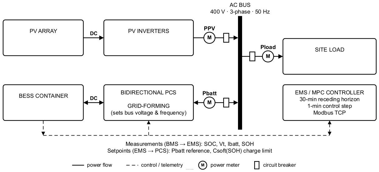
Figure 2.
Second-order Thévenin ECM.
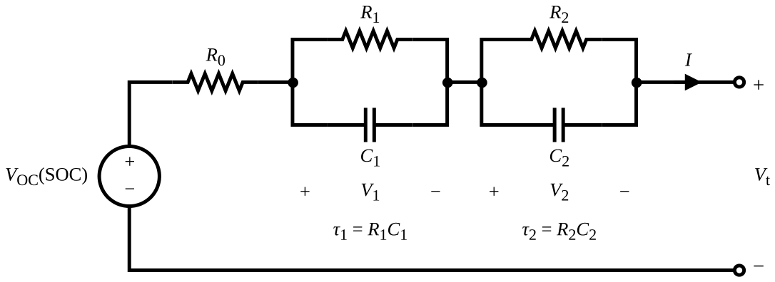
Figure 3.
Conventional rule-based and proposed MPC SOH-aware energy management frameworks.
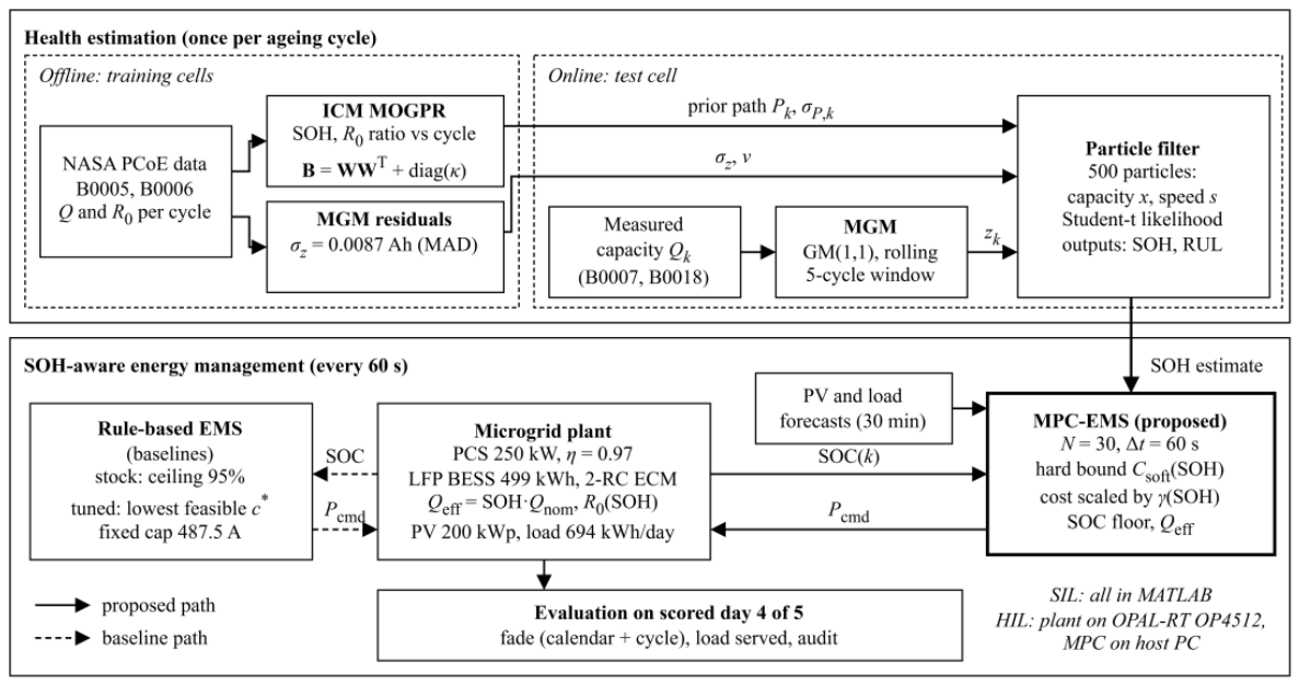
Figure 4.
Particle filter results for the test cells: (a) SOH of B0007; (b) SOH of B0018; (c) RUL of B0007; (d) RUL of B0018.
Figure 4.
Particle filter results for the test cells: (a) SOH of B0007; (b) SOH of B0018; (c) RUL of B0007; (d) RUL of B0018.
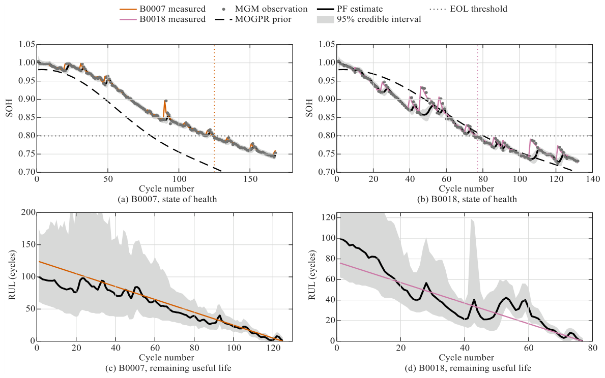
Figure 5.
Scored day at SOH 0.82: (a) PV, load and battery power, (b) SOC with the SOC floor, (c) C-rate against Csoft(SOH) and the rule-based cap.
Figure 5.
Scored day at SOH 0.82: (a) PV, load and battery power, (b) SOC with the SOC floor, (c) C-rate against Csoft(SOH) and the rule-based cap.
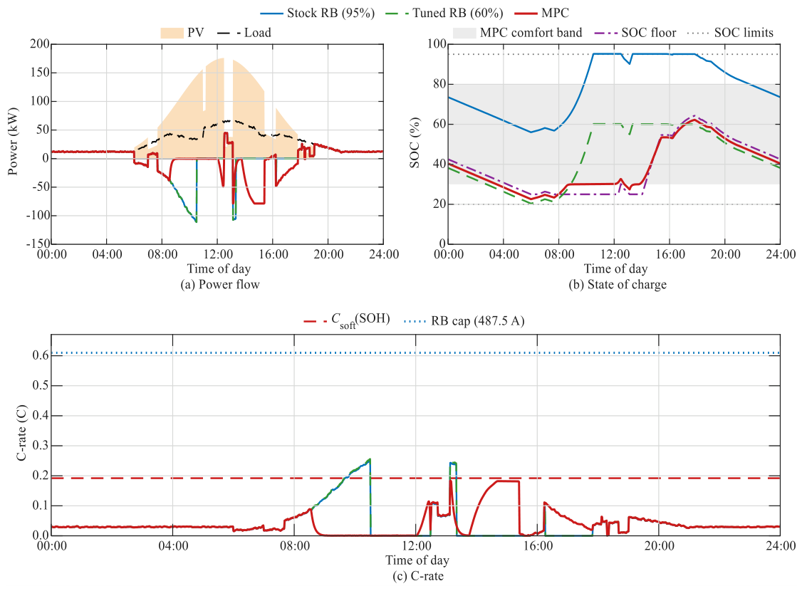
Figure 6.
Daily capacity fade of each controller at SOH 1.00 and 0.82, split into calendar and cycle parts.
Figure 6.
Daily capacity fade of each controller at SOH 1.00 and 0.82, split into calendar and cycle parts.
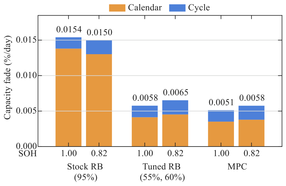
Figure 7.
HIL test set-up.
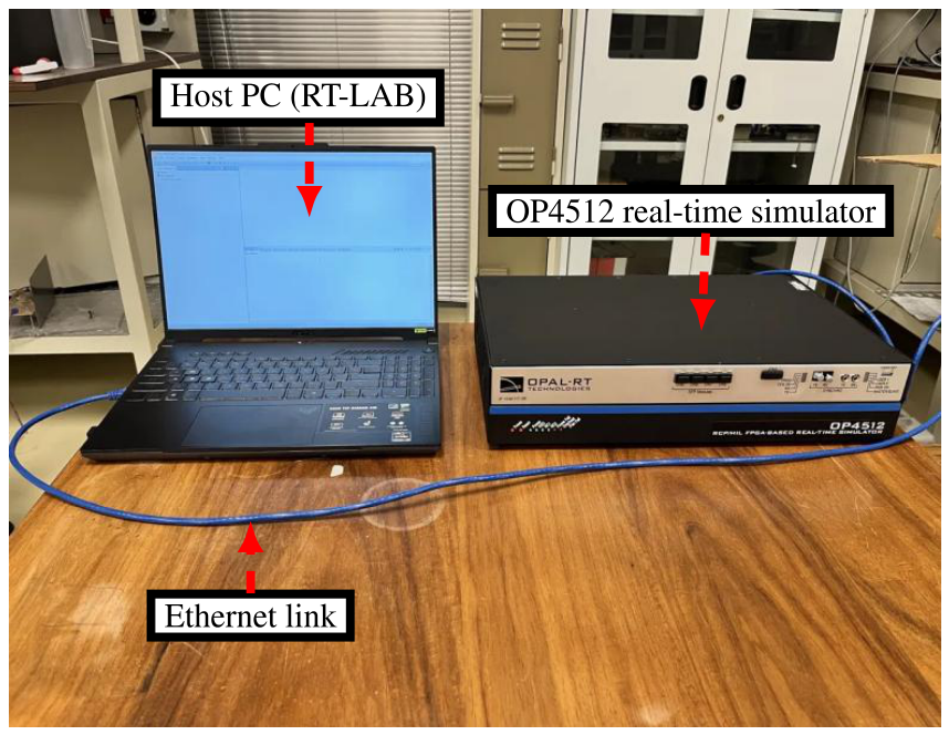
Figure 8.
HIL run over one model day with SOH stepped from 1.00 to 0.82 at 12:00: (a) PV, load and battery power, (b) SOC with the SOC floor, (c) C-rate against Csoft(SOH), (d) MPC solve time against the 1 s control period.
Figure 8.
HIL run over one model day with SOH stepped from 1.00 to 0.82 at 12:00: (a) PV, load and battery power, (b) SOC with the SOC floor, (c) C-rate against Csoft(SOH), (d) MPC solve time against the 1 s control period.
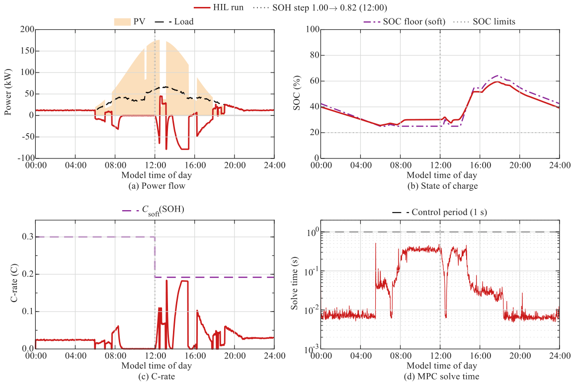

Table 1.
ECM circuit parameters.
| Parameter | Value |
|---|---|
| 76.3 m | |
| 10.2 m | |
| 65.2 m | |
| 880 F | |
| 960 F | |
| 8.98 s | |
| 62.59 s |
Table 2.
Health-estimator settings.
| Symbol | Description | Value |
|---|---|---|
| W | MGM window | 5 cycles |
| σz | Observation scale (train) | 0.0087 Ah |
| Npf | Number of particles | 500 |
| δ | Liu–West discount factor | 0.98 |
| s | Speed-factor bounds | [0.2, 3.0] |
| Neff | Resampling threshold | Npf/2 = 250 |
| H | RUL horizon | 300 cycles |
Table 3.
EMS and evaluation settings.
| Symbol | Description | Value |
|---|---|---|
| N, Δt | Horizon, control step | 30 steps, 60 s |
| Csoft,0 | C-rate limit at SOH 1.00 | 0.30C |
| kSOH | Scheduling slope | 2 |
| ωdeg, ωthr | SOC and throughput weights | 200, 20 |
| ωcyc, ωfloor | Cycling and floor weights | 30, 1500 |
| SOCmin, SOCmax | Hard SOC window | 0.20, 0.95 |
| – | SOC comfort band | 0.30–0.80 |
| Icap | Rule-based current cap | 487.5 A |
| Candidate ceilings | 0.40–0.95 (10 values) | |
| kcal, kSOC | Calendar fade | 0.005%/day, 3.0 |
| kcyc, kC | Cycle fade | 0.004%/EFC, 0.5 |
Table 4.
Case-study microgrid parameters.
| Quantity | Value |
|---|---|
| Load | 694 kWh/day (253.4 MWh/yr), peak 67.4 kW |
| PV array | 200 kWp; 176 kW peak output |
| PV energy | 1152 kWh/day (with cloud cover events) |
| PV inverters | 2 × 100 kW, grid-following |
| PCS | 250 kW, η = 0.97, grid-forming |
| AC bus | 400 V, 3-phase, 50 Hz |
| Battery | LFP, 160S3P × 325 Ah; 512 V, 975 Ah, 499.2 kWh |
| SOC window | 20–95% (374.4 kWh usable when new) |
| Longest deficit | 161 kWh (overnight) |
| Simulation step | 60 s |
Table 5.
Health estimation on the test cells.
| Metric | B0007 | B0018 |
|---|---|---|
| True EOL (cycle) | 125 | 77 |
| MGM one-step RMSE (% of Qnom) | 0.82 | 2.09 |
| MOGPR RMSE (% of Qnom) | 7.09 | 2.42 |
| MOGPR coverage (%) | 86.9 | 100 |
| PF SOH RMSE (pp) | 0.66 | 1.74 |
| PF SOH MAE (pp) | 0.34 | 0.91 |
| PF SOH coverage (%) | 91.7 | 78.8 |
| RUL MAE (cycles) | 9.3 | 9.6 |
| RUL coverage (%) | 100 | 82.9 |
Table 6.
Scored-day results of the three controllers.
| Metric | Stock (SOH 1.00) | Tuned (SOH 1.00) | MPC (SOH 1.00) | Stock (SOH 0.82) | Tuned (SOH 0.82) | MPC (SOH 0.82) |
|---|---|---|---|---|---|---|
| SOC ceiling (%) | 95 | 55 | – | 95 | 60 | – |
| Mean SOC (%) | 81.9 | 41.6 | 36.7 | 79.0 | 43.7 | 38.9 |
| Csoft(SOH) (C) | 0.300 | 0.300 | 0.300 | 0.192 | 0.192 | 0.192 |
| Peak C-rate (C) | 0.205 | 0.205 | 0.188 | 0.250 | 0.250 | 0.183 |
| Steps above Csoft (%) | 0.00 | 0.00 | 0.00 | 4.44 | 4.44 | 0.00 |
| Load served (%) | 100 | 100 | 100 | 100 | 100 | 100 |
| Calendar fade (%/day) | 0.0138 | 0.0041 | 0.0034 | 0.0130 | 0.0045 | 0.0038 |
| Cycle fade (%/day) | 0.0016 | 0.0017 | 0.0017 | 0.0020 | 0.0020 | 0.0020 |
| Total fade (%/day) | 0.0154 | 0.0058 | 0.0051 | 0.0150 | 0.0065 | 0.0058 |
| Degradation reduction vs. stock (%) | – | 62.6 | 66.7 | – | 56.5 | 61.6 |
| Degradation reduction vs. tuned (%) | – | – | 11.1 | – | – | 11.8 |
Disclaimer/Publisher’s Note: The statements, opinions and data contained in all publications are solely those of the individual author(s) and contributor(s) and not of MDPI and/or the editor(s). MDPI and/or the editor(s) disclaim responsibility for any injury to people or property resulting from any ideas, methods, instructions or products referred to in the content. |
© 2026 by the authors. Licensee MDPI, Basel, Switzerland. This article is an open access article distributed under the terms and conditions of the Creative Commons Attribution (CC BY) license (http://creativecommons.org/licenses/by/4.0/).
Copyright: This open access article is published under a Creative Commons CC BY 4.0 license, which permit the free download, distribution, and reuse, provided that the author and preprint are cited in any reuse.