

Submitted:
11 November 2026
Posted:
12 November 2026
You are already at the latest version
Abstract
The allocation of carbon dioxide (CO2) emissions is a critical issue in emissions trading schemes and greenhouse gas (GHG) assessment methodologies. Various modified methods based on energy and exergy approaches have been proposed to allocate CO2 emissions in combined heat and power (CHP) plants; however, a universally accepted approach has not yet been established. While the exergy-based approach has been regarded as the fairest method for CO2 allocation to date, it has not yet been analytically proven. In this study, the Modified Productive Structure Analysis (MOPSA) method, an exergoeconomic analysis, was employed to calculate the incremental cost flow rates for electricity and steam resulting from the imposition of a cost on CO2 emissions from the plant combustor. For CHP plants operating at two heat-to-power ratios (HPRs), CO2 emissions were allocated between heat and electricity in proportion to the increase in their respective cost flow rates. The results indicate that the cost-based method utilizing MOPSA and the CO2 emission allocation method based on exergoeconomic analysis yield allocations similar to those of the exergy-based method for the low-HPR case. However, for the high-HPR case, both methods allocate a slightly larger share of CO2 emissions to electricity than does the exergy-based method.
Keywords:
cogeneration
; CO2 emission allocation
; cost flow rate
; exergy
; exergoeconomics
; heat
; electricity
1. Introduction
Methods of allocating carbon dioxide emissions from power plants to products can contribute to environmental impact assessments and policy development. In particular, combined heat and power (CHP) generation, which produces heat and electricity simultaneously, presents a problem regarding how to distribute greenhouse gas emissions between heat and electricity [1,2]. Since the choice of allocation method significantly impacts energy pricing and emissions trading, emission allocation methods are a matter of scientific and policy interest [3], and various approaches are currently being studied [4,5,6].
The method for allocating carbon dioxide (CO2) emissions for electricity and steam products of CHP power plants was described in earlier studies by Rosen [1,2] and Abusoglu and Kanoglu [3]. The energy-based allocation method assigns carbon dioxide emissions based on the ratio of heat and electricity production rates [1,2,3]. The energy method is simple but fails to reflect qualitative differences between electricity and heat. On the other hand, the exergy-based method allocates emissions based on product exergy content. The exergy method considers heat quality, thereby accounting for qualitative differences between heat and electricity in emission allocation [2]. Allocation may be performed using market prices or supply costs as weights [1,2,3]. Aldrich et al. [4] proposed a method for allocating greenhouse gas (GHG) emissions for CHP systems that accounts for the inefficiencies of the system's components relative to a system with the best efficiency. Gao et al. [5] studied the CO2 distribution problem for biomass gasification CHP systems and coal-fired CHP power plants using exergy and exergoeconomic analyses, respectively. The emission allocation was obtained based on the calculated cost flow rate of the product [5]. Holmberg et al. [6] studied the fuel costs and CO2 emission allocations for heat and electricity in CHP plants that supply heat to pulp and paper mills and electricity to the market. In their study, fuel costs and CO2 emissions were allocated using energy and exergy methods and market-based methods. According to their calculations, the energy method allocated the most CO2 emissions to heat, whereas the exergy and market-based methods allocated more to electricity, and the allocations for heat and electricity were similar for both methods.
Several researchers have conducted comparative studies on allocation methods. Noussan [7] analyzed the annual average operating data of combined heat and power (CHP) plants with heat-to-power ratios (HPR) ranging from 0.57 to 1.55 and calculated the differences in distribution resulting from various allocation methods. He analyzed the nominal performance, annual, and hourly operational data of natural gas-based CHP systems and evaluated the variability of allocation factors based on various technologies, scales, and operating conditions. This analysis confirmed that the exergy method provides allocation factors shifted towards electricity production. He also found that the heat-to-power ratio (HPR) affects the power bonus method (PBM) and heat bonus method (HBM), while the reference efficiency value influences the alternative generation method (AGM). Various allocation methods were applied to combined cycle power plants by Tereshchenko and Nord [8]. In their study, the exergy method was evaluated as the fairest because it reflects the qualitative differences between heat and electricity. However, they discovered that the PBM used as a standard in Europe shows the highest variance in the allocation factors for both electricity and heat. Buchenau et al. [9] evaluated 12 representative emission allocation methods for CHP based on nine evaluation criteria, including applicability, environmental relevance, and systematic accessibility. Among their methods, physical property-based approaches included energy, efficiency, exergy, Dresden, and exergy loss methods, while production-based approaches included replacement, residual value, replacement cost, the Finland method, greenhouse gas (GHG) emissions, and economic value methods. The evaluation results showed that the Finnish method demonstrated the best performance in the standard use case with CO2 emissions of 202 gCO2/kWh_sum; the calculated emission factors for heat and electricity were 192 gCO2/kWh_ht and 322 gCO2/kWh_el, respectively. Additional insights were gained by expressing the allocation factor in terms of CO2 emissions per unit of energy production, as used by this author.
Choi et al. [10] conducted a comparison of emission allowance allocation methods and an assessment of suitability for CHP projects in Korean industrial complexes. Since emission allowance calculation results vary depending on the method and have monetary value, selecting an appropriate allocation method is crucial, and fairness and efficiency must be considered. In their study, they evaluated the change in emission allowances and system performance according to supply temperature and found that the exergy efficiency method (EEM), which has no sensitivity problem and reflects the quality of heat, was the fairest. They also analyzed the differences in emission allowances based on changes in the utilization factor and HPR. There are significant differences in emission allowances based on HPR and the utilization factor across chemical, paper, and other industries. The PBM method has high sensitivity and limitations in reliability, while one of the exergy-based methods, EEM, appears to be most suitable in terms of reflecting thermal quality and fairness in the CHP plants.
In PBM, AGM, and EEM, which were proposed to improve the energy-based allocation method, CO2 allocation values depend on default factors or efficiency. For example, Annex B of EN 15316-4-5: specifies a factor of 1.5 for heat produced by natural gas boilers and 2.5 for electricity produced via CHP, whereas the primary energy factors under current Italian regulations are 1.05 for fuel and 2.42 for electricity [7]. Meanwhile, in AGM, the default efficiency of electricity was set to 41% and the default efficiency of heat was set to 90% for natural gas boilers [7]. In this study, a factor of 1.5 was applied to heat production and 2.5 to electricity production. In addition, the reference efficiencies for heat and electricity were set at 0.90 and 0.40, respectively. The thermal exergy efficiency was set to 0.35. In the light of all the research results, it can be seen that the exergy method provides reasonable and consistent results in various situations. However, there are no analytical or theoretical studies yet that have demonstrated the exergy method to be the optimal approach for allocating CO2 emissions.
In this study, the rates of increase in electricity and steam cost flows were calculated using the Modified Productive Structure Analysis (MOPSA) [11] method for cogeneration plants with two heat-to-power ratios (HPRs), assuming that CO2 emission costs are imposed on the emissions generated in the combustor. Carbon dioxide emissions were allocated to electricity and heat products based on the increase in the cost flow rates of electricity and steam. According to the calculation results, the CO2 emission allocation through the MOPSA method was close to that obtained through the exergy method. In addition, the exergy method was compared with other allocation methods, and the results were discussed.
2. Cogeneration Plants for Heat and Electricity Production
Figure 1 shows a schematic diagram of a 430 MW combined cycle cogeneration plant modified from a 500 MW combined cycle power plant [11]. All state points considered in this analysis are shown in this figure. The schematic shows ten components: <1> air compressor (AC), <2> combustor (COM), <3> gas turbine (GT), <4> fuel preheater (FPH), <5> steam turbines (ST), <6> condenser (CON), <7> condensate pump (CP), <8, 9> two feed pumps (FP-A, FP-B), <10> heat recovery steam generator (HRSG). As can be seen in Figure 1, the high-pressure (HP) superheater supplies steam (522) to the HP steam turbine, and the intermediate-pressure (IP) superheater supplies steam (524) to the IP steam turbine. Meanwhile, steam is extracted from the low-pressure (LP) superheater and the HP steam turbine. The steam from the IP steam turbine flows into the LP steam turbine. The steam exiting the LP steam turbine flows to the condenser. The extracted steam flow rates at state points (518), and (502) were adjusted to satisfy the second law of thermodynamics for the HRSG and HPT. Figure 2 shows a 300 MW-class gas turbine combined heat and power (CHP) plant constructed to utilize the steam flow supplied to the steam turbine shown in Figure 1 as process steam, thereby increasing the HPR. The water required for the HRSG is supplied by a pump <5> in this plant. The flow rate of the extraction steam from the HRSG has been adjusted to match the proper operation of the HRSG. The HPRs of the two cogeneration systems are significantly different. The HPR of the power plant in Figure 1 is 0.59, and the HPR of the power plant in Figure 2 is 1.88. However, conducting research by generating scenarios across a diverse range of HPR values presents a non-trivial challenge.
The molar flow rates of fuel, air, and steam (or water) and thermodynamic state quantities such as temperature and pressure for the 430 MW combined cycle cogeneration plant and for part of the 300 MW gas turbine cogeneration plant are shown in Table 1a. Table 1b presents thermodynamic property data for a gas turbine cogeneration system, showing different thermodynamic state quantities at the same state points as in Figure 1. The thermodynamic properties such as molar flow rate, pressure and temperature at various state points shown in Table 1a were the design/ initial operation data for the 500 MW combined cycle plant [11]. Mass flow rate data at state points 518, 522, and 524 in Table 1b were adjusted to ensure the smooth operation of the HRSG within the gas turbine cogeneration plant. Other thermodynamic properties, including enthalpy and entropy, were calculated using polynomial correlations [12] fitted to the thermophysical data in the JANAF Tables [13]. The thermophysical properties of water and steam were evaluated using the equations recommended by the International Formulation Committee (IFC) [14]. Calculated values of enthalpy, entropy and exergy flow rates are also given in this table. Each state point is identified by a three-digit number, where the first number is 1 for air flow, 3 for fuel flow, 5 for water or steam flow, and 6 for flue gas flow.

Table 1a.
Property values, calculated enthalpy and entropy flow rates, thermal and mechanical exergy flows at various state points in the combined cycle cogeneration plant at 100% load condition.
Table 1a.
Property values, calculated enthalpy and entropy flow rates, thermal and mechanical exergy flows at various state points in the combined cycle cogeneration plant at 100% load condition.
| States | n [kmol/s] | T [K] |
P [kPa] |
[kJ/s] |
[kJ/sK] |
[kJ/s] |
[kJ/s] |
|---|---|---|---|---|---|---|---|
| 101 | 29.780 | 288.2 | 102.5 | 12,991.3 | 204.5 | 50.2 | 851.2 |
| 102 | 29.780 | 596.7 | 1025.0 | 287,459.2 | 279.9 | 82,075.6 | 170,833.5 |
| 301 | 0.966 | 288.2 | 102.5 | 543.6 | 3.6 | 6.3 | 27.6 |
| 302/303 | 0.966 | 453.2 | 102.5 | 7481.4 | 22.5 | 1322.1 | 27.6 |
| 304 | 0.966 | 688.5 | 1025.0 | 20,293.6 | 26.5 | 7405.9 | 5540.9 |
| 501/522 | 3.886 | 835.2 | 12,840.0 | 245,129.2 | 465.6 | 105,736.3 | 891.7 |
| 502 | 3.886 | 606.0 | 2660.0 | 215,936.9 | 472.2 | 75,277.4 | 179.5 |
| 503/524 | 4.718 | 829.1 | 2360.0 | 304,927.3 | 638.1 | 114,873.9 | 192.4 |
| 504/505 | 4.718 | 490.3 | 160.0 | 247,072.1 | 653.2 | 52,708.2 | 5.0 |
| 506/531 | 4.718 | 320.0 | 10.0 | 219,869.9 | 693.4 | 13,541.5 | -7.8 |
| 511 | 10.402 | 322.1 | 1580.0 | 38,604.0 | 129.0 | 711.7 | 277.8 |
| 512 | 8.373 | 424.6 | 629.0 | 96,273.7 | 279.9 | 13,428.6 | 79.8 |
| 513 | 5.455 | 427.7 | 16,960.0 | 65,030.9 | 183.7 | 9059.8 | 1655.4 |
| 515 | 1.783 | 452.3 | 3650.0 | 24,420.7 | 68.3 | 4089.7 | 114.2 |
| 516/571 | 0.617 | 493.3 | 3540.0 | 10,494.0 | 28.0 | 2170.0 | 38.3 |
| 518 | 0.833 | 541.0 | 483.0 | 44,979.3 | 110.4 | 12,133.5 | 5.7 |
| 525 | 0.786 | 452.3 | 3650.0 | 10,774.1 | 30.1 | 1804.3 | 50.4 |
| 532 | 5.684 | 306.4 | 15.0 | 14,236.7 | 49.2 | 47.4 | -8.9 |
| 533 | 0.349 | 307.5 | 2040.0 | 913.2 | 3.1 | 3.7 | 12.2 |
| 535/572 | 0.617 | 346.1 | 3540.0 | 3423.7 | 11.0 | 161.7 | 38.3 |
| 539 | 4.718 | 301.0 | 2140.0 | 10,084.1 | 34.5 | 4.8 | 173.7 |
| 549 | 333.056 | 293.2 | 230.0 | 504,455.4 | 1777.5 | 1063.5 | 774.2 |
| 550 | 333.056 | 300.0 | 160.0 | 675,859.4 | 2356.9 | 143.3 | 353.0 |
| 561 | 5.684 | 300.0 | 16.0 | 11,519.9 | 40.2 | 2.4 | -8.8 |
| 562 | 10.402 | 301.0 | 2140.0 | 22,231.2 | 76.1 | 10.6 | 382.9 |
| 563 | 2.917 | 424.6 | 671.0 | 33,546.8 | 97.5 | 4678.9 | 30.0 |
| 564 | 2.917 | 425.0 | 3650.0 | 33,736.0 | 97.6 | 4698.4 | 186.9 |
| 565 | 5.455 | 424.6 | 671.0 | 62,731.5 | 182.4 | 8749.4 | 56.1 |
| 566 | 5.455 | 426.9 | 16,960.0 | 64,665.8 | 182.8 | 8949.5 | 1655.4 |
| 602/603 | 30.746 | 1403.9 | 1025.0 | 1,361,848.3 | 1329.2 | 799,513.7 | 176,374.4 |
| 604/605 | 30.746 | 865.9 | 107.1 | 658,404.0 | 1278.5 | 283,351.3 | 4224.7 |
| 606 | 30.746 | 351.2 | 103.0 | 80,744.8 | 286.6 | 4386.7 | 1249.6 |
Table 1b.
Property values, calculated enthalpy and entropy flow rates, thermal and mechanical exergy flows at various state points in the gas turbine cogeneration plant at 100% load condition.
Table 1b.
Property values, calculated enthalpy and entropy flow rates, thermal and mechanical exergy flows at various state points in the gas turbine cogeneration plant at 100% load condition.
| States | n [kmol/s] | T [K] |
P [kPa] |
[kJ/s] |
[kJ/sK] |
[kJ/s] |
[kJ/s] |
|---|---|---|---|---|---|---|---|
| 518 | 1.110 | 541.0 | 480.0 | 59,972.5 | 147.2 | 16,178.0 | 7.7 |
| 522 | 3.886 | 835.2 | 12,840.0 | 245,129.2 | 465.6 | 105,736.3 | 891.7 |
| 524 | 4.441 | 830.5 | 2420.0 | 287,195.7 | 599.9 | 108,515.7 | 185.9 |
| 525 | 0.777 | 452.3 | 3650.0 | 10,647.1 | 29.8 | 1783.1 | 49.8 |
| 561 | 9.437 | 298.2 | 103.0 | 17,826.1 | 62.4 | 0.0 | 0.2856 |
| 562 | 9.437 | 298.6 | 2140.0 | 18,430.0 | 63.2 | 0.2 | 347.4 |
| 563 | 2.917 | 424.6 | 671.0 | 33,546.8 | 97.5 | 4678.9 | 30.0 |
| 564 | 2.917 | 425.0 | 3650.0 | 33,736.0 | 97.6 | 4698.4 | 186.9 |
| 565 | 5.455 | 424.6 | 671.0 | 62,731.5 | 182.4 | 8749.4 | 56.1 |
| 566 | 5.455 | 426.8 | 16,960.0 | 64,665.8 | 182.8 | 8949.5 | 1655.4 |
| 606 | 30.746 | 356.3 | 103.0 | 86,075.0 | 301.7 | 5223.8 | 1249.6 |
3. Various Methods of CO2 Allocation
This section reviews and examines various methods for CO2 emission allocation in CHP plants. CHP plants allocate primary energy production into heat and electricity. One method of CO2 allocation is based on the energy or exergy output of CHP plants. The allocation factors for heat and electricity by the energy method are as follows.
whereEQ and EW are the heat energy and electricity production, respectively and fQ_ENG and fW_ENG denote the fractions of CO2 emissions allocated to heat and electricity production, respectively. Here ηQ(=EQ/Ein) and ηW(=EW/Ein) represent the energy efficiency of heat and electricity, respectively, to the energy input of the power plant,Ein. The sum of heat and electricity produced is less than the energy input, and the overall efficiency, ηT(=ηQ + ηW) is less than 1 [10].
The allocation factors based on exergy are as follows.
Here ExQ and ExW are heat exergy and electricity production and ηx,Q(=ExQ/Exin) and ηx,W(=ExW/Exin) represent the exergy efficiency of heat and work, respectively, relative to the power plant’s exergy input, Exin (typically identical to the energy input). Because the exergy efficiency of heat is lower than the energy efficiency of heat, the allocation factor for heat in the energy method is greater than that in the exergy method.
The Dresden method, which was proposed by Zschernig and Sander [15], is a modified version of exergy method. In this method, the electricity loss caused by the heat extraction is calculated using the value obtained using the following relationship.
Here Tcond and TQ represent the condensing temperature and outlet temperature of extracted steam, respectively, and vP represents the process quality, which is taken as 0.8 in this study. Equation (5) approximates heat extraction as work using Carnot efficiency. Using the power values obtained in this way, the heat and electricity allocation factors according to the Dresden method are as follows.
Another approach is to allocate CO2 emission between heat and power production in proportion to the fuel required to generate the same amount of heat and electricity in separate power plants operating at default efficiencies. One such method is AGM, and the allocation factors for heat and power are as follows:
Here ηQ,refand ηW,ref represent the default energy efficiency of heat and work, respectively, and are generally set to 0.90 and 0.40 [7], respectively. The Finnish method [9] is the same as the AGM. However, in the study by Buchenau et al. [9], the default efficiencies for heat and power in the Finnish method were set at 0.89 and 0.53, respectively. If we replace the energy for heat in Equations (8) and (9) with the exergy for heat, we obtain the following exergy efficiency method (EEM) [9]. AGM allocates emissions using energy outputs and reference energy efficiencies, whereas EEM uses exergy outputs and reference exergy efficiencies. The EEM method presented in Equations (10) and (11) provides values similar to the exergy method because the default exergy efficiencies of heat and electricity have similar values.
The power bonus method, designed to utilize district heating systems, can also be applied to combined heat and power plants. The primary energy factor for any CHP plant analogous to a district heating system may be written as follows [7].
With the help of Equation (12), the allocation factor for heat and electricity can be written as
Here fF,f, and fW,f represent the default weighting factor of fuel and electricity, which are taken as 1.05 and 2.5, respectively, in this study [7]. On the other hand, the heat bonus method (HBM) has the following allocation factor for electricity and heat [7].
Finally, the allocation of carbon dioxide emissions can be based on the economic value of the product. For example, it can be allocated using the unit costs of heat and electricity paid by consumers. In this case, the allocation factors for heat and electricity are given as follows [1,7].
Here cQ and cW represent the unit cost of heat and electricity, respectively; in this study, the current prices in Korea—$30/GJ and $70/GJ—were used. The unit cost of heat and electricity obtained through exergoeconomic analysis [5] could also be used. In this approach, the energy values for heat and work in Equations (17) and (18) must be replaced with exergy values.
4. Mass and Energy Conservation and Exergy-Balance Equations
This section presents the mass and energy conservation principles and exergy analysis for each component of the combined cycle cogeneration and gas turbine cogeneration plants. The mass and energy flows entering and exiting each device must satisfy the following conservation equations.
- Mass conservation equation
Based on the first and second laws of thermodynamics, the following exergy-balance equation for material flows into and out of each component was derived [16]:
In Equation (21), the superscripts CHE and W represent chemical and work exergy, respectively, while T and P represent thermal and mechanical exergy, respectively. The fourth term on the left side represents the negative value of the lost work rate due to entropy generation, defined by the Gouy-Stodola theorem as follows [17].
The irreversibility rate can be obtained with the help of the heat transfer rate obtained from the conservation of energy given in Equation (20).
The exergy flow is expressed as follows:
Exergy per unit mass (ex) can be expressed based on reference temperature (Tref) and reference pressure (Pref):
The reference temperature and pressure used in Equation (24) generally correspond to ambient conditions, with values of Tref = 298.15 K and Pref = 101.3 kPa. For the exergoeconomic analysis of a combined cycle cogeneration plant, an exergy-balance equation for each component based on Equation (21) is essential, as shown in Table 2. The exergy per unit mass (ex) can be decomposed into thermal exergy, which is associated with temperature, and mechanical exergy, which is associated with pressure [18]. Detailed procedures for evaluating the thermal and mechanical exergy components are provided by Uysal et al. [19]. As shown in Table 2, the exergy was decomposed into thermal and mechanical parts.
5. Modified Productive Structure Analysis: Exergoeconomic Analysis
Modified Productive Structure Analysis (MOPSA) [17,20], is an exergoeconomic method that formulates the exergy cost-balance equation by assigning different unit costs to the various types of exergy flows in the exergy-balance equation of Equation (21). For instance, the following general exergy cost-balance equation of Equation (25) is obtained with the consideration of unit costs of every process such as co the unit cost of fuel, cT the unit cost of thermal exergy, cP the unit cost of mechanical exergy, cS the unit cost of lost work, and cW the unit cost of work or electricity in the exergy-balance equation.
The exergy cost-balance equation is commonly established by analyzing the differences between the exergy quantities entering and exiting each device. This approach is particularly useful for calculating the cost flows associated with exergy when the exergy of a material changes as it passes through a device. In the cost-balance equation for each component, a new unit cost, expressed in Gothic font, is assigned to the product that represents the characteristics of the component as follows, which is called “principal product’”. For example, in the case of an air compressor, a new unit cost is assigned to the mechanical exergy of air because the compressor's primary goal is to increase air pressure. The cost balance equation for all components of a combined cycle cogeneration plant can be obtained by applying Equation (25) to 10 components as shown in Table 3. As can be seen from the 10 cost-balance equations for the 10 components, 17 unknown unit costs appear, so seven additional equations are needed to solve the cost-balance equations. Six additional equations can be obtained by considering the junctions for various exergy flows, such as thermal and mechanical exergy flows of air, fuel and flue gas, thermal and mechanical exergy flows of water or steam, work done in gas turbines, and work done in steam turbines. Finally, we can obtain one equation from the "boundary" component of the power plant. The "boundary" component has special characteristics of discharging waste from the power plant into the environment. All waste exiting through the boundary affects the environment. By solving the 10 cost-balance equations for the components and seven auxiliary equations simultaneously, 17 unknown unit costs can be obtained.
In the cost-balance equation in Equation (25), represents the cost flow per unit time, which includes both the initial purchase cost and the operating cost of the k-th component. It is calculated using the following equation [21]:
In Equation (26), ϕkand δk are the maintenance cost factor and annual operation time, respectively. In Equation (26) is the initial investment of the component converted into an annual equivalent cost, which is given as follows.
In Equation (27), SV is salvage value after n years of the device's life and PWF and CRF denote the present value factor and the capital recovery factor, respectively.
6. Calculation Results and Discussion
Table 4 shows the calculated exergy flow rates for each component of the combined cycle cogeneration plant. The fifth column of this table represents exergy destruction due to changes in the inflow and outflow of entropy flow in each device, and the sixth column represents exergy destruction due to heat transfer interactions between each component and the environment. The heat transfer can be obtained from the first law of thermodynamics for each component, Equation (20). The negative sign of the heat transfer indicates an inflow of heat to the corresponding component and consequently increases the exergy destruction of the component as can be seen from the Gouy-Stodola theorem in Equation (22).
The total exergy destruction rate for the combined cycle cogeneration plant is approximately 854.1 MW (Sum of fifth and sixth column in Table 4). The amounts of electricity produced by the gas turbine and steam turbine are approximately 603.7 MW and 140.1 MW, respectively, and the air compressor consumes 286.0 MW of the electricity produced by the gas turbine. The maximum output of the combined-cycle cogeneration plant, accounting for a generator efficiency of 95%, is approximately 435.0 MW. Since the enthalpy flow rate and exergy flow rate of the extracted steam at state points 502 and 518 are 260.9 MW and 87.4 MW (Table 1a), respectively, the HPR of this combined cycle cogeneration plant is approximately 0.59 (=260.9 MW/443.6 MW). In this study, the exergy of steam extracted from the combined-cycle cogeneration plant was considered as the output exergy at state points 502 and 518. In this table, the exergy rate of the product is represented by a positive value, while the exergy rate of the resource is represented by a negative value. The sum of all exergy flows, including irreversibilities, is equal to the heat input of 1373.3 MW into the combustor—that is, the heat of reaction within the combustor. The energy and exergy efficiencies of the cogeneration plant may be obtained by the following equation.
According to Equations (28) and (29), the energy efficiency and exergy efficiency of the combined cycle cogeneration plant are approximately 51.3%, and 38.7%, respectively.
The initial investment costs for the air compressor, combustor, gas turbine, fuel preheater, steam turbine, condenser, condensate pump, two feedwater pumps, and heat recovery steam generator are $38.7 million, $5.0 million, $35.0 million, $3.0 million, $45.9 million, $8.5 million, $0.55 million, $0.65 million, $0.74 million and $17.7 million, respectively. This initial investment data was obtained from a 500 MW combined-cycle power plant constructed in Korea in 2024. The total initial investment for the combined cycle power plant was approximately $155.7 million. While existing data was used for the operating data at specific state points of the combined-cycle cogeneration plant [11], the initial investment costs were updated with the latest data. Applying an annual operating time of 8000 hours, an equipment lifespan of 20 years, an annual interest rate of 10%, and a depreciation rate of 12% after 20 years, the input cost flow per second for the combined cycle cogeneration plant, including maintenance, operating costs, and fuel costs, is approximately $18.0/s (6th column in Table 5b). The unit fuel cost of natural gas was set at $20.0/GJ in this calculation. The natural gas supplied to the combustor consists of 90.0% methane, 6.1% ethane, 2.6% propane, and 1.3% butane. The mass and lower heating value (LHV) of the fuel supplied to the fuel preheater are approximately 18.12 kg/kmol and 48,918.1 kJ/kg, respectively; these data were used to calculate the cost flow rate of the fuel.
Table 5a shows the unit cost of principal products by component of a 430 MW combined cycle cogeneration plant and the unit cost of thermal and mechanical exergy flows of gas (cT, andcP) and water (cDT, andcDP). The unit costs shown in Table 5a were obtained by solving the 17 cost- balance equations described in Table 3. The unit cost of electricity (c3W), the main product of gas turbines, is approximately $40.65/GJ (=$0.146/kWh). On the other hand, the unit cost of electricity produced by steam turbines (c5DW) is approximately $44.93/GJ (=$0.162/kWh), which is higher than that of electricity produced by gas turbines. The reason the unit cost of electricity produced by steam turbines is higher is that the efficiency of steam turbines is lower than that of gas turbines. As can be seen in Table 5a, the main product of the HRSG (c10DT) is steam, and the unit cost of steam is approximately $36.41/GJ. However, to calculate the cost flow rate of extracted steam at state points 502 and 518, it is better to use the thermal exergy unit cost of steam (cDT, and cDP). The unit cost of the loss cost flow (cS) is approximately -$4.13/GJ. The same sign convention for the cost flow rates related to products and resources was used as the case of exergy-balances shown in Table 4. As can be seen in Table 5b, the loss cost flow rate in each component turns out to be negative, which indicates that the loss cost flow due to exergy destruction increases the operational burden of the plant.
Table 5a.
Unit cost of principal products for each component obtained through the cost balance equation of a combined cycle cogeneration plant. (Unit is $/GJ).
Table 5a.
Unit cost of principal products for each component obtained through the cost balance equation of a combined cycle cogeneration plant. (Unit is $/GJ).
| c1P | c2T | c3W | c4T | c5DW |
| 56.84 | 3.35 | 40.65 | 13,242.5 | 44.93 |
| c6DT | c7DP | c8DP | c9DP | c10DT |
| -16.42 | 1370.2 | 73.73 | 58.25 | 36.41 |
| cT | cP | cDT | cDP | cW |
| 27.63 | 56.84 | 39.94 | 298.64 | 40.65 |
| cDW | cS | |||
| 44.93 | -4.13 |
Table 5b.
Various exergy cost flow rates, loss cost flow rates, and investment cost flow rates of each component of a combined cycle cogeneration plant. Unit is $/s.
Table 5b.
Various exergy cost flow rates, loss cost flow rates, and investment cost flow rates of each component of a combined cycle cogeneration plant. Unit is $/s.
| Component | Thermal | Mechan | Work(Steam*) | Lost cost | Investment |
|---|---|---|---|---|---|
| AC | 2.2661 | 9.6623 | -11.6241 | -0.1401 | -0.1643 |
| COM | 2.3969 | 0.3134 | 0.0 | -2.6891 | -0.0212 |
| GT | -14.2601 | -9.7855 | 24.5433 | -0.3491 | -0.1486 |
| FPH | 17.3435 | 0.0 | 0.0 | -0.0029 | -17.3407 |
| ST | -5.8052 | -0.2702 | 6.2955 | -0.0252 | -0.1949 |
| CON | 0.0 | -0.1412 | 0.2394* | -0.0621 | -0.0361 |
| CP | 0.0003 | 0.5367 | -0.5347 | 0.0 | -0.0023 |
| FPA | 0.0008 | 0.0116 | -0.0094 | -0.0001 | -0.0028 |
| FPB | 0.0080 | 0.0932 | -0.0966 | -0.0014 | -0.0031 |
| HRSG | -7.7070 | -0.4825 | 8.4723* | -0.2077 | -0.0752 |
| Total | -5.7567 | -0.0622 | 18.5740(8.7117*) | -3.4777 | -17.9892 |
Various exergy-related flows, including thermal, mechanical, steam, and electricity cost flows, as well as loss cost flows and investment cost flows, are shown in Table 5b. These cost flows can be obtained by multiplying the exergy flow rate by the corresponding unit cost. As can be seen in this table, investment costs (-$17.99/s) are almost fully recovered through power production (Fourth column in Table 5b), $18.57/s, whereas the loss cost flow (-$3.48/s) is partially recovered through steam production ($8.71/s). The reason steam cost flow and loss cost flow are related is that steam extracted from the HRSG or turbine is discharged into the environment. The cost flow rate of electricity generated by a combined-cycle cogeneration plant is approximately $18.57/s, which can be utilized as data for CO2 emission allocations.
Table 6a shows the increase in unit cost of principal products for each component of a 430 MW combined cycle cogeneration plant when a cost is imposed on carbon dioxide produced in the combustor. If a price of $0.1 per kg is applied to CO2, the unit cost of electricity produced by gas turbines increases from $40.65/GJ to $51.86/GJ, and the unit cost of electricity produced by steam turbines increases from $44.93/GJ to $57.0/GJ. The unit cost of thermal exergy at state points 502 and 518 increases from $39.94/GJ to $51.05/GJ. As can be seen in Table 5b and 6b, if CO2 is charged at a cost of $0.1/kg, that is, an increase of $4.92/s in the combustor input cost flow rate, it causes an increase of $5.08/s in the electricity cost flow rate and an increase of $0.986/s in the extracted steam cost flow rate. The increase in the cost flow rate of electricity can be calculated by subtracting the sum of the cost flow rates of electricity presented in Table 5b from the sum of the cost flow rates of electricity presented in Table 6b. Changes in extracted steam cost flow rates can be calculated approximately using the following method.
where ΔcDT and ΔcDP represent the changes in the unit costs of thermal and mechanical exergy when CO2 emission costs are applied versus when they are not. Equation (30) provides approximately $0.986/s for the increase in the cost flow rate of extracted steam. What is clear is that the incremental steam cost flow rate for the extracted steam corresponds to approximately half of the incremental steam cost flow rate (about $2.40/s) calculated by subtracting the sum of the steam cost flow rates in Table 5b from the sum of the steam cost flow rates presented in Table 6b. Even if the sum of the cost increase flow rates for heat and electricity exceeds the CO2 input cost flow rate, the ratio of the cost increase flow rates for heat and electricity can be estimated. The increased cost flow rate values of extracted steam and electricity provide the carbon dioxide allocation for heat and power production, which is approximately 0.1625 for heat production and approximately 0.8375 for power production as shown in Table 10a.
Table 6a.
Unit costs of principal products for each component obtained through the cost-balance equation of a combined cycle cogeneration plant when including carbon dioxide emission costs. (Unit is $/GJ).
Table 6a.
Unit costs of principal products for each component obtained through the cost-balance equation of a combined cycle cogeneration plant when including carbon dioxide emission costs. (Unit is $/GJ).
| c1P | c2T | c3W | c4T | c5DW |
| 72.16 | 11.14 | 51.86 | 13,260.1 | 57.00 |
| c6DT | c7DP | c8DP | c9DP | c10DT |
| -20.17 | 1736.9 | 88.79 | 73.34 | 46.58 |
| cT | cP | cDT | cDP | cW |
| 35.44 | 72.16 | 51.05 | 377.85 | 51.86 |
| cDW | cS | |||
| 57.00 | -5.28 |
Table 6b.
Various exergy cost flow rates, loss cost flow rates, and investment cost flow rates of each component of a combined cycle cogeneration plant when including carbon dioxide emission costs. Unit is $/s.
Table 6b.
Various exergy cost flow rates, loss cost flow rates, and investment cost flow rates of each component of a combined cycle cogeneration plant when including carbon dioxide emission costs. Unit is $/s.
| Component | Thermal | Mechan | Work(Steam*) | Lost cost | Investment |
|---|---|---|---|---|---|
| AC | 2.9072 | 12.2652 | -14.8291 | -0.1790 | -0.1643 |
| COM | 7.9806 | 0.3978 | 0.0 | -3.4375 | -4.9410 |
| GT | -18.2940 | -12.4216 | 31.3104 | -0.4462 | -0.1486 |
| FPH | 17.3443 | 0.0 | 0.0 | -0.0037 | -17.3407 |
| ST | -7.4187 | -0.3418 | 7.9876 | -0.0322 | -0.1949 |
| CON | 0.0 | -0.1786 | 0.2941* | -0.0794 | -0.0361 |
| CP | 0.0004 | 0.6803 | -0.6784 | 0.0 | -0.0023 |
| FPA | 0.0010 | 0.0139 | -0.0120 | -0.0002 | -0.0028 |
| FPB | 0.0102 | 0.1173 | -0.1225 | -0.0019 | -0.0031 |
| HRSG | -9.8872 | -0.6112 | 10.8389 | -0.2654 | -0.0752 |
| Total | -7.3562 | -0.0787 | 23.6560(11.1330*) | -4.4455 | -22.9090 |
An analysis similar to that performed on the combined cycle cogeneration plant can also be performed on gas turbine cogeneration plant. Table 7 shows the calculated exergy flow rates for each component of the gas turbine cogeneration plant. The fifth column of this table represents exergy destruction due to changes in the inflow and outflow of entropy flow in each device, and the sixth column represents exergy destruction due to heat transfer interactions between each component and the environment. The total exergy destruction rate for the gas turbine cogeneration plant is approximately 851.2 MW, which is similar to that of combined cycle cogeneration plant. The amount of electricity produced by the gas turbine is approximately 603.7 MW, and the air compressor and pump consume 289.2 MW of the electricity produced by the gas turbine. The maximum output of the gas turbine cogeneration plant, accounting for a generator efficiency of 95%, is approximately 300 MW. Since the enthalpy flow rate and exergy flow rate of the extracted steam at state points 518, 522, and 524 are 592.3 MW and 231.5 MW, respectively, the HPR of this gas turbine cogeneration plant is approximately 1.88 (=592.3 MW/314.5 MW). The sum of all exergy flows, including irreversibility, is equal to the heat input of 1372.2 MW in the combustor. According to Equations (28) and (29), the energy efficiency and exergy efficiency of the gas turbine cogeneration plant are approximately 66.0%, and 40.0%, respectively.
Table 8a shows the unit cost of principal products by component of a 300 MW gas turbine cogeneration plant and the unit cost of thermal and mechanical exergy flows of gas and water. The unit cost of electricity (c3W)—the primary output of the gas turbine—is approximately $54.19/GJ (=$0.195/kWh), which is significantly higher than the cost of electricity produced by a combined cycle cogeneration plant. The unit cost of extracted steam (cDT) is approximately $47.03/GJ, which is slightly lower than the unit cost of electricity. The unit cost associated with exergy destruction is approximately -$11.61/GJ, which is larger in absolute value than that of the combined cycle cogeneration plant. Table 8b presents various exergy-related flows—including thermal, mechanical, electrical, and steam cost flows—as well as cost flows associated with losses and investment. As can be seen in this table, investment cost flow rate (-$17.76/s) is almost entirely recovered through power production ($17.04/s), while loss cost flow rate (-$9.70/s) is partially recovered through steam production ($10.84/s) and the remainder is discharged into the environment through exergy flow. This is because the majority of the extracted steam is equal to the outlet flow rate of the HRSG.
Table 8a.
Unit costs of principal products for each component obtained through the cost-balance equations for the gas turbine cogeneration plant (Unit is $/GJ).
Table 8a.
Unit costs of principal products for each component obtained through the cost-balance equations for the gas turbine cogeneration plant (Unit is $/GJ).
| c1P | c2T | c3W | c4T | c5DP |
| 77.36 | 10.88 | 54.19 | 13,257.3 | 122.31 |
| c6DP | c7DP | c8DT | cT | cP |
| 97.91 | 82.50 | 47.03 | 35.38 | 77.37 |
| cDT | cDP | cW | cS | |
| 47.03 | 90.22 | 54.19 | -11.61 |
Table 8b.
Various exergy cost flow rates, loss cost flow rates, and investment cost flow rates of each component of a gas turbine cogeneration plant. Unit is $/s.
Table 8b.
Various exergy cost flow rates, loss cost flow rates, and investment cost flow rates of each component of a gas turbine cogeneration plant. Unit is $/s.
| Component | Thermal | Mechan | Work(Steam*) | Lost cost | Investment |
|---|---|---|---|---|---|
| AC | 2.9020 | 13.1508 | -15.4944 | -0.3940 | -0.1643 |
| COM | 7.7225 | -7.7012 | -0.0212 | ||
| GT | -18.2601 | -13.3240 | 32.7153 | -0.9825 | -0.1486 |
| FPH | 17.3487 | -0.0080 | -17.3407 | ||
| CP | 0.0425 | -0.0364 | -0.0038 | -0.0023 | |
| FPA | 0.0009 | 0.0154 | -0.0128 | -0.0007 | -0.0028 |
| FPB | 0.0094 | 0.1319 | -0.1310 | -0.0072 | -0.0031 |
| HRSG | -9.8399 | -0.3198 | 10.8352* | -0.6003 | -0.0752 |
| Total | -0.1165 | -0.3032 | 17.0407(10.8352*) | -9.6977 | -17.7582 |
Table 9a shows the increase in unit cost of principal products for each component of a 300 MW gas turbine cogeneration plant when a cost is imposed on CO2 produced in the combustor. If a price of $0.1 per kg is applied to CO2, the unit cost of electricity produced by gas turbines increases from $54.19/GJ to $69.19/GJ (c3W). The unit cost of steam exergy at state points 518, 522 and 524 increases from $47.03/GJ to $60.19/GJ (cDT). As can be seen in Table 8b and 9b, if CO2 is charged at a cost of $0.1/kg, that is, an increase of $4.92/s in the combustor input cost flow rate, it causes an increase of $4.719/s in the electricity cost flow rate and an increase of $3.065/s in the extracted steam cost flow rate. The increase in the cost flow rate of the extracted steam can be obtained by the following equation.
The increased value of extracted steam and electricity provides CO2 allocation for heat and power production, which is approximately 0.3938 for heat production and approximately 0.6062 for power production, as shown in Table 10a.
Table 9a.
Unit costs of principal products for each component obtained through the cost-balance equation of a gas turbine cogeneration plant when including carbon dioxide emission costs. Unit is $/GJ.
Table 9a.
Unit costs of principal products for each component obtained through the cost-balance equation of a gas turbine cogeneration plant when including carbon dioxide emission costs. Unit is $/GJ.
| c1P | c2T | c3W | c4T | c5DP |
| 98.44 | 20.84 | 69.19 | 13,279.1 | 154.35 |
| c6DP | c7DP | c8DT | cT | cP |
| 120.14 | 104.80 | 60.19 | 45.37 | 98.44 |
| cDT | cDP | cW | cS | |
| 60.19 | 114.12 | 69.19 | -14.86 |
Table 9b.
Various exergy cost flow rates, loss cost flow rates, and investment cost flow rates of each component of a gas turbine cogeneration plant when including carbon dioxide emission costs. Unit is $/s.
Table 9b.
Various exergy cost flow rates, loss cost flow rates, and investment cost flow rates of each component of a gas turbine cogeneration plant when including carbon dioxide emission costs. Unit is $/s.
| Component | Thermal | Mechan | Work (Steam*) | Lost cost | Investment |
|---|---|---|---|---|---|
| AC | 3.7213 | 16.7324 | -19.7850 | -0.5044 | -0.1643 |
| COM | 14.7987 | -9.8577 | -4.9410 | ||
| GT | -23.4154 | -16.9528 | 41.7745 | -1.2577 | -0.1486 |
| FPH | 17.3509 | -0.0103 | -17.3407 | ||
| CP | 0.0536 | -0.0464 | -0.0048 | -0.0023 | |
| FPA | 0.0012 | 0.0189 | -0.0164 | -0.0009 | -0.0028 |
| FPB | 0.0120 | 0.1676 | -0.1673 | -0.0092 | -0.0031 |
| HRSG | -12.6179 | -0.4060 | 13.8677* | -0.7685 | -0.0752 |
| Total | -0.1492 | -0.3863 | 21.7594(13.8677*) | -12.4135 | -22.678 |
Table 10a presents the calculation results for heat and power allocation in 430 MW combined cycle cogeneration plant and 300 MW gas turbine cogeneration plant, based on various allocation methods. For a combined cycle cogeneration plant with an HPR of 0.59, the energy method provides 0.3703 for heat allocation and 0.6297 for power allocation, whereas the exergy method provides 0.1649 for heat allocation and 0.8351 for power allocation. For the low-HPR case, the methods yield values closer to those of the exergy-based heat and power allocation method in the order of EEM, the Dresden method, AGM, the cost-based method, and PBM. Conversely, in cases with a high HPR, the methods provide values closer to the exergy allocation values in the order of the cost-based method, PBM, and AGM. The cost method applying unit costs obtained by MOPSA and the exergoeconomic allocation method utilizing MOPSA yield results similar to exergy-based methods when the HPR is low; however, when the HPR is high, they allocate a greater share of emissions to electricity than exergy-based methods do. However, in both cases examined, the energy allocation scheme and HBM allocate a larger share of emissions to heat than the exergy method does. The cost allocation factors based on the unit costs of steam and electricity calculated via MOPSA for the combined-cycle cogeneration plant are as follows.
where cDT and cDP are the unit costs of thermal exergy and mechanical exergy of the steam, respectively, and c3W and c5DW are the unit costs of electricity produced by the gas turbine and the steam turbine, respectively. All data regarding exergy unit costs are presented in Table 5a. Similarly, allocation factors for the gas turbine cogeneration plant can also be determined.
Table 10b shows the cost flow rate of CO2 as the combustor input cost, the increase in the cost flow rate of extracted steam, and the increase in the cost flow rate of electricity produced at the power plant when the unit cost of CO2 is given. Even if the cost of CO2 emissions doubles, the normalized heat and electricity allocation factors remain approximately unchanged in the two cases examined. In other words, the results of CO2 allocation based on the exergoeconomic method show little sensitivity to the tested unit costs imposed on CO2 emissions.
Table 10a.
The results of allocating CO2 emissions for heat and electricity production by applying various allocation methods to a combined cycle cogeneration plant (HPR = 0.59) and a gas turbine cogeneration plant (HPR = 1.88).
Table 10a.
The results of allocating CO2 emissions for heat and electricity production by applying various allocation methods to a combined cycle cogeneration plant (HPR = 0.59) and a gas turbine cogeneration plant (HPR = 1.88).
| Methods | HPR = 0.59 | HPR = 1.88 | ||
| Heat | Electricity | Heat | Electricity | |
| Energy method | 0.3703 | 0.6297 | 0.6532 | 0.3468 |
| Heat bonus method (HBM) | 0.2714 | 0.7286 | 0.6162 | 0.3838 |
| Exergy method | 0.1649 | 0.8351 | 0.4240 | 0.5760 |
| Dresden method | 0.1975 | 0.8025 | 0.4914 | 0.5086 |
| Exergy efficiency method (EEM) | 0.1841 | 0.8159 | 0.3956 | 0.6044 |
| Alternative generation (AGM) | 0.2072 | 0.7928 | 0.4557 | 0.5443 |
| Power bonus method (PBM) | 0.2307 | 0.7693 | 0.4547 | 0.5453 |
| Cost method | 0.2013 | 0.7987 | 0.4467 | 0.5533 |
| Cost method with MOPSA | 0.1603* | 0.8397* | 0.3909* | 0.6091* |
| Exergoeconomics | 0.1625 | 0.8375 | 0.3938 | 0.6062 |
*Exergoeconomic method with unit costs of heat and power obtained through MOPSA.
Table 10b.
Increase in the cost flow rate of extracted steam and electricity for combined cycle and gas turbine cogeneration plants when including carbon dioxide emission costs. Unit is $/s.
Table 10b.
Increase in the cost flow rate of extracted steam and electricity for combined cycle and gas turbine cogeneration plants when including carbon dioxide emission costs. Unit is $/s.
| Cogeneration plant | Carbon dioxide Cost ($/kg) |
Input cost flow rate to combustor | Increase in the cost flow rate of extract steam | Increase in the cost flow rate of electricity |
|---|---|---|---|---|
| Combined cycle | 0.1 | 4.9198 | 0.9858 | 5.0820 |
| (HPR = 0.59) | 0.2 | 9.8395 | 1.9707 | 10.1641 |
| Gas turbine cycle | 0.1 | 4.9198 | 3.0653 | 4.7187 |
| (HPR = 1.88) | 0.2 | 9.8395 | 6.1260 | 9.4373 |
Table 11 presents the results of CO2 emission allocation based on various allocation methods, expressed in terms of mass per unit of energy output, as defined below.
The combined cycle cogeneration plant emits 251.4 gCO2/kWh_sum, whereas gas turbine cogeneration plant emits 195.3 gCO2/kWh_sum. 'Sum' represents dividing by the sum of EQ and EW in Equation (34). The allocation of CO2 emissions with unit of CO2 mass per input energy for heat and electricity can be obtained by the following equations [9].
As shown in Table 11, the energy method yields identical emission factors for heat and electricity because emissions are allocated in proportion to energy output. In other words, for combined-cycle cogeneration, when CO2 emissions are 251.4 gCO2/kWh_sum, the energy method yields an identical CO2 emission factor of 251.4 gCO2/kWh for both heat and electricity. Meanwhile, in this case, the emission factors for heat and electricity based on the exergy method are 112.0 gCO2/kWh-_ht and 333.4 gCO2/kWh_el, respectively. 'ht' and 'el' represent division by EQ in Equation (35) and by EW in Equation (36), respectively. When CO2 emissions are 195.3 gCO2/kWh_sum for the gas turbine cogeneration plant, the CO2 emission factors for heat and electricity by exergy method are 126.8 gCO2//kWh_ht, and 324.4 gCO2/kWh_el, respectively. Meanwhile, the AGM, which follows the Finnish method, specifies CO2 emission factors for heat and electricity of 140.7 gCO2/ kWh_ht and 316.5 gCO2/kWh_el, respectively, when the HPR is 0.59, and 136.3 gCO2/ kWh_ht and 306.5 gCO2/kWh_el, respectively, when the HPR is 1.88. These results show that the AGM emission factors vary only modestly between the two cases examined.
Table 11.
CO2 emission factors for heat and electricity obtained by applying various allocation methods to a combined cycle cogeneration plant (HPR = 0.59) and a gas turbine cogeneration plant (HPR = 1.88).
Table 11.
CO2 emission factors for heat and electricity obtained by applying various allocation methods to a combined cycle cogeneration plant (HPR = 0.59) and a gas turbine cogeneration plant (HPR = 1.88).
| Methods |
HPR = 0.59 (gCO2/kWh_sum = 251.4) |
HPR = 1.88 (gCO2/kWh_sum = 195.3) |
||
| Heat gCO2/kWh_ht |
Electricity gCO2/kWh_el |
Heat gCO2/kWh_ht |
Electricity gCO2/kWh_el |
|
| Energy method | 251.4 (1.827) | 251.4 (3.097) | 195.3 (3.213) | 195.3 (1.707) |
| Heat bonus method (HBM) | 184.1 (1.335) | 290.9 (3.584) | 184.2 (3.030) | 216.1 (1.889) |
| Exergy method | 111.9 (0.811) | 333.4 (4.107) | 126.8 (2.086) | 324.4 (2.835) |
| Dresden method | 134.1 (0.972) | 320.4 (3.947) | 146.9 (2.417) | 286.4 (2.503) |
| Exergy efficiency method (EEM) | 125.0 (0.906) | 325.7 (4.013) | 118.3 (1.946) | 340.3 (2.974) |
| Alternative generation (AGM) | 140.6 (1.020) | 316.5 (3.899) | 136.3 (2.242) | 306.5 (2.679) |
| Power bonus method (PBM) | 156.6 (1.135) | 307.1 (3.783) | 136.0 (2.237) | 307.1 (2.684) |
| Cost method | 136.6 (0.990) | 318.9 (3.929) | 133.6 (2.198) | 311.6 (2.723) |
| Cost method with MOPSA | 108.8* (0.789) | 335.2*(4.131) | 116.9*(1.922) | 343.0*(2.996) |
| Exergoeconomics | 110.3 (0.799) | 334.3 (4.118) | 117.8 (1.937) | 341.3 (2.982) |
*Exergoeconomic method with unit costs of heat and power obtained through MOPSA. The unit for the numbers in parentheses is $/s.
The cost flow rate of CO2 allocation to heat and electricity may be obtained by the following equations.
Based on various CO2 allocation methods, the CO2 emission-related cost flow rates for heat and power, calculated using Equations (37) and (38), are presented in parentheses in Table 11 for a CO2 cost of $0.1/kg. The sum of the cost flow rates for heat and electricity allocation is approximately $4.92/s across all allocation methods, a value equal to the difference in investment costs for the combustor shown in Table 5b and 6b. Therefore, the figures in parentheses can be considered allocation factors in terms of cost flow rates under various allocation methods.
One can more clearly see the results of the heat and power allocation calculations based on various allocation methods in the figures. Figure 3a presents the results of allocating CO2 emissions between heat and power using various allocation methods under low HPR (=0.59) condition. In contrast, the allocation results for high HPR (=1.88) condition are shown in Figure 3b. As shown in Figure 3a, at low HPR, the allocation of heat and power using the Dresden, EEM, AGM, cost method, and MOPSA-based cost method and exergoeconomic method follows the allocation pattern of the exergy method. In cases of high HPR, the allocation of heat and power using the EEM, AGM, PBM, the cost method, MOPSA-based cost method and exergoeconomic method follows the allocation pattern of the exergy method. However, the energy method, and HBM alter the allocation patterns for heat and power when the HPR is low or high.
Figure 4a shows the ratios of heat allocations calculated using various allocation methods compared to those obtained using the exergy method. For the low-HPR case, most methods allocate a larger share of emissions to heat than the exergy method does; the MOPSA-based cost and exergoeconomic methods allocate slightly smaller shares. Furthermore, the energy method and HBM show significantly higher heat allocation ratios. On the other hand, the AGM, PBM, cost method, and MOPSA-based cost and exergoeconomic method yield heat allocation results similar to the exergy method under high HPR case. Figure 4b presents a comparison between power allocation ratios calculated using various allocation methods and those obtained via the exergy method. Regarding the power allocation ratio, the AGM, PBM, cost-based, and MOPSA-based cost method and exergoeconomic method exhibit trends similar to the exergy method, regardless of the HPR values. However, at high HPR, the Dresden method exhibits a lower power allocation ratio, whereas the EEM method shows slightly higher power allocation ratio. In contrast, the energy method and HBM exhibit lower power allocation ratios regardless of the HPR value, but these values are even lower at high HPR.
As shown in Figure 5a and Figure 5b, it can be seen that for all allocation methods except the energy and HBM methods, the heat emission factor is approximately 120 gCO2/kWh_ht and the electricity emission factor is approximately 300 gCO2/kWh_el, regardless of the HPR value. Figure 5a shows that the Dresden and MOPSA-based cost method and exergoeconomic method follow the pattern of the exergy method, whereas Figure 5b demonstrates that the AGM, and cost method follow the pattern of the exergy method.
7. Conclusions
Various modified methods based on energy and exergy approaches have been proposed to allocate carbon dioxide emissions among the products of power plants. Among these, the energy and exergy methods are based on the energy and exergy content of the product, respectively, without relying on separately assumed efficiencies. However, because the energy method does not account for energy quality, several modified allocation methods have been proposed to address this limitation. While the exergy-based approach has been regarded as the fairest method for CO2 allocation to date, it has not yet been analytically proven.
The main objective of this study is to investigate how CO2 emissions from cogeneration plants should be allocated between heat and electricity production through exergoeconomic analysis. To this end, the cost increase rates associated with extracted steam and electricity produced at the CHP plant were calculated by assigning a specific cost to the CO2 emissions from the combustor. The direct increases in cost flow rates for these two products were used to determine their respective CO2 emission allocations. In this study, well-known allocation methods, including AGM, PBM, EEM, and cost-based methods, MOPSA-based cost and exergoeconomic methods, as well as energy and exergy methods, were applied to a 430 MW combined cycle cogeneration plant with a low HPR of 0.59 and a 300 MW gas turbine cogeneration plant with a high HPR of 1.88. The resulting CO2 emission allocation values were calculated and compared.
The results indicate that, at low HPR, the CO2 emission allocations obtained using the MOPSA-based cost and exergoeconomic methods are consistent with those using the exergy method. However, at high HPR, these methods allocate a larger share of CO2 emissions to electricity than the exergy-based method does. Furthermore, the exergy method and other allocation methods, including AGM, PBM, EEM, and cost-based methods yield broadly comparable allocation patterns in the two cases examined. In contrast, the energy method and the HBM exhibit different allocation patterns depending on the HPR value. At an HPR of 0.59, both methods allocate a larger share of emissions to electricity than to heat whereas the opposite trend is observed at an HPR of 1.88.
Expressing the allocation factors in terms of CO2 emissions relative to energy output provides additional insights. Under this formulation, the energy method yields identical emission factors for heat and electricity, because emissions are allocated in proportion to energy output. In contrast, AGM yields heat and electricity emission factors that vary only modestly between the two cases examined. With the exception of the energy method and HBM, all allocation methods considered—including the Dresden, EEM, AGM, PBM, the cost method, and the exergoeconomic method—yield broadly comparable emission factors for each product across the two cases examined.
The selection of an appropriate allocation method depends on policy objectives and the specific circumstances under consideration. Regardless of the HPR, HBM is suitable for heat-oriented policies, whereas the exergy method, AGM, cost-based method, and MOPSA based cost and exergoeconomic methods are more appropriate for power-oriented policies. Compared with the exergy method, PBM allocates a larger share of emissions to heat in the low-HPR case, whereas the EEM allocates a larger share to electricity at higher HPR values.
Author Contributions
Conceptualization, H.-Y. K., and S.-D. O..; methodology, S.-D. O.; software, Y. Y.; validation, S.-Y. L., Y.Y. and S.-D. O..; formal analysis, H.-Y. K.; investigation, H.-Y. K. and Y. Y.; writing—original draft preparation, H.-Y. K.; writing—review and editing, H.-Y. K., S.-Y. L., Y.Y. and S.-D. O.; supervision, X.X. All authors have read and agreed to the published version of the manuscript.
Funding
This research received no external funding.
Institutional Review Board Statement
Not applicable.
Data Availability Statement
The original contributions presented in this study are included in the article. Further inquiries can be directed to the corresponding author.
Conflicts of Interest
Authors Yungpil Yoo, Si-Doek Oh and Ho-Young Kwak were employed by the company Blue Economy Strategy Institute Co. Ltd. The remaining authors declare that the research was conducted in the absence of any commercial or financial relationships that could be construed as a potential conflict of interest.
Nomenclature
| unit cost of exergy or material stream | |
| initial investment cost | |
| unit cost of CO2 | |
| unit cost of fuel | |
| cost flow rate | |
| exergy per unit mass | |
| energy | |
| exergy | |
| exergy flow rate | |
| exergy destruction rate | |
| allocation factor | |
| power factor of fuel | |
| power factor of electricity | |
| enthalpy flow rate | |
| mass flow rate | |
| heat flow rate | |
| entropy per unit mass | |
| entropy flow rate | |
| entropy generation rate | |
| temperature | |
| condenser temperature | |
| ambient temperature | |
| steam extraction temperature | |
| work flow rate | |
| cost flow rate | |
| Greek letters | |
| annual operating hours | |
| difference in unit cost of thermal exergy for steam | |
| difference in unit cost of mechanical exergy for steam | |
| maintenance factor | |
| efficiency | |
| default or reference efficiency | |
| Subscripts | |
| cv | control volume |
| E | electricity |
| kWh_ht | energy from steam |
| kWh_el | electricity |
| o | ambient or reference |
| P | mechanical |
| Q | heat |
| ref | reference |
| S | entropy, entropy generation |
| T | thermal |
| W | work or electricity |
| Superscripts | |
| CHE | chemical |
| D | exergy destruction |
| P | mechanical exergy |
| T | thermal exergy |
| W | work or electricity |
Abbreviations
The following abbreviations are used in this manuscript:
| AC | air compressor |
| AGM | alternative generation method |
| CHP | combined heat and power |
| COM | combustor |
| CON | condenser |
| COST | cost method |
| CRF | capital recovery factor |
| CP | condensate pump |
| DRS | Dresden method |
| EEM | exergy efficiency method |
| ENG | energy method |
| EXG | exergy method |
| FP | feed pump |
| FPH | fuel preheater |
| GHG | greenhouse gases |
| GT | gas turbine |
| HBM | heat bonus method |
| HLHV | enthalpy of combustion at standard state |
| HP | high-pressure |
| HPR | heat-to-power ratio |
| HRSG | heat recovery steam generator |
| IP | intermediate-pressure |
| LHV | lower heating value |
| LP | low-pressure |
| MOPSA | modified productive structure analysis |
| PBM | power bonus method |
| PWF | present worth factor |
| SV | salvage value |
References
- Rosen, M. Allocating carbon dioxide emissions from cogeneration systems: Descriptions of selected output-based methods. J. Clean. Prod. 2008, 16, 171–177. [CrossRef]
- Rosen, M.A. An exergy-based method for allocating carbon dioxide emissions from cogeneration systems. Int. J. Exergy 2009, 6, 1–13. [CrossRef]
- Abusoglu, A.; Kanoglu, M. Allocation of emissions for power and steam production based on energy and exergy in diesel engine powered cogeneration. Energy Fuels 2009, 23, 1526–1533. [CrossRef]
- Aldrich, R.; Llauró, F.X.; Puig, J.; Mutjé, P.; Pèlach, M.A. Allocation of GHG emissions in combined heat and power systems: A new proposal for considering inefficiencies of the system. J. Clean. Prod. 2011, 19, 1072–1079. [CrossRef]
- Gao, J.; Zhang, Q.; Wang, X.; Song, D.; Liu, W.; Liu, W. Exergy and exergoeconomic analyses with modeling for CO2 allocation of coal-fired CHP plants. Energy 2018, 152, 562–575. [CrossRef]
- Holmberg, H.; Tuomaala, M.; Haikonen, T.; Ahtila, P. Allocation of fuel costs and CO2-emissions to heat and power in an industrial CHP plant: Case integrated pulp and paper mill. Appl. Energy 2012, 93, 614–623. [CrossRef]
- Noussan, M. Allocation factors in combined heat and power systems—Comparison of different methods in real applications. Energy Convers. Manag. 2018, 173, 516–526. [CrossRef]
- Tereshchenko, T.; Nord, N. Uncertainty of the allocation factors of heat and electricity production of combined cycle power plant. Appl. Therm. Eng. 2015, 76, 410–422. [CrossRef]
- Buchenau, N.; Hannen, C.; Holzapfel, P.; Finkbeiner, M.; Hesselbach, J. Allocation of carbon dioxide emissions to the by-products of combined heat and power plants: A methodological guidance. Renew. Sustain. Energy Transit. 2023, 4, 100069. [CrossRef]
- Choi, S.; Kim, S.; Jung, M.; Lee, J.; Lim, J.; Kim, M. Comparative analysis of exergy- and enthalpy-based allocation methods for cogeneration businesses in the industrial complex of South Korea. Energy 2022, 240, 122837. [CrossRef]
- Kim, S.M.; Oh, S.D.; Kwon, Y.H.; Kwak, H.Y. Exergoeconomic analysis of thermal systems. Energy 1998, 23, 393–406. [CrossRef]
- Cengel, Y.A.; Boles, M.A. Thermodynamics: An Engineering Approach; McGraw-Hill: New York, NY, USA, 2011.
- Joint Army-Navy-Air Force Thermophysical Tables; NSRDS-N3537; Bureau of Standards Publication: Washington, DC, USA, 1971.
- JSME Steam Tables; Japanese Society of Mechanical Engineers: Tokyo, Japan, 1968.
- Zschernig, J.; Sander, T. „KWK-Strom“—Was ist das? Euroheat Power 2007, 36, 26–37.
- Oh, S.D.; Pang, H.S.; Kim, S.M.; Kwak, H. Exergy analysis for a gas turbine cogeneration system. J. Eng. Gas Turbines Power 1996, 118, 782–791. [CrossRef]
- Bejan, A. Advanced Engineering Thermodynamics; John Wiley and Sons: New York, NY, USA, 1988.
- Kotas, T.J. The Exergy Method of Thermal Plant Analysis; Krieger: Malabar, FL, USA, 1995.
- Uysal, C.; Kurt, H.; Kwak, H. Exergetic and thermoeconomic analyses of a coal-fired power plant. Int. J. Therm. Sci. 2017, 117, 106–120. [CrossRef]
- Kwak, H.Y.; Kim, D.J.; Jeon, J.S. Exergetic and thermoeconomic analysis of power plants. Energy 2003, 28, 343–360. [CrossRef]
- Moran, M.J. Availability Analysis: A Guide to Efficient Energy Use; Prentice Hall: Englewood Cliffs, NJ, USA, 1982.
Figure 1.
Schematic of a 430 MW combined cycle cogeneration plant (HPR = 0.59).
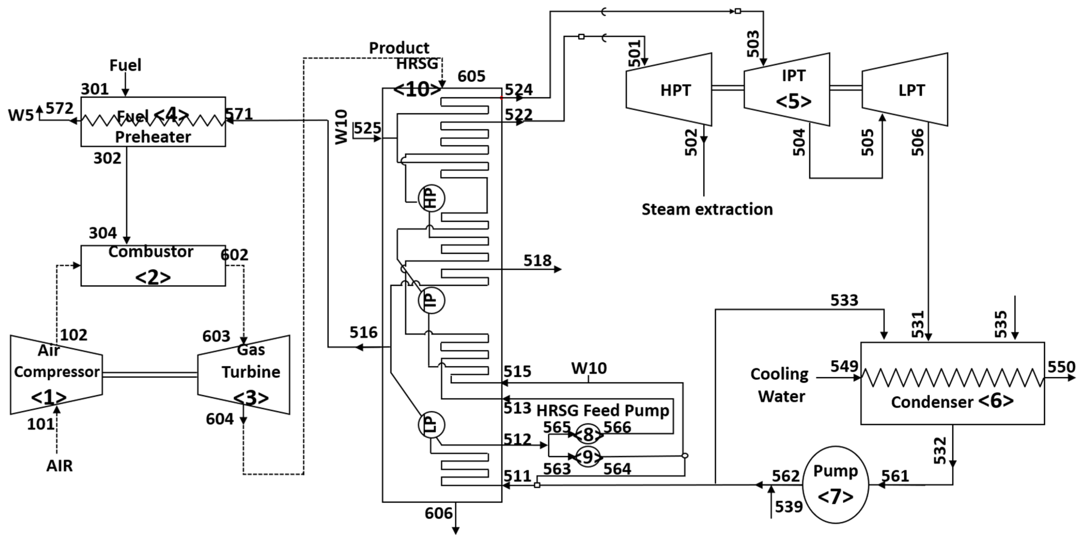
Figure 2.
Schematic of a 300 MW gas turbine cogeneration plant (HPR = 1.88).
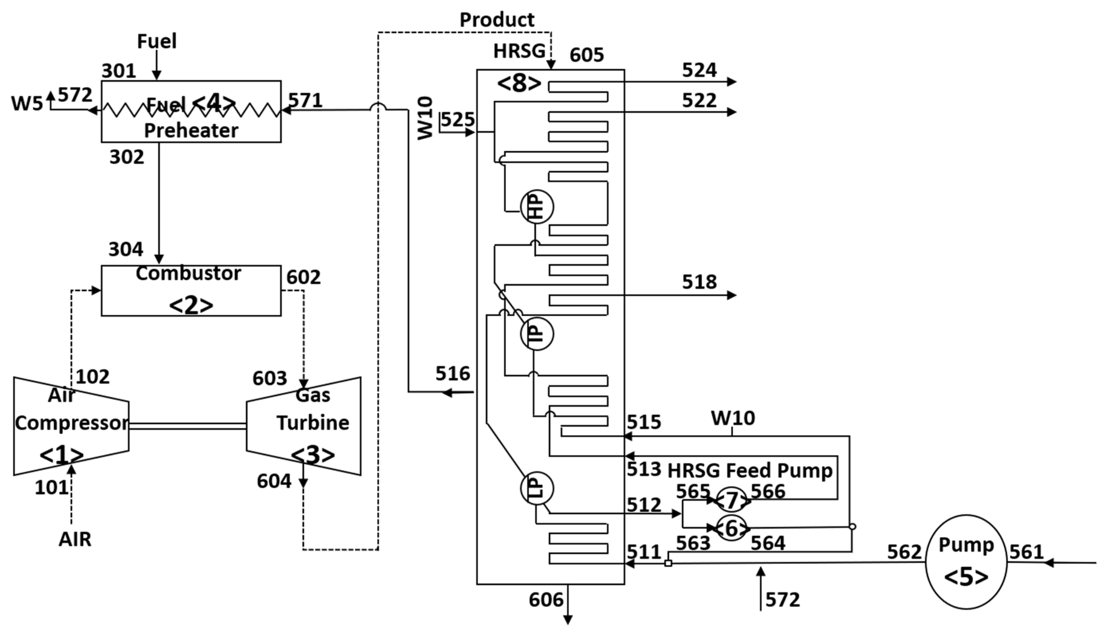
Figure 3.
Allocation of CO2 emissions to heat and electricity according to various allocation methods: (a) HPR = 0.59; (b) HPR = 1.88.
Figure 3.
Allocation of CO2 emissions to heat and electricity according to various allocation methods: (a) HPR = 0.59; (b) HPR = 1.88.
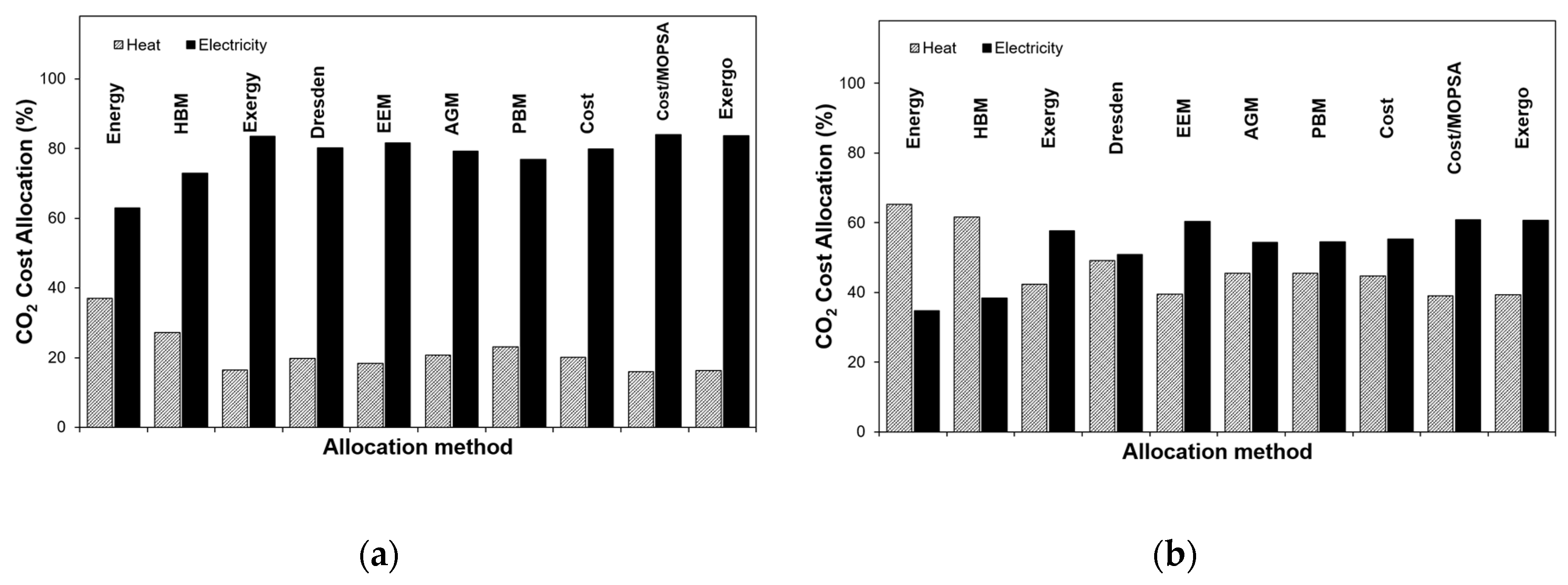
Figure 4.
Allocation ratios relative to the exergy method: (a) heat allocation ratio; (b) electricity allocation ratio.
Figure 4.
Allocation ratios relative to the exergy method: (a) heat allocation ratio; (b) electricity allocation ratio.
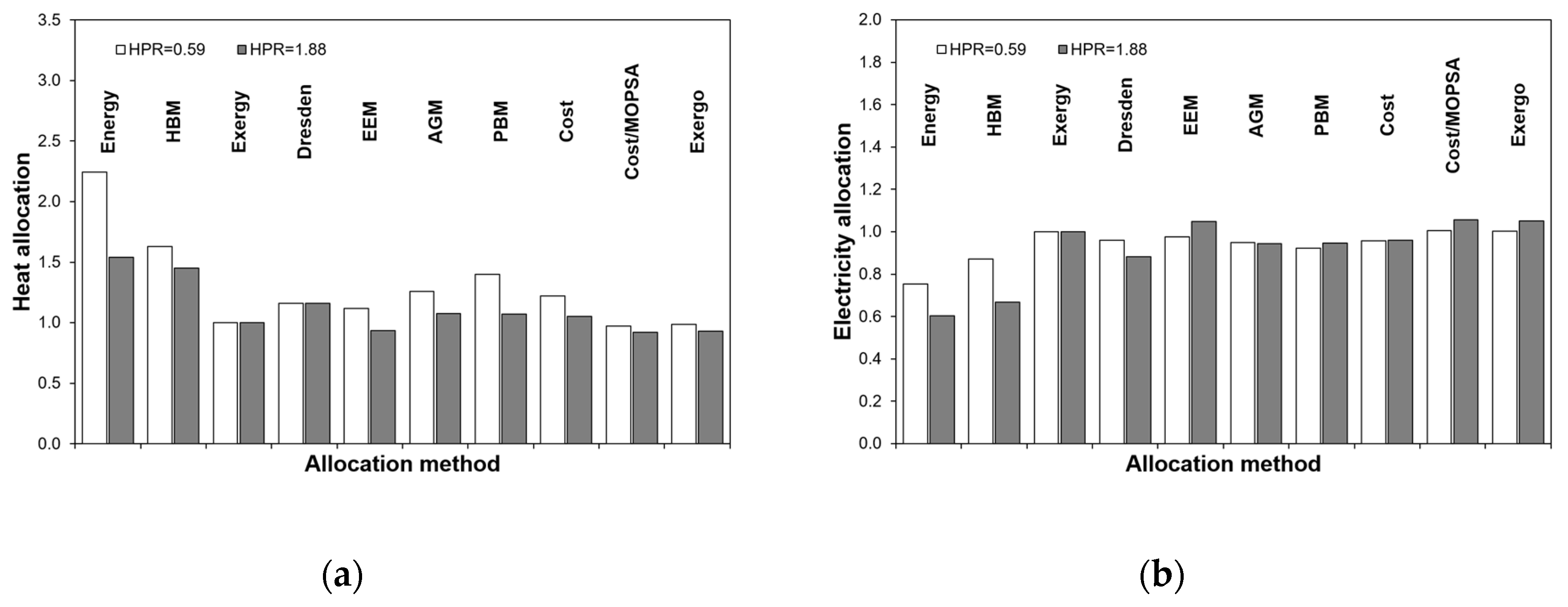
Figure 5.
Emission factors by various allocation methods for HPR values of 0.59 and 1.88: (a) heat emission factor; (b) electricity emission factor.
Figure 5.
Emission factors by various allocation methods for HPR values of 0.59 and 1.88: (a) heat emission factor; (b) electricity emission factor.
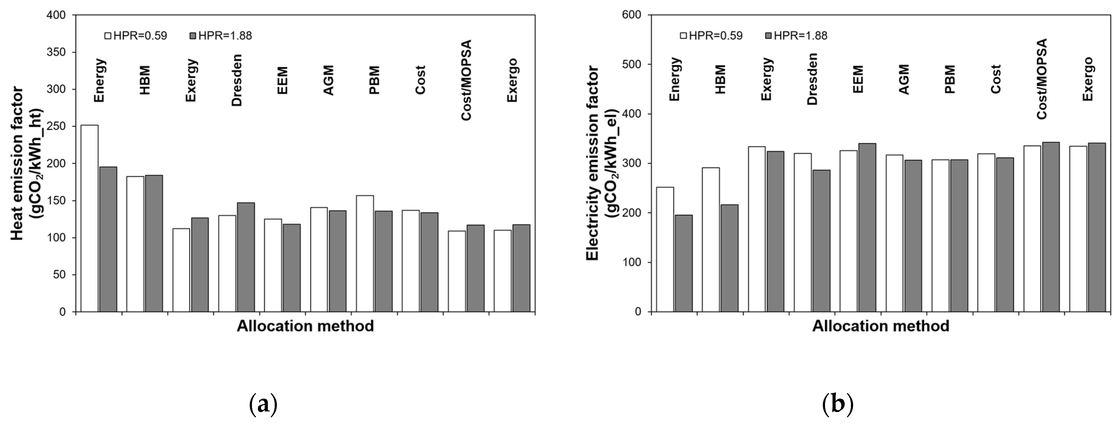
Table 2.
Exergy-balance equations for each component of the combined cycle cogeneration plant. The exergy destruction rate by Gouy-Stodola theorem for each component is shown in the third column.
Table 2.
Exergy-balance equations for each component of the combined cycle cogeneration plant. The exergy destruction rate by Gouy-Stodola theorem for each component is shown in the third column.
| Component | Exergy-balance equation | Exergy destruction |
|---|---|---|
| AC | ||
| COM | ||
| GT | ||
| FPH | ||
| ST | ||
| CON | ||
| CP | ||
| FPA | ||
| FPB | ||
| HRSG |
Table 3.
Cost-balance equations for each component of the combined cycle cogeneration plant.
| Component | Cost-balance equations |
|---|---|
| AC | |
| COM | |
| GT | |
| FPH | |
| ST | |
| CON | |
| CP | |
| FPA | |
| FPB | |
| HRSG | |
| T-Junction | |
| P-Junction | |
| DT-Junction | |
| DP-Junction | |
| W-Junction | |
| DW-Junction | |
| Boundary |
Table 4.
Various exergy flows for each component of the combined cycle cogeneration plant given in Figure 1.
Table 4.
Various exergy flows for each component of the combined cycle cogeneration plant given in Figure 1.
| Component |
(kW) |
(kW) |
(kW) |
Irreversibility rate (kW) | |
|---|---|---|---|---|---|
| AC | -285,940.0 | 82,025.4 | 169,982.3 | 22,460.1 | 11,472.1 |
| COM | -1,373,176.3* | 716,116.0 | 5513.3 | 306,164.9 | 345,382.1 |
| GT | 603,740.0 | -516,162.0 | -172,149.7 | -15,132.6 | 99,704.3 |
| FPH | -692.6 | 0.0 | 560.0 | 132.5 | |
| ST | 140,130.0 | -145,332.8 | -904.6 | -42,936.9 | 49,044.3 |
| COND | -14,579.7 | -472.7 | -22,172.2 | 37,224.7 | |
| PC | -11,901.5 | 8.1 | 391.7 | 10,698.9 | 802.8 |
| PFA | -210.2 | 19.5 | 156.9 | 12.9 | 21.0 |
| PFB | -2149.3 | 200.1 | 1599.2 | 135.1 | 214.9 |
| HRSG | -46,288.2 | -4024.3 | 35,467.6 | 14,845.0 | |
| Total | 443,669.0 (-1,373,176.3*) | 75,313.8 | 92.1 | 295,257.8 | 558,843.7 |
*Enthalpy of reaction at standard state.
Table 7.
Various exergy flows and irreversibility rate for each component of the gas turbine cogeneration plant given in Figure 2.
Table 7.
Various exergy flows and irreversibility rate for each component of the gas turbine cogeneration plant given in Figure 2.
| Component |
(kW) |
(kW) |
(kW) |
Irreversibility rate (kW) | |
|---|---|---|---|---|---|
| AC | -285,940.0 | 82,025.4 | 169,982.3 | 22,460.1 | 11,472.1 |
| COM | -1,373,176.3* | 709,999.1 | 0.0 | 304,940.9 | 358,236.4 |
| GT | 603,740.0 | -516,128.9 | -172,220.9 | -15,052.4 | 99,662.2 |
| FPH | 0.0 | -692.6 | 0.0 | 560.0 | 132.5 |
| PC | -671.2 | 0.2 | 347.1 | 256.8 | 67.1 |
| PFA | -236.5 | 19.5 | 156.9 | 12.9 | 47.3 |
| PFB | -2417.9 | 200.1 | 1599.2 | 135.0 | 483.6 |
| HRSG | -47,744.3 | -3957.4 | 39,541.0 | 12,160.7 | |
| Total | 314,474.4(-1,373,176.3*) | 227,678.5 | -4092.8 | 352,854.3 | 482,261.9 |
*Enthalpy of combustion at standard state.
Disclaimer/Publisher’s Note: The statements, opinions and data contained in all publications are solely those of the individual author(s) and contributor(s) and not of MDPI and/or the editor(s). MDPI and/or the editor(s) disclaim responsibility for any injury to people or property resulting from any ideas, methods, instructions or products referred to in the content. |
© 2026 by the authors. Licensee MDPI, Basel, Switzerland. This article is an open access article distributed under the terms and conditions of the Creative Commons Attribution (CC BY) license (http://creativecommons.org/licenses/by/4.0/).
Copyright: This open access article is published under a Creative Commons CC BY 4.0 license, which permit the free download, distribution, and reuse, provided that the author and preprint are cited in any reuse.