

Submitted:
10 November 2026
Posted:
12 November 2026
You are already at the latest version
Abstract
Degenerate horizons of black holes surrounded by a Kiselev quintessence fluid open into two product throats: a Nariai region dS2 × S2$ when the black-hole and cosmological horizons merge, and a Bertotti–Robinson region AdS2 × S2 when the charged hole becomes extremal. We study a scalar field on both throats in a family of time-dependent charts whose conformal factor is a difference of Weierstrass functions. These separable charts of constant curvature reduce the field equation to one Lamé equation read on two lines of a complex torus. On the Nariai throat, the occupation number between the conformal vacua at past and future infinity equals 1/sinh2 πσ for every mode and every chart, which we confirm to eight significant figures or better. On the Bertotti–Robinson throat, no normalizable mode is amplified, and the Floquet phase over one period of the chart is π times the sum of the conformal weight and the mode number. The fluid enters both results through one invariant: it lowers the temperature of the Nariai throat and moves the conformal weight of the Bertotti–Robinson throat off the integers. Particle numbers that depend on the chart appear only when the vacuum is fixed on a finite time slice, and we quantify them for adiabatic states of zeroth and second order.
Keywords:
particle creation
; Nariai throat
; Bertotti-Robinson throat
; quintessence
; Lamé equation
; adiabatic vacuum
1. Introduction
When two horizons of a static black hole coalesce, the region between them does not disappear. It opens into a throat whose geometry is a direct product of a two-dimensional constant-curvature spacetime and a round sphere of fixed radius. Merging a black-hole horizon with a cosmological horizon yields the Nariai geometry dS [1,2], while the extremal limit of a charged hole yields the Bertotti–Robinson geometry AdS [3,4]. Both throats are exact solutions in their own right, studied early on as backgrounds for quantum fields [5], and both appear as limits of wider families such as the C metric [6], charged dilaton holes [7] and black holes nucleated in de Sitter space [8]. Their quantum evolution [9], the tunneling picture of their radiation [10], and Schwinger pair production of charged quanta in them [11,12,13] have each been examined, and near-extremal throats now carry a sizable literature on quantum corrections to their thermodynamics [14] and on vacuum effects close to the horizon [15].
The two-dimensional factors of these throats are maximally symmetric, and that is where the quantum field theory becomes delicate. In de Sitter space the notion of a vacuum depends on the chart and on the boundary data used to define positive frequency [16,17,18,19]. The global in and out states differ [20,21], static and Poincaré patches carry their own preferred states [22,23,24], and different ways of distinguishing vacua in locally de Sitter cosmologies have been compared [25,26,27,28]. The anti-de Sitter side has its own version of the problem: on a Poincaré patch of AdS2, isometrically related observers disagree about particle content once mixed boundary conditions are imposed at the conformal boundary [29], and Bogoliubov transformations between AdS2 charts are tied to bulk reconstruction [30,31]. Exact pair-production rates for charged fields in dS2 and AdS2 are known in both global and planar charts [32], and they are related to each other by continuation of the curvature [33]. The symmetry structure behind these statements has been set out in Ref. [34], and particle creation by de Sitter black holes outside the throat limit has been studied as well [35,36].
Real black holes are rarely isolated, and a common way to model a surrounding dark-energy component is the Kiselev fluid [37], whose effect on null and timelike geodesics, on Hawking emission and on greybody factors has been worked out for neutral and charged holes [38,39]. Such a fluid changes where horizons merge and how large the resulting throat is. It is natural to ask how pair creation on the throat responds, and exact solutions of wave equations near horizons [40,41] suggest that the answer can be obtained in closed form. Two effects are easily conflated in such a calculation. One is the choice of chart, that is, which observers’ time is used to label the modes. The other is the choice of vacuum, that is, which boundary or initial data define the state. In many comparisons between de Sitter patches the chart and the state change together, and for quintessence-dressed throats the two effects have not been separated.
A recent analysis of adiabatic particle production in a time-dependent accelerated frame of flat spacetime, whose conformal factor is a sum of a function of time and a function of space, showed how far the state prepared at a symmetric instant departs from the inertial vacuum [42]. This paper carries the same structure to curved throats and makes the separation between chart and vacuum for both throats of a black hole in a Kiselev fluid. We use a family of time-dependent charts whose conformal factor is a difference of Weierstrass functions. These are separable charts of constant curvature of Liouville type [43]; their modulus interpolates between the global chart and charts in which the conformal factor depends on both coordinates, and in each of them the field equation reduces to a Lamé equation [44], an equation that has appeared before in parametric resonance after inflation [45]. We show that the particle content defined by conformal data is the same in every chart of the family, on both throats, and that the quintessence enters it through a single invariant. Chart dependence returns only when the state is fixed on a finite time slice. Section 2 derives the two throats and their invariants. Section 3 constructs the elliptic charts and the Lamé reduction. Section 4 and Section 5 treat the Nariai and Bertotti–Robinson throats, Sec. Section 6 turns to adiabatic states on a time-symmetric slice, and Sec. Section 7 concludes.
2. Throats of a Black Hole in a Kiselev Fluid
We work in units with signature and a sign convention in which de Sitter space has positive Ricci scalar. A static, spherically symmetric black hole carrying charge Q and surrounded by a Kiselev fluid with equation-of-state parameter has
where measures the fluid density [37,38]. The value is the one for which the fluid term is linear in r, which keeps the throat algebra closed. We consider two degenerate limits, each with one horizon radius at which .
The first limit is neutral, , with a positive cosmological constant. Solving the two conditions for the mass and for gives
For these reduce to and , the Nariai condition . Near the metric function is quadratic, , where is the small separation of the black-hole and cosmological horizons before the limit. The substitutions and followed by give [2,46]
This is dS in static coordinates. A positive and a real require . The fluid makes the de Sitter radius larger than the sphere radius, while in the pure Nariai case the two are equal.
The second limit has and nonzero charge. The degeneracy conditions now fix
which reduce to the extremal Reissner–Nordström values when . With and , the limit gives
which is AdS in Poincaré coordinates. A real charge and a real AdS radius require .
A scalar field of mass m coupled to curvature through obeys . On a product we write , and the four-dimensional equation becomes with
where on dS2 and on AdS2. Every result below depends on the field and on the fluid only through the dimensionless combination , where ℓ is the radius of the two-dimensional factor. Using Eqs. (3) and (5),
For a massless, minimally coupled field the two invariants are and . In both cases the fluid raises above its value for the bare throat. On the Bertotti–Robinson throat with the curvature term vanishes, because cancels the curvature of the sphere, so drops out entirely.
3. Elliptic Charts of Constant Curvature
Any two-dimensional metric can be written in conformal gauge, , and in the sign convention adopted here its scalar curvature is . The field equation then reads , and it separates in t and x whenever the conformal factor is a sum,
Metrics of this kind are of Liouville type. The task is to find all of them with constant curvature. Writing out for the sum (8) gives
and requiring this to equal is a polynomial identity once and are taken as polynomials in p and q. Matching coefficients shows that it holds when
for arbitrary constants . The flat case is ; it contains, for , and , the accelerated frame of Ref. [42]. For the functions p and q are affine images of the Weierstrass function , which satisfies with real roots and .
Let be the real half period and the imaginary one. On the real axis ℘ is real, has double poles at and , and is bounded below by ; on the shifted line it is real, regular, periodic with period , and confined to . Choosing and in Eq. (10) gives the two elliptic charts
which are positive everywhere because on the real line. We fix the unit of t and x by , so the charts form a one-parameter family labeled by the modulus . Figure 1 shows the conformal factor of both charts at . In the dS2 chart, F diverges on the lines and , which are past and future conformal infinity; in the AdS2 chart it diverges on the lines and , which are the two timelike boundaries. In the limit one finds on the real line while , so Eq. (11) tends to , the global chart of dS2 with conformal time , and Eq. (12) tends to , the global chart of AdS2. For the conformal factor depends on both coordinates, and the observers at fixed x follow a time-dependent family of trajectories. We confirmed numerically that equals and for the two charts at test points, to the accuracy of a centered finite difference, about .
Liouville’s general solution of the constant-curvature condition [43] makes the meaning of these charts precise. The general solution expresses F through two arbitrary monotonic functions and of the null coordinates and , and is the global metric written in the relabeled null coordinates . The elliptic charts are therefore global dS2 and AdS2 seen by a different family of observers. When the relabeling is smooth on the conformal boundary, as it is here, it multiplies a solution that behaves as a power of the distance to the boundary by a smooth function of the boundary coordinate, so each falloff class is preserved. Quantities fixed by falloff data at the conformal boundary must then come out the same in every chart, while quantities defined on a time slice need not. A relabeling that is singular on the boundary, such as the exponential map between Minkowski and Rindler null coordinates, does not have this property.
Separating in the dS2 chart with a constant gives
and in the AdS2 chart
In each case the time and space equations are the same Lamé equation [44], read on the real line and on the line shifted by . On dS2 the Lamé index satisfies , so for it is complex, with
On AdS2 it is real, , and we take the root . The modulus measures how far the chart is from the global one, and the problem is to find which properties of the field survive this deformation.
4. The Nariai Throat
The poles of at and fix the asymptotic form of every solution of the time equation in Eq. (13). Near a pole , because , so the local solutions behave as with , that is . Near the proper time of the throat is , and the factor oscillates with positive frequency . The in mode is therefore
where the bracket follows from inserting the Frobenius series into Eq. (13), and the prefactor fixes the Wronskian . With , the out mode is with , which oscillates with positive frequency in the proper time near future infinity and has the same Wronskian. The Bogoliubov coefficients of are
and they are evaluated from the solution that starts as Eq. (16) and is continued across the strip .
The allowed values of come from the spatial equation. A null ray const leaves past infinity and reaches future infinity after a spatial shift . In dS2 every null ray from past infinity crosses half of the spatial circle before reaching future infinity, so the circle has length , and the spatial equation must be solved with period . Its potential has period , so the physical are the union of the periodic and antiperiodic eigenvalues on , that is, the points where the trace of the spatial transfer matrix over one period equals . In the global limit the potential is constant, with , and Eq. (13) is the global mode equation with integer momentum on a circle of length .
We computed by integrating the time equation from the Frobenius data (16) at to with an eighth-order Runge–Kutta scheme at relative tolerance , the Weierstrass function being built from Jacobi elliptic functions. The physical were located as roots of the transfer-matrix trace and polished to . In the global limit the result is independent of and equals
the in/out mixing of the global chart, whose vacuum structure is discussed in Refs. [17,19,20]; this anchor was reproduced to seven significant figures or better for and . Table 1 reports the same calculation in elliptic charts with and , for the three lowest physical modes and three values of the invariant . In every case Eq. (18) holds, with relative deviations between and , and unitarity holds at the level of . The occupation number is the same in every chart of the family and for every mode, although the eigenvalues themselves move with .
The reason is the one anticipated in Sec. Section 3. The in and out states are defined by the exponents of the Frobenius solutions at conformal infinity, and these exponents are local invariants of the singular points of the Lamé equation, unchanged by any relabeling of the null coordinates that preserves the conformal boundary. The chart therefore cannot enter , and the whole dependence on the field, on the angular number and on the fluid sits in . Inserting Eq. (7),
For large , Eq. (19) behaves as with energy and
the Gibbons–Hawking temperature of the throat [47]. At fixed throat size the fluid cools the throat and, at the same time, raises the effective mass of every angular mode. Figure 2(a) shows the result for a massless, minimally coupled field. Between and the occupation of the mode falls from to , that of from to , and that of from to . Higher angular numbers are suppressed more strongly, because the fluid multiplies by before the square root is taken. Conformal coupling, , adds to and lowers the occupation at to .
5. The Bertotti–Robinson Throat
On the AdS2 throat the singular points of the Lamé equation lie on the boundaries and , and they control the spatial problem in Eq. (14). Near the solutions behave as and . For only the first is normalizable, and requiring at both boundaries fixes a discrete set , . Mixed boundary conditions, which would allow both falloffs, exist only in the window set by the Breitenlohner–Freedman bound [48]. For a massless field with one has , so the normalizable condition is the only one available. The exponent is the conformal weight of the mode,
which equals for a massless field on the bare throat.
The time equation in Eq. (14) has the periodic potential , and the chart oscillates forever. Whether a mode is amplified is decided by the trace of its transfer matrix over one period : for the mode grows exponentially, for it is quasi-periodic, and for it lies at a band edge. As a function of , the trace D has instability gaps where ; a scan of gives exactly n of them for , the finite-gap behavior expected of the Lamé equation with integer index, while for non-integer n new gaps keep appearing, with widths that shrink rapidly with (for the first three widths are , and ). We located the spatial eigenvalues by matching the normalizable Frobenius solutions from both boundaries at and then evaluated on the time line with the same integrator as before. Table 2 collects the results for two moduli and for invariants that give integer and non-integer n. In every case
to between and in absolute terms. Since , no normalizable mode is amplified, for any modulus and for any value of the fluid parameter. The instability gaps exist, but the spatial boundary conditions never place a physical inside one.
Equation (22) has a simple reading. The normal modes of global AdS2 with normalizable falloff have frequencies in global time [31], and a global-time interval multiplies the j-th mode by , whose trace in a real basis is . One period of the elliptic chart therefore advances every normalizable mode by exactly the phase that half a period of global time would produce, independently of the modulus. The particle content of the throat is again a property of the conformal boundary and not of the chart, and the statement agrees with the result of Ref. [29] that isometric observers on AdS2 agree about particles when the boundary condition is of Dirichlet or Neumann type.
The fluid enters only through . On the bare throat a massless field has integer weight ; the Floquet multipliers are then , and we verified that the full monodromy matrix equals to , so the evolution in the elliptic chart is strictly periodic, without secular growth. For the weight is generically irrational, and the evolution becomes quasi-periodic, with a rotation number set by the fractional part of . Integer weights return at the discrete values
for example and for , and and for . Figure 2(b) shows as a function of together with the integer levels. The quintessence fluid thus acts on the Bertotti–Robinson throat as a continuous shift of the conformal weight, and the dual statement on the Nariai throat is the shift of ; the two are related by the continuation of the Lamé index, in line with the dS2/AdS2 correspondence observed for charged pair production in Ref. [33].
6. Adiabatic States on a Time-Symmetric Slice
Section 4 and Section 5 show that states defined at conformal infinity or at the conformal boundary carry no memory of the chart. The chart becomes visible as soon as the state is fixed on a finite time slice. The natural slice of the dS2 elliptic chart is , where and the chart is symmetric under . With , the adiabatic vacuum of order at is defined, as in the flat accelerated frame of Ref. [42], by [49,50]
with at zeroth order. At second order the general expression reduces at the symmetric slice, where , to
where we used and . Evolving the data (24) to future infinity and projecting on gives the occupation of the out quanta in the adiabatic state.
Figure 3 shows and for the lowest physical mode as functions of the modulus, together with the conformal value (18). Three features stand out. First, the adiabatic occupations depend on : for on the bare throat, rises from at to at , and rises from to . They also depend on the mode within one chart; in the global limit, for instance, , and for , while the conformal value is for all three. Second, the zeroth-order state overshoots the conformal value by a factor of about six for and by more than two orders of magnitude for , where against . Third, the second-order state lies much closer to the conformal value but does not approach it monotonically in all modes: for it falls below the conformal value at small and crosses it near , and in the chart with the third physical mode has against . The adiabatic expansion is controlled by , and for the lowest angular numbers is of order a few, so higher adiabatic orders do not converge uniformly toward the conformal state.
These numbers make the separation between chart and vacuum explicit. Every difference between charts in Figure 3 comes from the instant at which the state was prepared and from the observers who prepared it. None of it survives when the same calculation is repeated with the conformal vacuum, which Table 1 shows to be the same in every chart. A statement that particle creation on a throat depends on the observer is therefore a statement about how the observer prepares the state.
7. Conclusions
We have studied a scalar field on the two throats of a black hole surrounded by a Kiselev quintessence fluid, the Nariai throat dS and the Bertotti–Robinson throat AdS, using a family of separable charts of constant curvature whose conformal factor is a difference of Weierstrass functions. In all of them the time and space equations are one Lamé equation read on two lines of a torus. On the Nariai throat the in/out occupation is for every mode and every chart, with , and the fluid acts by lowering the throat temperature to while raising the effective mass of each angular mode. On the Bertotti–Robinson throat no normalizable mode is amplified, the Floquet trace over one period of the chart is , and the fluid acts by moving the conformal weight off the integers, except at the discrete values of Eq. (23). What is universal is therefore the particle content defined by conformal data; what depends on the chart is the content of states prepared on a finite slice, which we have quantified for adiabatic vacua of zeroth and second order.
The global limits served as anchors. The elliptic charts reduce to the global charts as , where the Nariai occupation reproduces the global in/out value to seven significant figures or better for every integer momentum tested, and the throat parameters reduce to the Nariai condition and to extremal Reissner–Nordström when . The headline numbers were obtained by two independent routes, the analytic argument from the conformal exponents and direct integration with Frobenius boundary data, and these agree to at least eight significant figures on the Nariai throat and to twelve on the Bertotti–Robinson throat. The analysis concerns a test scalar field on the exact throats, with states fixed at conformal infinity, at the AdS2 boundary, or on the time-symmetric slice; it makes no claim about the black-hole exterior away from the degenerate limit, about backreaction, or about a flux reaching a distant observer.
In the near future, we plan to carry the analysis away from the exact throats by perturbing the Lamé equation in the horizon separation of a near-Nariai hole, where the maximal symmetry is broken at first order and the frame can enter the conformal particle number. In our next task agenda are also the Dirac and Maxwell fields on the same charts, whose Lamé indices are shifted by spin, and the fluid values of Eq. (23), where the integer weight suggests closed-form Lamé solutions for the adiabatic occupation.
Author Contributions
İ.S. conceived the study, derived the throat geometries and the elliptic-chart reduction to the Lamé equation, carried out the Bogoliubov, Floquet and adiabatic-vacuum computations with their independent checks, prepared the figures, wrote the manuscript via Overleaf, and approved its final version.
Data Availability Statement
The computational worksheets that support the findings of this study are available from the author upon reasonable request.
Use of Artificial Intelligence
During the preparation of this work, the author (İ.S.) used Writefull, integrated into the Overleaf editor, and the Overleaf AI assistant for English grammar and sentence-level language checking, the Google search engine for literature searches, and the built-in assistant in Maple 2024 to re-derive some algebraic results independently for verification. The author defined the research question, directed each step of the work, checked the derivations and the key numerical results by independent computation, and takes full responsibility for the content of this publication. The computational worksheets that reproduce the numerical results are available as Mathematica and Python notebooks from the author upon reasonable request.
Acknowledgments
İ.S. is grateful to EMU, TÜBİTAK, ANKOS and SCOAP3 for support and acknowledges the networking support of COST Actions CA18108, CA22113, CA21106, CA23130, CA23115, and CA21136.
References
- Nariai, H. On some static solutions of Einstein’s gravitational field equations in a spherically symmetric case. Sci. Rep. Tohoku Univ. 1950, 34, 160. [Google Scholar]
- Ginsparg, P.H.; Perry, M.J. Semiclassical perdurance of de Sitter space. Nucl. Phys. B 1983, 222, 245. [Google Scholar] [CrossRef]
- Bertotti, B. Uniform electromagnetic field in the theory of general relativity. Phys. Rev. 1959, 116, 1331. [Google Scholar] [CrossRef]
- Robinson, I. A solution of the Maxwell-Einstein equations. Bull. Acad. Pol. Sci. Ser. Sci. Math. Astron. Phys. 1959, 7, 351. [Google Scholar] [CrossRef]
- Villalba, V.M. Quantum effects associated with an electrically neutral massless particle in a Bertotti-Robinson universe. Mod. Phys. Lett. A 1994, 9, 3185–3191. [Google Scholar] [CrossRef]
- Dias, O.J.C.; Lemos, J.P.S. Extremal limits of the C metric: Nariai, Bertotti-Robinson, and anti-Nariai C metrics. Phys. Rev. D. 2003, 68, 104010. [Google Scholar] [CrossRef]
- Bousso, R. Charged Nariai black holes with a dilaton. Phys. Rev. D. 1997, 55, 3614–3621. [Google Scholar] [CrossRef]
- Bousso, R.; Hawking, S.W. Pair creation of black holes during inflation. Phys. Rev. D. 1996, 54, 6312. [Google Scholar] [CrossRef] [PubMed]
- Nojiri, S.; Odintsov, S.D. Quantum evolution of Schwarzschild-de Sitter (Nariai) black holes. Phys. Rev. D. 1999, 59, 044026. [Google Scholar] [CrossRef]
- Belgiorno, F.; Cacciatori, S.L.; Piazza, F.D. Tunneling method for Hawking radiation in the Nariai case. Gen. Relativ. Gravit. 2017, 49, 109. [Google Scholar] [CrossRef]
- Belgiorno, F.; Cacciatori, S.L.; Piazza, F.D. Pair-production of charged Dirac particles on charged Nariai and ultracold black hole manifolds. J. High Energy Phys. 2009, 08, 028. [Google Scholar] [CrossRef]
- Kim, S.P.; Lee, H.K.; Yoon, Y. Thermal interpretation of Schwinger effect in near-extremal RN black hole. Int. J. Mod. Phys. D. 2019, 28, 1950139. [Google Scholar] [CrossRef]
- Lin, P.; Shiu, G. Schwinger effect of extremal Reissner-Nordström black holes. J. High Energy Phys. 2025, 06, 17. [Google Scholar] [CrossRef]
- Banerjee, N.; Saha, M. Revisiting leading quantum corrections to near extremal black hole thermodynamics. J. High Energy Phys. 2023, 07, 10. [Google Scholar] [CrossRef]
- Hadi, H.; Akbarieh, A.R.; Esmer, G.D. Dynamical Casimir Effect and vacuum friction in the near-horizon geometry of a black hole. Phys. Lett. B 2026, 883, 141080. [Google Scholar] [CrossRef]
- Bunch, T.S.; Davies, P.C.W. Quantum field theory in de Sitter space: renormalization by point splitting. Proc. R. Soc. Lond. A 1978, 360, 117. [Google Scholar] [CrossRef]
- Mottola, E. Particle creation in de Sitter space. Phys. Rev. D. 1985, 31, 754. [Google Scholar] [CrossRef] [PubMed]
- Allen, B. Vacuum states in de Sitter space. Phys. Rev. D. 1985, 32, 3136. [Google Scholar] [CrossRef] [PubMed]
- Bousso, R.; Maloney, A.; Strominger, A. Conformal vacua and entropy in de Sitter space. Phys. Rev. D. 2002, 65, 104039. [Google Scholar] [CrossRef]
- Anderson, P.R.; Mottola, E. Instability of global de Sitter space to particle creation. Phys. Rev. D. 2014, 89, 104038. [Google Scholar] [CrossRef]
- Anderson, P.R.; Mottola, E.; Sanders, D.H. Decay of the de Sitter vacuum. Phys. Rev. D. 2018, 97, 065016. [Google Scholar] [CrossRef]
- Higuchi, A.; Yamamoto, K. Vacuum state in de Sitter spacetime with static charts. Phys. Rev. D. 2018, 98, 065014. [Google Scholar] [CrossRef]
- Akhmedov, E.T.; Moschella, U.; Popov, F.K. Characters of different secular effects in various patches of de Sitter space. Phys. Rev. D. 2019, 99, 086009. [Google Scholar] [CrossRef]
- Akhmedov, E.T.; Bazarov, V.K.; Diakonov, V.D.; Moschella, U. Quantum fields in the static de Sitter universe. Phys. Rev. D. 2020, 102, 085003. [Google Scholar] [CrossRef]
- Toussaint, V.; Louko, J. Vacua in locally de Sitter cosmologies, and how to distinguish them. Phys. Rev. D. 2024, 109, 025007. [Google Scholar] [CrossRef]
- Aslanbeigi, S.; Buck, M. A preferred ground state for the scalar field in de Sitter space. J. High Energy Phys. 2013, 08, 039. [Google Scholar] [CrossRef]
- Das, A.; Dalui, S.; Chowdhury, C.; Majhi, B.R. Conformal vacuum and the fluctuation-dissipation theorem in a de Sitter universe and black hole spacetimes. Phys. Rev. D. 2019, 100, 085002. [Google Scholar] [CrossRef]
- Tanhayi, M.R. Particle creation in global de Sitter space: Bulk space consideration. Int. J. Mod. Phys. D. 2015, 24, 1550052. [Google Scholar] [CrossRef]
- Pitelli, J.P.M.; Barroso, V.S. Particle production between isometric frames on a Poincare patch of AdS2. J. Math. Phys. 2019, 60, 092301. [Google Scholar] [CrossRef]
- Dey, P.; Kajuri, N. Bulk reconstruction and Bogoliubov transformations in AdS2. J. High Energy Phys. 2021, 09, 170. [Google Scholar] [CrossRef]
- Spradlin, M.; Strominger, A. Vacuum states for AdS(2) black holes. J. High Energy Phys. 1999, 11, 021. [Google Scholar] [CrossRef]
- Kim, S.P.; Page, D.N. Schwinger pair production in dS2 and AdS2. Phys. Rev. D. 2008, 78, 103517. [Google Scholar] [CrossRef]
- Chen, C.M.; Huang, C.C.; Kim, S.P.; Lin, K.Y. Reciprocal relation of Schwinger pair production between dS2 and AdS2. Phys. Rev. D. 2025, 112, 125028. [Google Scholar] [CrossRef]
- Epstein, H.; Moschella, U. QFT and Topology in Two Dimensions: SL(2, R)-Symmetry and the de Sitter Universe. Ann. Henri Poincaré 2021, 22, 2853–2891. [Google Scholar] [CrossRef]
- Bhattacharya, S. Particle creation by de Sitter black holes revisited. Phys. Rev. D. 2018, 98, 125013. [Google Scholar] [CrossRef]
- Bhattacharya, S.; Lahiri, A. Mass function and particle creation in Schwarzschild-de Sitter spacetime. Eur. Phys. J. C 2013, 73, 2673. [Google Scholar] [CrossRef]
- Kiselev, V.V. Quintessence and black holes. Class. Quantum Grav. 2003, 20, 1187. [Google Scholar] [CrossRef]
- Fernando, S.; Meadows, S.; Reis, K. Null Trajectories and Bending of Light in Charged Black Holes with Quintessence. Int. J. Theor. Phys. 2015, 54, 3634–3653. [Google Scholar] [CrossRef]
- Al-Badawi, A.; Kanzi, S.; Sakalli, I. Effect of quintessence on geodesics and Hawking radiation of Schwarzschild black hole. Eur. Phys. J. Plus 2020, 135, 219. [Google Scholar] [CrossRef]
- Sakalli, I. Analytical solutions in rotating linear dilaton black holes: Resonant frequencies, quantization, greybody factor, and Hawking radiation. Phys. Rev. D. 2016, 94, 084040. [Google Scholar] [CrossRef]
- Sakalli, I.; Al-Badawi, A. Exact solutions to a massive charged scalar field equation in the magnetically charged stringy black-hole geometry and Hawking radiation. Can. J. Phys. 2009, 87, 349–352. [Google Scholar] [CrossRef]
- Villalba, V.M. Adiabatic particle production in a time-dependent accelerated frame. arXiv 2026, arXiv:2610.18241. [Google Scholar] [CrossRef]
- Liouville, J. Sur l’équation aux différences partielles d2logλ/dudv±λ/2a2=0. J. Math. Pures Appl. 1853, 18, 71. [Google Scholar]
- Whittaker, E.T.; Watson, G.N. A Course of Modern Analysis, 4th ed.; Cambridge University Press: Cambridge, 1927. [Google Scholar]
- Greene, P.B.; Kofman, L.; Linde, A.D.; Starobinsky, A.A. Structure of resonance in preheating after inflation. Phys. Rev. D. 1997, 56, 6175. [Google Scholar] [CrossRef]
- Cardoso, V.; Lemos, J.P.S. Quasinormal modes of the near extremal Schwarzschild-de Sitter black hole. Phys. Rev. D. 2003, 67, 084020. [Google Scholar] [CrossRef]
- Gibbons, G.W.; Hawking, S.W. Cosmological event horizons, thermodynamics, and particle creation. Phys. Rev. D. 1977, 15, 2738. [Google Scholar] [CrossRef]
- Breitenlohner, P.; Freedman, D.Z. Stability in gauged extended supergravity. Ann. Phys. (N.Y.) 1982, 144, 249. [Google Scholar] [CrossRef]
- Parker, L. Quantized fields and particle creation in expanding universes. 1. Phys. Rev. 1969, 183, 1057. [Google Scholar] [CrossRef]
- Birrell, N.D.; Davies, P.C.W. Quantum Fields in Curved Space; Cambridge University Press: Cambridge, 1982. [Google Scholar] [CrossRef]
Figure 1.
Conformal factor of the elliptic charts at modulus . (a) The dS2 chart of Eq. (11): F diverges at and , the past and future conformal infinities, and is periodic in x with period ; the spatial circle has length . (b) The AdS2 chart of Eq. (12): F diverges at the two timelike boundaries and and oscillates in t with period .
Figure 1.
Conformal factor of the elliptic charts at modulus . (a) The dS2 chart of Eq. (11): F diverges at and , the past and future conformal infinities, and is periodic in x with period ; the spatial circle has length . (b) The AdS2 chart of Eq. (12): F diverges at the two timelike boundaries and and oscillates in t with period .
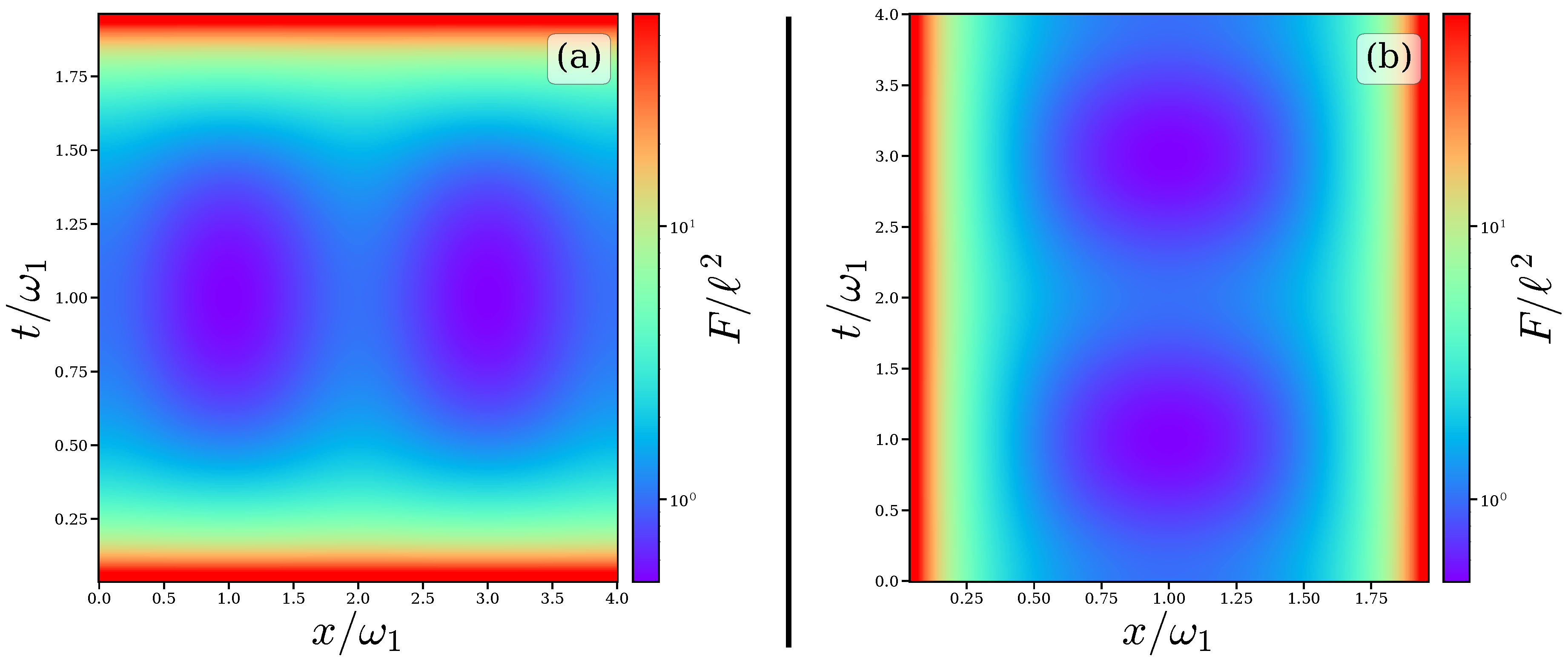
Figure 2.
Dependence of throat observables on the fluid parameter for a massless, minimally coupled field. (a) Occupation number (19) on the Nariai throat for ; the fluid lowers the throat temperature (20) and suppresses high angular numbers more strongly. (b) Conformal weight on the Bertotti–Robinson throat, Eq. (21); horizontal dotted lines mark integer weights, at which the evolution in the elliptic chart is strictly periodic.
Figure 2.
Dependence of throat observables on the fluid parameter for a massless, minimally coupled field. (a) Occupation number (19) on the Nariai throat for ; the fluid lowers the throat temperature (20) and suppresses high angular numbers more strongly. (b) Conformal weight on the Bertotti–Robinson throat, Eq. (21); horizontal dotted lines mark integer weights, at which the evolution in the elliptic chart is strictly periodic.
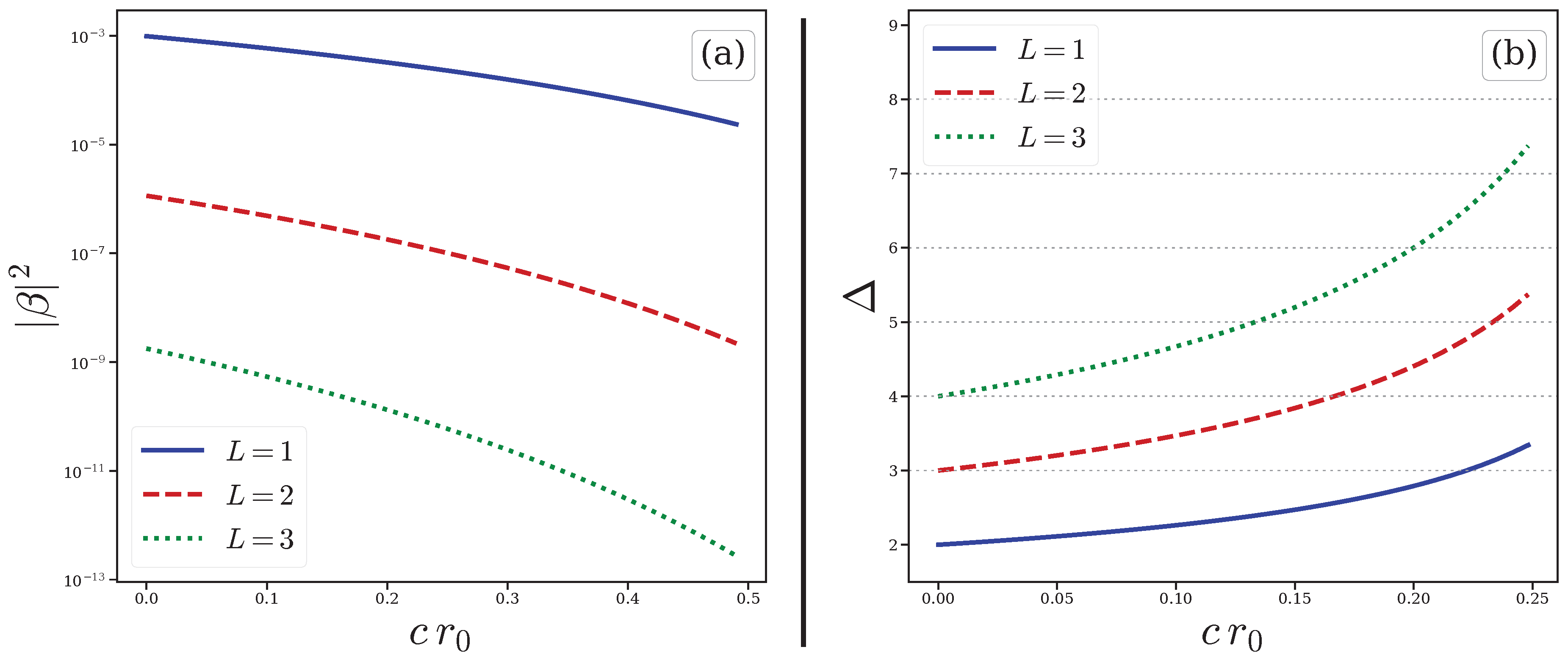
Figure 3.
Occupation at future infinity of the Nariai throat for the lowest physical mode prepared in the adiabatic vacuum of zeroth order, , and second order, , on the time-symmetric slice of the elliptic chart, as a function of the modulus . The dotted line is the chart-independent conformal value . (a) , (b) , both for a massless, minimally coupled field on the bare throat ().
Figure 3.
Occupation at future infinity of the Nariai throat for the lowest physical mode prepared in the adiabatic vacuum of zeroth order, , and second order, , on the time-symmetric slice of the elliptic chart, as a function of the modulus . The dotted line is the chart-independent conformal value . (a) , (b) , both for a massless, minimally coupled field on the bare throat ().
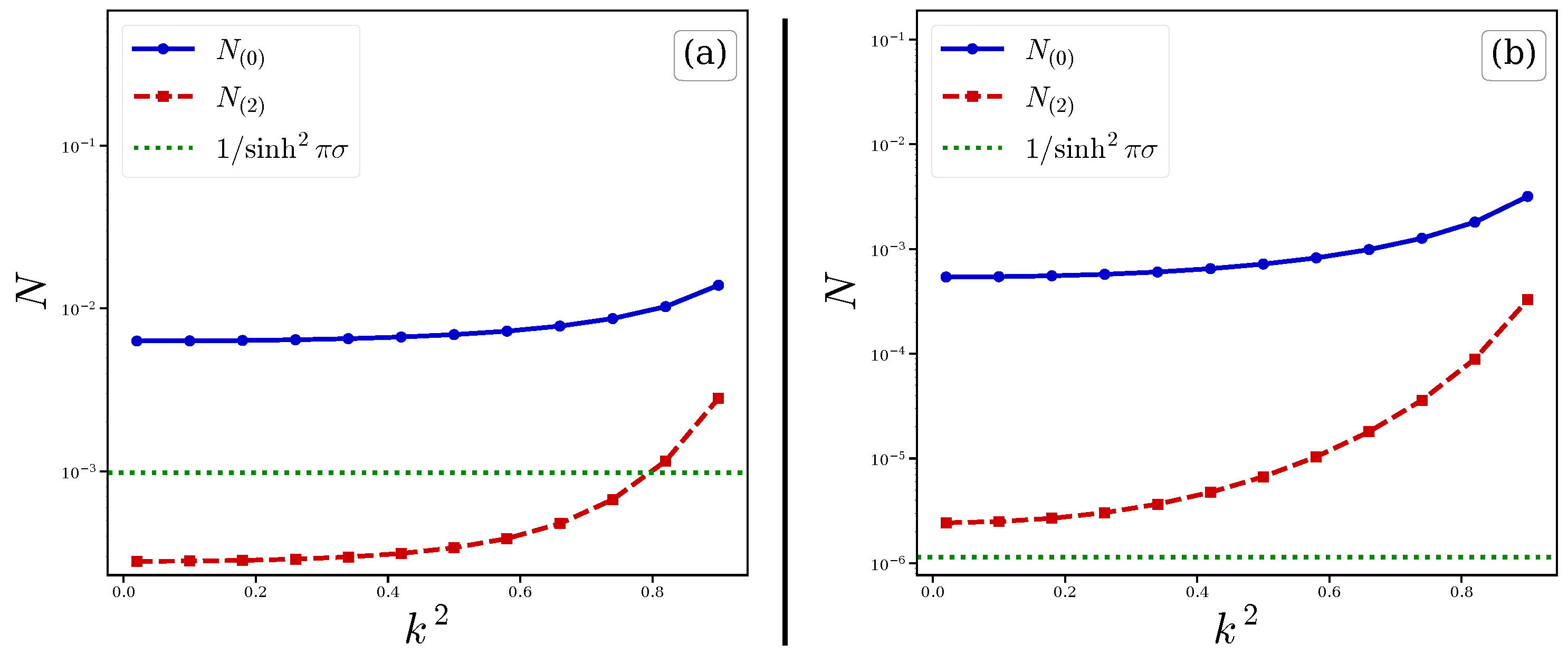

Table 1.
Occupation number between the conformal vacua at past and future infinity of the Nariai throat, computed in elliptic charts of modulus for the three lowest physical modes of the spatial circle. The last column gives the largest relative deviation from over the three modes. The field is massless and minimally coupled.
Table 1.
Occupation number between the conformal vacua at past and future infinity of the Nariai throat, computed in elliptic charts of modulus for the three lowest physical modes of the spatial circle. The last column gives the largest relative deviation from over the three modes. The field is massless and minimally coupled.
| L | |||||
|---|---|---|---|---|---|
| 1 | 0 | 2 | 0.3 | 0.5400, 1.2405, 1.5394 | |
| 1 | 0 | 2 | 0.7 | 0.2328, 0.5411, 1.2104 | |
| 2 | 0 | 6 | 0.3 | 1.5442, 2.0250, 2.9143 | |
| 2 | 0 | 6 | 0.7 | 0.3013, 0.3951, 2.2355 | |
| 1 | 0.3 | 2.8571 | 0.3 | 0.7635, 1.4104, 1.8367 | |
| 1 | 0.3 | 2.8571 | 0.7 | 0.2818, 0.5180, 1.4595 |
Table 2.
Transfer-matrix trace on the time line of the Bertotti–Robinson elliptic chart, evaluated at the three lowest normalizable spatial eigenvalues . The three traces agree in modulus with to the accuracy shown in the last column, and their signs alternate as , in accordance with Eq. (22). The field is massless and minimally coupled.
Table 2.
Transfer-matrix trace on the time line of the Bertotti–Robinson elliptic chart, evaluated at the three lowest normalizable spatial eigenvalues . The three traces agree in modulus with to the accuracy shown in the last column, and their signs alternate as , in accordance with Eq. (22). The field is massless and minimally coupled.
| L | ||||||
|---|---|---|---|---|---|---|
| 1 | 0 | 2 | 0.2 | 2.9907, 7.4686, 13.7391 | 2 | |
| 1 | 0 | 2 | 0.5 | 2.4284, 6.0084, 11.0303 | 2 | |
| 2 | 0 | 3 | 0.2 | 6.2854, 12.5532, 20.6143 | 2 | |
| 2 | 0 | 3 | 0.5 | 5.1373, 10.1393, 16.5896 | 2 | |
| 1 | 0.1 | 2.26271 | 0.2 | 3.7400, 8.6882, 15.4291 | 1.356637 | |
| 1 | 0.1 | 2.26271 | 0.5 | 3.0433, 6.9972, 12.3947 | 1.356637 | |
| 2 | 0.2 | 4.40512 | 0.2 | 12.9423, 21.7246, 32.3012 | 0.587331 | |
| 2 | 0.2 | 4.40512 | 0.5 | 10.6323, 17.6285, 26.0804 | 0.587331 |
Disclaimer/Publisher’s Note: The statements, opinions and data contained in all publications are solely those of the individual author(s) and contributor(s) and not of MDPI and/or the editor(s). MDPI and/or the editor(s) disclaim responsibility for any injury to people or property resulting from any ideas, methods, instructions or products referred to in the content. |
© 2026 by the authors. Licensee MDPI, Basel, Switzerland. This article is an open access article distributed under the terms and conditions of the Creative Commons Attribution (CC BY) license (http://creativecommons.org/licenses/by/4.0/).
Copyright: This open access article is published under a Creative Commons CC BY 4.0 license, which permit the free download, distribution, and reuse, provided that the author and preprint are cited in any reuse.