

Submitted:
10 November 2026
Posted:
12 November 2026
You are already at the latest version
Abstract
In the northern Peruvian highlands, milk production depends on ryegrass–white clover pastures that are rarely fertilised and used at long regrowth intervals. Two independent studies were conducted in 2024 at 3482 m a.s.l. Experiment 1 combined four balanced fertilisation levels (0–156 kg N ha−1 with macro- and micronutrients) and four cutting intervals (30–75 d) in a split-plot design over two cycles. In the rainy cycle, fertilisation raised yield per cut from 2216 (F0) to 4120 kg DM ha−1 (F2), with no gain at the highest rate. Daily productivity peaked at 60 d, but quadratic optima were imprecise. With 30- and 45-d cutting, third-cut yield fell to 53–57% of the first. Each additional regrowth day lowered crude protein by 0.11 and in vitro digestibility by 0.24 percentage points. With 60-d cutting, N and K2O removal exceeded inputs in every treatment. Experiment 2 compared two consecutive 12-day periods with the same 11 cows: traditional pasture and resown, fertilised pasture grazed at 42 d. In the second period, intake was 3.27 kg DM cow−1 d−1 higher, and milk yield 2.92 kg cow−1 d−1 higher (+30%), with unchanged milk composition. Because we did not replicate the order of the periods, we cannot attribute these differences solely to pasture management.
Keywords:
defoliation frequency
; nutrient balance
; compositional data
; Trifolium repens
; Lolium multiflorum
; milk yield
; blood metabolites
; high-Andean pastures
1. Introduction
Grasslands cover about one third of the Earth’s land surface [1,2]. Beyond forage, they support soil fertility and carbon storage and, when they include legumes, reduce the need for synthetic nitrogen [3,4]. High stocking rates and limited nutrient replacement accelerate their degradation [5], renewing interest in fertility programmes that address production and soil conservation together [6].
In the northern highlands of Peru, milk is the main source of rural income and is produced on mixed pastures of Lolium multiflorum L. ‘Cajamarca ecotype’ and Trifolium repens L. under extensive management, with yields close to 6 kg cow−1 d−1 [7]. Prevailing practice combines scarce fertilisation without soil analysis, use of the sward at the reproductive stage (60 d or more), white clover contents of 1 to 12.1% and intakes of 9.8 to 11.7 kg DM cow−1 d−1 [8]. As the forage frontier rises above 3500 m a.s.l., pastures are established on soils with very low pH and exchangeable aluminium [9,10], conditions that restrict root growth and fertiliser efficiency [11,12].
White clover supplies nitrogen through biological fixation and improves diet quality; in perennial ryegrass swards with about 31% clover, milk yield increased by 1.4 kg cow−1 d−1 [13,14,15]. Clover persistence depends on defoliation management and soil fertility [16,17]. Defoliation frequency affects both yield and nutritive value: longer intervals accumulate more biomass but with more fibre and lower protein and digestibility [18,19,20], whereas short intervals prevent replenishment of water-soluble carbohydrate reserves and compromise regrowth and persistence [21,22,23,24]. In temperate lowland environments, four- to six-week intervals are recommended for ryegrass–clover swards [17,25]; in the northern Peruvian highlands, farms use longer intervals [26].
The region has a rainy season (December to April) and a dry season (May to November), during which the mixture’s annual yield decreases by 18.74% [26] and its quality declines due to water deficit [27]. These variations can alter the diet’s energy-to-protein ratio and the cattle’s metabolic status, which blood profiles can assess [28,29], although dairy farmers in the region rarely use them.
Regional studies have examined phosphorus fertilisation and grazing frequency [30], as well as ryegrass and clover genotypes at different altitudes [9,10]. However, none has investigated the combined effects of macro- and micronutrient fertilisation and defoliation frequency on yield persistence, the balance between nutrient application and removal, or lactating cows’ response to a pasture-management package during the dry season. This paper presents two independent studies, each with a separate design and analysis. Experiment 1 aimed to quantify the effects of four levels of balanced fertilisation and four cutting intervals on the mixture’s yield, persistence, botanical composition, nutritive value, and nutrient balance. Experiment 2 aimed to compare grazing cows’ intake, milk yield and composition, and haematological and biochemical values between a period of traditional pasture management and a period involving resowing, NPK and micronutrient fertilisation, and use after 42 days of regrowth.
2. Materials and Methods
2.1. Study Site
Both studies were conducted in the hamlet of San Lorenzo, Calquis district, San Miguel province, Cajamarca region, Peru (6°52′49.52″ S; 78°55′3.52″ W; 3482 m a.s.l.). Mean temperatures range from 6.2 to 8 °C, relative humidity from 60 to 80%, and annual rainfall is 850 mm [26]. The experimental area held a seven-year-old mixed pasture with 49.4% ryegrass, 11.3% white clover and 39.3% weeds. The soil (0–20/30 cm) was a sandy loam with pH 4.73, 4.99% organic matter, 0.25% N, 20.48 mg kg−1 available P, 117.35 mg kg−1 available K and 2.55 cmol kg−1 Al3+. We determined organic matter by loss on ignition, pH by potentiometry in water, P by the modified Olsen method, and K, Ca, and Mg by extraction with ammonium acetate at pH 7 and atomic absorption spectroscopy (ISO 11260:2018).
2.2. Experiment 1: Balanced Fertilisation and Cutting Interval
2.2.1. Experimental Design and Treatments
A split-plot design in randomised complete blocks with three blocks was used. The main plot was fertilisation level (F0, no fertilisation; F1, low; F2, calculated from soil requirements; F3, high), and the 20 m2 subplot was cutting interval (30, 45, 60, and 75 d of regrowth). The area was resown with L. multiflorum ‘Cajamarca ecotype’ (35 kg ha−1; germination 73%, purity 78%) and T. repens cv. Huia (3 kg ha−1; germination 96%, purity 97%) on 20 February 2024. We harvested each subplot in three successive cuts, treated as repeated measures, across two evaluation cycles. In the first cycle (rainy season), the four-interval series started from a common standardisation cut (17 March 2024; first cuts on 16 April, 1 May, 16 May and 31 May 2024). In the second cycle (dry season), standardisation occurred between 28 June and 1 July 2024 (first cuts on 31 July, 12 August, and 29 August 2024), and the 75-d interval was not evaluated.
Fertilisation was split into two applications and included combined seabird guano, urea, triple superphosphate, potassium sulphate, sulpomag, dolomite, gypsum, and copper, zinc, and manganese sulphates, as well as ulexite (Table 1). Relative to F2, F1 and F3 deviated by −42% and +42% in N, −27% and +27% in P2O5 and −42% and +42% in K2O; Zn, Cu, Mn and B rates were the same in the three fertilised treatments, and dolomite was applied at a uniform rate to F1, F2 and F3 but not to F0.
2.2.2. Measurements
We measured herbage mass in two 0.25 m2 quadrats per subplot, cutting at 5 cm above ground level, and expressed it as kg DM ha−1. We measured plant height with a measuring tape in the stratum containing most leaves (70%). We calculated growth rate (GR) as yield divided by days to regrowth. We determined botanical composition by hand-separating each sample into ryegrass, white clover, Dactylis glomerata, and weeds, then expressing it as a percentage of dry weight. For nutritive value, composite samples were prepared by fertilisation level and interval (one per combination and cycle), dried at 65 °C for 48 h and analysed for crude protein (CP; AOAC 984.13), ash (AOAC 942.05) [31], neutral (NDF) and acid detergent fibre (ADF) [32] and in vitro DM digestibility (IVDMD) [33]. We determined concentrations of N, P2O5, K, Ca, Mg, Na, Zn, Fe, Cu, and Mn in one sample per subplot at 30, 60, and 75 d intervals (cycle 1) and at 30 and 60 d intervals (cycle 2).
2.2.3. Data Treatment
In the mineral analysis records, the sum of organic matter and ash equalled sample DM, indicating that N, organic matter, and ash were expressed on an air-dried basis (residual moisture 12 to 19%); we converted them to a dry basis by dividing by the DM fraction. We set a modified z-score threshold of |Mi| > 3.5 a priori as the criterion for implausible N concentrations [34]; this flagged three records (0.39%, 4.91% and 7.45% N on a dry basis), and we calculated the balance with and without them. We did not analyse the nutritive-value records of cycle 2 because their NDF (4–7%) and ash (22–34%) values are not plausible for this forage and indicate misassigned columns in the source records.
2.2.4. Statistical Analysis
We assessed yield transformation using the Box–Cox procedure on the full fixed-effects model for cycle 1 [35]. We analysed yield and GR on the log scale, so effects are expressed as ratios; because the 95% confidence interval (CI) of λ excluded zero, we repeated the analysis on the square-root and original scales, allowing residual variance to differ among intervals [36]. We analysed height on the original scale. For each cycle, a linear mixed model was fitted with fertilisation, interval, successive cut and their interactions as fixed effects, and block, main plot (block × fertilisation) and subplot (block × fertilisation × interval) as random effects [37]. We obtained the denominator degrees of freedom with the Kenward–Roger method [38,39]; in this balanced design, the F tests coincide with the classical analysis of variance by error strata. We compared the covariance among cuts within the same subplot under compound symmetry, first-order autoregressive (AR(1)), and unstructured models using AIC and BIC, and we calculated the Greenhouse–Geisser epsilon as a complement. Both cycles were combined in one model with the 30-, 45- and 60-d intervals (216 observations), with cycle as a fixed effect and a random subplot × cycle term. Because the cycle was not replicated across years, its effect confounds season, year, and the sward state at the end of the first cycle.
Means were back-transformed as exp(μ + σ2/2), where σ2 is the sum of the variance components of the model, and compared with Tukey’s test (α = 0.05) using the error stratum of each factor [40]. We expressed persistence as the ratio of third- to first-cut yield, with 95% CI, estimated from the corresponding contrast on the log scale.
We calculated productivity per unit time for each subplot as cumulative yield over three cuts divided by the days of occupation (three times the interval) and expressed it as an annual equivalent. For mean GR, digestible DM per day (GR × IVDMD), and CP per day (GR × CP), we fitted quadratic models of the cutting interval, with block as a fixed effect, using block-level data (n = 12) for each fertilisation level. We obtained the 95% CI of the vertex (−b1/2b2) using the delta method (normal approximation) and parametric bootstrap (5000 replicates) and compared the quadratic model with linear and linear-plateau models using AIC. Digestible DM and CP per day vary among blocks only through DM yield, because nutritive value comes from one composite sample per combination. In cycle 2, with three intervals, we estimated no optimum. The response to fertilisation intensity was modelled with the N rate as an index, in a quadratic model with block and interval as fixed effects (n = 48 subplots in cycle 1 and 36 in cycle 2), with and without F0.
We analysed botanical composition as compositional data [41]. D. glomerata was absent from 54.4% of the records, a structural zero, so it was analysed separately as presence/absence with a binomial generalised linear mixed model (fertilisation, cycle and their interaction as fixed effects, block as a random effect, Wald χ2 tests). The ryegrass–clover–weeds subcomposition was close to 100; we replaced the remaining zeros (1.3% of cells) multiplicatively with 0.65 times the minimum positive value in each part [42] and defined two isometric log-ratio balances [43]: ryegrass vs clover and sown species vs weeds. We analysed each balance using the mixed model described above; for reference, we report the analysis of raw percentages. We tested botanical structure using permutational multivariate analysis of variance on Aitchison distances [44,45], with 4999 permutations restricted to the design level: fertilisation on main-plot centroids with permutations within blocks, interval on subplot centroids with permutations within main plots, and cut on observations with permutations within subplots. We also tested homogeneity of multivariate dispersion.
We analysed the nutritive value in Cycle 1 using analysis of covariance, with regrowth days as a covariate and fertilisation as a factor, after verifying the homogeneity of slopes. We adjusted p-values using the false discovery rate (FDR) [46]. Because the samples were composites without block replication, the model error includes lack of fit; therefore, we do not present mean separations. We calculated CP and digestible DM yields per cut by multiplying each combination’s mean DM yield per cut by its CP or IVDMD concentration. We calculated nutrient removal by multiplying dry-basis concentration by the cumulative DM of the three cuts in the subplot for each cycle; K, Ca, and Mg were expressed as oxides (factors 1.2046, 1.3992, and 1.6583). We estimated the balance (supply − removal accumulated over the two cycles) for each block, with a t-based 95% CI and two degrees of freedom. With three blocks, resampling blocks yields only ten distinct samples and therefore was not used to calculate intervals. We present the initial and final soil analyses descriptively, each based on one composite sample.
Relative sustainability was summarised with TOPSIS [47,48] on seven criteria per fertilisation level: digestible DM per day and IVDMD (cycle 1), proportions of sown species and of weeds, N and K2O balances at 60 d, and persistence (mean of the cut 3/cut 1 ratio over all subplots of both cycles). Criteria were vector normalised. Three explicit weighting schemes (Table 9), 10,000 weight vectors drawn from a Dirichlet (1, …, 1) distribution and the 27 possible resamples of blocks were used to describe the stability of the ranking; with four alternatives, TOPSIS ranks but does not test differences. A principal component analysis (PCA) was performed on 14 standardised variables of the 16 fertilisation × interval combinations of cycle 1 (DM yield per cut, plant height, GR, height growth rate, CP, NDF, ADF, IVDMD, ash, CP yield per cut and the proportions of ryegrass, white clover, D. glomerata and weeds), followed by linear discriminant analysis on the first two or three components with leave-one-out cross-validation, Ward clustering with the number of groups chosen by mean silhouette width, and Pearson and Spearman correlations adjusted by FDR. All analyses were performed in R 4.3.3 [49] with the packages lme4, lmerTest, pbkrtest, nlme, emmeans, vegan and MASS; the scripts are provided as Supplementary Materials.
2.3. Experiment 2: Pasture Management and Response of Lactating Cows
2.3.1. Ethical Declarations
We declare that we conducted the present study in compliance with Law No. 30407, the Peruvian Animal Protection and Welfare Law, and international ethical standards for animal research. We implemented measures to minimise stress and avoid unnecessary suffering, ensuring proper handling in accordance with animal welfare principles. This included using appropriate restraint techniques and avoiding sudden movements during blood extraction from the coccygeal vein. Professional veterinary medical personnel trained at the Faculty of Veterinary Sciences of the National University of Cajamarca performed the procedure; additionally, the animal owners provided informed consent.
2.3.2. Animals, Pastures and Periods
The study used eleven Holstein and crossbred cows in the second third of lactation, with a mean live weight of 490 kg, a body condition score of 2.5, and two or more calvings; they grazed and were milked once daily (06:00 h) using a mechanical milking unit. The herd went through two consecutive 12-day periods. In T1 (16–27 July 2024), cows grazed the ryegrass–clover mixture under traditional management: fertilisation with poultry manure and use at 60 d of regrowth. In T2 (1–12 August 2024), they grazed the same mixture resown in November 2023 with ryegrass ‘Cajamarca ecotype’ and white clover cv. Huia, fertilised with NPK, manganese, copper, and zinc sulphates, and amendments (calcium hydroxide and calcium sulphate) according to the soil-test recommendation, was used at 42 d of regrowth. The botanical composition in T2 was 69% ryegrass, 22% clover, and 9% weeds. Four days elapsed between periods (28–31 July 2024). The treatments were not replicated, so the design compares two periods and cannot separate pasture management from date, stage of lactation, and weather.
2.3.3. Measurements
We estimated intake as the difference between herbage on offer and the residual, measured in 0.25 m2 quadrats and divided by the number of animals, with three determinations per period; we determined DM at 105 °C for 24 h. We analysed pasture nutritive value (three samples per period) at the Animal Nutrition and Food Bromatology Laboratory of the Universidad Nacional Toribio Rodríguez de Mendoza de Amazonas: CP (AOAC 984.13), ash (AOAC 942.05), NDF and ADF [32], and IVDMD using a DAISY incubator [50]. We estimated metabolizable energy (ME) as ME (MJ kg−1 DM) = 0.194 DOMD − 2.577, with DOMD = 0.84 IVDMD + 7.32 [51] and converted it to Mcal by dividing by 4.184.
Milk yield was recorded daily as herd yield divided by 11 cows (1 L ≈ 1 kg); no individual records were available. We determined fat, protein, milk urea nitrogen (MUN), and total solids in three samples per period using a MilkoScan™ 7 RM analyser (FOSS) at the Dairy Laboratory of the Universidad Nacional de Cajamarca. The fatty acid profile was determined in one milk sample per period (Société Générale de Surveillance, Lima; AOCS method Ce 1h-05). Energy-corrected milk (ECM), standardised to 4.0% fat and 3.3% protein, was calculated as kg milk × (0.383 F + 0.242 P + 0.7832)/3.1138, where F and P are the fat and protein percentages [52], and feed efficiency (FE) was calculated as ECM divided by DM intake [15].
At the end of each period, we sampled blood from the coccygeal vein of five cows after milking into EDTA tubes (5 mL) for haematology and plain tubes (7 mL) for biochemistry and analysed it at the Immunology and Research Laboratory of the Faculty of Veterinary Sciences, Universidad Nacional de Cajamarca. β-Hydroxybutyrate (BHB) was measured with test strips (BHBCHECK Plus). Erythrocyte indices were recalculated from red blood cell count (RBC), haemoglobin (Hb) and haematocrit (Hct): MCV = Hct/RBC × 10, MCH = Hb/RBC × 10 and MCHC = Hb/Hct × 100.
2.3.4. Statistical Analysis
Daily milk yield (n = 12 days per period) was analysed by generalised least squares with a first-order autoregressive structure between consecutive days within the period, compared by AIC with the model without autocorrelation; Welch’s t test, a permutation test (99,999 resamples) and a sensitivity analysis excluding 17 July 2024, a day with 5.45 kg cow−1, were also applied. For variables with n = 3 per period (intake, milk composition, and nutritive value), we used Welch’s t test, with an exact permutation test as a check (20 rearrangements; smallest attainable two-sided p = 0.10). For blood variables (n = 5 per period), we used Welch’s t test and an exact permutation test (252 rearrangements; minimum p = 0.008). Because we did not record the identity of the sampled cows, the main analysis treats them as independent samples; as a sensitivity analysis, we ran paired tests assuming row order identifies the same cow. Mean differences with 95% CI and Hedges’ g with approximate CI are reported [53]; p-values were adjusted by FDR within each family (milk composition; nutritive value; haematology, 12 variables; serum biochemistry, 17 variables). We also analysed the differential leukocyte count in centred log-ratio coordinates. We calculated ECM and FE from period means, and estimated their uncertainty by bootstrap, stratified by source (production days, composition samples, and intake samples; 10,000 replicates); we did not compute p-values. We present the fatty acid profile descriptively, with one sample per period.
3. Results
3.1. Experiment 1
3.1.1. Yield, Height and Growth Rate
The Box–Cox λ for cycle 1 yield was 0.42 (95% CI: 0.25–0.59). The log scale left residuals slightly non-normal (Shapiro–Wilk p = 0.040), whereas the square-root scale did not (p = 0.950); on all three scales, residual variance differed among intervals (Levene p ≤ 0.007). Fertilisation, interval, successive cut and the interval × cut interaction were significant on all three scales, with residual variance allowed to differ among intervals. The fertilisation × interval interaction depended on the scale: F (9,24) = 0.75 (p = 0.660) on the log scale, 2.57 (p = 0.031) on the square-root scale and 5.48 (p < 0.001) on the original scale. The fertilisation effect was therefore approximately proportional across intervals, but its absolute size increased with the cutting interval. The AR(1) structure among cuts had the lowest AIC (245.0 vs 248.3 for compound symmetry; φ = 0.35) and did not change the conclusions; the Greenhouse–Geisser epsilon was 0.79.

Table 2.
Analysis of variance of dry matter yield (log scale) and plant height by evaluation cycle.
| Cycle 1 (rainy) | Cycle 2 (dry) | |||||||||
| Source | df | DM, F | p | Height, F | p | df | DM, F | p | Height, F | p |
| Fertilisation (A) | 3, 6 | 25.14 | <0.001 | 41.13 | <0.001 | 3, 6 | 31.40 | <0.001 | 11.92 | 0.006 |
| Interval (B) | 3, 24 | 243.60 | <0.001 | 152.80 | <0.001 | 2, 16 | 93.81 | <0.001 | 305.63 | <0.001 |
| A × B | 9, 24 | 0.75 | 0.660 | 2.60 | 0.030 | 6, 16 | 0.84 | 0.560 | 0.97 | 0.475 |
| Cut (C) | 2, 64 | 26.51 | <0.001 | 0.03 | 0.975 | 2, 48 | 4.93 | 0.011 | 2.08 | 0.136 |
| A × C | 6, 64 | 1.05 | 0.405 | 0.66 | 0.680 | 6, 48 | 2.59 | 0.030 | 44.37 | <0.001 |
| B × C | 6, 64 | 12.22 | <0.001 | 2.35 | 0.041 | 4, 48 | 6.87 | <0.001 | 2.90 | 0.031 |
| A × B × C | 18, 64 | 1.03 | 0.440 | 1.13 | 0.348 | 12, 48 | 0.91 | 0.546 | 1.85 | 0.067 |
Linear mixed model with Kenward–Roger degrees of freedom. Cycle 1: 144 observations; cycle 2: 108 observations (75-d interval not evaluated). For height in cycle 1, the error-strata analysis gives F = 39.45 for fertilisation; the difference arises because the main-plot variance is estimated at the zero boundary.
In cycle 1, yield per cut increased from 2216 kg DM ha−1 in F0 to 4120 kg DM ha−1 in F2 (Table 3). The F2/F0 ratio was 1.86, and F3 did not differ from F2 or F1. Yields at 60 and 75 d did not differ (5600 and 5411 kg DM ha−1), but height was greater at 75 d. In cycle 2, F2 and F3 did not differ either (2024 and 2096 kg DM ha−1), and F2 did not differ from F1. Growth rate was highest at 60 d in both cycles; in cycle 2 it did not differ between 30 and 60 d (43.2 and 45.1 kg DM ha−1 d−1) and was lowest at 45 d.
3.1.2. Productivity per Unit Time and Cutting Interval
Normalised by days of occupation, cycle 1 productivity was highest at 60 d at all four fertilisation levels and declined at 75 d (Table 4); in F2 it fell from 44,890 to 32,146 kg DM ha−1 yr−1. Quadratic fits by fertilisation level placed the GR vertex at 63.6 d in F2 (95% CI, delta method: 42.0–85.2), that of digestible DM per day at 59.3 d (41.5–77.1) and that of CP per day at 57.5 d (37.9–77.2); in none of these fits was the quadratic term significant (p = 0.28–0.43), and the adjusted R2 did not exceed 0.17. In F1, the curve did not reach a maximum. With the four fertilisation levels in a single model, the vertex for digestible DM per day was at 63.6 d (48.3–78.8; p of the quadratic term = 0.10). In all cases, the linear-plateau model had an AIC lower than or similar to the quadratic model, with the break point at 60 d (62 d for GR in F1), which falls within the tested intervals. In both cycles, GR at 45 d was lower than at 30 d, a non-monotonic pattern that the quadratic model does not describe (Figure 1).
The GR response to N rate in cycle 1 was quadratic (b2 = −0.00212 ± 0.00058; p < 0.001; adjusted R2 = 0.80), with the vertex at 124.5 kg N ha−1 (95% CI, delta method: 95.9–153.1; parametric bootstrap: 104.7–181.8); for digestible DM per day, the vertex was at 124.8 kg N ha−1 (97.7–152.0). Without F0, the vertex was 116.4 kg N ha−1 (110.6–122.3), although with three rates the quadratic model reproduces the rate means exactly and its shape cannot be tested. In cycle 2, the quadratic term was not significant (p = 0.25), and the linear model had an equivalent AIC (235.8 vs 236.1), so there is no evidence of saturation up to 156 kg N ha−1, the highest rate tested.
3.1.3. Persistence of Yield Across Successive Cuts
The interval × cut interaction was significant in both cycles (Table 2). In cycle 1, third-cut yield was 53% of the first with 30-d cutting and 57% with 45-d cutting, whereas at 60 and 75 d it did not change (Table 5; Figure 2). In cycle 2, the ratios at 30 and 45 d did not differ from 1, and at 60 d the third cut exceeded the first by 33%.
3.1.4. Effect of Evaluation Cycle
In the combined model of the 30-, 45- and 60-d intervals, cycle affected yield (F1,24 = 148.30; p < 0.001): the arithmetic mean per cut fell from 3161 kg DM ha−1 in cycle 1 to 1837 kg DM ha−1 in cycle 2. The interval × cycle interaction was significant (F2,24 = 20.62; p < 0.001) because the advantage of the 60-d interval narrowed in cycle 2, as were the cut × cycle (F2,96 = 25.84; p < 0.001) and interval × cut × cycle (F4,96 = 8.11; p < 0.001) interactions. With the subplot × cycle error, the fertilisation × cycle interaction was not significant for yield (F (3,24) = 1.75; p = 0.183) but was significant for height (F (3,24) = 15.58; p < 0.001).
3.1.5. Botanical Composition
In cycle 1, fertilisation did not change either log-ratio balance: ryegrass vs clover, F (3,6) = 1.80 (p = 0.247), and sown species vs weeds, F (3,6) = 2.78 (p = 0.132). In the raw percentages, by contrast, fertilisation increased the proportion of ryegrass (F (3,6) = 16.14; p = 0.003) and reduced that of weeds (F (3,6) = 9.79; p = 0.010). The ryegrass–clover balance responded to interval (p < 0.001), cut (p < 0.001) and the fertilisation × interval (p = 0.004) and interval × cut (p < 0.001) interactions; the sown–weeds balance responded to cut (p = 0.009) and to the interval × cut interaction (p = 0.016). The proportion of clover fell from 13.8% at the first cut to 6.3% at the third, and that of weeds rose from 17.8% to 25.6% (Table 6). In cycle 2, fertilisation did not significantly affect the sown–weeds balance either (p = 0.072).
D. glomerata was present in 45.6% of the records. In cycle 2, its frequency of presence was 25.9% in F0, 37.0% in F1, 48.1% in F2 and 70.4% in F3, but neither fertilisation (χ2 = 4.97; df = 3; p = 0.174) nor its interaction with cycle (χ2 = 6.39; df = 3; p = 0.094) was significant.
In the permutational multivariate analysis, with permutations restricted at the main-plot level, fertilisation did not modify botanical structure (pseudo-F3,6 = 2.13; p = 0.096). Interval (pseudo-F3,24 = 3.97; p = 0.004), the fertilisation × interval interaction (pseudo-F9,24 = 2.25; p = 0.020), cut (pseudo-F2,88 = 5.73; p = 0.001) and the interval × cut interaction (pseudo-F6,88 = 3.59; p = 0.003) did. Each main factor explained 5.2- 6.9% of the total variation. Multivariate dispersion differed among fertilisation levels (p = 0.020) and intervals (p = 0.004), so part of the differences may reflect dispersion rather than location.
3.1.6. Nutritive Value and Nutrient Yields (Cycle 1)
Regrowth days were linearly associated with nutritive value, with no curvature (quadratic term p≥ 0.18) and homogeneous slopes across fertilisation levels (p ≥ 0.24) (Table 7). Fertilisation did not modify any variable after adjustment for regrowth days (adjusted p ≥ 0.46), including CP (F3,11 = 1.75; p = 0.215). CP yield per cut was highest at 60 d in F2 (885.5 kg ha−1); averaged over fertilisation levels, it was 280.1, 350.3, 779.5 and 667.6 kg ha−1 at 30, 45, 60 and 75 d, respectively, and digestible DM yield was 926.8, 1220.3, 2739.5 and 2564.1 kg ha−1.
3.1.7. Nutrient Balance
With 60-d cutting, cumulative removal over the two cycles exceeded N and K2O supply in all four treatments (Table 8). The largest N deficit corresponded to F2 (−1004 kg ha−1), the treatment with the highest DM yield; after excluding the three atypical N records, the F2 deficit was −969 kg ha−1, and that of F1 was −560 kg ha−1 (one block remaining). With 30-d cutting, the N balance was negative in all treatments, although the intervals for F2 and F3 included zero; had the supply in Table 1 been applied in each cycle, the N balance of F3 at 30 d would have been +27 kg ha−1 (95% CI: −124 to 177). The P2O5 balance was positive in F1, F2 and F3 at 30 d (13, 25 and 45 kg ha−1, respectively) and negative at 60 d; the MgO balance was positive in the fertilised treatments at both intervals. The horizons are not equivalent: six cuts at 30 d cover 180 days of regrowth, and six cuts at 60 d cover 360.
Between the start and end of the experiment, in one composite sample of the area, total soil N fell from 0.25 to 0.16%, available P from 20.5 to 9.7 mg kg−1, available K from 117.3 to 67.1 mg kg−1, organic matter from 4.99 to 3.24% and pH from 4.73 to 4.25.
3.1.8. Multicriteria Index
F3 had the highest index under all three weighting schemes (Table 9) and ranked first in 75.5% of the 10,000 random weight vectors and in 92.6% of the block resamples. F2 ranked second only under the productivity-oriented scheme (0.695 vs. 0.713 for F3) and last under the sustainability-oriented scheme (0.325).
Table 9.
Criteria, weights and TOPSIS index by fertilisation level.
| Criterion (direction) | Weights B/S/P | F0 | F1 | F2 | F3 |
| Digestible DM, kg ha−1 d−1 (+) | 0.14/0.10/0.35 | 24.6 | 32.8 | 43.0 | 37.4 |
| IVDMD, % (+) | 0.14/0.05/0.20 | 52.3 | 52.1 | 51.0 | 52.1 |
| Sown species, % (+) | 0.14/0.10/0.10 | 58.5 | 71.5 | 75.4 | 75.0 |
| Weeds, % (−) | 0.14/0.10/0.05 | 36.5 | 23.0 | 18.3 | 15.8 |
| N balance at 60 d, kg ha−1 (+) | 0.14/0.25/0.10 | −540 | −642 | −1004 | −516 |
| K2O balance at 60 d, kg ha−1 (+) | 0.14/0.20/0.10 | −646 | −594 | −891 | −808 |
| Persistence, cut 3/cut 1 (+) | 0.14/0.20/0.10 | 0.86 | 0.87 | 0.92 | 1.09 |
| Index, balanced scheme (B) | 0.413 | 0.640 | 0.530 | 0.785 | |
| Index, sustainability emphasis (S) | 0.608 | 0.680 | 0.325 | 0.775 | |
| Index, productivity emphasis (P) | 0.278 | 0.508 | 0.695 | 0.713 | |
| First rank with random weights (%) | 1.0 | 16.1 | 7.4 | 75.5 |
(+) benefit criterion; (−) cost criterion. Digestible DM and IVDMD: cycle 1; composition and persistence: both cycles. Balanced weights are 1/7 each. Random weights: Dirichlet (1, …, 1), 10,000 draws.
3.1.9. Multivariate Analysis and Correlations
The first two principal components of the 16 cycle-1 combinations explained 55.1% and 18.5% of the variation. The first contrasted DM yield, height, NDF, CP yield and ryegrass proportion with CP, IVDMD, ash and clover. Linear discriminant analysis on the first two components correctly classified 37.5% of the combinations by interval and 56.3% by fertilisation level (leave-one-out), against 25% expected by chance; with three components, 81.3% and 43.8%. Mean silhouette width was highest with two clusters (0.36). At the observation level, height was correlated with DM yield (r = 0.90, n = 144, in cycle 1; r = 0.65, n = 108, in cycle 2). Within each interval, correlations ranged from 0.55 to 0.81 in cycle 1 and from 0.02 to 0.34 in cycle 2. Across the 16 combinations of cycle 1, height was correlated with NDF (r = 0.84), IVDMD (r = −0.85) and CP (r = −0.87) (adjusted p < 0.001), but these correlations include the common effect of regrowth age.
3.2. Experiment 2
3.2.1. Intake and Milk Yield
Mean milk yield was 9.78 kg cow−1 d−1 in T1 and 12.71 kg cow−1 d−1 in T2 (Table 10; Figure 3). The model with AR(1) autocorrelation (φ = 0.39; AIC 81.8 vs. 82.7) estimated a difference of 2.92 kg cow−1 d−1 (95% CI: 1.35–4.50; p < 0.001), equivalent to +30% relative to T1. Excluding 17 July 2024, the difference was 2.61 kg cow−1 d−1 (1.62–3.60). During T1, yield increased by 0.34 kg cow−1 d−1 per day (p = 0.005); during T2, it did not change (0.07 kg cow−1 d−1 per day; p = 0.214). DM intake was higher in T2 by 3.27 kg cow−1 d−1 (+32.8% relative to T1; Welch’s t, p = 0.009); the exact permutation test gave p = 0.10, the smallest value attainable with three replicates per period.
3.2.2. Pasture Nutritive Value
Pasture CP was 2.65 percentage points higher in T2 (Table 11; adjusted p = 0.042). Ash was higher in T2 (p = 0.023), but not after adjustment (p = 0.068). NDF, ADF, IVDMD and ME did not differ; the 95% CIs of the differences spanned about ±16 percentage points for NDF and ±8 for IVDMD.
3.2.3. Fatty Acid Profile
With one sample per period, saturated fatty acids accounted for 60.1% of milk fat in T1 and 57.8% in T2; palmitic acid for 29.3% and 26.0%; and total trans fatty acids for 3.4% and 4.2%, respectively. Linolenic acid was 0.01 and 0.02 g per 100 g of milk. These values do not allow inferences between periods. The fat contents measured by SGS (4.06 and 3.84%) and by the MilkoScan analyser (3.96 and 4.16%) come from different samples and methods.
3.2.4. Haematology and Serum Biochemistry
After FDR adjustment, haematocrit was 9.66 percentage points higher in T2 (95% CI: 6.14–13.18; adjusted p = 0.017), and the proportion of eosinophils was 4.6 percentage points lower (95% CI: −7.0 to −2.2; adjusted p = 0.020) (Table 12). With adjusted permutation tests, RBC, Hb, Hct and eosinophils differed between periods (adjusted p = 0.024). In centred log-ratio coordinates, the share of eosinophils in the differential count was lower in T2 (adjusted p = 0.004), whereas those of monocytes and segmented neutrophils were higher (adjusted p = 0.010 and 0.025, respectively). Hb in T1 was exactly 0.33 times Hct in all five cows, indicating it was estimated from Hct rather than measured; comparisons of Hb, MCH, and MCHC are therefore not valid. In serum biochemistry, total protein, albumin, globulin, and calcium (higher in T2), and AST and magnesium (lower in T2), differed without adjustment (p = 0.004 to 0.049), but none did after adjustment (p ≥ 0.064). BHB did not differ (1.10 and 1.04 mmol L−1). In the paired sensitivity analysis, which assumes row order identifies the same cow, haematocrit, eosinophils, and magnesium were significant after adjustment (p = 0.026, 0.037, and 0.031, respectively).
All ten samples exceeded the upper limit of the laboratory reference range for GGT (17.4 U L−1) and for indirect bilirubin (<0.03 mg dL−1; observed range 0.14–0.30). The latter limit is incompatible with those given by the same source for total (0.01–0.5) and direct bilirubin (0.04–0.44). Values outside the laboratory ranges were also frequent for total protein (four of five cows below the lower limit in T1), albumin (four below in T1), globulin (four above in T2) and magnesium (all five above in T1 and one in T2); for the other variables with a stated range, at most two cows per period fell outside it.
4. Discussion
4.1. Experiment 1
4.1.1. Defoliation Interval
Productivity per unit time was higher with 60-d cutting than with any other interval at all four fertilisation levels in cycle 1, and it decreased when the interval was extended to 75 d. The data do not allow greater precision: with four intervals, a non-monotonic pattern between 30 and 45 d and a non-significant quadratic term, the estimated vertices (57 to 64 d in F2) have CIs more than 40 days wide, and the linear-plateau model, with its break at 60 d, fitted equally well or better. The recommendation is therefore limited to the tested 60-d interval; locating an optimum would require testing intermediate intervals (e.g., 50, 55, 65 and 70 d).
The most productive interval was twice that recommended for ryegrass–clover mixtures in temperate lowland environments [17,23,25]. A plausible explanation is that mean temperatures of 6 to 8 °C slow leaf appearance, so the same physiological stage is reached after more calendar days; this study did not measure phyllochron, leaves per tiller, or temperature during the trial, so the explanation remains a hypothesis. The observed intervals agree with those reported for the same mixture in the region [26].
4.1.2. Persistence
In cycle 1, third-cut yield was 53% and 57% of the first at 30- and 45-d intervals, whereas it was maintained at 60 and 75 d. This pattern is compatible with insufficient replenishment of soluble carbohydrates between frequent defoliations [21,23,24], but the design cannot separate it from the calendar. All series started from the same standardisation cut, so the three cuts at 30 d occurred between April and June, and those at 60 and 75 d in later and longer windows. The decline at 30 and 45 d may reflect plant depletion, the onset of the dry season or both. In cycle 2, with the same intervals, the ratio at 30 and 45 d did not differ from 1. Without the dates of each cut and without soil moisture records, depletion should be treated as a hypothesis.
4.1.3. Botanical Composition and White Clover
The proportion of clover declined between successive cuts (from 13.8% to 6.3% in cycle 1), while weeds increased from 17.8% to 25.6%. Clover therefore remained well below the sward contents of about 30% at which milk-yield responses have been reported [13,14]. The lowest clover value, at 75 d, is consistent with competition for light from ryegrass as it increased in height [16,54]. Fertilisation increased the proportion of ryegrass and reduced that of weeds in the percentage analysis, but did not change the log-ratio balances or the botanical structure when permutations respected the main plot (p = 0.096). With six degrees of freedom for the main-plot error and multivariate dispersion differing among levels, the evidence for an effect of fertilisation on composition is weak. The higher frequency of D. glomerata at high rates in cycle 2 was not statistically significant and cannot be interpreted as fertilisation-driven colonisation.
4.1.4. Response to Fertilisation Rate
In cycle 1, the response to fertilisation intensity was quadratic, peaking at 124.5 kg N ha−1 (95% CI: 96–153), close to the F2 rate (110 kg N ha−1). This is consistent with F3 not exceeding F2 despite receiving 46 kg N ha−1 more, and with the diminishing returns documented for forage grasses [55]. In cycle 2, we observed no curvature in the tested range, suggesting another factor limited growth, probably water or temperature, although neither was measured. Because N, P and K rates increased together from F1 to F3 and dolomite was applied only to the fertilised treatments, the N rate functions as an index of overall intensity: the effect cannot be attributed to N alone, and the contrast with F0 includes liming, which may be important in a soil with pH 4.73 and exchangeable aluminium [11,12].
4.1.5. Nutrient Balance
With 60-d cutting, N and K2O removal exceeded supply in all treatments, by 500 to 1000 kg ha−1 over both cycles, and the deficit was largest in the most productive treatment. In cutting systems, no nutrient return occurs through excreta, and K export is particularly high [56,57]. The decline in soil N, P, K, organic matter and pH between the start and end of the experiment is consistent with the calculation, but with one composite sample at each time, it cannot be attributed to particular treatments. The positive P2O5 balance at 30 d, together with the simultaneous decline in available P and pH, is compatible with P fixation by Al and Fe oxides in acid soils [58] and with acidification associated with urea nitrification [59]; the design cannot discriminate between these hypotheses. Two assumptions condition the size of the balances and remain to be confirmed: that N was expressed on an air-dried basis, and that the rates in Table 1 correspond to the whole experiment. If the rates were applied in each cycle, the deficits would decrease by the amount of supply, but the N balance at 60 d would remain negative in all four treatments.
4.1.6. Productivity Versus Sustainability
F2 had the highest mean yield, whereas F3 had the highest multicriteria index under the three weighting schemes, with random weights and in the block resamples. This difference depends partly on how the index is built: because removal increases with yield, the nutrient balance penalises the most productive treatment, and productivity enters the index both as a direct benefit and as a cost through the balance. The ranking does not indicate that fertilising above the agronomic optimum is advisable; it indicates that rates should match expected export, and that the N and K replacement needed with 60-d cutting exceeds any of the rates tested. An economic analysis, including fertiliser cost and milk price, is needed to make an operational recommendation.
4.1.7. Seasonality
The cycle reduced the mean yield per cut from 3161 to 1837 kg DM ha−1 and modified the response to the interval: in cycle 2, GR at 30 d equalled that at 60 d. Because the cycle was not repeated in another year, its effect combines season, year, and the sward state after the first cycle. Management recommendations should therefore be formulated by season [26,60].
4.1.8. Plant Height as a Field Criterion
Height was correlated with DM per cut (r = 0.90 in cycle 1), but much of this association reflects differences in regrowth age. Within a given interval, the correlation ranged from 0.55 to 0.81 in cycle 1 and from 0.02 to 0.34 in cycle 2. We estimated correlations with NDF and IVDMD for 16 combinations, which share the same interval effect. Before using height as a decision tool, season-specific calibration is required, as done for the rising plate meter [61].
4.1.9. Limitations
The experiment was conducted on one farm, for one year, with three blocks, leaving six degrees of freedom to test fertilisation. Interval and calendar window are partly confounded. We could not analyse the nutritive value of cycle 2, and cycle 1 comes from composite samples without replication. The soil analysis is descriptive. Estimates of digestible DM and CP per hectare indicate the potential for animal production, not intake or milk yield.
4.2. Experiment 2
4.2.1. Intake and Milk Yield
The period with resown pasture, fertilised with NPK and micronutrients and used at 42 d, coincided with an intake 3.27 kg DM cow−1 d−1 higher and a milk yield 2.92 kg cow−1 d−1 higher, as well as with pasture of higher CP (14.48 vs. 11.83%) and a higher clover proportion (22% vs. about 12%). These differences align with those reported for diets with more legume and less mature forage [15,51,62,63]. However, their magnitude cannot be attributed solely to pasture management. T1 and T2 were consecutive periods from the same herd, with the order not replicated and separated by four days, and milk yield increased by 0.34 kg cow−1 d−1 during T1. Part of the difference may reflect incomplete adaptation or a temporal trend preceding T2, in addition to differences in weather and lactation stage between July and August. We estimated intake from three determinations per period, and with that sample size, the permutation test cannot yield p < 0.10.
4.2.2. Milk Composition, ECM and Feed Efficiency
Fat, protein, total solids, and MUN did not differ between periods, with CIs that allow differences of up to 1.5 points in fat. MUN values (12.55 and 13.30 mg dL−1) were within the 12 to 15 mg dL−1 range established for maintaining performance [64]. ECM was 3.43 kg cow−1 d−1 higher in T2, mainly because of milk volume. FE was 0.97 and 0.99 kg ECM kg−1 DM, with a difference of 0.02 (95% CI: −0.13 to 0.16); the higher yield in T2 was associated with higher intake, without evidence of a change in efficiency [15].
4.2.3. Fatty Acid Profile
4.2.4. Blood Values
Haematocrit was higher in T2, and the eosinophil proportion was lower; both differences remained after adjustment and in the paired sensitivity analysis. The difference in RBC was significant only in the permutation tests, and the Hb difference cannot be interpreted because T1 Hb was estimated. Values in both periods remained within the ranges reported for grazing dairy cows [67,68]. With five animals per period, without individual identification and with the temporal confounding already described, these differences cannot be attributed to diet; they may also reflect hydration, handling stress, parasite status or variation between samplings. The lower eosinophil proportion may relate to parasite burden, but no coproparasitological analyses were performed.
Total protein, albumin, globulin and calcium were numerically higher in T2, and magnesium was lower, but no difference remained after adjustment. The relationship between dietary CP and serum proteins described in other studies [28,29] cannot be confirmed with the present sample size. BHB values (1.10 and 1.04 mmol L−1) did not differ. All cows exceeded the cited GGT limit, which could indicate hepatic involvement in an area endemic for Fasciola hepatica; however, without parasitological diagnosis and without a verified reference range, these data do not support this interpretation.
4.2.5. Limitations
The study lacks replication of treatment order and an adequate washout period. Milk yield was measured at herd level rather than per cow; intake and pasture quality were measured with three determinations per period, and the blood profile was measured in five unidentified cows. The estimated differences are therefore between management periods. A crossover design with groups of cows in both orders, and paddocks assigned simultaneously to both managements with individual records, would allow estimation of the effect of pasture management.
5. Conclusions
Experiment 1. In a ryegrass–clover mixture at 3482 m a.s.l., balanced fertilisation increased yield per cut up to F2 (110 kg N ha−1 with P, K, Ca, Mg, S and micronutrients), with no further gain in F3; in the favourable cycle, the response peaked near 125 kg N ha−1. Among the intervals tested, 60-d cutting gave the highest production per unit time and maintained yield across successive cuts, whereas with 30- and 45-d cutting third-cut yield was about half that of the first cut in cycle 1; the data do not allow a more precise optimum to be identified or the interval effect to be separated from the calendar. Each additional day of regrowth reduced CP by 0.11 and IVDMD by 0.24 percentage points. With 60-d cutting, none of the rates tested replaced the N and K removed, and soil N, P, K, organic matter, and pH declined, so fertiliser rates should be defined by expected export and season.
Experiment 2. The grazing period on the resown mixture, fertilised with NPK and micronutrients and used at 42 d, coincided with higher intake (+3.3 kg DM cow−1 d−1), higher milk yield (+2.9 kg cow−1 d−1) and higher pasture CP than the period under traditional management, with no change in milk composition or feed efficiency. Haematocrit was higher and the proportion of eosinophils lower in the second period; after correcting for multiple comparisons, the other blood variables did not differ. Because both management systems were applied in successive periods to the same herd, these differences cannot be attributed solely to pasture management and should be confirmed with a design that replicates treatment order.
Supplementary Materials
The following supporting information can be downloaded at the website of this paper posted on Preprints.org, Table S1: Ratios between fertilisation levels with 95% CI; Dataset S1: Original data of Experiments 1 and 2; Code S1: R scripts 00–06 reproducing all analyses, tables and figures.
Author Contributions
Conceptualization, L.V.-F., G.F.-I., M.A., R.V.-C., J.G. and W.A.-G.; methodology, L.V.-F., G.F.-I., M.A., R.V.-C., J.G. and W.A.-G.; formal analysis, L.V.-F., G.F.-I., M.A., R.V.-C., J.G. and W.A.-G.; investigation, H.H.-Y., A.D.-R., D.E. and C.P.M.; data curation, W.A.-G.; writing—original draft preparation, L.V.-F. and W.A.-G.; writing—review and editing, L.V.-F. and W.A.-G.; supervision, J.P.F., R.B.-C. and A.M.G.-B.; project administration, J.P.F., R.B.-C. and A.M.G.-B.; funding acquisition, J.P.F., R.B.-C. and A.M.G.-B. All authors have read and agreed to the published version of the manuscript.
Funding
This research was funded by the National University of Cajamarca. The APC was funded by the Vice-Rectorate for Research at the National University of Cajamarca.
Informed Consent Statement
Not applicable.
Data Availability Statement
The original data, the cleaned data and the R code used for all analyses are provided as Supplementary Materials.
Acknowledgments
The authors thank the researchers and livestock farmers who took part in the fieldwork, and the Universidad Nacional de Cajamarca for institutional support. We also thank Heber Eli Delgado Horna for the milk sample analyses and Greila Maidelith Rodríguez Fernández for collecting the milk and blood samples.
Conflicts of Interest
The authors declare no conflicts of interest.
References
- Reinermann, S.; Asam, S.; Kuenzer, C. Remote Sensing of Grassland Production and Management—A Review. Remote Sens. 2020, 12, 1949. [Google Scholar] [CrossRef]
- Stanciu, A.-Ș. Sustainable Forage Yield Improvement through Perennial Grass–Legume Intercropping in Degraded Grasslands. Turk. J. Agric. For. 2025, 49, 215–241. [Google Scholar] [CrossRef]
- Lüscher, A.; Mueller-Harvey, I.; Soussana, J.F.; Rees, R.M.; Peyraud, J.L. Potential of Legume-Based Grassland–Livestock Systems in Europe: A Review. Grass Forage Sci. 2014, 69, 206–228. [Google Scholar] [CrossRef] [PubMed]
- Martin, G.; Durand, J.-L.; Duru, M.; Gastal, F.; Julier, B.; Litrico, I.; Louarn, G.; Médiène, S.; Moreau, D.; Valentin-Morison, M.; et al. Role of Ley Pastures in Tomorrow’s Cropping Systems. A Review. Agron. Sustain. Dev. 2020, 40, 17. [Google Scholar] [CrossRef]
- Batista, P.H.D.; Almeida, G.L.P.; Silva, J.L.B.; Pandorfi, H.; Silva, M.V.; Silva, R.A.B.; Melo, M.V.N.; Lins, F.A.C.; Cordeiro Junior, J.J.F. Short-Term Grazing and Its Impacts on Soil and Pasture Degradation. DYNA 2020, 87, 123–128. [Google Scholar] [CrossRef]
- Silveira, M.L.; Kohmann, M.M. Maintaining Soil Fertility and Health for Sustainable Pastures. In Management Strategies for Sustainable Cattle Production in Southern Pastures; Rouquette, M., Jr., Aiken, G.E., Eds.; Academic Press: London, UK, 2020; pp. 35–58. [Google Scholar] [CrossRef]
- MIDAGRI. Anuario Estadístico: Producción Ganadera y Avícola 2021; Ministerio de Desarrollo Agrario y Riego: Lima, Peru, 2022. (In Spanish) [Google Scholar]
- Vallejos Fernández, L.A.; Rojas Guevara, I.B.; Perinango Gaitán, J.A.; Alcántara Mendoza, J. Vacas pastoreadas a estaca y su efecto sobre el consumo y condición de la pastura. UCV-Scientia (In Spanish) 2019, 11, 28–31. [Google Scholar] [CrossRef]
- Vallejos-Fernández, L.A.; Alvarez, W.Y.; Paredes-Arana, M.E.; Pinares-Patiño, C.; Bustíos-Valdivia, J.C.; Vásquez, H.; García-Ticllacuri, R. Comportamiento productivo y valor nutricional de 22 genotipos de raigrás (Lolium spp.) en tres pisos altoandinos del norte de Perú. Sci. Agropecu. (In Spanish) 2020, 11, 537–545. [Google Scholar] [CrossRef]
- Vallejos Fernández, L.A.; Alvarez García, W.Y.; Paredes Arana, M.; Saldanha Odriozola, S.; Guillén-Sanchez, R.; Pinares Patiño, C.; Bustíos Valdivia, J.; García Ticllacuri, R. Comportamiento productivo y valor nutricional de siete genotipos de trébol en tres pisos altitudinales de la sierra norte del Perú. Rev. Investig. Vet. Perú (In Spanish) 2021, 32, e17690. [Google Scholar] [CrossRef]
- Kochian, L.V.; Piñeros, M.A.; Liu, J.; Magalhaes, J.V. Plant Adaptation to Acid Soils: The Molecular Basis for Crop Aluminum Resistance. Annu. Rev. Plant Biol. 2015, 66, 571–598. [Google Scholar] [CrossRef] [PubMed]
- Shetty, R.; Vidya, C.S.N.; Prakash, N.B.; Lux, A.; Vaculík, M. Aluminum Toxicity in Plants and Its Possible Mitigation in Acid Soils by Biochar: A Review. Sci. Total Environ. 2021, 765, 142744. [Google Scholar] [CrossRef] [PubMed]
- Dineen, M.; Delaby, L.; Gilliland, T.; McCarthy, B. Meta-Analysis of the Effect of White Clover Inclusion in Perennial Ryegrass Swards on Milk Production. J. Dairy Sci. 2018, 101, 1804–1816. [Google Scholar] [CrossRef] [PubMed]
- Egan, M.; Galvin, N.; Hennessy, D. Incorporating White Clover (Trifolium repens L.) into Perennial Ryegrass (Lolium perenne L.) Swards Receiving Varying Levels of Nitrogen Fertilizer: Effects on Milk and Herbage Production. J. Dairy Sci. 2018, 101, 3412–3427. [Google Scholar] [CrossRef] [PubMed]
- Johansen, M.; Lund, P.; Weisbjerg, M.R. Feed Intake and Milk Production in Dairy Cows Fed Different Grass and Legume Species: A Meta-Analysis. Animal 2018, 12, 66–75. [Google Scholar] [CrossRef] [PubMed]
- Enriquez-Hidalgo, D.; Gilliland, T.J.; Egan, M.; Hennessy, D. Production and Quality Benefits of White Clover Inclusion into Ryegrass Swards at Different Nitrogen Fertilizer Rates. J. Agric. Sci. 2018, 156, 378–386. [Google Scholar] [CrossRef]
- Phelan, P.; Casey, I.A.; Humphreys, J. The Effect of Target Postgrazing Height on Sward Clover Content, Herbage Yield, and Dairy Production from Grass–White Clover Pasture. J. Dairy Sci. 2013, 96, 1598–1611. [Google Scholar] [CrossRef] [PubMed]
- Gierus, M.; Kleen, J.; Loges, R.; Taube, F. Forage Legume Species Determine the Nutritional Quality of Binary Mixtures with Perennial Ryegrass in the First Production Year. Anim. Feed Sci. Technol. 2012, 172, 150–161. [Google Scholar] [CrossRef]
- Komainda, M.; Isselstein, J. Effects of Functional Traits of Perennial Ryegrass Cultivars on Forage Quality in Mixtures and Pure Stands. J. Agric. Sci. 2020, 158, 173–184. [Google Scholar] [CrossRef]
- Tilus, G.; Zinn, R.A.; Joseph, M.; Chay-Canul, A.J.; Santillano-Cazares, J.; Galicia-Juarez, M.; Tilus, M.L.; Tilus, D.; Estrada-Delgado, E.E.; Montaño-Gomez, M.F. Forage Yield, Elongation Rate and Botanical Composition of Lolium multiflorum Lamb. in Response to Different Grazing Intervals and Intensities. Trop. Subtrop. Agroecosyst. 2022, 25, 063. [Google Scholar] [CrossRef]
- Donaghy, D.J.; Fulkerson, W.J. Priority for Allocation of Water-Soluble Carbohydrate Reserves during Regrowth of Lolium perenne. Grass Forage Sci. 1998, 53, 211–218. [Google Scholar] [CrossRef]
- Fulkerson, W.J.; Donaghy, D.J. Plant-Soluble Carbohydrate Reserves and Senescence—Key Criteria for Developing an Effective Grazing Management System for Ryegrass-Based Pastures: A Review. Aust. J. Exp. Agric. 2001, 41, 261–275. [Google Scholar] [CrossRef]
- Turner, L.R.; Donaghy, D.J.; Lane, P.A.; Rawnsley, R.P. Effect of Defoliation Management, Based on Leaf Stage, on Perennial Ryegrass (Lolium perenne L.), Prairie Grass (Bromus willdenowii Kunth.) and Cocksfoot (Dactylis glomerata L.) under Dryland Conditions. 1. Regrowth, Tillering and Water-Soluble Carbohydrate Concentration. Grass Forage Sci. 2006, 61, 164–174. [Google Scholar] [CrossRef]
- Tozer, K.N.; Greenfield, R.M.; Cameron, C.A.; Upsdell, M.P.; Hume, D.E. Effect of Three Defoliation Frequency Treatments and Drought on Perennial Ryegrass Herbage and Root Growth and Water-Soluble Carbohydrate Reserves. Grassl. Res. 2024, 3, 347–363. [Google Scholar] [CrossRef]
- Acharán, F.A.; Balocchi, O.A.; López, I.F. Filocrono, producción de fitomasa y calidad nutritiva de una pradera de Lolium perenne L./Trifolium repens L. sometida a tres frecuencias e intensidades de defoliación. Agro Sur (In Spanish) 2009, 37, 81–90. [Google Scholar] [CrossRef]
- Vallejos-Cacho, R.; Vallejos-Fernández, L.A.; Alvarez-García, W.Y.; Tapia-Acosta, E.A.; Saldanha-Odriozola, S.; Quilcate-Pairazaman, C.E. Sustainability of Lolium multiflorum L. ‘Cajamarquino Ecotype’, Associated with Trifolium repens L., at Three Cutting Frequencies in the Northern Highlands of Peru. Sustainability 2024, 16, 6927. [Google Scholar] [CrossRef]
- Melo, C.D.; Maduro Dias, C.S.A.M.; Wallon, S.; Borba, A.E.S.; Madruga, J.; Borges, P.A.V.; Ferreira, M.T.; Elias, R.B. Influence of Climate Variability and Soil Fertility on the Forage Quality and Productivity in Azorean Pastures. Agriculture 2022, 12, 358. [Google Scholar] [CrossRef]
- Quinteros, O.R.; Vargas, J.C.; Barbona, I.; Marini, P.R. Indicadores metabólicos sanguíneos de genotipos lecheros en pastoreo de la provincia de Napo-Ecuador. La. Granja (In Spanish) 2017, 26, 119–130. [Google Scholar] [CrossRef]
- Maurya, S.K.; Singh, O.P. Blood Biochemical Profile and Nutritional Status of Dairy Cows under Field Conditions. J. Anim. Res. 2016, 6, 167–170. [Google Scholar] [CrossRef]
- Vallejos, L. Efecto de la Fertilización Fosforada y Frecuencia de Pastoreo sobre el Valor Nutritivo de la Dieta y Comportamiento Ingestivo de las Vacas Holstein en Pasturas de Ryegrass–Trébol en Cajamarca. Ph.D. Thesis, (In Spanish) Universidad Nacional Agraria La Molina, Lima, Peru, 2009. [Google Scholar]
- AOAC International. Official Methods of Analysis of AOAC International, 19th ed.; AOAC International: Gaithersburg, MD, USA, 2012. [Google Scholar]
- Van Soest, P.J.; Robertson, J.B.; Lewis, B.A. Methods for Dietary Fiber, Neutral Detergent Fiber, and Nonstarch Polysaccharides in Relation to Animal Nutrition. J. Dairy Sci. 1991, 74, 3583–3597. [Google Scholar] [CrossRef] [PubMed]
- Tilley, J.M.A.; Terry, R.A. A Two-Stage Technique for the In Vitro Digestion of Forage Crops. J. Br. Grassl. Soc. 1963, 18, 104–111. [Google Scholar] [CrossRef]
- Iglewicz, B.; Hoaglin, D.C. How to Detect and Handle Outliers; ASQC Quality Press: Milwaukee, WI, USA, 1993. [Google Scholar]
- Box, G.E.P.; Cox, D.R. An Analysis of Transformations. J. R. Stat. Soc. Ser. B 1964, 26, 211–252. [Google Scholar] [CrossRef]
- Pinheiro, J.C.; Bates, D.M. Mixed-Effects Models in S and S-PLUS; Springer: New York, NY, USA, 2000. [Google Scholar] [CrossRef]
- Bates, D.; Mächler, M.; Bolker, B.; Walker, S. Fitting Linear Mixed-Effects Models Using lme4. J. Stat. Softw. 2015, 67, 1–48. [Google Scholar] [CrossRef]
- Kenward, M.G.; Roger, J.H. Small Sample Inference for Fixed Effects from Restricted Maximum Likelihood. Biometrics 1997, 53, 983–997. [Google Scholar] [CrossRef]
- Kuznetsova, A.; Brockhoff, P.B.; Christensen, R.H.B. lmerTest Package: Tests in Linear Mixed Effects Models. J. Stat. Softw. 2017, 82, 1–26. [Google Scholar] [CrossRef]
- Lenth, R.V. emmeans: Estimated Marginal Means, aka Least-Squares Means, R Package Version 1.10.0. 2024. Available online: https://CRAN.R-project.org/package=emmeans (accessed on [fecha]).
- Aitchison, J. The Statistical Analysis of Compositional Data. J. R. Stat. Soc. Ser. B 1982, 44, 139–160. [Google Scholar] [CrossRef]
- Martín-Fernández, J.A.; Barceló-Vidal, C.; Pawlowsky-Glahn, V. Dealing with Zeros and Missing Values in Compositional Data Sets Using Nonparametric Imputation. Math. Geol. 2003, 35, 253–278. [Google Scholar] [CrossRef]
- Egozcue, J.J.; Pawlowsky-Glahn, V.; Mateu-Figueras, G.; Barceló-Vidal, C. Isometric Logratio Transformations for Compositional Data Analysis. Math. Geol. 2003, 35, 279–300. [Google Scholar] [CrossRef]
- Anderson, M.J. A New Method for Non-Parametric Multivariate Analysis of Variance. Austral Ecol. 2001, 26, 32–46. [Google Scholar] [CrossRef]
- Oksanen, J.; Simpson, G.L.; Blanchet, F.G.; Kindt, R.; Legendre, P.; Minchin, P.R.; O’Hara, R.B.; Solymos, P.; Stevens, M.H.H.; Szoecs, E.; et al. vegan: Community Ecology Package, R Package Version 2.6-4. 2022. Available online: https://CRAN.R-project.org/package=vegan.
- Benjamini, Y.; Hochberg, Y. Controlling the False Discovery Rate: A Practical and Powerful Approach to Multiple Testing. J. R. Stat. Soc. Ser. B 1995, 57, 289–300. [Google Scholar] [CrossRef]
- Hwang, C.L.; Yoon, K. Multiple Attribute Decision Making: Methods and Applications—A State-of-the-Art Survey. In Lecture Notes in Economics and Mathematical Systems; Springer: Berlin/Heidelberg, Germany, 1981; Volume 186. [Google Scholar] [CrossRef]
- Talukder, B.; Hipel, K.W.; vanLoon, G.W. Using Multi-Criteria Decision Analysis for Assessing Sustainability of Agricultural Systems. Sustain. Dev. 2018, 26, 781–799. [Google Scholar] [CrossRef]
- R Core Team. R: A Language and Environment for Statistical Computing; R Foundation for Statistical Computing: Vienna, Austria, 2024; Available online: https://www.R-project.org/.
- Mabjeesh, S.J.; Cohen, M.; Arieli, A. In Vitro Methods for Measuring the Dry Matter Digestibility of Ruminant Feedstuffs: Comparison of Methods and Inoculum Source. J. Dairy Sci. 2000, 83, 2289–2294. [Google Scholar] [CrossRef] [PubMed]
- Pembleton, K.G.; Hills, J.L.; Freeman, M.J.; McLaren, D.K.; French, M.; Rawnsley, R.P. More Milk from Forage: Milk Production, Blood Metabolites, and Forage Intake of Dairy Cows Grazing Pasture Mixtures and Spatially Adjacent Monocultures. J. Dairy Sci. 2016, 99, 3512–3528. [Google Scholar] [CrossRef] [PubMed]
- Sjaunja, L.O.; Bævre, L.; Junkkarinen, L.; Pedersen, J.; Setälä, J. A Nordic Proposal for an Energy Corrected Milk (ECM) Formula. In Performance Recording of Animals: State of the Art 1990; EAAP Publication No. 50; Gaillon, P., Chabert, Y., Eds.; Wageningen, The Netherlands: Pudoc, 1991; pp. 156–157. [Google Scholar]
- Hedges, L.V.; Olkin, I. Statistical Methods for Meta-Analysis; Academic Press: Orlando, FL, USA, 1985. [Google Scholar] [CrossRef]
- Peyraud, J.L.; Le Gall, A.; Lüscher, A. Potential Food Production from Forage Legume-Based Systems in Europe: An Overview. Ir. J. Agric. Food Res. 2009, 48, 115–135. [Google Scholar]
- Lemaire, G.; Gastal, F. N Uptake and Distribution in Plant Canopies. In Diagnosis of the Nitrogen Status in Crops; Lemaire, G., Ed.; Springer: Berlin/Heidelberg, Germany, 1997; pp. 3–43. [Google Scholar] [CrossRef]
- Whitehead, D.C. Nutrient Elements in Grassland: Soil–Plant–Animal Relationships; CABI Publishing: Wallingford, UK, 2000. [Google Scholar] [CrossRef]
- Correndo, A.A.; Rubio, G.; García, F.O.; Ciampitti, I.A. Subsoil-Potassium Depletion Accounts for the Nutrient Budget in High-Potassium Agricultural Soils. Sci. Rep. 2021, 11, 11597. [Google Scholar] [CrossRef] [PubMed]
- Sanchez, P.A.; Uehara, G. Management Considerations for Acid Soils with High Phosphorus Fixation Capacity. In The Role of Phosphorus in Agriculture; Khasawneh, F.E., Sample, E.C., Kamprath, E.J., Eds.; ASA, CSSA, SSSA: Madison, WI, USA, 1980; pp. 471–514. [Google Scholar]
- Faurie, G.; Fardeau, J.-C. Can Acidification Associated with Nitrification Increase Available Soil Phosphate or Reduce the Rate of Phosphate Fixation? Biol. Fertil. Soils 1990, 10, 145–151. [Google Scholar] [CrossRef]
- Zegler, C.H.; Renz, M.J.; Brink, G.E.; Ruark, M.D. Assessing the Importance of Plant, Soil, and Management Factors Affecting Potential Milk Production on Organic Pastures Using Regression Tree Analysis. Agric. Syst. 2020, 180, 102776. [Google Scholar] [CrossRef]
- Baker, S.; Ikoyi, I.; Sheridan, H.; Finn, J.A.; Shackleton, J.; Grace, C.; Grange, G.; Lynch, M.B. Calibrating and Validating the Use of Rising Plate Meter to Estimate Herbage Mass in Multispecies Swards. Grass Forage Sci. 2025. [Google Scholar] [CrossRef]
- Harris, S.L.; Auldist, M.J.; Clark, D.A.; Jansen, E.B.L. Effects of White Clover Content in the Diet on Herbage Intake, Milk Production and Milk Composition of New Zealand Dairy Cows Housed Indoors. J. Dairy Res. 1998, 65, 389–400. [Google Scholar] [CrossRef] [PubMed]
- Kumara, S.N.; Parkinson, T.J.; Laven, R.; Donaghy, D.J. The Influence of Rotational Length, along with Pre- and Post-Grazing Measures on Nutritional Composition of Pasture during Winter and Spring on New Zealand Dairy Farms. Animals 2022, 12, 1934. [Google Scholar] [CrossRef] [PubMed]
- Cerón-Muñoz, M.F.; Henao Velásquez, A.F.; Múnera-Bedoya, Ó.D.; Herrera Ríos, A.C.; Díaz Giraldo, A.; Parra Moreno, A.M.; Tamayo Patiño, C.H. Concentración de Nitrógeno Ureico en Leche: Interpretación y Aplicación Práctica; (In Spanish). Fondo Editorial Biogénesis: Medellín, Colombia, 2014; ISBN 978-958-8848-89-1. [Google Scholar]
- Kalač, P.; Samková, E. The Effects of Feeding Various Forages on Fatty Acid Composition of Bovine Milk Fat: A Review. Czech. J. Anim. Sci. 2010, 55, 521–537. [Google Scholar] [CrossRef]
- McCarthy, K.M.; Walsh, N.; Serra, E.; Fahey, A.G.; Lynch, M.B.; Pierce, K.M.; Boland, T.M.; Sheridan, H.; Markiewicz-Kęszycka, M.; Mulligan, F.J. Including Clover and Herb Species in Grazing Forages—Effects on Milk Production, Milk Processability and Milk Fatty Acid Profile of Late Lactation Dairy Cows Supplemented with Grass Silage and Concentrate. J. Agric. Sci. 2024, 162, 105–117. [Google Scholar] [CrossRef]
- Vallejo-Timarán, D.; Montoya-Zuluaga, J.; Castillo-Vanegas, V.; Maldonado-Estrada, J. Parity and Season Affect Hematological, Biochemical, and Milk Parameters during the Early Postpartum Period in Grazing Dairy Cows from High-Tropics Herds. Heliyon 2020, 6, e04049. [Google Scholar] [CrossRef] [PubMed]
- Chen, H.; Yu, B.; Liu, C.; Cheng, L.; Yu, J.; Hu, X.; Xiang, M. Hematology Reference Intervals for Holstein Cows in Southern China: A Study of 786 Subjects. Vet. Sci. 2022, 9, 565. [Google Scholar] [CrossRef] [PubMed]
Figure 1.
Growth rate (a) and digestible dry matter per day (b) as a function of the cutting interval, cycle 1. Points: subplots (horizontally jittered); lines: quadratic fit by fertilisation level; horizontal bars below the data: 95% CI of the vertex (delta method, truncated to the tested range) when the fitted curve has a maximum within 30–75 d.
Figure 1.
Growth rate (a) and digestible dry matter per day (b) as a function of the cutting interval, cycle 1. Points: subplots (horizontally jittered); lines: quadratic fit by fertilisation level; horizontal bars below the data: 95% CI of the vertex (delta method, truncated to the tested range) when the fitted curve has a maximum within 30–75 d.
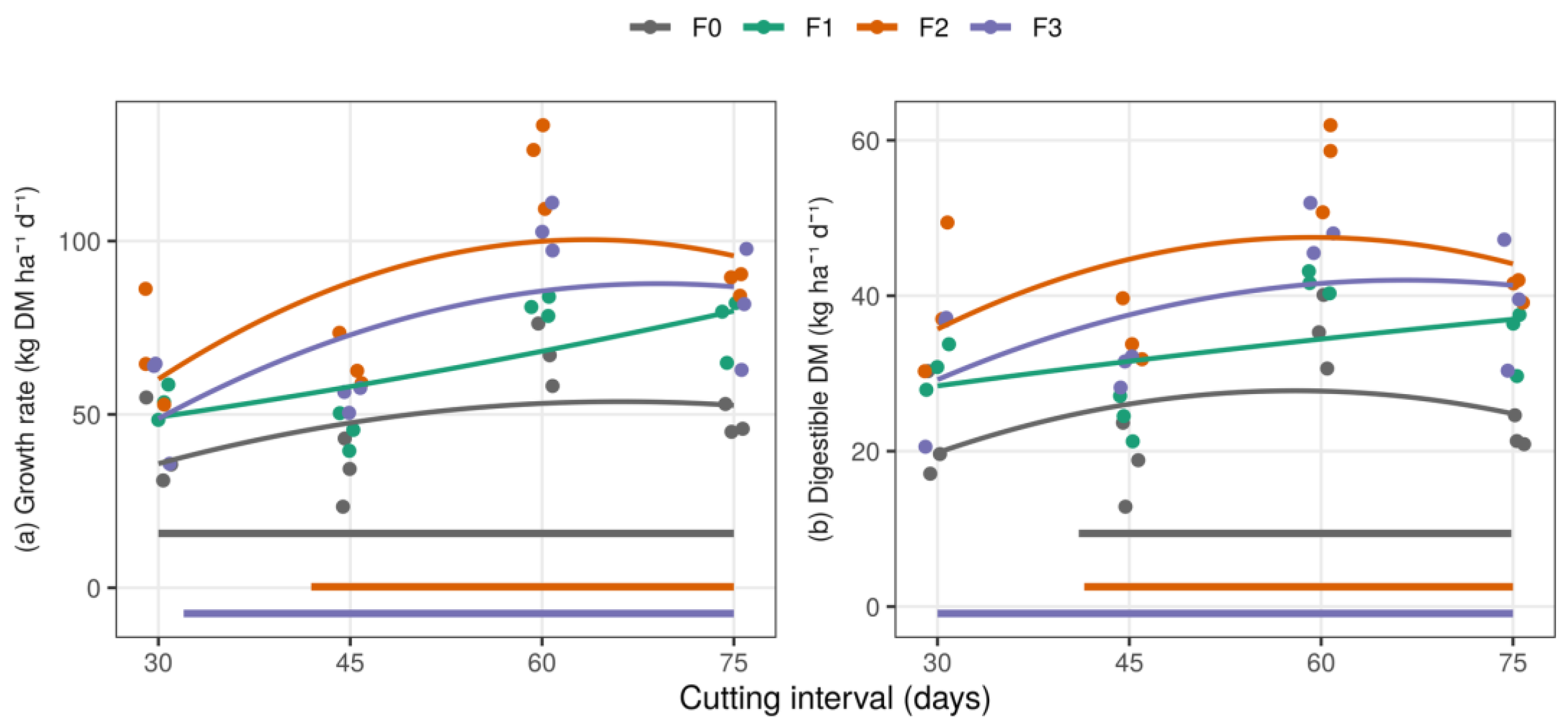
Figure 2.
Ratio of third- to first-cut yield (95% CI) by cycle and cutting interval. The dashed line indicates no change.
Figure 2.
Ratio of third- to first-cut yield (95% CI) by cycle and cutting interval. The dashed line indicates no change.
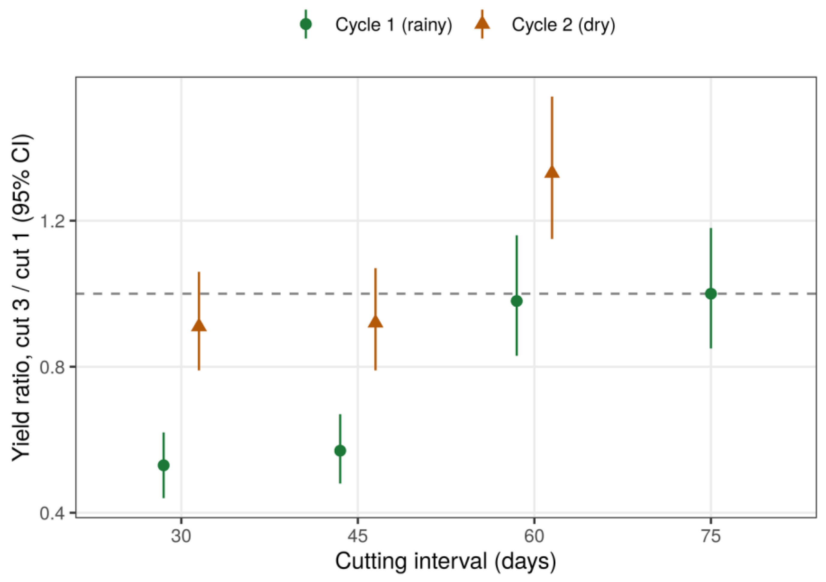
Figure 3.
Daily milk yield per cow in both periods. Dashed lines: mean of each period.
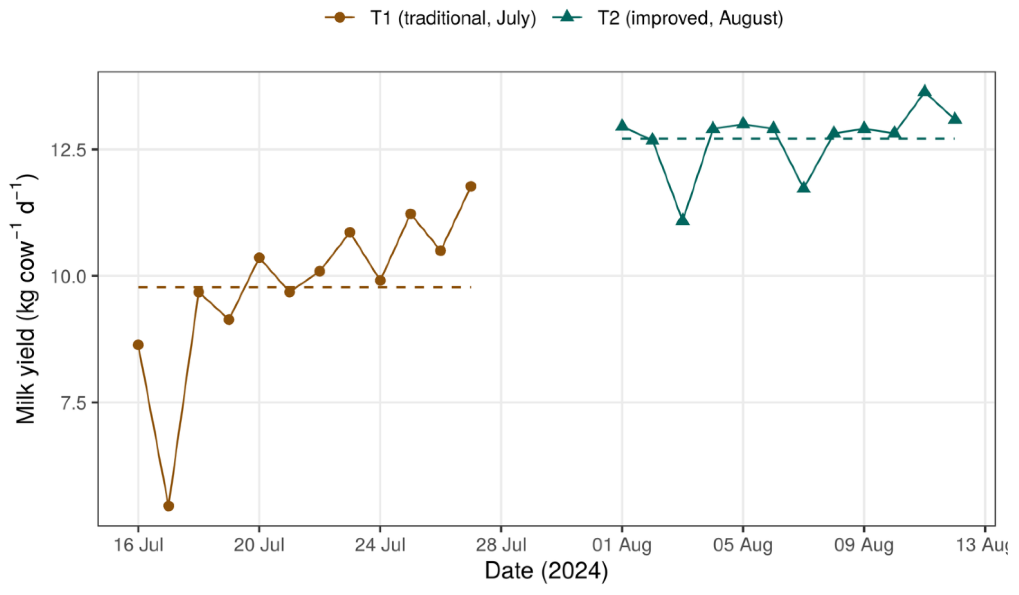
Table 1.
Nutrient supply per treatment (kg ha−1, sum of the two applications).
| Treatment | N | P2O5 | K2O | CaO | MgO | S | Zn | Cu | Mn | B |
| F0 | 0 | 0 | 0 | 0 | 0 | 0 | 0 | 0 | 0 | 0 |
| F1 | 64 | 63.3 | 118 | 230.4 | 190 | 155.5 | 0.253 | 0.15 | 0.20 | 0.624 |
| F2 | 110 | 86.3 | 202 | 264.4 | 234 | 222.9 | 0.253 | 0.15 | 0.20 | 0.624 |
| F3 | 156 | 109.3 | 286 | 298.4 | 278 | 298.6 | 0.253 | 0.15 | 0.20 | 0.624 |
F0: no fertilisation; F1: low fertilisation; F2: according to soil requirement; F3: high fertilisation.
Table 3.
Dry matter yield per cut (DM), plant height and growth rate (GR) by fertilisation level and cutting interval in each evaluation cycle.
Table 3.
Dry matter yield per cut (DM), plant height and growth rate (GR) by fertilisation level and cutting interval in each evaluation cycle.
| Cycle 1 (rainy) | Cycle 2 (dry) | |||||
| Level | DM (kg ha−1) | Height (cm) | GR (kg ha−1 d−1) | DM (kg ha−1) | Height (cm) | GR (kg ha−1 d−1) |
| Fertilisation | ||||||
| F0 | 2216 c | 26.8 c | 44.6 c | 1149 c | 29.5 c | 26.6 c |
| F1 | 3066 b | 36.8 b | 61.8 b | 1640 b | 30.1 bc | 37.9 b |
| F2 | 4120 a | 46.0 a | 83.0 a | 2024 ab | 33.2 ab | 46.8 ab |
| F3 | 3489 ab | 44.0 a | 70.3 ab | 2096 a | 35.0 a | 48.4 a |
| Cutting interval | ||||||
| 30 d | 1519 c | 24.4 c | 50.6 c | 1297 b | 23.4 c | 43.2 a |
| 45 d | 2122 b | 27.6 c | 47.2 c | 1354 b | 27.6 b | 30.1 b |
| 60 d | 5600 a | 46.7 b | 93.3 a | 2707 a | 44.8 a | 45.1 a |
| 75 d | 5411 a | 54.8 a | 72.1 b | – | – | – |
DM and GR: mean back-transformed from the log scale with bias correction. Within each factor and column, different letters indicate differences by Tukey’s test (p < 0.05), using each factor’s error stratum. Ratios between levels with 95% CI are given in the Supplementary Materials.
Table 4.
Cumulative production over three successive cuts expressed as annual equivalent (kg DM ha−1 yr−1).
Table 4.
Cumulative production over three successive cuts expressed as annual equivalent (kg DM ha−1 yr−1).
| Cycle | Interval | F0 | F1 | F2 | F3 |
| 1 | 30 d | 14,772 | 19,536 | 24,773 | 20,002 |
| 1 | 45 d | 12,256 | 16,476 | 23,741 | 20,025 |
| 1 | 60 d | 24,516 | 29,606 | 44,890 | 37,840 |
| 1 | 75 d | 17,504 | 27,575 | 32,146 | 29,493 |
| 2 | 30 d | 10,866 | 15,919 | 18,118 | 19,211 |
| 2 | 45 d | 7280 | 10,166 | 14,906 | 13,351 |
| 2 | 60 d | 12,030 | 15,749 | 17,984 | 21,972 |
Annual equivalent = cumulative production/(3 × interval) × 365. Mean of three blocks.
Table 5.
Ratio of third- to first-cut yield (cut 3/cut 1) by cutting interval and cycle.
| Cycle | Interval | Ratio | 95% CI | t | p |
| 1 | 30 d | 0.53 | 0.44–0.62 | −7.61 | <0.001 |
| 1 | 45 d | 0.57 | 0.48–0.67 | −6.67 | <0.001 |
| 1 | 60 d | 0.98 | 0.83–1.16 | −0.28 | 0.784 |
| 1 | 75 d | 1.00 | 0.85–1.18 | 0.00 | 0.996 |
| 2 | 30 d | 0.91 | 0.79–1.06 | −1.25 | 0.219 |
| 2 | 45 d | 0.92 | 0.79–1.07 | −1.14 | 0.259 |
| 2 | 60 d | 1.33 | 1.15–1.54 | 3.91 | <0.001 |
Estimated from the log-scale contrast of the mixed model of each cycle (df = 64 in cycle 1 and 48 in cycle 2).
Table 6.
Botanical composition (%) in cycle 1 estimated from the isometric log-ratio balances (ryegrass, white clover and weeds).
Table 6.
Botanical composition (%) in cycle 1 estimated from the isometric log-ratio balances (ryegrass, white clover and weeds).
| Factor | Level | Ryegrass | White clover | Weeds |
| Fertilisation | F0 | 55.8 | 9.2 | 35.0 |
| F1 | 67.6 | 12.8 | 19.6 | |
| F2 | 78.3 | 6.8 | 15.0 | |
| F3 | 75.4 | 8.8 | 15.8 | |
| Interval | 30 d | 68.8 | 7.5 | 23.8 |
| 45 d | 63.7 | 14.7 | 21.6 | |
| 60 d | 65.8 | 9.9 | 24.4 | |
| 75 d | 79.9 | 6.7 | 13.4 | |
| Cut | 1 | 68.4 | 13.8 | 17.8 |
| 2 | 72.4 | 9.1 | 18.4 | |
| 3 | 68.1 | 6.3 | 25.6 |
Means back-transformed from the balances (geometric means close to 100), which therefore differ from arithmetic means of percentages. Zeros replaced multiplicatively; D. glomerata analysed separately. p-values, ryegrass/clover balance: fertilisation 0.247, interval < 0.001, cut < 0.001, interval × cut < 0.001; sown/weeds balance: fertilisation 0.132, interval 0.172, cut 0.009, interval × cut 0.016.
Table 7.
Change in nutritive value per additional day of regrowth, cycle 1 (analysis of covariance, n = 16 composite samples).
Table 7.
Change in nutritive value per additional day of regrowth, cycle 1 (analysis of covariance, n = 16 composite samples).
| Variable | Mean at 30 d (%) | Mean at 75 d (%) | Slope (points d−1) | 95% CI | p | Adjusted p |
| CP | 17.25 | 12.24 | −0.109 | −0.147 to −0.072 | <0.001 | <0.001 |
| NDF | 53.70 | 63.41 | 0.227 | 0.163 to 0.292 | <0.001 | <0.001 |
| ADF | 39.09 | 42.34 | 0.102 | −0.039 to 0.242 | 0.139 | 0.139 |
| IVDMD | 56.90 | 46.73 | −0.239 | −0.304 to −0.174 | <0.001 | <0.001 |
| Ash | 10.04 | 6.32 | −0.079 | −0.107 to −0.051 | <0.001 | <0.001 |
Model with regrowth days (covariate) and fertilisation (factor); residual df = 11. p-values adjusted by the false discovery rate across the five variables. CP: crude protein; NDF: neutral detergent fibre; ADF: acid detergent fibre; IVDMD: in vitro dry matter digestibility.
Table 8.
Supply, removal accumulated over the two cycles and balance (supply − removal) of N and K2O (kg ha−1).
Table 8.
Supply, removal accumulated over the two cycles and balance (supply − removal) of N and K2O (kg ha−1).
| Interval | Nutrient | Trt. | Supply | Removal | Balance | 95% CI |
| 30 d | N | F0 | 0 | 178 | −178 | −280 to −75 |
| F1 | 64 | 258 | −194 | −271 to −117 | ||
| F2 | 110 | 277 | −167 | −367 to 32 | ||
| F3 | 156 | 285 | −129 | −280 to 21 | ||
| K2O | F0 | 0 | 162 | −162 | −341 to 17 | |
| F1 | 118 | 258 | −140 | −345 to 64 | ||
| F2 | 202 | 370 | −168 | −369 to 32 | ||
| F3 | 286 | 326 | −40 | −51 to −29 | ||
| 60 d | N | F0 | 0 | 540 | −540 | −910 to −171 |
| F1 | 64 | 706 | −642 | −1871 to 588 | ||
| F2 | 110 | 1114 | −1004 | −1347 to −660 | ||
| F3 | 156 | 672 | −516 | −1068 to 37 | ||
| K2O | F0 | 0 | 646 | −646 | −865 to −427 | |
| F1 | 118 | 712 | −594 | −787 to −400 | ||
| F2 | 202 | 1093 | −891 | −1415 to −368 | ||
| F3 | 286 | 1094 | −808 | −1404 to −211 |
Supply according to Table 1, taken as the total for the experiment. Removal = dry-basis concentration × cumulative DM of three cuts per cycle, summed over both cycles. CI based on t with three blocks (df = 2).
Table 10.
Intake, milk yield and composition, energy-corrected milk (ECM) and feed efficiency (FE) by period.
Table 10.
Intake, milk yield and composition, energy-corrected milk (ECM) and feed efficiency (FE) by period.
| Variable | n | T1 | T2 | Difference (95% CI) | p | Adjusted p | Hedges’ g (95% CI) |
| DM intake (kg cow−1 d−1) | 3 | 9.97 | 13.24 | 3.27 (1.41 to 5.13) | 0.009 | – | 3.31 (0.85 to 5.77) |
| Milk (kg cow−1 d−1) a | 12 | 9.78 | 12.71 | 2.92 (1.35 to 4.50) | <0.001 | – | – |
| MUN (mg dL−1) | 3 | 12.55 | 13.30 | 0.75 (−0.38 to 1.87) | 0.112 | 0.448 | 1.63 (−0.22 to 3.47) |
| Fat (%) | 3 | 3.96 | 4.16 | 0.20 (−1.08 to 1.49) | 0.579 | 0.579 | 0.43 (−1.19 to 2.04) |
| Protein (%) | 3 | 3.25 | 3.45 | 0.20 (−0.26 to 0.66) | 0.294 | 0.579 | 0.79 (−0.87 to 2.45) |
| Total solids (%) | 3 | 12.79 | 13.15 | 0.36 (−1.04 to 1.76) | 0.468 | 0.579 | 0.54 (−1.09 to 2.17) |
| ECM (kg cow−1 d−1) b | – | 9.69 | 13.12 | 3.43 (2.28 to 4.75) | – | – | – |
| FE (kg ECM kg−1 DM) b | – | 0.97 | 0.99 | 0.02 (−0.13 to 0.16) | – | – | – |
Welch’s t test unless indicated. a Generalised least squares with AR(1) between days; herd yield divided by 11 cows. b Calculated from period means; CI by bootstrap stratified by source; no hypothesis test. Adjustment by false discovery rate within the milk composition family. MUN: milk urea nitrogen.
Table 11.
Nutritive value of the pasture on offer in each period (n = 3).
| Variable | T1 | T2 | Difference (95% CI) | p | Adjusted p |
| Ash (% DM) | 6.66 | 8.23 | 1.57 (0.36 to 2.78) | 0.023 | 0.068 |
| CP (% DM) | 11.83 | 14.48 | 2.65 (1.21 to 4.09) | 0.007 | 0.042 |
| NDF (% DM) | 49.46 | 49.08 | −0.39 (−16.46 to 15.68) | 0.933 | 0.933 |
| ADF (% DM) | 27.66 | 29.27 | 1.61 (−5.94 to 9.15) | 0.573 | 0.933 |
| IVDMD (%) | 59.78 | 60.57 | 0.79 (−7.00 to 8.58) | 0.779 | 0.933 |
| ME (Mcal kg−1 DM) | 2.05 | 2.08 | 0.03 (−0.27 to 0.33) | 0.779 | 0.933 |
Welch’s t-test; adjustment by false discovery rate across the six variables. ME: metabolisable energy.
Table 12.
Haematological and biochemical values of lactating cows by period (n = 5 per period).
| Variable | T1 | T2 | Difference (95% CI) | p | Adjusted p |
| Haematology | |||||
| RBC (×106 µL−1) | 5.87 | 7.73 | 1.86 (0.37 to 3.35) | 0.026 | 0.077 |
| Hb (g dL−1) a | 9.46 | 12.88 | 3.42 (1.15 to 5.68) | 0.014 | 0.055 |
| Hct (%) | 28.68 | 38.34 | 9.66 (6.14 to 13.18) | 0.001 | 0.017 |
| MCV (fL) b | 48.86 | 50.13 | 1.27 (−4.45 to 6.99) | 0.583 | 0.700 |
| MCH (pg) a | 16.12 | 16.73 | 0.61 (−0.96 to 2.18) | 0.358 | 0.478 |
| MCHC (g dL−1) a | 33.00 | 33.49 | 0.49 (−2.74 to 3.73) | 0.694 | 0.757 |
| Leukocytes (×103 µL−1) | 12.85 | 12.53 | −0.32 (−2.99 to 2.35) | 0.788 | 0.788 |
| Segmented neutrophils (%) | 36.8 | 47.8 | 11.0 (−2.7 to 24.7) | 0.095 | 0.191 |
| Lymphocytes (%) | 51.2 | 42.6 | −8.6 (−23.3 to 6.1) | 0.195 | 0.334 |
| Monocytes (%) | 4.6 | 6.8 | 2.2 (−0.2 to 4.6) | 0.067 | 0.160 |
| Eosinophils (%) | 7.4 | 2.8 | −4.6 (−7.0 to −2.2) | 0.003 | 0.020 |
| Platelets (×103 µL−1) | 260.2 | 305.8 | 45.6 (−48.1 to 139.3) | 0.288 | 0.432 |
| Serum biochemistry | |||||
| Urea (mg dL−1) | 26.40 | 28.42 | 2.02 (−4.82 to 8.86) | 0.498 | 0.732 |
| Creatinine (mg dL−1) | 0.65 | 0.74 | 0.09 (−0.03 to 0.22) | 0.113 | 0.275 |
| Total bilirubin (mg dL−1) | 0.34 | 0.33 | −0.01 (−0.06 to 0.04) | 0.648 | 0.768 |
| Direct bilirubin (mg dL−1) | 0.13 | 0.11 | −0.02 (−0.07 to 0.04) | 0.436 | 0.732 |
| Indirect bilirubin (mg dL−1) | 0.21 | 0.22 | 0.01 (−0.07 to 0.09) | 0.809 | 0.857 |
| Total protein (g dL−1) | 6.34 | 7.30 | 0.96 (0.28 to 1.63) | 0.013 | 0.110 |
| Albumin (g dL−1) | 2.99 | 3.25 | 0.26 (0.04 to 0.48) | 0.032 | 0.130 |
| Globulin (g dL−1) | 3.35 | 4.05 | 0.70 (0.05 to 1.34) | 0.038 | 0.130 |
| GGT (U L−1) | 23.42 | 26.72 | 3.30 (−1.34 to 7.94) | 0.137 | 0.292 |
| AST (U L−1) | 89.4 | 79.4 | −10.0 (−18.0 to −2.0) | 0.022 | 0.127 |
| ALT (U L−1) | 27.0 | 26.6 | −0.4 (−2.5 to 1.7) | 0.678 | 0.768 |
| Alkaline phosphatase (U L−1) | 105.8 | 101.4 | −4.4 (−19.6 to 10.8) | 0.516 | 0.732 |
| Calcium (mg dL−1) | 9.18 | 10.02 | 0.84 (0.01 to 1.67) | 0.049 | 0.139 |
| Phosphorus (mg dL−1) | 7.04 | 6.27 | −0.77 (−2.15 to 0.61) | 0.205 | 0.387 |
| Magnesium (mg dL−1) | 3.79 | 3.16 | −0.63 (−0.99 to −0.27) | 0.004 | 0.064 |
| Potassium (mEq L−1) | 3.75 | 3.78 | 0.03 (−0.43 to 0.50) | 0.857 | 0.857 |
| BHB (mmol L−1) | 1.10 | 1.04 | −0.06 (−0.34 to 0.22) | 0.633 | 0.768 |
Welch’s t test, independent samples. Adjustment by false discovery rate within haematology (12 variables) and serum biochemistry (17 variables). a Hb in T1 estimated as 0.33 × Hct; comparison not valid. b MCV recalculated as Hct/RBC × 10.
Disclaimer/Publisher’s Note: The statements, opinions and data contained in all publications are solely those of the individual author(s) and contributor(s) and not of MDPI and/or the editor(s). MDPI and/or the editor(s) disclaim responsibility for any injury to people or property resulting from any ideas, methods, instructions or products referred to in the content. |
© 2026 by the authors. Licensee MDPI, Basel, Switzerland. This article is an open access article distributed under the terms and conditions of the Creative Commons Attribution (CC BY) license (http://creativecommons.org/licenses/by/4.0/).
Copyright: This open access article is published under a Creative Commons CC BY 4.0 license, which permit the free download, distribution, and reuse, provided that the author and preprint are cited in any reuse.