

Submitted:
09 November 2026
Posted:
11 November 2026
You are already at the latest version
Abstract
Finite-shot quantum tomography often leaves a posterior over many density matrices compatible with the same measurement record, but fast reconstruction methods collapse this uncertainty to a single state. We frame this setting as amortized posterior sampling and introduce BuresTomFlow, a measurement-conditioned Flow Matching sampler for full-rank density matrices. The method transports base density matrices along Bures-Wasserstein paths on the positive matrix cone, projects the path back to the trace-one state space, and trains the velocity field with a Bures-aligned tangent loss. Thus the sampler is trained in the same fidelity-based geometry used to judge posterior quality. We evaluate BuresTomFlow in dense four-qubit simulations with count, shadow, and mixed measurement records. Against Cholesky, log-density, and generic Riemannian Flow Matching controls at comparable learned-sampler runtime, BuresTomFlow improves Bures distance, credible-ball coverage, and held-out observable prediction. In the main comparison across multiple seeds, mean Bures distance decreases from 0.618 for the Cholesky baseline to 0.367 for BuresTomFlow, and mean coverage error decreases from 0.203 to 0.100. These results show that the value of Bures geometry is not merely enforcing physical states, but producing calibrated posterior uncertainty when finite-record tomography cannot be reduced to one reconstruction.
Keywords:
flow matching
; posterior
; quantum tomography
1. Introduction
Quantum state tomography infers an unknown density matrix from measurement data. In many finite-record regimes, however, the data do not determine a single plausible state. Low-shot Pauli counts, classical-shadow records, and mixed measurements can leave a posterior family of density matrices that agree with the observations while disagreeing on fidelity, held-out observables, or repeated-run calibration. Collapsing this family to one reconstruction removes the uncertainty that the experiment actually leaves.
This posterior objective is inherently geometric. The unknown state is constrained to the positive semidefinite, trace-one state space, and quantum states are naturally compared by fidelity and Bures-type distances rather than entrywise Euclidean error. A tomography posterior sampler must therefore satisfy three requirements at once: produce physical density matrices, represent multiple plausible states conditioned on the same record, and calibrate uncertainty in a geometry matched to quantum-state distinguishability.
Existing tomography pipelines meet these requirements only partially. Linear inversion and maximum-likelihood estimators provide efficient point estimates, but they require projection or regularization under sparse records and do not represent posterior uncertainty. Bayesian and Markov-chain methods expose uncertainty, but they can be expensive for each new measurement record. Neural tomography amortizes reconstruction, yet most learned approaches optimize reconstruction or observable prediction rather than a density-matrix posterior whose paths, losses, and calibration checks are geometry aligned.
We introduce BuresTomFlow, a measurement-conditioned Flow Matching sampler for full-rank density matrices. Starting from base density matrices, the model learns velocity fields along Bures-Wasserstein positive-matrix paths, projects intermediate states back to the trace-one state space, and trains with Bures-aligned tangent supervision. This construction makes the metric a modeling ingredient rather than a post-processing score: the same fidelity-based geometry shapes the training paths and evaluates posterior samples.
Empirically, this geometry is not interchangeable with generic physical parameterizations. Across multi-seed dense four-qubit experiments, BuresTomFlow improves Bures distance, posterior coverage, and held-out observable prediction over Cholesky, log-density, and vanilla Riemannian Flow Matching controls at comparable learned-sampler runtime. The gains are clearest in low-shot shadow, count, and mixed measurement regimes, where the data leave meaningful posterior ambiguity.
Figure 1 summarizes the pipeline: finite measurement records condition the velocity field, Bures-Wasserstein paths define the training target, and posterior samples are evaluated by state-space error, calibration, observable prediction, and runtime.
Contributions. The main contributions are:
- We formulate finite-record quantum tomography as amortized posterior sampling over density matrices, evaluated by Bures distance, credible-region coverage, held-out observable error, and learned-sampler runtime.
- We develop a Bures-geometric conditional Flow Matching construction for density matrices, including Bures-Wasserstein paths, tangent supervision, and trace-one projection.
- We isolate the role of geometry through Cholesky, log-density, generic Riemannian, and point-estimation controls, and organize the results by measurement regime.
2. Related Work and Background
2.1. Finite-Record Quantum Tomography
Tomography under finite records. Quantum state tomography estimates a density matrix from measurement data, with classical estimators, Bayesian methods, compressed-sensing variants, and randomized-measurement protocols covering different regimes [1,5,14,16,17,18,25]. A point estimate can be sufficient when the record is highly informative. In the finite Pauli and shadow settings studied here, however, the record leaves posterior ambiguity over compatible physical states. We therefore use the record as a conditioning variable for posterior sampling rather than as input to one estimator. Appendix A gives the fuller tomography background.
Neural tomography. Neural tomography and conditional generative tomography learn fast reconstruction or generation maps from measurement statistics [2,8,9,27,29,31,35]. The distinction here is the target: calibrated posterior samples over density matrices, evaluated by Bures distance, held-out observables, and credible-region coverage.
2.2. Flow Matching and Posterior Sampling
Flow matching and posterior inference. Amortized neural posterior estimation learns conditional distributions from simulated parameter–observation pairs rather than running separate inference for each observation [13]. Flow Matching and closely related rectified-flow and stochastic-interpolant formulations train continuous-time generative models by regressing velocity fields along prescribed probability paths [3,21,23]. In standard notation, a base sample is coupled with a target sample , and the path and regression loss are
Conditional Flow Matching (CFM) adds a condition c to the same regression, replacing by and using endpoint pairs drawn under the condition. Minibatch optimal transport variants make the choice of coupling part of the model [30]. Riemannian Flow Matching extends the same regression principle to non-Euclidean domains [10], and Flow Matching posterior estimation applies it to simulation-based inference [34]. These tools specify how to train conditional flows. The modeling question here is which geometry should define paths, velocities, and losses for posterior density-matrix tomography. We use credible-region coverage as a posterior-calibration metric, related to but not replacing full simulation-based calibration with rank statistics [28].
For the posterior-tomography instance, the condition is the measurement record y. A base state is coupled with a posterior target , a path is chosen, and the network is trained to match the corresponding velocity:
The path , velocity , and norm in Eq. (2) are where geometric assumptions enter the model.
2.3. Geometric Flow Matching
Riemannian Flow Matching. Riemannian Flow Matching replaces Euclidean straight-line paths with geometry-aware paths on a manifold [10]. For points on a Riemannian manifold , the geodesic path and its velocity are
The corresponding velocity-regression loss is
Thus the geometry enters through the path, tangent velocity, and norm. BuresTomFlow follows this principle, but the geometry is chosen from the posterior-tomography target itself: Bures-Wasserstein positive-matrix transport rather than a generic chart.
Geometry-aware flow models. Recent geometric flow models follow this problem-driven pattern by adapting flow-based generation to structured output spaces such as SPD matrices and SE(3) poses [12,24]. In posterior tomography, the structured object is a density matrix, the condition is a finite quantum measurement record, and the central evaluation target is calibrated uncertainty under quantum-state metrics. The contribution is therefore not another generic manifold flow, but a posterior-tomography construction whose value is judged by posterior quality.
2.4. Bures Geometry for Density Matrices
Bures geometry and quantum optimal transport. Fidelity and Bures distance compare quantum states through distinguishability rather than entrywise matrix error [7,19,32]. Bures-Wasserstein geometry gives closed-form positive-matrix transport operations [4]. Because trace-one density matrices are not a geodesic submanifold of the positive cone [33], BuresTomFlow uses positive-cone interpolation followed by projection back to the physical state space. This choice is not only a positivity constraint. Cholesky, log-density, and generic Riemannian parameterizations can preserve physical-looking matrices, while the tested claim is that posterior sampling improves when the training geometry is aligned with the fidelity-based geometry used for evaluation.
Positioning. The gap is therefore a posterior-sampling problem, not merely a reconstruction problem. Tomography, amortized posterior inference, Flow Matching, and Bures geometry exist separately, but they have not been combined into a density-matrix posterior sampler whose paths, training loss, and uncertainty checks are aligned with the metric used to judge quantum states. The main experiments isolate this adaptation by comparing BuresTomFlow against Cholesky, log-density, vanilla Riemannian Flow Matching, and point-estimation controls.
3. BuresTomFlow
3.1. Posterior Tomography Target
Finite-record tomography is a conditional generation problem on the density-matrix state space, rather than a deterministic regression problem. For an n-qubit system with , the physical domain is
A measurement record is generated from Born probabilities, and the corresponding Bayesian tomography posterior is [25]
The role of BuresTomFlow is to amortize this conditional distribution: for a new finite record y, the sampler returns
where is trained to approximate the posterior family induced by the simulator and measurement model.
The training pairs come from the joint law rather than from hand-labeled posterior clouds. We draw a latent state , simulate a finite record , and use the pair for conditional Flow Matching. Under this prior-predictive sampling scheme, the conditional law of given y is exactly the posterior in Eq. (6). The neural sampler therefore learns posterior samples by seeing many simulated inverse problems. This is the same reason the method targets a sample cloud rather than a single reconstruction: when y is sparse, several states remain plausible under the same record.
3.2. Measurement-Conditioned Velocity Field
The measurement record is treated as an unordered set of tokens. Each token encodes the product-Pauli setting, the measured bit pattern or aggregate count summary, the shot budget, and the token type:
Here denotes the local measurement basis, stores bit-level outcomes for shadow snapshots or averaged bits for count records, stores an all-plus/count statistic, is the shot count, and distinguishes snapshot and count tokens. Shadow records use randomized Pauli settings. Count records aggregate repeated shots for fixed settings. Mixed records concatenate the two. The map is implemented as either a Deep Sets encoder or a small masked self-attention encoder.
The velocity network receives the current matrix, time, and record context. In the dense four-qubit model, the input feature vector is the real-imaginary matrix representation augmented by time and the record embedding:
Before the velocity is used in either a Bures or Frobenius loss, a matrix proposal is projected onto the Hermitian trace-free tangent space:
Thus the network learns trace-preserving density-matrix directions rather than arbitrary complex matrices.
3.3. Bures-Wasserstein Probability Paths
The geometric choice enters before any evaluation metric is computed. BuresTomFlow builds probability paths using Bures-Wasserstein transport on the positive matrix cone, then returns each intermediate point to the trace-one state space. Full-rank states are used in the main dense experiments because the matrix square roots and inverse square roots in the Bures map become singular at the boundary.
When a density-matrix target may be close to the boundary, it is first moved into the interior by the depolarizing mixture . This smoothing is separate from the projection used for a general matrix proposal. If , define for a small floor . The density-matrix projection is
Given a base state and a smoothed target , the positive-cone Bures-Wasserstein transport map defines the positive factor [4]:
The interpolation uses the affine factor , transports the base state in the positive cone as , and then returns the path to the trace-one domain:
All derivatives are computed through the differentiable matrix operations defining Eqs. (12) and (13). The important modeling point is that is not an ambient straight line between two matrices. The path first follows the positive-matrix geometry associated with fidelity and only then applies the trace-one constraint required by tomography.
This projection is part of the learned probability path rather than a post-hoc validity repair. The sampler is trained on the differentiated projected path, the velocity loss is evaluated after tangent projection, and posterior quality is measured with the same Bures distance. Thus the method couples three objects that are often separated in reconstruction pipelines: the physical density-matrix domain, the velocity geometry, and the uncertainty metric. Appendix B gives the positive-cone interpolation, projection, and tangent-metric details.
3.4. Bures-Aligned Training Objective
The conditional velocity field is trained by matching the Bures path velocity in the local Bures tangent metric. For a Hermitian trace-free tangent direction , the metric is defined through the Lyapunov operator :
The resulting tangent norm is
Write the projected velocity residual as . With the Bures tangent norm, the Flow Matching objective becomes
following the Flow Matching and Riemannian Flow Matching regression principle [10,21]. The Lyapunov equation defines the local Bures tangent norm, so the loss penalizes velocity errors according to the same local geometry used by the Bures distance. A Frobenius loss can still preserve Hermitian trace-free outputs after projection, but it does not weight tangent directions by the local density-matrix geometry.
For finite-record training, we use a tomography-specific variant that keeps the same Bures velocity term and adds a low-shot endpoint consistency penalty. The predicted endpoint obtained by following the velocity for the remaining time is
The sparse-record weight increases the contribution of low-shot records while remaining bounded. The finite-record loss is
The endpoint term asks whether the predicted velocity, if followed for the remaining time, points toward the latent state that generated the record. The shot-dependent weight makes sparse records contribute more strongly without letting any one regime dominate training.
3.5. Training and Posterior Sampling
The training construction can be written compactly as
The optimizer updates so that matches under Eq. (16) or Eq. (18). This makes the learned object a measurement-conditioned vector field on density matrices, not a decoder that emits one matrix from one record.
At test time the record is fixed and uncertainty comes from independent base states. For , draw and integrate
In the dense implementation, the same record context is reused across all S trajectories, while the base density matrix is resampled for each posterior draw. The ODE integration applies the density-matrix projection used in Eq. (11) at intermediate and terminal states, so the posterior cloud remains a collection of physical states throughout sampling. Posterior spread is produced by the learned conditional transport, not by rerunning a separate reconstruction algorithm for each sample. The sample set is then a posterior object whose mean gives a reconstruction, whose spread gives credible balls, and whose pushforward through observables gives predictive uncertainty.
4. Experiments
The experiments test whether Bures-aligned Flow Matching improves posterior samples under finite records. We compare against Cholesky, vanilla Riemannian Flow Matching, log-density chart controls, and linear inversion across count, shadow, and mixed measurement records. The metrics are Bures distance, coverage error, held-out observable error, and amortized runtime.
4.1. Experimental Setup
We evaluate synthetic posterior tomography tasks over full-rank 4-qubit density matrices. The measurement regimes include count, classical-shadow, and mixed records, with shot budgets ranging from low-shot to more informative settings. These regimes stress posterior uncertainty: an underdetermined record requires a distribution over compatible states, not only a plausible single estimate.
Targets are full-rank four-qubit thermal states from an open-boundary transverse-field Ising Hamiltonian [26],
We sample , , and , then add a small identity floor to keep targets full rank.
Measurement records are sampled from product-Pauli Born probabilities. Shadow records draw a fresh product-Pauli basis for each shot, count records aggregate repeated shots over a fixed prefix of 32 product-Pauli settings, and mixed records concatenate both views for the same latent state. Regime names such as shadow-16 and mixed-32 denote the measurement family and shot budget.
Implementation summary. All dense posterior experiments use density matrices. The sampler uses a Set Transformer record encoder [20], a time-conditioned velocity network, Adam with learning rate , batch size 8, 420 optimization steps per comparison, 32 posterior samples per record, and Euler integration with step size 0.25. Appendix C gives the full implementation details.
4.2. Baselines and Metrics
The baseline set separates physical parameterization, generic manifold machinery, convenient positive-matrix charts, and point estimation. Cholesky parameterization tests whether positivity-preserving coordinates are enough. Vanilla Riemannian Flow Matching uses manifold machinery without the Bures-specific path and tangent construction. Log-Euclidean and mirror/Frobenius variants form a log-density chart family. Linear inversion acts as a fast point-estimation control that does not produce calibrated posterior samples.
Metrics. We report Bures distance, held-out observable error, posterior coverage error, and runtime. These metrics test state accuracy, downstream prediction, uncertainty calibration, and sampling cost. Appendix D gives the full evaluation protocol, including rank calibration and physical-state diagnostics.
State-space accuracy. Bures distance is the primary geometry-aligned state metric. We use the trace-normalized positive-matrix form
which reduces to for trace-one density matrices [4,7]. For posterior samplers, we compare the true state with the projected posterior center
For point-estimation controls, the returned estimate plays the same role as this posterior center.
Held-out observables. Observable error asks whether posterior samples support accurate predictions on observables that are not directly used as the headline state-space distance:
Posterior calibration. Coverage error uses a credible-ball check. Given a nominal level , let be the empirical -quantile of . Across repeated synthetic tomography tasks , empirical coverage is
A low distance error alone is not sufficient for posterior tomography. The sample cloud must also match empirical coverage. Linear inversion is therefore marked as a point-estimation control.
Runtime. Runtime measures the practical cost of amortized posterior sampling. We compare learned samplers at inference time after training, so the relevant question is whether the Bures-geometric quality gains are obtained at runtime comparable to the learned geometry baselines.
Regime-level evidence. Averaging across measurement settings would hide the finite-record structure of the task. We therefore separate count, mixed, and randomized shadow records and ask whether the Bures-specific construction remains advantageous when observations are sparse or heterogeneous. These are the settings in which posterior ambiguity is most visible, and they are the settings that best test calibrated posterior sampling.
4.3. Main Posterior Tomography Results
Table 1 gives the compact multi-seed geometry comparison. BuresTomFlow has the best posterior-sampler quality metrics while running at comparable learned-sampler cost.
The baseline pattern isolates the source of the improvement. Cholesky already encodes positive definiteness, so the advantage is not simply physical validity. Vanilla Riemannian Flow Matching uses manifold machinery without the Bures-specific path and tangent construction, so the advantage is not simply the use of a Riemannian solver. Log-density chart controls show that convenient positive-matrix coordinates can still be poorly calibrated as posterior samplers.
Point-estimation control. Linear inversion is the fast-reconstruction baseline. Its role clarifies the contribution: the posterior formulation targets calibrated uncertainty over physical density matrices, not only a single-state estimate.
4.4. Finite-Record Measurement Regimes
Figure 2 reports the comparison by measurement regime. The seed-level panels show that the ordering is not an artifact of averaging across count, mixed, and shadow records.
4.5. Control Experiments
Table 1 also functions as the component comparison: the controls remove Bures transport, Bures tangent supervision, or posterior sampling. Their ordering ties the improvement to the Bures-specific path and tangent construction rather than physical validity alone. The full control table is deferred to Appendix E.
A Bures-localized rank check gives the same ordering as the main calibration comparison. The full rank-calibration values are reported in Appendix G.
5. Conclusions, Limitations, and Future Work
We introduced BuresTomFlow, a Bures-geometric conditional Flow Matching sampler for finite-record posterior quantum tomography. The method treats tomography as calibrated sampling over physical density matrices rather than as single-state reconstruction, and the experiments isolate the gains from the Bures-specific path and tangent construction. The current dense implementation focuses on exact 4-qubit tomography. Rank-calibration and Bures-kernel scaling results support the same geometry-aligned story, while full larger-qubit posterior tomography remains future work.
Funding
NEED TO BE FILLED BEFORE FINAL SUBMISSION.
Conflicts of Interest
The authors declare that they have no conflict of interest.
Appendix A. Measurement Protocol and Estimators
Finite-record quantum tomography. Quantum state tomography is a statistical inverse problem on the convex set of density matrices. Standard approaches include linear inversion, maximum likelihood, and Bayesian estimation [5,17,25]. A point estimator can be accurate when the measurement record is highly informative, but finite records typically leave many physical states with comparable likelihood. Practical Bayesian tomography addresses this ambiguity by representing uncertainty over states rather than returning a single reconstruction [15]. BuresTomFlow follows this posterior viewpoint while amortizing inference: after training, the same conditional sampler can be queried for density-matrix posterior samples from a new finite record.
Randomized measurements and shadow records. The conditioning input is a finite measurement record rather than the true state. We use count, mixed, and randomized shadow records to represent increasingly heterogeneous observation settings. Shadow tomography and classical shadows use randomized measurements to predict many observables without reconstructing every matrix entry [1,18]. Broader randomized-measurement protocols are reviewed in Ref. [14]. In this paper, shadow records are not used as a substitute for posterior uncertainty. They are one family of finite records from which the sampler must infer a distribution over compatible density matrices.
Synthetic state family. The main dense benchmark uses full-rank four-qubit thermal states from an open-boundary transverse-field Ising Hamiltonian [26],
The implementation samples , , and , then mixes in a small identity component to keep the density matrix full rank. This construction gives a controlled target distribution with noncommuting terms, nontrivial eigenstructure, and exact access to the latent density matrix for evaluation. The full-rank floor is a numerical device for stable matrix square roots and logarithmic tangent calculations. It is not additional measurement information.
Record construction. All measurement records are encoded as fixed-width tokens carrying a product-Pauli basis label, outcome statistics, the shot budget, and a token type. Each four-qubit token has dimension 24: sixteen entries encode the per-qubit basis labels, four entries encode bit or mean-bit statistics, one entry stores the all-plus/count statistic, one entry stores the scaled shot budget, and two entries encode whether the token is a snapshot or count token. In shadow mode, each token is one randomized Pauli snapshot: a product-Pauli basis is sampled, a bitstring outcome is drawn from the Born probabilities of the latent state, and the token stores the measured basis and outcome summary. In count mode, the experiment uses aggregate count tokens over a fixed prefix of 32 product-Pauli settings. Each token stores mean bit statistics from repeated shots under the same basis. Mixed mode concatenates the shadow and count records for the same latent state. Thus the three measurement families differ in the information presented to the encoder, while the posterior target remains the same density matrix conditioned on the finite record.
Born sampling for product-Pauli records. For a product-Pauli setting and bitstring , let denote the tensor product of the one-qubit projectors onto the measurement eigenvectors specified by p and b. The record simulator samples outcomes from
Shadow records draw a fresh product-Pauli setting for each shot. Count records reuse a fixed prefix of the product-Pauli settings and store aggregate bit statistics for each setting. Mixed records concatenate both views. Consequently, all finite-record comparisons use the same Born rule and the same latent-state family, while varying only how the measurement information is packaged for the conditional encoder.
Relation to classical-shadow estimators. A randomized Pauli snapshot can also be converted into the classical-shadow estimator [18]. If maps the measured Pauli basis on qubit q to the computational basis and the observed bit is , the local inverse estimator is
This estimator explains why randomized Pauli snapshots are informative for observable prediction. BuresTomFlow uses the same physical measurement interface, but it does not average Eq. (27) into a single reconstructed state. The snapshot is kept as a conditioning token, and the learned model outputs posterior samples over density matrices compatible with the finite record.
Posterior estimators. For each measurement record y, the sampler returns a finite posterior cloud of positive trace-one matrices. Point summaries use the projected posterior center
where is the density-matrix projection defined in Appendix B. The full sample cloud is used for credible-ball coverage and rank-calibration checks. Linear inversion is evaluated as a reconstruction baseline but is not assigned posterior coverage metrics, because it produces a single matrix rather than a sample cloud.
Neural and amortized tomography. Neural quantum state tomography uses learned representations or generative models to reconstruct states from measurement statistics [8,31]. Conditional generative tomography is especially close in spirit, since it learns a measurement-conditioned generator whose output is mapped to a physical density matrix [2]. Later work explores convolutional and attention-based reconstruction [9,27], while diffusion-style quantum generative models target structure-preserving state generation or property estimation [29,35]. The present work differs in its evaluation target: it asks whether a learned sampler returns calibrated posterior samples over density matrices, not only whether it reconstructs one accurate state.
Appendix B. Bures Geometry and Projected Density-Matrix Flow
Bures geometry for density matrices. Fidelity and Bures distance compare quantum states through distinguishability rather than entrywise matrix error [7,19,32]. At the infinitesimal level, the Bures metric is proportional, up to convention, to the symmetric-logarithmic-derivative Fisher metric underlying the quantum Cramér–Rao bound [6]. On the positive-definite cone, Bures-Wasserstein geometry has closed-form transport maps, geodesics, means, and barycentres [4]. The trace-one density-matrix set is not a geodesic submanifold of this cone [33]. We therefore use positive-cone Bures-Wasserstein interpolation followed by projection back to the trace-one state space, rather than claiming that the trace-one path is itself an exact cone geodesic.
Distance used in the experiments. For positive matrices A and B, the Bures-Wasserstein distance used by the metrics is
For trace-one density matrices, is the paper’s , and . The implementation computes Eq. (29) by Hermitian eigendecomposition with a small eigenvalue floor. Thus the reported Bures distance, the credible-ball radius, and the rank-calibration balls all use the same numerical distance.
Positive-cone interpolation. For two positive-definite matrices A and B, the Bures-Wasserstein transport map, positive-cone path, and velocity target are
This path has the correct endpoints on the positive cone. Since , Eq. (30) gives and . Equivalently, , so differentiating gives the last line of Eq. (30). The equation states which geometric path is being regressed before any neural approximation is introduced. The code uses the same operation through the manifold logarithm and exponential map: and , followed by the density projection.
Projection to physical states. The sampler must return a density matrix, so the positive-cone path is projected to . For a Hermitian matrix , the projection used throughout the experiments is
with a small numerical floor . The learned path is therefore , and its velocity is obtained by differentiating this projected path. The projection is part of the mathematical object being trained and evaluated. It is not an after-the-fact validity correction applied only to generated samples.
Tangent projection. The velocity model outputs a Hermitian trace-free tangent before the Bures loss is evaluated. For any matrix-valued velocity proposal U, the tangent projection implemented by the sampler is
This projection enforces the linearized trace-one constraint and removes anti-Hermitian numerical components before either Bures or Frobenius velocity losses are evaluated. It also makes the geometry comparison sharper. The non-Bures learned controls are not failing because they output non-Hermitian trace-changing velocities. They are trained under a different path or velocity metric.
Bures tangent inner product. The Bures velocity loss uses the local tangent metric induced by a Lyapunov equation. For a density matrix and tangent directions , define and the tangent inner product by
The implementation solves Eq. (33) in the eigenbasis of , with the same eigenvalue floor used by the Bures distance. This is the step that turns the geometric construction into a concrete training objective: velocity errors are measured in a state-dependent tangent metric, not in a fixed Euclidean norm.
Projected flow on density matrices. The constrained state space is not a cosmetic detail. The sampler must output positive, trace-one matrices. The training target must be expressed in a tangent geometry that respects this domain, and the uncertainty checks must judge posterior samples by physically meaningful state distances. The Bures construction ties these requirements together. Probability paths, velocity regression, and posterior evaluation all use the same fidelity-aligned geometry. Projection back to the density-matrix set is therefore part of the method, not a post-hoc repair step.
Appendix C. Training Objective and Implementation Details
Conditional Flow Matching objective. BuresTomFlow is trained as a conditional Flow Matching model [21] on a matrix manifold, following the general principle that probability paths and velocity targets should be expressed in the geometry of the sample space [10]. Given a measurement record encoding , the neural velocity field regresses the Bures-Wasserstein path velocity between a base density matrix and the target state. The loss uses the local Bures tangent inner product rather than a flat Frobenius loss, so that velocity errors are penalized in the same geometry used for state comparison.
More explicitly, each training example draws , forms the projected Bures path , and differentiates that path to obtain . The Bures-geometric objective is
where is Eq. (33) and is Eq. (32). The Frobenius controls replace with a flat matrix mean-squared error after the same Hermitian trace-free projection. This is why the control comparison isolates the metric and path choice rather than merely testing output validity.
Shared evaluation budget. All learned posterior samplers are evaluated as amortized samplers after training. The geometry controls use the same posterior-sampling role but replace the path, coordinates, or velocity loss. This design makes the comparison about geometry rather than about whether a method can enforce positivity at all. The point-estimation control is kept separate because it answers a different question: how well a single reconstructed matrix can perform without representing posterior uncertainty.
Experimental draw. Each training draw samples a four-qubit target state , samples a finite measurement record y from , samples a base density matrix , and samples . The Bures, Cholesky, log-density, mirror, and projected-density controls receive the same record encoder input and the same posterior-sampling task. For learned samplers, evaluation fixes a held-out record and generates a posterior cloud by drawing independent base density matrices and integrating the learned vector field. The calibration split is used only to choose the credible-ball radius scale. Posterior metrics are then reported on held-out finite-record tasks.
Implementation details. The dense posterior-tomography experiments use four-qubit density matrices, so the matrix dimension is . The calibrated finite-record comparison uses a Set Transformer record encoder [20] with two masked self-attention blocks, four attention heads, encoder hidden dimension 128, and context dimension 128. The velocity network receives real and imaginary parts of the flattened density matrix, the scalar time, and the record context, uses hidden dimension 256, and outputs a Hermitian trace-free velocity on the matrix space. Optimization uses Adam with learning rate , batch size 8, 420 training steps, and 32 posterior samples per held-out record. Credible-ball calibration uses a held-out calibration set before evaluating the calibrated posterior metrics. Learned samplers are integrated with Euler steps of size 0.25. These details fix the computation needed to interpret the reported tables, while the conclusions remain tied to the posterior metrics rather than to the optimizer itself.
Sampling after training. At evaluation time, a held-out measurement record is encoded once and then reused across independent base density matrices. Each base density matrix is sampled from a random full-rank density-matrix distribution, the learned ODE is integrated from to , and the manifold projection keeps the generated endpoint in . Repeating this process gives the posterior cloud used by Bures distance, observable error, coverage, and rank diagnostics. This is the amortized setting evaluated in the runtime figures: training is a one-time cost, while posterior queries reuse the learned sampler.
Appendix D. Evaluation Protocol
We use the following metrics for all supplementary tables and figures.
Posterior quality. Bures distance measures reconstruction quality in the same geometry used by the method. Held-out observable error checks whether the projected posterior center predicts quantities not used to fit the sampler. Coverage error tests whether credible balls formed from posterior samples contain the held-out truth at the intended nominal level. These three quantities are complementary: a sampler may have a good point estimate while still producing overconfident or poorly calibrated samples. For held-out tasks , posterior samples , and fixed held-out Pauli observables , the reported posterior-center metrics are
Calibration protocol. Coverage is measured by credible balls centered at the projected posterior center. A nominal level fixes the empirical posterior radius, and repeated finite-record tasks test how often the true state lies inside that ball. This is the calibration quantity used for the main posterior-uncertainty claim. For nominal level , define the empirical radius, coverage, coverage error, and calibrated radius scale by
The scale grid is evaluated on a separate calibration split, with ties resolved toward the scale closest to one. The held-out coverage error is then computed with . This separates radius calibration from the reported held-out posterior-quality metrics.
Rank calibration. The rank-calibration diagnostic is a complementary distributional check, inspired by simulation-based calibration [28] and conditional localization tests [11]. Random full-rank anchor states define Bures-local balls, and the rank statistic compares posterior mass around the anchor with the held-out true state. For anchor , the rank value is
The experiments use eight random anchors per held-out state. If the posterior sample cloud has the right geometry-localized mass around these anchors, the pooled rank values should be closer to a uniform distribution. With denoting the ten equal bins of , the reported ACLD and 10-bin rank ECE are
The KS statistic in the accompanying figure gives the standard one-sample distance from the uniform cumulative distribution. These quantities check the same posterior clouds as the credible-ball metric, but through Bures-local rank statistics rather than a single nominal coverage level.
Physical-state diagnostics. Every posterior-center estimate is also checked for trace error, Hermitian error, minimum eigenvalue, root fidelity, and held-out Pauli observable error. These diagnostics are not substitutes for posterior calibration, because a valid density matrix can still represent uncertainty poorly. They ensure that the main comparison is made among physically meaningful density-matrix outputs and that observable prediction is not inferred from Bures distance alone.
Appendix E. Main Finite-Record Evidence
The main result compares BuresTomFlow against posterior samplers that remove or replace one geometric ingredient at a time. Cholesky geometry keeps positive-definite coordinates. Vanilla Riemannian Flow Matching keeps the manifold-solver framework without the Bures-specific path and tangent construction. Log-density and mirror/Frobenius controls use convenient positive-matrix coordinates with flat velocity losses. Table A1 presents the control summary. The point of this comparison is not physical validity alone: several controls already enforce valid density matrices. The remaining gap is therefore attributed to the Bures-specific path and tangent construction.
Role of the baselines. The baselines are chosen to isolate different assumptions. Cholesky geometry is a strong physical-coordinate control: it enforces positive definiteness but does not use Bures transport. Vanilla Riemannian Flow Matching tests whether generic manifold machinery is sufficient without the Bures-specific path and tangent loss. Log-density and mirror/Frobenius controls test convenient positive-matrix charts with flatter velocity supervision. Linear inversion is fast and useful as a reconstruction baseline, but it cannot represent posterior uncertainty. The interpretation of the table is therefore structural: each row keeps one part of the modeling problem fixed and removes one part of the Bures-geometric posterior construction.
Baseline assumptions and limitations. The Cholesky control assumes that a positive coordinate chart is enough to learn posterior density matrices. Its validity is strong, but the chart does not encode the fidelity geometry used by the target metric. The vanilla Riemannian Flow Matching control keeps the manifold-learning framework but replaces the Bures-specific construction, so it tests whether the gain comes from the particular density-matrix geometry rather than from using an ODE sampler. The log-density and mirror/Frobenius controls keep convenient positive-matrix coordinates and flat velocity losses. They are computationally natural, but Table A1 shows that this convenience does not translate into calibrated posterior samples. Linear inversion is intentionally separated from these samplers: it provides a fast reconstruction point, but no credible ball, rank distribution, or posterior sample cloud.
Reading the control table. The table should be read column by column. Bures distance measures posterior-center accuracy, coverage error measures calibrated uncertainty, and observable error measures downstream predictive usefulness on held-out Pauli observables. A method that performs well in only one column has not solved the posterior tomography problem as posed here. BuresTomFlow is the row that keeps the Bures path, Bures tangent loss, projected density-matrix output, and posterior sample cloud simultaneously, which is why the table is the central component comparison rather than a generic leaderboard.

Table A1.
Geometry and coordinate controls on calibrated finite-record regimes. Lower is better for Bures distance, coverage error, and observable error. Each control removes or replaces one part of the full Bures-geometric posterior sampler while keeping the same multi-seed evaluation set.
Table A1.
Geometry and coordinate controls on calibrated finite-record regimes. Lower is better for Bures distance, coverage error, and observable error. Each control removes or replaces one part of the full Bures-geometric posterior sampler while keeping the same multi-seed evaluation set.
| Method / control | Component tested | Runs | Posterior quality ↓ | ||
| Bures distance | Coverage error | Obs. error | |||
| BuresTomFlow | Bures path + tangent | 40 | |||
| Cholesky geometry | Cholesky coordinates | 40 | |||
| Vanilla Riemannian FM | Generic manifold flow | 40 | |||
| Log-density chart controls | Log-density coordinates | 80 | |||
| Linear inversion | Point estimate | 40 | n/a | ||
Appendix F. Additional Regime Tables
The main figure compresses two views of the measurement-regime evidence: a family-by-budget sweep and a calibrated finite-record diagnostic with seed-level variation. The tables below give the same evidence more room. Table A2 reports detailed finite-record settings in which the Bures sampler has a clear margin against the strongest non-Bures comparator. Table A3 then reports the broader family-budget grid in the same row-wise comparison format. The two tables serve different purposes: the first gives detailed finite-record cases, while the second shows breadth across measurement families and shot budgets.
Row construction. Each row fixes a measurement family, shot budget, and seed set. For that row, the comparison first identifies the strongest non-Bures posterior sampler under the row-wise Bures-distance metric, then reports relative reductions in Bures distance, coverage error, and observable error. For a lower-is-better metric E, the row-wise reduction is computed as
Runtime cost is reported as the corresponding learned-sampler runtime ratio. This organization keeps the finite-record evidence tied to measurement regimes rather than averaging away the distinction between count, mixed, and randomized shadow records.
Appendix F.1. Detailed Finite-Record Rows
Table A2 identifies regimes where the Bures-specific path and tangent construction produce the clearest posterior-quality gains. These rows come from the calibrated diagnostic used for seed-level comparison. Together with the expanded family-budget grid, they show both the magnitude and breadth of the finite-record advantage.
Table A2.
Detailed finite-record regimes under the calibrated diagnostic. Best non-Bures is the strongest comparator in the same row that does not use the Bures-specific path construction. Improvements and runtime cost ratios are reported as mean ± standard deviation across seeds.
Table A2.
Detailed finite-record regimes under the calibrated diagnostic. Best non-Bures is the strongest comparator in the same row that does not use the Bures-specific path construction. Improvements and runtime cost ratios are reported as mean ± standard deviation across seeds.
| Regime | Best non-Bures | Bures-leading seeds | Relative improvement ↑ | Cost ratio | ||
| Bures gain | Coverage red. | Observable red. | Runtime | |||
| shadow-128 | Cholesky | 5/5 | ||||
| shadow-16 | Cholesky | 5/5 | ||||
| count-32 | Cholesky | 5/5 | ||||
| mixed-32 | Cholesky | 5/5 | ||||
| mixed-4 | Cholesky | 5/5 | ||||
| mixed-64 | Cholesky | 5/5 | ||||
| count-8 | Cholesky | 5/5 | ||||
Appendix F.2. Expanded Family-Budget Grid
Table A3 reports the broader measurement grid across count, mixed, and shadow records. This view is deliberately organized by measurement family and shot budget, so that the reader can see whether the Bures-leading comparison is concentrated in a single corner of the design space or persists across multiple record types. Because this table is aggregated from the broader family-budget sweep, shared labels such as “shadow-128” summarize a different evidence slice than the detailed rows in Table A2.
Table A3.
Expanded measurement-regime grid. Bures-leading seeds count seed-level cases where the Bures-specific sampler improves the row-wise comparison against the best non-Bures comparator. Best non-Bures denotes the strongest non-Bures comparator in that row. Improvements and runtime cost ratios are reported as mean ± standard deviation over seeds.
Table A3.
Expanded measurement-regime grid. Bures-leading seeds count seed-level cases where the Bures-specific sampler improves the row-wise comparison against the best non-Bures comparator. Best non-Bures denotes the strongest non-Bures comparator in that row. Improvements and runtime cost ratios are reported as mean ± standard deviation over seeds.
| Regime | Best non-Bures | Bures-leading seeds | Relative improvement ↑ | Cost ratio | ||
| Bures gain | Coverage red. | Observable red. | Runtime | |||
| count-4 | Cholesky | 5/5 | ||||
| count-8 | Cholesky | 5/5 | ||||
| count-16 | Cholesky | 5/5 | ||||
| count-32 | Cholesky | 5/5 | ||||
| count-64 | Cholesky | 5/5 | ||||
| count-128 | Cholesky | 5/5 | ||||
| count-256 | Cholesky | 5/5 | ||||
| mixed-4 | Cholesky | 5/5 | ||||
| mixed-8 | Cholesky | 5/5 | ||||
| mixed-16 | Cholesky | 5/5 | ||||
| mixed-32 | Cholesky | 5/5 | ||||
| mixed-64 | Cholesky | 5/5 | ||||
| mixed-128 | Cholesky | 5/5 | ||||
| shadow-4 | Cholesky | 5/5 | ||||
| shadow-8 | Cholesky | 5/5 | ||||
| shadow-16 | Cholesky | 5/5 | ||||
| shadow-32 | Cholesky | 5/5 | ||||
| shadow-64 | Cholesky | 5/5 | ||||
| shadow-128 | Cholesky | 5/5 | ||||
| shadow-256 | Cholesky | 5/5 | ||||
Appendix G. Supplementary Runtime, Calibration, and Scaling Figures
Appendix G.1. Composite Regime Score
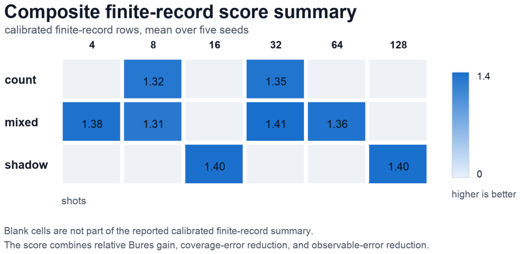
Figure A1 asks whether Bures-distance gains, coverage-error reductions, and observable-error reductions appear in the same measurement cells. The figure is computed from the calibrated finite-record summary, using the same row-wise Bures-vs-best-non-Bures comparison as the additional regime tables. It gives the visual analogue of Table A2 and Table A3: the numerical tables show the individual metrics, while the heatmap shows where the three reductions co-occur.
Figure A1.
Composite measurement-regime summary. Color encodes a combined finite-record score using relative Bures-distance gain, coverage-error reduction, and held-out observable-error reduction. The displayed cells are the calibrated finite-record rows entering this summary.
Figure A1.
Composite measurement-regime summary. Color encodes a combined finite-record score using relative Bures-distance gain, coverage-error reduction, and held-out observable-error reduction. The displayed cells are the calibrated finite-record rows entering this summary.
Appendix G.2. Runtime and Tradeoff Views
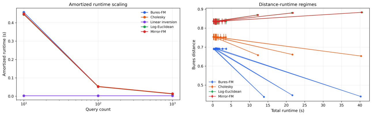
Figure A2 combines the two runtime diagnostics. The left panel asks how amortized inference cost changes as more posterior queries are made. The right panel asks how dense posterior quality and total runtime trade off across geometry choices. Together, the panels show that the learned samplers amortize training cost over repeated posterior queries, while the Bures-geometric sampler occupies a lower-distance region among the implemented geometry controls.
Figure A2.
Supplementary runtime diagnostics. Left: amortized runtime per query as posterior-query count increases. Learned posterior samplers amortize the one-time training cost, while linear inversion remains a point-estimation reference. Right: Bures distance versus total runtime for the implemented geometry and coordinate controls.
Figure A2.
Supplementary runtime diagnostics. Left: amortized runtime per query as posterior-query count increases. Learned posterior samplers amortize the one-time training cost, while linear inversion remains a point-estimation reference. Right: Bures distance versus total runtime for the implemented geometry and coordinate controls.
Appendix G.3. Credible-Ball Coverage
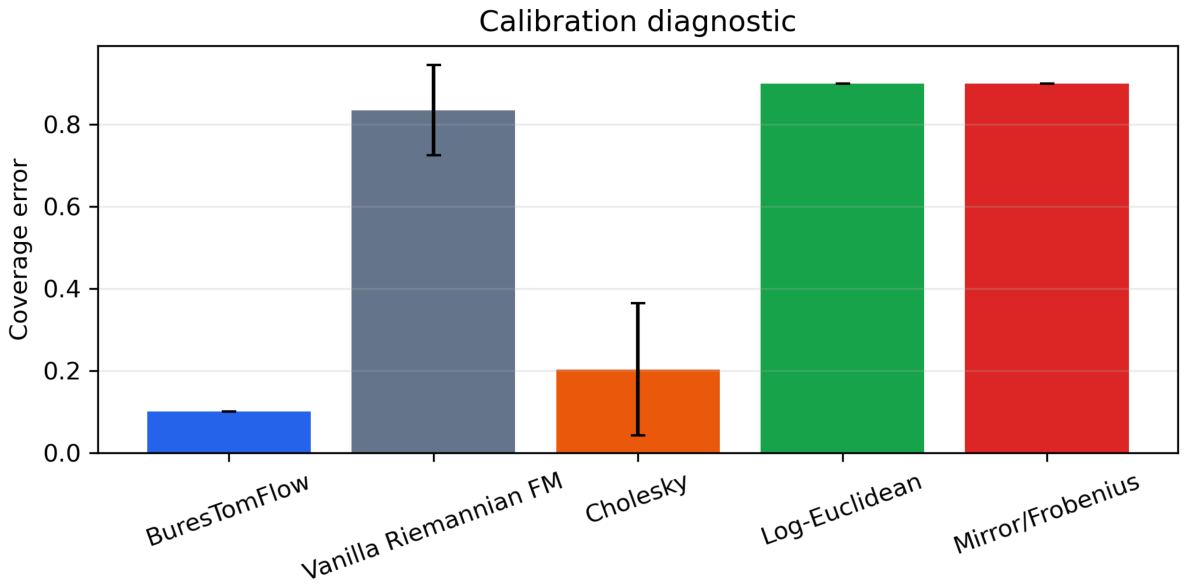
Figure A3 asks whether the posterior sample clouds are calibrated, not merely close in Bures distance. The figure uses the same calibrated finite-record comparison as the main geometry table and reports coverage error for the posterior-sampler baselines. Linear inversion remains outside this comparison because it is a point estimator and does not generate a posterior cloud.
Figure A3.
Coverage-error comparison across posterior-sampler baselines. Lower coverage error indicates closer agreement between nominal credible-ball level and empirical coverage.
Figure A3.
Coverage-error comparison across posterior-sampler baselines. Lower coverage error indicates closer agreement between nominal credible-ball level and empirical coverage.
Appendix G.4. Bures-Localized Rank Calibration
Figure A4 asks whether the calibration ordering is directionally consistent under a Bures-local posterior-rank probe. The figure and Table A4 use the calibrated finite-record posterior samples and compare ACLD, 10-bin ECE, and the KS statistic. This diagnostic complements the credible-ball coverage figure by probing posterior mass through random Bures balls around independent anchor states.
Figure A4.
Bures-localized rank-calibration check inspired by conditional localization and simulation-based calibration. Lower ACLD and lower 10-bin rank ECE indicate better comparative posterior-rank behavior under the same calibrated finite-record scenarios.
Figure A4.
Bures-localized rank-calibration check inspired by conditional localization and simulation-based calibration. Lower ACLD and lower 10-bin rank ECE indicate better comparative posterior-rank behavior under the same calibrated finite-record scenarios.
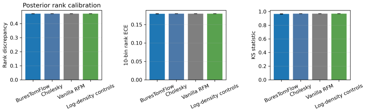
Table A4.
Rank-calibration results on calibrated finite-record scenarios. Lower is better for ACLD and 10-bin ECE. The accompanying figure also reports the KS statistic. This table keeps the two most compact rank-summary columns. Log-density controls aggregate two coordinate-control variants.
Table A4.
Rank-calibration results on calibrated finite-record scenarios. Lower is better for ACLD and 10-bin ECE. The accompanying figure also reports the KS statistic. This table keeps the two most compact rank-summary columns. Log-density controls aggregate two coordinate-control variants.
| Method | Evaluation scale | Rank calibration ↓ | ||
| Scenarios | Rank samples | ACLD | 10-bin ECE | |
| BuresTomFlow | 40 | 51,200 | ||
| Cholesky | 40 | 51,200 | ||
| Vanilla RFM | 40 | 51,200 | ||
| Log-density controls | 80 | 102,400 | ||
Appendix G.5. Bures-Kernel Scaling
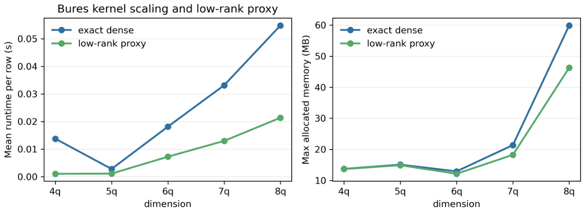
Figure A5 asks a narrower supporting question: whether Bures kernel operations and a spectral low-rank proxy remain computationally tractable in larger matrix dimensions. The figure comes from the standalone Bures-kernel scaling diagnostic and compares exact dense operations with a low-rank proxy in runtime and memory. It supports the feasibility of the geometric component beyond the dense four-qubit training benchmark.
Figure A5.
Bures-kernel scaling and spectral low-rank proxy study. Exact dense Bures operations complete up to the 8-qubit kernel-operation diagnostic shown here, while the low-rank proxy reduces runtime and memory in this diagnostic. The study concerns the geometry kernel used by the sampler.
Figure A5.
Bures-kernel scaling and spectral low-rank proxy study. Exact dense Bures operations complete up to the 8-qubit kernel-operation diagnostic shown here, while the low-rank proxy reduces runtime and memory in this diagnostic. The study concerns the geometry kernel used by the sampler.
Appendix H. Scope and Limitations
The evidence in this appendix supports the paper’s stated claim: Bures-geometric posterior sampling improves the tested dense finite-record tomography regimes while preserving calibrated posterior uncertainty better than the geometry controls. The experiments use exact dense four-qubit density matrices, finite count/mixed/shadow records, and posterior summaries formed from a finite number of learned samples. Within this scope, the method is evaluated against geometry and coordinate controls that isolate the role of the Bures path and tangent loss.
The present dense implementation keeps the full density matrix explicit. This choice makes the geometry and posterior metrics directly measurable: trace, positivity, Bures distance, held-out observables, credible-ball coverage, and rank calibration can all be evaluated without replacing the density matrix by a compressed ansatz. The same choice also fixes the computational scope. Larger Hilbert spaces require either structured state families, low-rank parameterizations, tensor-network structure, or additional approximations to the Bures kernel. Figure A5 studies one such geometric kernel proxy, but the main posterior-tomography claim remains the dense finite-record result reported in the tables.
The measurement model is likewise controlled. The records come from ideal product-Pauli Born sampling, with finite-shot ambiguity but without device noise, drift, or adaptive measurement design. This is the right setting for isolating whether Bures geometry improves posterior sampling under finite records. Extending the sampler to noisy measurement channels, adaptive protocols, and experimentally collected records is a separate evaluation problem. The appendix is organized to make this separation explicit: protocol and geometry first, metrics and calibration second, then evidence tables and computational diagnostics.
NeurIPS Paper Checklist
- 1.
-
ClaimsQuestion: Do the main claims made in the abstract and introduction accurately reflect the paper’s contributions and scope?Answer: [Yes]Justification: The abstract and introduction state the finite-record posterior tomography setting, the Bures-geometric Flow Matching construction, and the dense four-qubit experimental scope. The scope and limitations are further stated in Appendix H.Guidelines:
- The answer [N/A] means that the abstract and introduction do not include the claims made in the paper.
- The abstract and/or introduction should clearly state the claims made, including the contributions made in the paper and important assumptions and limitations. A [No] or [N/A] answer to this question will not be perceived well by the reviewers.
- The claims made should match theoretical and experimental results, and reflect how much the results can be expected to generalize to other settings.
- It is fine to include aspirational goals as motivation as long as it is clear that these goals are not attained by the paper.
- 2.
-
LimitationsQuestion: Does the paper discuss the limitations of the work performed by the authors?Answer: [Yes]Justification: The paper discusses the dense four-qubit setting, ideal product-Pauli measurement model, and computational scaling in Appendix H. These statements delimit the empirical claims without weakening the reported Bures-path-flow advantage in the evaluated regimes.Guidelines:
- The answer [N/A] means that the paper has no limitation while the answer [No] means that the paper has limitations, but those are not discussed in the paper.
- The authors are encouraged to create a separate “Limitations” section in their paper.
- The paper should point out any strong assumptions and how robust the results are to violations of these assumptions (e.g., independence assumptions, noiseless settings, model well-specification, asymptotic approximations only holding locally). The authors should reflect on how these assumptions might be violated in practice and what the implications would be.
- The authors should reflect on the scope of the claims made, e.g., if the approach was only tested on a few datasets or with a few runs. In general, empirical results often depend on implicit assumptions, which should be articulated.
- The authors should reflect on the factors that influence the performance of the approach. For example, a facial recognition algorithm may perform poorly when image resolution is low or images are taken in low lighting. Or a speech-to-text system might not be used reliably to provide closed captions for online lectures because it fails to handle technical jargon.
- The authors should discuss the computational efficiency of the proposed algorithms and how they scale with dataset size.
- If applicable, the authors should discuss possible limitations of their approach to address problems of privacy and fairness.
- While the authors might fear that complete honesty about limitations might be used by reviewers as grounds for rejection, a worse outcome might be that reviewers discover limitations that aren’t acknowledged in the paper. The authors should use their best judgment and recognize that individual actions in favor of transparency play an important role in developing norms that preserve the integrity of the community. Reviewers will be specifically instructed to not penalize honesty concerning limitations.
- 3.
-
Theory assumptions and proofsQuestion: For each theoretical result, does the paper provide the full set of assumptions and a complete (and correct) proof?Answer: [N/A]Justification: The paper does not claim new formal theorems. Appendix B states the known Bures-Wasserstein construction and cites the relevant geometry references.Guidelines:
- The answer [N/A] means that the paper does not include theoretical results.
- All the theorems, formulas, and proofs in the paper should be numbered and cross-referenced.
- All assumptions should be clearly stated or referenced in the statement of any theorems.
- The proofs can either appear in the main paper or the supplemental material, but if they appear in the supplemental material, the authors are encouraged to provide a short proof sketch to provide intuition.
- Inversely, any informal proof provided in the core of the paper should be complemented by formal proofs provided in appendix or supplemental material.
- Theorems and Lemmas that the proof relies upon should be properly referenced.
- 4.
-
Experimental result reproducibilityQuestion: Does the paper fully disclose all the information needed to reproduce the main experimental results of the paper to the extent that it affects the main claims and/or conclusions of the paper (regardless of whether the code and data are provided or not)?Answer: [Yes]Justification: Appendices Appendix A, Appendix C, and Appendix D specify the simulator, measurement records, model components, optimizer, posterior sampling, metrics, and calibration protocol needed to reproduce the main comparisons.Guidelines:
- The answer [N/A] means that the paper does not include experiments.
- If the paper includes experiments, a [No] answer to this question will not be perceived well by the reviewers: Making the paper reproducible is important, regardless of whether the code and data are provided or not.
- If the contribution is a dataset and/or model, the authors should describe the steps taken to make their results reproducible or verifiable.
- Depending on the contribution, reproducibility can be accomplished in various ways. For example, if the contribution is a novel architecture, describing the architecture fully might suffice, or if the contribution is a specific model and empirical evaluation, it may be necessary to either make it possible for others to replicate the model with the same dataset, or provide access to the model. In general. releasing code and data is often one good way to accomplish this, but reproducibility can also be provided via detailed instructions for how to replicate the results, access to a hosted model (e.g., in the case of a large language model), releasing of a model checkpoint, or other means that are appropriate to the research performed.
-
While NeurIPS does not require releasing code, the conference does require all submissions to provide some reasonable avenue for reproducibility, which may depend on the nature of the contribution. For example
- (a)
- If the contribution is primarily a new algorithm, the paper should make it clear how to reproduce that algorithm.
- (b)
- If the contribution is primarily a new model architecture, the paper should describe the architecture clearly and fully.
- (c)
- If the contribution is a new model (e.g., a large language model), then there should either be a way to access this model for reproducing the results or a way to reproduce the model (e.g., with an open-source dataset or instructions for how to construct the dataset).
- (d)
- We recognize that reproducibility may be tricky in some cases, in which case authors are welcome to describe the particular way they provide for reproducibility. In the case of closed-source models, it may be that access to the model is limited in some way (e.g., to registered users), but it should be possible for other researchers to have some path to reproducing or verifying the results.
- 5.
-
Open access to data and codeQuestion: Does the paper provide open access to the data and code, with sufficient instructions to faithfully reproduce the main experimental results, as described in supplemental material?Answer: [No]Justification: The current anonymous submission does not provide an open code or data archive. The experimental data are synthetic and generated by the protocol described in the appendix; an anonymized or final release can be prepared separately if the authors choose to release the implementation.Guidelines:
- The answer [N/A] means that paper does not include experiments requiring code.
- Please see the NeurIPS code and data submission guidelines (https://neurips.cc/public/guides/CodeSubmissionPolicy) for more details.
- While we encourage the release of code and data, we understand that this might not be possible, so [No] is an acceptable answer. Papers cannot be rejected simply for not including code, unless this is central to the contribution (e.g., for a new open-source benchmark).
- The instructions should contain the exact command and environment needed to run to reproduce the results. See the NeurIPS code and data submission guidelines (https://neurips.cc/public/guides/CodeSubmissionPolicy) for more details.
- The authors should provide instructions on data access and preparation, including how to access the raw data, preprocessed data, intermediate data, and generated data, etc.
- The authors should provide scripts to reproduce all experimental results for the new proposed method and baselines. If only a subset of experiments are reproducible, they should state which ones are omitted from the script and why.
- At submission time, to preserve anonymity, the authors should release anonymized versions (if applicable).
- Providing as much information as possible in supplemental material (appended to the paper) is recommended, but including URLs to data and code is permitted.
- 6.
-
Experimental setting/detailsQuestion: Does the paper specify all the training and test details (e.g., data splits, hyperparameters, how they were chosen, type of optimizer) necessary to understand the results?Answer: [Yes]Justification: Appendices Appendix A, Appendix C, Appendix D, and Appendix F specify the data generation, training details, model hyperparameters, posterior sampling settings, evaluation splits, and measurement regimes.Guidelines:
- The answer [N/A] means that the paper does not include experiments.
- The experimental setting should be presented in the core of the paper to a level of detail that is necessary to appreciate the results and make sense of them.
- The full details can be provided either with the code, in appendix, or as supplemental material.
- 7.
-
Experiment statistical significanceQuestion: Does the paper report error bars suitably and correctly defined or other appropriate information about the statistical significance of the experiments?Answer: [Yes]Justification: The main and supplementary result tables report variability across repeated runs, and Appendix D defines the reporting and calibration quantities used to interpret those comparisons.Guidelines:
- The answer [N/A] means that the paper does not include experiments.
- The authors should answer [Yes] if the results are accompanied by error bars, confidence intervals, or statistical significance tests, at least for the experiments that support the main claims of the paper.
- The factors of variability that the error bars are capturing should be clearly stated (for example, train/test split, initialization, random drawing of some parameter, or overall run with given experimental conditions).
- The method for calculating the error bars should be explained (closed form formula, call to a library function, bootstrap, etc.)
- The assumptions made should be given (e.g., Normally distributed errors).
- It should be clear whether the error bar is the standard deviation or the standard error of the mean.
- It is OK to report 1-sigma error bars, but one should state it. The authors should preferably report a 2-sigma error bar than state that they have a 96% CI, if the hypothesis of Normality of errors is not verified.
- For asymmetric distributions, the authors should be careful not to show in tables or figures symmetric error bars that would yield results that are out of range (e.g., negative error rates).
- If error bars are reported in tables or plots, the authors should explain in the text how they were calculated and reference the corresponding figures or tables in the text.
- 8.
-
Experiments compute resourcesQuestion: For each experiment, does the paper provide sufficient information on the computer resources (type of compute workers, memory, time of execution) needed to reproduce the experiments?Answer: [No]Justification: The paper reports runtime evidence, but it does not fully enumerate the hardware, memory, and total compute used for every experiment. The compute environment was heterogeneous, so a complete per-run resource accounting is not included in the current manuscript.Guidelines:
- The answer [N/A] means that the paper does not include experiments.
- The paper should indicate the type of compute workers CPU or GPU, internal cluster, or cloud provider, including relevant memory and storage.
- The paper should provide the amount of compute required for each of the individual experimental runs as well as estimate the total compute.
- The paper should disclose whether the full research project required more compute than the experiments reported in the paper (e.g., preliminary or failed experiments that didn’t make it into the paper).
- 9.
-
Code of ethicsQuestion: Does the research conducted in the paper conform, in every respect, with the NeurIPS Code of Ethics https://neurips.cc/public/EthicsGuidelines?Answer: [Yes]Justification: The study uses synthetic quantum-tomography simulations and does not involve human subjects, private data, deployed decision systems, or other settings that would require a deviation from the NeurIPS Code of Ethics.Guidelines:
- The answer [N/A] means that the authors have not reviewed the NeurIPS Code of Ethics.
- If the authors answer [No], they should explain the special circumstances that require a deviation from the Code of Ethics.
- The authors should make sure to preserve anonymity (e.g., if there is a special consideration due to laws or regulations in their jurisdiction).
- 10.
-
Broader impactsQuestion: Does the paper discuss both potential positive societal impacts and negative societal impacts of the work performed?Answer: [N/A]Justification: The work is foundational methodology for synthetic quantum-state tomography and is not tied to a deployed application or a direct societal-impact pathway in the paper.Guidelines:
- The answer [N/A] means that there is no societal impact of the work performed.
- If the authors answer [N/A] or [No], they should explain why their work has no societal impact or why the paper does not address societal impact.
- Examples of negative societal impacts include potential malicious or unintended uses (e.g., disinformation, generating fake profiles, surveillance), fairness considerations (e.g., deployment of technologies that could make decisions that unfairly impact specific groups), privacy considerations, and security considerations.
- The conference expects that many papers will be foundational research and not tied to particular applications, let alone deployments. However, if there is a direct path to any negative applications, the authors should point it out. For example, it is legitimate to point out that an improvement in the quality of generative models could be used to generate Deepfakes for disinformation. On the other hand, it is not needed to point out that a generic algorithm for optimizing neural networks could enable people to train models that generate Deepfakes faster.
- The authors should consider possible harms that could arise when the technology is being used as intended and functioning correctly, harms that could arise when the technology is being used as intended but gives incorrect results, and harms following from (intentional or unintentional) misuse of the technology.
- If there are negative societal impacts, the authors could also discuss possible mitigation strategies (e.g., gated release of models, providing defenses in addition to attacks, mechanisms for monitoring misuse, mechanisms to monitor how a system learns from feedback over time, improving the efficiency and accessibility of ML).
- 11.
-
SafeguardsQuestion: Does the paper describe safeguards that have been put in place for responsible release of data or models that have a high risk for misuse (e.g., pre-trained language models, image generators, or scraped datasets)?Answer: [N/A]Justification: The paper does not release a high-risk model, scraped dataset, or dual-use asset requiring release safeguards.Guidelines:
- The answer [N/A] means that the paper poses no such risks.
- Released models that have a high risk for misuse or dual-use should be released with necessary safeguards to allow for controlled use of the model, for example by requiring that users adhere to usage guidelines or restrictions to access the model or implementing safety filters.
- Datasets that have been scraped from the Internet could pose safety risks. The authors should describe how they avoided releasing unsafe images.
- We recognize that providing effective safeguards is challenging, and many papers do not require this, but we encourage authors to take this into account and make a best faith effort.
- 12.
-
Licenses for existing assetsQuestion: Are the creators or original owners of assets (e.g., code, data, models), used in the paper, properly credited and are the license and terms of use explicitly mentioned and properly respected?Answer: [Yes]Justification: The implementation uses the public flow_matching package credited by Lipman et al.(2024)Lipman, Havasi, Holderrieth, Shaul, Le, Karrer, Chen, Lopez-Paz, Ben-Hamu, and Gat [22]; its repository states that the code is distributed under the CC BY-NC 4.0 license. The experiments use synthetic data generated by the stated protocol rather than an external dataset.Guidelines:
- The answer [N/A] means that the paper does not use existing assets.
- The authors should cite the original paper that produced the code package or dataset.
- The authors should state which version of the asset is used and, if possible, include a URL.
- The name of the license (e.g., CC-BY 4.0) should be included for each asset.
- For scraped data from a particular source (e.g., website), the copyright and terms of service of that source should be provided.
- If assets are released, the license, copyright information, and terms of use in the package should be provided. For popular datasets, paperswithcode.com/datasets has curated licenses for some datasets. Their licensing guide can help determine the license of a dataset.
- For existing datasets that are re-packaged, both the original license and the license of the derived asset (if it has changed) should be provided.
- If this information is not available online, the authors are encouraged to reach out to the asset’s creators.
- 13.
-
New assetsQuestion: Are new assets introduced in the paper well documented and is the documentation provided alongside the assets?Answer: [N/A]Justification: The paper does not introduce or release a new dataset, benchmark asset, model checkpoint, or software package as part of the submission.Guidelines:
- The answer [N/A] means that the paper does not release new assets.
- Researchers should communicate the details of the dataset/code/model as part of their submissions via structured templates. This includes details about training, license, limitations, etc.
- The paper should discuss whether and how consent was obtained from people whose asset is used.
- At submission time, remember to anonymize your assets (if applicable). You can either create an anonymized URL or include an anonymized zip file.
- 14.
-
Crowdsourcing and research with human subjectsQuestion: For crowdsourcing experiments and research with human subjects, does the paper include the full text of instructions given to participants and screenshots, if applicable, as well as details about compensation (if any)?Answer: [N/A]Justification: The paper does not involve crowdsourcing or research with human subjects.Guidelines:
- The answer [N/A] means that the paper does not involve crowdsourcing nor research with human subjects.
- Including this information in the supplemental material is fine, but if the main contribution of the paper involves human subjects, then as much detail as possible should be included in the main paper.
- According to the NeurIPS Code of Ethics, workers involved in data collection, curation, or other labor should be paid at least the minimum wage in the country of the data collector.
- 15.
-
Institutional review board (IRB) approvals or equivalent for research with human subjectsQuestion: Does the paper describe potential risks incurred by study participants, whether such risks were disclosed to the subjects, and whether Institutional Review Board (IRB) approvals (or an equivalent approval/review based on the requirements of your country or institution) were obtained?Answer: [N/A]
- 15.
-
Justification: The paper does not involve crowdsourcing or research with human subjects, so IRB approval or an equivalent review is not applicable.Guidelines:
- The answer [N/A] means that the paper does not involve crowdsourcing nor research with human subjects.
- Depending on the country in which research is conducted, IRB approval (or equivalent) may be required for any human subjects research. If you obtained IRB approval, you should clearly state this in the paper.
- We recognize that the procedures for this may vary significantly between institutions and locations, and we expect authors to adhere to the NeurIPS Code of Ethics and the guidelines for their institution.
- For initial submissions, do not include any information that would break anonymity (if applicable), such as the institution conducting the review.
- 16.
-
Declaration of LLM usageQuestion: Does the paper describe the usage of LLMs if it is an important, original, or non-standard component of the core methods in this research? Note that if the LLM is used only for writing, editing, or formatting purposes and does not impact the core methodology, scientific rigor, or originality of the research, declaration is not required.Answer: [N/A]Justification: LLMs are not an important, original, or non-standard component of the core method or experiments in this research.Guidelines:
- The answer [N/A] means that the core method development in this research does not involve LLMs as any important, original, or non-standard components.
- Please refer to our LLM policy in the NeurIPS handbook for what should or should not be described.
References
- Aaronson, Scott. Shadow tomography of quantum states. In Proceedings of the 50th Annual ACM SIGACT Symposium on Theory of Computing (STOC), 2018; pp. 325–338. [Google Scholar] [CrossRef]
- Ahmed, Shahnawaz; Sánchez Muñoz, Carlos; Nori, Franco; Frisk Kockum, Anton. Quantum state tomography with conditional generative adversarial networks. Phys. Rev. Lett. 2021, 127, 140502. [Google Scholar] [CrossRef]
- Albergo, Michael S.; Boffi, Nicholas M.; Vanden-Eijnden, Eric. Stochastic interpolants: A unifying framework for flows and diffusions. J. Mach. Learn. Res. 2025, 26(209), 1–80. Available online: https://jmlr.org/papers/v26/23-1605.html.
- Bhatia, Rajendra; Jain, Tanvi; Lim, Yongdo. On the Bures-Wasserstein distance between positive definite matrices. Expo. Math. 2019, 37(2), 165–191. [Google Scholar] [CrossRef]
- Blume-Kohout, Robin. Optimal, reliable estimation of quantum states. New J. Phys. 2010, 12, 043034. [Google Scholar] [CrossRef]
- Braunstein, Samuel L.; Caves, Carlton M. Statistical distance and the geometry of quantum states. Phys. Rev. Lett. 1994, 72(22), 3439–3443. [Google Scholar] [CrossRef]
- Bures, Donald. An extension of Kakutani’s theorem on infinite product measures to the tensor product of semifinite W*-algebras. Trans. Am. Math. Soc. 1969, 135, 199–212. [Google Scholar] [CrossRef]
- Carrasquilla, Juan; Torlai, Giacomo; Melko, Roger G.; Aolita, Leandro. Reconstructing quantum states with generative models. Nat. Mach. Intell. 2019, 1, 155–161. [Google Scholar] [CrossRef]
- Cha, Peter J.; Ginsparg, Paul; Wu, Felix; Carrasquilla, Juan; McMahon, Peter L.; Kim, Eun-Ah. Attention-based quantum tomography. Mach. Learn. Sci. Technol. 2022, 3(1), 01LT01. [Google Scholar] [CrossRef]
- Chen, Ricky T. Q.; Lipman, Yaron. Flow matching on general geometries. International Conference on Learning Representations, 2024; Available online: https://openreview.net/forum?id=g7ohDlTITL.
- Chen, Tianyu; Bansal, Vansh; Scott, James G. CoLT: The conditional localization test for assessing the accuracy of neural posterior estimates. In Advances in Neural Information Processing Systems; 2025; Available online: https://openreview.net/forum?id=761hggw1Wx.
- Collas, Antoine; Ju, Ce; Salvy, Nicolas; Thirion, Bertrand. Riemannian flow matching for brain connectivity matrices via pullback geometry. Advances in Neural Information Processing Systems. 2025. Available online: https://openreview.net/forum?id=NY3LzmUXl7.
- Cranmer, Kyle; Brehmer, Johann; Louppe, Gilles. The frontier of simulation-based inference. Proc. Natl. Acad. Sci. 2020, 117(48), 30055–30062. [Google Scholar] [CrossRef]
- Elben, Andreas; Flammia, Steven T.; Huang, Hsin-Yuan; Kueng, Richard; Preskill, John; Vermersch, Benoît; Zoller, Peter. The randomized measurement toolbox. Nat. Rev. Phys. 2023, 5, 9–24. [Google Scholar] [CrossRef]
- Granade, Christopher; Combes, Joshua; Cory, D. G. Practical Bayesian tomography. New J. Phys. 2016, 18, 033024. [Google Scholar] [CrossRef]
- Gross, David; Liu, Yi-Kai; Flammia, Steven T.; Becker, Stephen; Eisert, Jens. Quantum state tomography via compressed sensing. Phys. Rev. Lett. 2010, 105, 150401. [Google Scholar] [CrossRef]
- Hradil, Zdeněk. Quantum-state estimation. Phys. Rev. A 1997, 55(3), R1561–R1564. [Google Scholar] [CrossRef]
- Huang, Hsin-Yuan; Kueng, Richard; Preskill, John. Predicting many properties of a quantum system from very few measurements. Nat. Phys. 2020, 16(10), 1050–1057. [Google Scholar] [CrossRef]
- Jozsa, Richard. Fidelity for mixed quantum states. J. Mod. Opt. 1994, 41(12), 2315–2323. [Google Scholar] [CrossRef]
- Lee, Juho; Lee, Yoonho; Kim, Jungtaek; Kosiorek, Adam; Choi, Seungjin; Teh, Yee Whye. Set transformer: A framework for attention-based permutation-invariant neural networks. In Proceedings of the 36th International Conference on Machine Learning, 2019; pp. 3744–3753. Available online: http://proceedings.mlr.press/v97/lee19d.html.
- Lipman, Yaron; Chen, Ricky T. Q.; Ben-Hamu, Heli; Nickel, Maximilian; Le, Matt. Flow matching for generative modeling. International Conference on Learning Representations, 2023; Available online: https://openreview.net/forum?id=PqvMRDCJT9t.
- Lipman, Yaron; Havasi, Marton; Holderrieth, Peter; Shaul, Neta; Le, Matt; Karrer, Brian; Chen, Ricky T. Q.; Lopez-Paz, David; Ben-Hamu, Heli; Gat, Itai. Flow matching guide and code, 2024. Available online: https://arxiv.org/abs/2412.06264.
- Liu, Xingchao; Gong, Chengyue; Liu, Qiang. Flow straight and fast: Learning to generate and transfer data with rectified flow. International Conference on Learning Representations, 2023; Available online: https://openreview.net/forum?id=XVjTT1nw5z.
- Ouyang, Wenzhe; Ye, Qi; Wang, Jinghua; Xu, Zenglin; Chen, Jiming. RFMPose: Generative category-level object pose estimation via riemannian flow matching. Advances in Neural Information Processing Systems. 2025. Available online: https://openreview.net/forum?id=6aaixHco6C.
- Paris, Matteo G. A.; Rehacek, Jaroslav (Eds.) Quantum State Estimation; Springer, 2004; volume 649. [Google Scholar] [CrossRef]
- Sachdev, Subir. Quantum Phase Transitions, 2 edition; Cambridge University Press, 2011. [Google Scholar] [CrossRef]
- Schmale, Tobias; Reh, Moritz; Gärttner, Martin. Efficient quantum state tomography with convolutional neural networks. npj Quantum Inf. 2022, 8, 115. [Google Scholar] [CrossRef]
- Talts, Sean; Betancourt, Michael; Simpson, Daniel; Vehtari, Aki; Gelman, Andrew. Validating Bayesian inference algorithms with simulation-based calibration. 2018. [Google Scholar]
- Tang, Yehui; Long, Mabiao; Yan, Junchi. QuaDiM: A conditional diffusion model for quantum state property estimation. International Conference on Learning Representations, 2025; Available online: https://openreview.net/forum?id=P7f55HQtV8.
- Tong, Alexander; Fatras, Kilian; Malkin, Nikolay; Huguet, Guillaume; Zhang, Yanlei; Rector-Brooks, Jarrid; Wolf, Guy; Bengio, Yoshua. Improving and generalizing flow-based generative models with minibatch optimal transport. Transactions on Machine Learning Research. 2024. Available online: https://openreview.net/forum?id=CD9Snc73AW.
- Torlai, Giacomo; Mazzola, Guglielmo; Carrasquilla, Juan; Troyer, Matthias; Melko, Roger; Carleo, Giuseppe. Neural-network quantum state tomography. Nat. Phys. 2018, 14, 447–450. [Google Scholar] [CrossRef]
- Uhlmann, Armin. The transition probability in the state space of a *-algebra. Rep. Math. Phys. 1976, 9(2), 273–279. [Google Scholar] [CrossRef]
- van Oostrum, Jesse. Bures–wasserstein geometry for positive-definite hermitian matrices and their trace-one subset. Inf. Geom. 2022, 5(2), 405–425. [Google Scholar] [CrossRef]
- Wildberger, Jonas Bernhard; Dax, Maximilian; Buchholz, Simon; Green, Stephen R.; Macke, Jakob H.; Schölkopf, Bernhard. Flow matching for scalable simulation-based inference. Adv. Neural Inf. Process. Syst. 2023, volume 36, pages 16837–16864. Available online: https://proceedings.neurips.cc/paper_files/paper/2023/hash/3663ae53ec078860bb0b9c6606e092a0-Abstract-Conference.html.
- Zhu, Yuchen; Chen, Tianrong; Theodorou, Evangelos A.; Chen, Xie; Tao, Molei. Quantum state generation with structure-preserving diffusion model. 2024. [Google Scholar] [CrossRef]
Figure 1.
Overview of BuresTomFlow. A finite tomography record conditions a neural velocity field. Base density matrices are transported through Bures-Wasserstein paths, then the trained ODE sampler returns physical posterior samples whose quality is checked by Bures distance, coverage error, observable error, and runtime.
Figure 1.
Overview of BuresTomFlow. A finite tomography record conditions a neural velocity field. Base density matrices are transported through Bures-Wasserstein paths, then the trained ODE sampler returns physical posterior samples whose quality is checked by Bures distance, coverage error, observable error, and runtime.
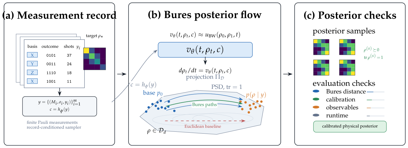
Figure 2.
Measurement-regime analysis. Top: the complete three-family, six-budget sweep, reporting relative Bures-distance reduction and mean reductions in Bures distance, coverage error, and held-out observable error. Bottom: the finite-record summary, reporting Bures distance, posterior coverage, held-out observable error, and runtime-quality tradeoff with seed-level points and regime means.
Figure 2.
Measurement-regime analysis. Top: the complete three-family, six-budget sweep, reporting relative Bures-distance reduction and mean reductions in Bures distance, coverage error, and held-out observable error. Bottom: the finite-record summary, reporting Bures distance, posterior coverage, held-out observable error, and runtime-quality tradeoff with seed-level points and regime means.
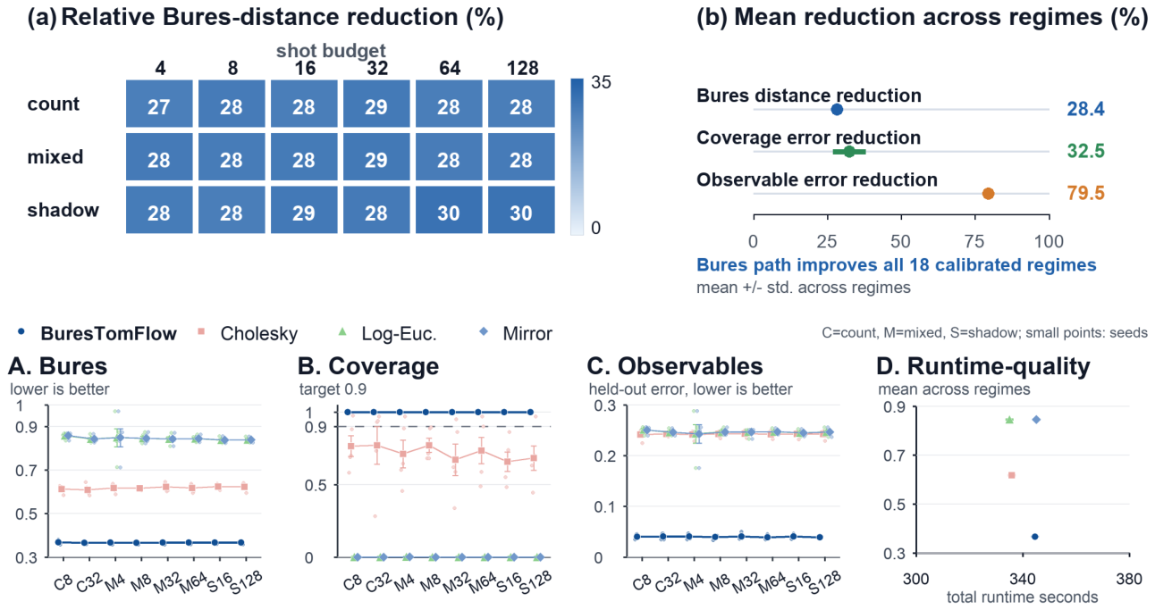
Table 1.
Calibrated finite-record geometry-baseline comparison. Lower is better for Bures distance, coverage error, observable error, and runtime. Values are mean ± standard deviation across eight finite-record regimes with five seeds each. BuresTomFlow has the best Bures distance, coverage error, and observable error among the posterior-sampler baselines.
Table 1.
Calibrated finite-record geometry-baseline comparison. Lower is better for Bures distance, coverage error, observable error, and runtime. Values are mean ± standard deviation across eight finite-record regimes with five seeds each. BuresTomFlow has the best Bures distance, coverage error, and observable error among the posterior-sampler baselines.
| Method | Runs | Posterior quality ↓ | Cost ↓ | ||
| Bures distance | Coverage error | Obs. error | Runtime (s) | ||
| BuresTomFlow | 40 | ||||
| Cholesky geometry | 40 | ||||
| Vanilla Riemannian FM | 40 | ||||
| Log-density chart controls | 80 | ||||
| Linear inversion | 40 | n/a | |||
Disclaimer/Publisher’s Note: The statements, opinions and data contained in all publications are solely those of the individual author(s) and contributor(s) and not of MDPI and/or the editor(s). MDPI and/or the editor(s) disclaim responsibility for any injury to people or property resulting from any ideas, methods, instructions or products referred to in the content. |
© 2026 by the authors. Licensee MDPI, Basel, Switzerland. This article is an open access article distributed under the terms and conditions of the Creative Commons Attribution (CC BY) license (http://creativecommons.org/licenses/by/4.0/).
Copyright: This open access article is published under a Creative Commons CC BY 4.0 license, which permit the free download, distribution, and reuse, provided that the author and preprint are cited in any reuse.