
Submitted:
06 November 2026
Posted:
10 November 2026
You are already at the latest version
Abstract
Design, implementation and control of mineral processing systems are complex processes requiring accurate decision making that often needs to be real-time. In certain cases, the problems can be described by a single function or criterion. However, most often, multiple criteria are involved, often mutually non-aligned or even conflicting. Selection of a flotation collector is a distinctive multicriteria problem where the decision-making problem must be completed even with imprecise, uncertain or unverified/missing data. The paper considers three different rough set approaches for the process of selection of a flotation collector for the rougher flotation of copper minerals. First is the dominance-based rough set approach (DRSA), second a rough-fuzzy approach and the third is a rough-grey approach by rough number-enabled grey relation analysis. The DRSA and the rough-fuzzy approach produced identical ranking of collectors, while the rough-grey approach produced a very similar ranking with reversed positions of the two highest ranked collectors. The results were also compared with PROMETHEE and ELECTRE methods’ results, which were very similar to the rough set-based methods, showing that these approaches can support collector selection in the circumstance of imprecise or uncertain data.
Keywords:
flotation collector selection
; multicriteria decision making
; dominance-based rough set approach (DRSA)
; rough-fuzzy approach
; rough numbers
; grey relation analysis
1. Introduction
The effectiveness of flotation concentration depends largely on the development of flotation reagents, collectors in particular, and on improvements in reagents regime. Improved, most often more selective collectors are continually being developed, leading to the replacement of the traditional xanthates, or their combined use with dithiophosphates, monothiophosphinates, dithiophosphinates, thionocarbamates and thioureas, silica-based Janus nanoparticles, and other compounds [1].
The problem of selecting a collector, a collector type or any flotation reagent is relatively underrepresented in literature, regardless of ore type, for several reasons. According to Nagaraj and Ravishankar [2], reagent selection and optimization is informal, reductionistic and frequently based on personal experience that differs from mineral system or plant to another. The Mining Chemicals Handbook [3] notes that the selection of chemical reagents is often under-appreciated and that proper testing and selection can have a major impact on plant performance. This may seem self-evident, but the limited research reported and the absence of systemic approach suggest otherwise.
An important issue in the selection process is the definition of the problem type and the criteria. In a flotation plant, the problem is generally addressed by laboratory tests that narrow down the list of candidate collectors. In straightforward cases, the next step is to test different dosages and/or combinations of the selected collector(s). However, when there are multiple candidates with different dosages or variable combinations, the problem becomes more complex, not only because of potential unwanted interactions.
The exhaustive list of factors influencing the selection of the optimal collectors needs to be broken down for the purpose of decision making. As Nagaraj [4] states, the important factors, or in decision making terms, the criteria that dictate reagent selection and trade-offs can be decomposed into two classes, technical factors and constraints (Table 1).
Other criteria are certainly worth considering, and the significance of technical factors and constraints can be argued individually. Moreover, the criteria vary from case to case and are strongly determined by the type of tests performed to obtain the information critical for selection. For instance, when determining the preferred collector for multi-stage flotation of a polymetallic sulphide ore, more than one valuable component and more than one type of indicator must be considered. The mere availability of a reagent can also matter.
Another consideration is the goal of the selection process. Rougher flotation tests alone cannot deliver a comprehensive collector selection, because assay, recovery and selectivity, as performance indicators can conflict with one another. Furthermore, selecting any reagent based on rougher flotation alone is difficult, since the decision concerns not only the collector type but also other components of the regime, such as technological position and time of addition. Given this complexity, a decision support system that fully covers the reagents regime, even if only that of collectors, is a matter for multi-objective optimization analysis.
Although multi-criteria decision making (MCDM) methods and their extensions are used relatively often in mining and mineral processing, most often for selecting a mining method [5,6], a waste dump site [7] or a post-mining land use [8], or for assessing terrain stability above underground mining operations [9], only a few studies address collector selection, as confirmed by the extensive review of the state of the art for MCDM in mining and mineral processing Sitorus et al. [10].
Kostović and Gligorić [11] used the fuzzy TOPSIS method to select a collector for lead-zinc sulphide ore flotation and report that the method has potential to be most useful in the final decision-making stage of mineral processing experiments. A study not strictly related to the flotation reagents but concerned with the selection of laboratory reagents [12] employed the Analytic Hierarchy Process (AHP), goal programming, time series analysis and expert systems to rank and select them. The authors argue that the system can serve as a model for purchasing laboratory reagents.
Kursunoglu et al. [13] used the AHP, implemented in Expert Choice 2000 software, to select the acid type for recovering zinc from flotation tailings; the model was built on three criteria and ten sub-criteria. More recently, Xu et al. [14] developed a green comprehensive evaluation system for flotation collectors intended for coal flotation plants, based on AHP coupled with the fuzzy comprehensive evaluation (FCE), while Štirbanović et al. [15] applied the VIKOR method to select the type and dosage of collector in porphyry copper ore rougher flotation, using five criteria. Abdollahi et al. [16] developed a technical-economic framework based on the TOPSIS method for selecting the optimal collector combination in apatite flotation, using five criteria, fixed collector dosages and weights calculated by the entropy method.
Research on rough set-based approaches in mineral processing and mining engineering is limited, and even fewer studies use them as decision support, particularly in hybrid forms such as rough-fuzzy or rough-grey approaches.
In his doctoral dissertation, Štirbanović [17] applied rough set theory to the selection of a flotation collector and a flotation machine and compared the results with those of VIKOR, AHP, ELECTRE, PROMETHEE and TOPSIS.
Rough set theory was applied to select the optimal location for a flotation tailings dump, considering nine conditional attributes and two decision levels, in a direct (non-dominance-based) approach by Štirbanović et al. [18].
Reported applications of the Dominance-based Rough Set Approach (DRSA) to selection problems are also uncommon. Examples from other fields include Boudreau-Trude and Zaras [19] who compared the AHP with the DRSA for selecting investment projects on twenty-four criteria, and Zaras et al. [20], who applied the DRSA to the selection of sustainable development projects, with twenty-nine alternatives and seven attributes. Abastante et al. [21] used the DRSA with ten attributes, to address the location of undesirable facilities such as waste incinerators and landfills.
Hybrid rough-set approaches have been used in several recent studies. Pamučar et al. [22] used a GIS-based multi-criteria hybrid model combining fuzzy and rough numbers for wind farm site selection. Rough Best-Worst Method (BWM) was used for determining the criteria weights, rough Multi Attributive Ideal-Real Comparative Analysis (MAIRCA), for ranking of alternatives, while the fuzzy sets were used for standardization of the criteria. Kousar and Kausar [23] used an integrated fuzzy-rough approach to analyze stakeholder perception of agritourism ranking seven alternatives on ten criteria. Sandra et al. [24] used a fuzzy-rough integrating novel T-Spherical Hesitant Fuzzy Rough Sets (T-SHFR), MEREC-G and RAWEC to select drilling techniques for heat extraction from geothermal reservoirs and compared the results with CODAS, COPRAS, COCOSO, MOORA, PROMETHEE and MCRAT.
Li et al. [25,26] and Bai and Sarkis [27,28] applied grey-based rough decision-making to supplier selection and the evaluation of the supplier development programs.
Particularly interesting is the paper by Zhai et al. [29]. The authors have proposed a procedure for the rough-grey analysis based on the “difference coefficient” to depict the distance between the two rough numbers. The combination of this coefficient and the Grey Relational Analysis (GRA) can serve as a decision support tool that includes features both from the grey approach and rough set theory.
Milisavljević et al. [30] used grey theory as a decision support tool for mining machine selection, and Bakhtavar and Lotfian [31] integrated fuzzy AHP and grey MCDM in a case study of mineral processing plant site selection. Wang et al. [32] used a rough number-grey correlation TOPSIS method to evaluate green suppliers of high-energy consuming enterprises.
The aim of this paper is to demonstrate the use of rough set-based concepts in the mineral processing environment, by applying the Dominance based Rough Set Approach, a hybrid fuzzy-rough and a hybrid rough-grey approach to flotation collector selection.
2. Materials and Methods
2.1. Laboratory Tests
Laboratory flotation tests of copper minerals from an ore deposit in Serbia were performed with six different collectors, with the aim of selecting the optimal collector [33]. The ore was sampled from the conveyor belts in front of the rod mills at the flotation plant of a mine in Serbia that processes this ore, since the tests comprised laboratory grinding and rougher flotation.
The results of the partial chemical analysis are presented in Table 2.
Mineralogical tests were performed on the laboratory-ground ore sample used in the flotation tests. Based on the quantitative mineralogy analysis, the following mineral composition of samples was determined: pyrite, chalcopyrite, covellite, magnetite, rutile, and gangue minerals. Sulfides make up 4.4% of the sample mass, and 91.9% of the sulfide particles are free.
Collector efficiency tests for copper minerals were performed on the ore samples under the following conditions:
- a)
- Of all possible parameters, only the collector was varied;
- b)
- For each of six tested collectors or combinations of collectors, a series of three identical tests was performed;
- c)
- The remaining parameters were held constant:
- weight of representative samples ………………………………………………………………1500 g
- size of representative sample material ………………………………………………….100% -2 mm
- grinding in a ball mill to a fineness of ……………………………………………………60% -74 μm
- pH = ………………………………………………………………………………………………….10.5
- conditioning with 28% of solids ……………………………………………………………t = 10 min
- collector (or collector mixture) consumption …………………………………………..45 g/t of ore
- frother consumption……………………………………………………………………..when needed
- flotation time………………………………………………………………………………….t = 15 min
With these conditions held constant, the copper, gold and sulfur contents were determined in the rougher concentrate of copper minerals and in the underflow (tailings).
Six collectors or collector combinations, presented in Table 3, were tested. For future reference, they are denoted as FCi (Flotation collectors).
The three tests under identical conditions were performed to reliably determine the effect of collector change on the concentrate. The results are presented in tables 4 through 6 [33].

Table 4.
Results of test no. 1 [33].
Table 4.
Results of test no. 1 [33].
| Flotation collector | Cu Rec, % | Cu Assay, % | Au Rec, % | Au Assay, g/t | FeS2 rec, % |
|---|---|---|---|---|---|
| FC1 | 91.520 | 3.275 | 22.570 | 0.461 | 90.080 |
| FC2 | 93.610 | 3.444 | 24.022 | 0.530 | 64.920 |
| FC3 | 95.970 | 2.710 | 29.986 | 0.473 | 88.330 |
| FC4 | 97.250 | 2.490 | 22.617 | 0.469 | 86.580 |
| FC5 | 97.060 | 2.515 | 35.330 | 0.510 | 71.520 |
| FC6 | 97.100 | 2.670 | 34.703 | 0.516 | 63.180 |
Table 5.
Results of test no. 2 [33].
Table 5.
Results of test no. 2 [33].
| Flotation collector | Cu Rec, % | Cu Assay, % | Au Rec, % | Au Assay, g/t | FeS2 rec, % |
|---|---|---|---|---|---|
| FC1 | 92.080 | 3.015 | 22.255 | 0.425 | 95.010 |
| FC2 | 92.600 | 3.560 | 23.757 | 0.587 | 75.510 |
| FC3 | 97.350 | 2.540 | 30.385 | 0.496 | 89.340 |
| FC4 | 95.580 | 2.665 | 22.493 | 0.437 | 88.860 |
| FC5 | 96.290 | 2.770 | 35.362 | 0.517 | 55.650 |
| FC6 | 96.240 | 2.810 | 34.622 | 0.527 | 51.890 |
Table 6.
Results of test no. 3 [33].
Table 6.
Results of test no. 3 [33].
| Flotation collector | Cu Rec, % | Cu Assay, % | Au Rec, % | Au Assay, g/t | FeS2 rec, % |
|---|---|---|---|---|---|
| FC1 | 92.710 | 3.000 | 22.170 | 0.435 | 90.340 |
| FC2 | 95.010 | 4.035 | 23.950 | 0.595 | 49.870 |
| FC3 | 96.210 | 1.925 | 30.260 | 0.535 | 92.410 |
| FC4 | 96.660 | 3.245 | 22.301 | 0.418 | 83.690 |
| FC5 | 96.620 | 2.680 | 35.511 | 0.503 | 61.880 |
| FC6 | 96.560 | 2.770 | 34.594 | 0.512 | 56.660 |
Seven criteria, designated as attributes A1 – A7 were used, recovery of Cu in the rougher concentrate (A1), Cu assay in the rougher concentrate (A2), recovery of Au in the rougher concentrate (A3), Au assay in the rougher concentrate (A4), collector prices (A5), collector toxicity (A6) and selectivity with respect to pyrite expressed as the recovery of pyrite in rougher concentrate (A7). Attributes A1 – A4 and A6 are gain criteria (higher is better) and A5 and A7 are cost criteria (lower is better); toxicity is expressed as LD50 (mg/kg), so a higher value corresponds to a less toxic collector.
It should be noted that the selection process presented here is a technological point of view only, without considering the quantities of the concentrates obtained or their actual value.
To select the optimal collector, the DRSA method was used, together with hybrid approaches combining rough set theory with fuzzy set theory and with grey systems theory. For comparison with conventional MCDM methods, the results of PROMETHEE and ELECTRE were used as well.
The generative AI tool Claude (Anthropic; Claude Sonnet 5.5, accessed October–November 2026) was used (i) to write Python scripts that independently reproduced the calculations of each method and were used to check the results (the scripts, as well as the spreadsheet calculations, were checked against the author’s calculations); and (ii) to review the consistency of the text, tables, equations and cross-references with the calculations. The AI tool was not used to generate data. The author verified all AI-generated content and takes full responsibility for the manuscript. The Python scripts and the Excel workbooks used for the calculations are available from the author on request.
2.2. The DRSA Method
Engineering problems related to decision making can be described by a set of attributes (properties, features) related to the input parameters of the problem or system in question, its output parameters or conditions. Rough set theory is an efficient tool for analysis of problems in which the data are characterized by imprecision, ambiguity or insufficiency. According to the rough set theory, with every input or output parameter of the system or the state observed, a certain amount of information is associated, and this information can be expressed through a number of attributes. Objects having the same description in terms of attributes are called indiscernible with respect to the available information [34,35].
Indiscernibility provides a foundation for dividing the universe into groups of indiscernible objects, called elementary sets, which can be further used in the process of knowledge acquisition. The use of indiscernibility relation results in information granulation, meaning that every subset of the universe can be expressed through these blocks either precisely or approximately. In the case of approximate representation, a set X can be described through two approximations: the lower approximation of X, consisting of every elementary set contained in X, and the upper approximation of X, consisting of all elementary sets having a non-empty intersection with X (the members of these sets may belong to X). The difference between the upper and the lower approximation creates the boundary area of a rough set. For the elements in this area, it cannot be stated with accuracy whether they belong to X or not. Also, the upper and the lower approximations of the division of the universe U into the decision classes makes possible the induction of certain and possible knowledge in the form of decision rules of the type “if… then”.
The area of multi-criteria decision making is particularly suitable for the application of rough sets, since the decision-making process often demands different subjective information such as the weights, substitution rates and various thresholds, and in addition, the decision makers (DMs) often make decisions that cannot be expressed by specific parameters. Moreover, the inconsistency is a common feature of the decision-making process, and therefore rough sets can be considered particularly appropriate for use in this area.
By extending the indiscernibility-based rough set approach, the analysis of preference-ordered data is enabled. This extension, called the Dominance-based Rough Set Approach (DRSA), replaces the indiscernibility relation with a dominance relation in the rough approximation of decision classes. DRSA was developed for problems in which the ordinal evaluation of the objects is known and in which monotonic relationships between these evaluations exist, which is an additional reason for the suitability of DRSA use in problems solved by the multi-criteria analysis techniques [34,35,36].
With DRSA, ranking is based on granules of knowledge generated by the attributes. The granules are dominance cones in the space of attribute values.
Let us consider a finite set of objects A evaluated by a finite set of criteria C. The preference information concerning the multicriteria choice or ranking problem is a data set in the form of a pairwise comparison table which includes pairs of some reference objects from a subset B ⊆ A × A. This is described by preference relations on particular criteria and a comprehensive preference relation [37].
If P ⊆ C is a set of attributes, and subsets are denoted as cardinal criteria (PN), the ordinal criteria (PO) and regular attributes (PR), the pair of objects (x,y) dominates over the pair of objects (w,z) as P ⊆ C (short denomination (x,y) P-dominates (w,z) as (x,y)DP(w,z)) if and only if:
Where , and dominations are related to PN, PO and indiscernibility related to the set PR while and are the weak relation of the preference and the inverse relation of the weak preference, both relations being reflexive and transitive.
Based on the attributes set P ⊆ C and the pair (x,y) ∈ A × A, granules of knowledge used in DRSA approximation are given as follows:
The set of dominating pairs of objects (P-dominating set)
and
the set of dominated pairs of objects by (x,y) (P-dominated set).
In addition, the P-lower approximation S, denoted P(S) and the P-lower approximation Sc denoted P(Sc) are defined as:
P-upper approximation S, denoted and P-upper approximation Sc denoted are defined as:
While the P-boundary S, denoted BnP(S) and the P-boundary Sc, denoted BnP(Sc) are defined as:
Based on this, the DRSA procedure consists of the following steps:
- An information table is formed, based on the starting model. The rows represent objects of the finite set A, while the columns represent attributes of the finite set C (we will denote the set of attribute values qi∈ C as Vqi). The attributes must meet the condition that at least one of them is a criterion, i.e., the attribute with a preference-ordered domain. The criterion attributes can be cardinal (with values presented through an interval or scale) or ordinal (values presented through an ordinal scale).
- Preference information is then provided through pairwise comparison of the objects of set A: S – for the pair members with higher rank and Sc – for the pair members that are not higher in rank. Alternatively, the preferences can be given as a weak ranking of some of the objects of set A objects.
- The pairwise comparison table is formed (PCT – pairwise comparison table) by calculating, for each pair of objects, the differences on each cardinal criterion. The PCT is the input to DRSA regarding the DM’s preferences.
- The rough approximation of preference relations is performed using the dominance relation.
- Decision rules are formed in the form of „if… then… “
Based on the average results of each series of three identical tests, concentration balances were calculated. The selection of collectors is performed according to the following attributes: assay and recovery of copper and gold as well as the pyrite recovery in the rougher copper concentrate (the selectivity attribute) (Table 4, Table 5 and Table 6). Besides them, the decision maker also considers the price and the toxicity of the collectors in question (Table 8), which can, under certain conditions, be relevant for the choice of collector.
2.3. The Fuzzy-Rough Hybrid Approach
The combined use or hybridization of two well-known extensions of classical set theories, the rough and the fuzzy sets, was laid out in the paper by Dubois and Prade [38] in which the authors presented two possible implementations: the rough fuzzy sets and fuzzy rough sets. A rough fuzzy set is the approximation of a fuzzy set in a crisp approximation space (equivalence relation), while a fuzzy rough set adds a further fuzzyfication layer by replacing the equivalence relation with a fuzzy similarity relation. The general definition of fuzzy rough sets was proposed by Radzikowska and Kere with three classes of fuzzy rough approximations [39].
The hybrid approaches are of interest for multicriteria decision-making, mainly because of their inherent capability to deal with uncertainty. One approach to the concept of fuzzy-rough MCDM implementation, based on gradual decision rules, is presented in [40]. The procedure presented here is an adaptation of the fuzzy-rough approximation to the ranking problem [38,39].
The normalization is performed using two equations, based on the attribute type (cost or gain). After normalization, the best value for every attribute is 1, despite its original orientation.
Fuzzification is performed by determining fuzzy triangular numbers (FTN), with low (L), high (H) and medium (M) values obtained by (8), where L + M + H = 1, N is the normalized value rij, and values L2 and H1 are the breakpoints of the FTN.
The similarity between the collectors is determined through (9), where the sum over t runs over the fuzzy values L, M and H, and the attribute weights from Table 9 are used in to calculate R.
The fuzzy preference (membership in the fuzzy concept “preferred collector”, based on DM’s ranking, where r is the position of the collector in the ranking is calculated as
The lower and upper approximations (according to Łukasiewicz) are given as
The final score and ranking are obtained by
2.4. The Rough-Grey Hybrid Approach
The idea for the use of rough-grey approach in the MCDM is based on the notion that both concepts deal with uncertain or incomplete information [41,42]. Grey relational analysis (GRA) is an MCDM method that supports decision making by measuring the degree of similarity of each alternative to the reference data sequence, i.e., the ideal solution of a decision problem [29].
The approach used here is based on the procedure developed by Zhai et al. [29], in which the rough numbers are built from several evaluations (assessment from experts). In essence, this approach can be more precisely described as rough-number-enabled grey relation analysis as the rough numbers are introduced in setting up the GRA.
The results of three replicated tests here are the basis for the creation of rough numbers and the rough number of a collector is the average of lower and upper limits of its three test rough numbers.
The difference between the rough numbers is handled by the difference coefficient (DC), a rough number depicting the distance between a rough number and its reference value. The alternatives are ranked using the difference index (DI).
The procedure for this method consists of several steps:
- Set up rough numbers as representations of the alternatives: for each attribute, the lower limit of a rough number is the average of the evaluations that are lower than or equal to the evaluations considered, and the upper limit is the average of the evaluations that are greater than or equal to it. For n data sequences evaluated by m criteria, and are the lower and upper limits of the rough number .
- Generate the reference sequence (the ideal solution) based on the attribute type. For the type “gain”, the largest upper limit of the rough numbers is the ideal value, while for the type “cost”, the smallest lower limit is the ideal. The reference values are denoted as and for the gain type this value is maximum, for the cost type the minimum, while for the nominal is equal to the objective criterion value.
- Calculate the difference coefficient. For the attribute of gain type, the distance between the rough number and the reference value is:
- 4.
- Establish the difference coefficient matrix.
- 5.
- Normalize the difference coefficient matrix.and
- 6.
- Calculate the difference index of each data sequence, with wj as the weights (Σwj =1) given in Table 9.
- 7.
- Rank the alternatives based on the DI: the smaller the DI, the closer the alternative is to the ideal solution; the DI intervals are compared by their midpoints.
3. Results
All methods are based on the same input information. Attribute titles and types are listed in Table 7. The initial matrix of values influencing the selection process is presented in Table 8. Note that the values for attributes A1, A2, A3, A4 and A7 were calculated as average values of the three tests (Table 4, Table 5 and Table 6).
Table 7.
Attribute title and type.
| Attribute | Attribute title | Type (cost/gain) |
|---|---|---|
| A1 | Recovery of Cu in rougher concentrate, % | gain |
| A2 | Cu assay in rougher concentrate, % | gain |
| A3 | Recovery of Au in rougher concentrate, % | gain |
| A4 | Au assay in rougher concentrate, g/t | gain |
| A5 | Price, $/kg | cost |
| A6 | Toxicity, (oral, rat), LD50, mg/kg | gain |
| A7 | Selectivity with respect to pyrite – recovery of pyrite in rougher concentrate, % |
cost |
Table 8.
Values of attributes influencing the collector selection (the initial matrix).
| Flotation collector | A1 | A2 | A3 | A4 | A5 | A6 | A7 |
|---|---|---|---|---|---|---|---|
| FC1 | 92.103 | 3.097 | 22.332 | 0.440 | 2.000 | 800.000 | 91.810 |
| FC2 | 93.740 | 3.680 | 23.910 | 0.571 | 3.000 | 7800.000 | 63.433 |
| FC3 | 96.510 | 2.392 | 30.210 | 0.501 | 2.440 | 6230.000 | 90.027 |
| FC4 | 96.497 | 2.800 | 22.470 | 0.441 | 7.000 | 3350.000 | 86.377 |
| FC5 | 96.657 | 2.655 | 35.401 | 0.510 | 5.000 | 3540.000 | 63.017 |
| FC6 | 96.633 | 2.750 | 34.640 | 0.518 | 7.000 | 4700.000 | 57.243 |
DM’s preference, from the most to the least preferable, is: FC5 > FC6 > FC2 > FC4 > FC3 > FC1. The same ranking served as the basis for the fuzzy-rough approach.
The normalized weights assigned by the DM are presented in Table 9.
Table 9.
Attribute weights assigned by the DM.
| Weights | A1 | A2 | A3 | A4 | A5 | A6 | A7 |
|---|---|---|---|---|---|---|---|
| wi | 0.3 | 0.2 | 0.15 | 0.1 | 0.05 | 0.05 | 0.15 |
Note that the weights presented here are used by all methods except for the DRSA, which uses only the DM’s ranking of the collectors.
The DRSA was carried out in RuleRank/Rude, the PROMETHEE in Visual PROMETHEE, and the other methods (rough-fuzzy, rough-grey and ELECTRE) in Microsoft Excel (version 2610, build 20257.20088). All calculations use the values of Table 8 rounded to three decimal places, except for the rough-grey approach, which is based on the data of the three individual tests (Table 4, Table 5 and Table 6). The results of each method were independently verified by a script (Python). All calculations are using the values rounded to three decimal positions.
3.1. Results of the DRSA Method
For the DRSA method, RuleRank/Rude v. 1.0, the successor to the jRank software, was used [36,43,44,45]. The capabilities of the software include creation of the pairwise comparison table based on the information table, calculation of the lower and upper approximation of outranking relation S and non-outranking relation Sc, induction of decision rules, construction of preference graph, application of decision rules and obtaining a final ranking [46].
Based on the starting data by attributes (Table 8), the decision maker defines the following pairs: S = {5,6}, {5,2}, {5,4}, {5,3}, {5,1}, {6,2}, {6,4}, {6,3}, {6,1}, {2,4}, {2,3}, {2,1}, {4,3}, {4,1}, {3,1}; Sc = {6,5}, {2,5}, {4,5}, {3,5}, {1,5}, {2,6}, {4,6}, {3,6}, {1,6}, {4,2}, {3,2}, {1,2}, {3,4}, {1,4}, {1,3}; resulting in the pairwise comparison table PCT (Table 10).
Due to space considerations, P-dominating and P-dominated sets, upper and lower approximation and boundary area data are not presented here. The approximation is fully consistent: all pairs belong to the lower approximation of S or of its complement, the boundary is empty and the quality of approximation equals 1, so all induced rules are certain. The induced rules are given in Table 11, For the second rule, statistical data are presented in Figure 1.
The notation for the columns 2-6 of the table header describes the “if condition then decision”) structure of the rule. The “diff_Aj” is the raw difference of evaluations x – y. For example, A7 is a cost criterion, meaning that “diff_A7 <= -6.19” x has a substantially lower pyrite recovery (which is a desirable outcome).
The presented information for rule no. 2 is randomly selected. The parameters provided describe the properties of the rule, for example, “Support = 18” means that rule no.2 covers 18 pairs from the PCT (Table 10), listed as the supporting examples. The “Strength” is calculated as a ratio of support vs. the total number of pairs. The “Coverage factor” is calculated as a ratio of support vs. the number of pairs belonging to relation suggested by rule.
Figure 2 represents the graph of DRSA model preferences. Incoming and outgoing relations for each node are based on outranking (S) and non-outranking relation (Sc). Note that relations are color coded (green for outranking and red for non-outranking), and the arcs are directed (marked by the line ending that doesn’t touch a node). Table 12 gives the final ranking of collectors according to the DRSA method.
The overall flow score represents a count of outranking relations S and the non-outranking relations Sc of every pair, therefore having double values of the calculated for, say, only outranking relations S.
3.2. Results of the Fuzzy-Rough Hybrid Approach
The normalization of the initial matrix (Table 8) was completed by using (7). The normalized matrix is presented in Table 13.
Equation (8) was used to obtain low (L), high (H) and medium (M) parameters for the FTN. For the first run, the default values for L2 and H1 of 0.5 were used. The fuzzified normalized matrix is presented in Table 14.
Based on this matrix, the similarity between the collectors was determined by using Eq. (9). To save space, the full results are omitted from this text. The highest similarities are obtained for the following collector pairs: R(FC5, FC6) = 0.837, R(FC3, FC5) = 0.570, and R(FC4, FC6) = 0.558.
The final score and ranking are obtained by calculating fuzzy preference (10) and approximations (11). The final ranking is presented in Table 15.
The sensitivity runs were performed by changing the shape of FTN (2nd test: L2 = 0.3, H1 = 0.7, 3rd test: L2 = 0.4, H1 = 0.6, and 4th test: L2 = 0.6, H1 = 0.4). In all cases the scores naturally change, but the collector ranking stays the same. The results of all runs are presented in Table 16, together with corresponding accuracies (calculated by dividing the sum of all lower approximations by the sum of all upper approximations), indicating the roughness of the approximation.
Note that the value of FC2 for each of the runs is the same (0.6000) due to lower and upper values coinciding with its fuzzy preference, which can serve as the calculation validity check.
3.3. Results of the Rough-Grey Hybrid Approach
The described rough-grey approach uses the data from original three tests (Table 4 through 6) instead of the average values, in order to represent the uncertainty as well as possible by rough numbers. For each collector and attribute, the lower (upper) limit of the rough number of a test is the mean of those evaluations among the three tests that are lower (greater) than or equal to the evaluation of that test; the rough number of the collector is obtained by averaging the lower and upper limits over the three tests. Rough numbers for three tests are shown in Table 17 through 19, while Table 20 presents the average values as collector rough numbers.
Table 17.
Rough numbers for test no. 1.
| FCi | A1 | A2 | A3 | A4 | A5 | A6 | A7 |
|---|---|---|---|---|---|---|---|
| FC1 | [91.520 92.103] | [3.097 3.275] | [22.332 22.570] | [0.440 0.461] | [2.000 2.000] | [800.000 800.000] | [90.080 91.810] |
| FC2 | [93.105 94.310] | [3.444 3.680] | [23.910 24.022] | [0.530 0.571] | [3.000 3.000] | [7800.000 7800.000] | [57.395 70.215] |
| FC3 | [95.970 96.510] | [2.392 2.710] | [29.986 30.210] | [0.473 0.501] | [2.440 2.440] | [6230.000 6230.000] | [88.330 90.027] |
| FC4 | [96.497 97.250] | [2.490 2.800] | [22.470 22.617] | [0.441 0.469] | [7.000 7.000] | [3350.000 3350.000] | [85.135 87.720] |
| FC5 | [96.657 97.060] | [2.515 2.655] | [35.330 35.401] | [0.507 0.514] | [5.000 5.000] | [3540.000 3540.000] | [63.017 71.520] |
| FC6 | [96.633 97.100] | [2.670 2.750] | [34.640 34.703] | [0.514 0.522] | [7.000 7.000] | [4700.000 4700.000] | [57.243 63.180] |
Table 18.
Rough numbers for test no. 2.
| FCi | A1 | A2 | A3 | A4 | A5 | A6 | A7 |
|---|---|---|---|---|---|---|---|
| FC1 | [91.800 92.395] | [3.008 3.145] | [22.213 22.413] | [0.425 0.440] | [2.000 2.000] | [800.000 800.000] | [91.810 95.010] |
| FC2 | [92.600 93.740] | [3.502 3.798] | [23.757 23.910] | [0.559 0.591] | [3.000 3.000] | [7800.000 7800.000] | [63.433 75.510] |
| FC3 | [96.510 97.350] | [2.233 2.625] | [30.210 30.385] | [0.485 0.516] | [2.440 2.440] | [6230.000 6230.000] | [88.835 90.875] |
| FC4 | [95.580 96.497] | [2.578 2.955] | [22.397 22.555] | [0.428 0.453] | [7.000 7.000] | [3350.000 3350.000] | [86.377 88.860] |
| FC5 | [96.290 96.657] | [2.655 2.770] | [35.346 35.437] | [0.510 0.517] | [5.000 5.000] | [3540.000 3540.000] | [55.650 63.017] |
| FC6 | [96.240 96.633] | [2.750 2.810] | [34.608 34.663] | [0.518 0.527] | [7.000 7.000] | [4700.000 4700.000] | [51.890 57.243] |
Table 19.
Rough numbers for test no. 3.
| FCi | A1 | A2 | A3 | A4 | A5 | A6 | A7 |
|---|---|---|---|---|---|---|---|
| FC1 | [92.103 92.710] | [3.000 3.097] | [22.170 22.332] | [0.430 0.448] | [2.000 2.000] | [800.000 800.000] | [90.210 92.675] |
| FC2 | [93.740 95.010] | [3.680 4.035] | [23.854 23.986] | [0.571 0.595] | [3.000 3.000] | [7800.000 7800.000] | [49.870 63.433] |
| FC3 | [96.090 96.780] | [1.925 2.392] | [30.123 30.323] | [0.501 0.535] | [2.440 2.440] | [6230.000 6230.000] | [90.027 92.410] |
| FC4 | [96.120 96.955] | [2.800 3.245] | [22.301 22.470] | [0.418 0.441] | [7.000 7.000] | [3350.000 3350.000] | [83.690 86.377] |
| FC5 | [96.455 96.840] | [2.598 2.725] | [35.401 35.511] | [0.503 0.510] | [5.000 5.000] | [3540.000 3540.000] | [58.765 66.700] |
| FC6 | [96.400 96.830] | [2.720 2.790] | [34.594 34.640] | [0.512 0.518] | [7.000 7.000] | [4700.000 4700.000] | [54.275 59.920] |
Table 20.
Rough numbers for the collectors.
| FCi | A1 | A2 | A3 | A4 | A5 | A6 | A7 |
|---|---|---|---|---|---|---|---|
| FC1 | [91.808 92.403] | [3.035 3.172] | [22.238 22.438] | [0.432 0.450] | [2.000 2.000] | [800.000 800.000] | [90.700 93.165] |
| FC2 | [93.148 94.353] | [3.542 3.837] | [23.840 23.973] | [0.553 0.586] | [3.000 3.000] | [7800.000 7800.000] | [56.899 69.719] |
| FC3 | [96.190 96.880] | [2.183 2.576] | [30.106 30.306] | [0.486 0.517] | [2.440 2.440] | [6230.000 6230.000] | [89.064 91.104] |
| FC4 | [96.066 96.901] | [2.623 3.000] | [22.389 22.547] | [0.429 0.454] | [7.000 7.000] | [3350.000 3350.000] | [85.067 87.652] |
| FC5 | [96.467 96.852] | [2.589 2.717] | [35.359 35.450] | [0.507 0.514] | [5.000 5.000] | [3540.000 3540.000] | [59.144 67.079] |
| FC6 | [96.424 96.854] | [2.713 2.783] | [34.614 34.668] | [0.515 0.522] | [7.000 7.000] | [4700.000 4700.000] | [54.469 60.114] |
The reference sequence (the ideal solution) is therefore given in Table 21. Note that for two attributes: A5 (price) and A6 (toxicity), the rough numbers are crisp (having zero width), as these values are identical in all three tests.
The normalized matrix of difference coefficients (DC), calculated by Eqs. (13) through (17) is presented in Table 22.
3.4. Conventional MCDM Methods
Additionally, two conventional MCDM methods, PROMETHEE and ELECTRE were applied to benchmark the results. Both methods used the initial matrix (Table 8) and DM assigned weights (Table 9). Both methods, PROMETHEE [47,48] and ELECTRE [49,50] are well known and widely described in the literature, with numerous applications including in mineral processing. Their procedures are not repeated here.
The net flows and the ranking obtained by the PROMETHEE method are presented in Table 24. The analysis was completed in Visual PROMETHEE (Academic Edition, v. 1.4.0.0, http://www.promethee-gaia.net), using the usual preference function.
The ELECTRE was implemented as ELECTRE I variant. For the members of the initial matrix , the normalization was completed by using Eq. (19) – the “+” for gain and the “-“ for cost criteria to obtain the “larger is better” direction for all criteria.
The thresholds were taken as the averages of the respective indices (0.502 and 0.770). The resulting outranking relation (x outranks y) is: FC2 over FC1 and FC4, FC3 over FC4, FC5 over FC1, FC3 and FC4; FC6 over FC3 and FC4. The collectors were ranked by the net outranking count, i.e., the number of collectors outranked minus the number of collectors outranking the given collector (Table 25).
3.5. Comparison of the Results
The final scores and rankings of all methods are presented in Table 26. The rough-grey scores are the DI midpoints obtained with DM weights. The ELECTRE ranks are based on the net outranking count, so FC2 and FC6 share second place.
The ranking obtained by DRSA and rough-fuzzy approach are identical (FC5>FC6>FC2>FC4>FC3>FC1). The PROMETHEE differs from these in the order of FC3 and FC4 (Spearman’s rank correlation coefficient 0.94 against the DRSA and rough-fuzzy approach and against rough-grey) while the rough-grey differs in the order of FC5 and FC6, and FC3 and FC4 (Spearman’s rank correlation coefficient against the DRSA and the rough-fuzzy approach is 0.89). FC5 is ranked first by DRSA, rough-fuzzy, PROMETHEE and ELECTRE, whereas the rough-grey approach ranks FC6 first, with FC5 second. The net flows for FC5 and FC6 are nearly tied (0.42 and 0.41), in line with the rough-grey approach which ranks FC6 first. All five methods place FC5, FC6 and FC2 in the first three places.
4. Discussion
Rough set theory shows an appealing capacity for hybridization, most importantly, the potential for reducing dimensionality in complex problems. Here, three different approaches based on rough set theory are used to examine the selection of a flotation collector. Six collectors are ranked by seven criteria or attributes to showcase the potential of these approaches in MCDM, at the same time, comparing the results with two conventional methods, PROMETHEE and ELECTRE.
The dominance rough set-based approach used pairwise comparison derived from the DM’s preferred ranking. The decision table was fully consistent, so the ranking could be expressed as a set of “at least” decision rules that are easy to interpret and that give an explicit link between attribute values and DM’s preferences. The ranking obtained was FC5 > FC6 > FC2 > FC4 > FC3 > FC1.
Not unexpectedly, the rough-fuzzy approach, based on the same DM ranking produced the identical ranking. The approach shows increased flexibility (in testing sensitivity above all) and somewhat lighter calculation burden than the DRSA. In addition, the accuracy measure indicates how well the collectors are separated by the attributes.
The rough-grey approach produced slightly different ranking. Again, this is expected as it considers DM’s assigned weights uses three replicate tests (opposed to all other methods) to express the variability of the evaluations by rough numbers. Hence, each collector is characterized by an interval.
In comparison to the DRSA and rough-fuzzy approach, this method ranked FC6 in the first place, and FC5 in the second. Additionally, ranks of FC3 and FC4 are (like with PROMETHEE and ELECTRE) reversed to that of DRSA and the rough-fuzzy approach. It should be noted that the intervals of FC5 and FC6 overlap, so their order is not certain, which is a feature of the method, rather than deficiency.
It should be stated that proper hybridization is not implemented in either of the two methods. Both ‘hybrid’ methods are a combination of features from the rough set and fuzzy set theory and rough sets and grey systems approach, respectively.
The PROMETHEE and ELECTRE methods, based on the weights only, differed from the DRSA and rough-fuzzy ranking only in the order of FC3 and FC4.
Certain limitations should be mentioned. First is the size of the case and the reliance on different, albeit matching information (DM’s ranking and DM’s preferred weights). Second is the foundation of rough-grey approach on the three replicate tests, rather than on their average values.
Several potential future research directions or positions can be taken. Alternatives could be used in tests of the rough-fuzzy and rough-grey methods capacities, using different weights and/or different approaches in creating the rough numbers. In addition, a larger set of collectors and an increased number of tests can shed a different light on the relation between the rough sets and their counterparts. The sensitivity of the rankings can be examined with respect to the thresholds of the rough-fuzzy and outranking methods.
Funding
This research received no external funding.
Data Availability Statement
The data used for developing the initial matrix are available on request from the corresponding author due to the type of original source – a thesis for the Master of Science level in Serbian published in 2001.
Acknowledgments
The research presented in this paper was conducted with the support of the Ministry of Science, Technology, and Innovation of the Republic of Serbia, within the framework of support for scientific research at the University of Belgrade, Faculty of Mining and Geology in Belgrade, under contract number 451-03-65/2024-03/200126.
Conflicts of Interest
The author declares no conflicts of interest.
Abbreviations
The following abbreviations are used in this manuscript:
| DC | Difference coefficient |
| DI | Difference index |
| DM | Decision maker |
| DRSA | Dominance-based rough set approach |
| ELECTRE | ÉLimination Et Choix Traduisant la REalité (Elimination and Choice Translating Reality) |
| FTN | Fuzzy triangular number |
| GRA | Grey relational analysis |
| LD50 | Lethal dose, 50% |
| MCDM | Multi-criteria decision making |
| PCT | Pairwise comparison table |
| PROMETHEE | Preference Ranking Organization METHod for Enrichment of Evaluations |
References
- Fuerstenau, D.W. A Century of developments in the Chemistry of Flotation processing In Froth flotation a century of innovation, 1st ed.; Fuerstenau, M. C., Jameson, G., Yoon, R.-H., Eds.; Society for Mining, Metallurgy and Exploration, USA, 2007; pp. 3–64. [Google Scholar]
- Nagaraj, D.R.; Ravishankar, S.A. Flotation reagents – a critical overview from an industry perspective, In Froth flotation a century of innovation, 1st ed.; Fuerstenau, M. C., Jameson, G., Yoon, R.-H., Eds.; Society for Mining, Metallurgy and Exploration, USA, 2007; pp. 375–424. [Google Scholar]
- <italic>Mining chemicals handbook, Cytec, 2002.
- Nagaraj, D.R. Reagent selection and optimization – the case for a holistic approach. Miner. Eng. 2005, 18, 151–158. [Google Scholar] [CrossRef]
- Bitarafan, M.R.; Ataei, M. Mining method selection by Multiple Criteria decision making tools. J. South. Afr. Inst. Min. Metall. 2004, 104, 493–498. [Google Scholar]
- Ataei, M.; Jamshidi, M.; Sereshki, F.; Jalali, S. M. E. Mining method selection by AHP approach. J. South. Afr. Inst. Min. Metall. 2008, 108, 741–749. [Google Scholar]
- Hekmat, A.; Osanloo, M.; Shirazi, A. New approach for selection of waste dump sites in open pit mines. Min. Technol. 2008, 117(1), 24–31. [Google Scholar] [CrossRef]
- Narrei, S.; Osanloo, M. Post-mining land-use methods optimum ranking, using Multi Attribute decision techniques with regard to sustainable resources management. Int. J. Sustain. Dev. 2011, 11(2), 65–76. [Google Scholar]
- Vujić, S.; Miljanović, I.; Damnjanović, V.; Boševski, S.; Maksimović, S.; Hudej, M.; Gajić, G.; Milutinović, A.; Čebašek, V. Multiattributive prognostication of terrain stability above underground mining operations. Yugosl. J. Oper. Res. 2011, 21(2), 275–291. [Google Scholar] [CrossRef]
- Sitorus, F.; Cilliers, J. J.; Brito-Parada, P. R. Multi-criteria decision making for the choice problem in mining and mineral processing: Applications and trends. Expert Syst. With Appl. 2019, 121, 393–417. [Google Scholar] [CrossRef]
- Kostović, M.; Gligorić, Z. Multi-criteria decision making for collector selection in the flotation of lead-zinc sulfide ore. Miner. Eng. 2015, 74, 142–149. [Google Scholar] [CrossRef]
- Sudsai, A.; Sophonthummapharn, K.; Ganjanasuwan, T. A development model of decision support system for purchasing of laboratory reagent. Int. J. E-Educ. E-Bus. E-Manag. E-Learn. 2011, 1, 83–88. [Google Scholar]
- Kursunoglu, S.; Kursunoglu, N.; Hussaini, S.; Kaya, M. Selection of an appropriate acid type for the recovery of zinc from a flotation tailing by the analytic hierarchy process. J. Clean. Prod. 2021, 283, 124659. [Google Scholar] [CrossRef]
- Xu, H.; Cui, J.; Cao, Y.; Ma, L.; Fan, G.; Huang, G.; Ning, K.; Wang, J.; Kang, Y.; Sun, X.; Deng, J.; Li, S. Construction of a green-comprehensive evaluation system for flotation collectors. Processes 2023, 11.5, 1563. [Google Scholar] [CrossRef]
- Štirbanović, Z.; Stanojlović, R.; Sokolović, J.; Stanujkić, D.; Ćirić, N.; Miljanović, I.; Popović, G. Application of VIKOR method for selection of collector in porphyry copper ore flotation. In Proceedings of the XV International Mineral Processing and Recycling Conference; Belgrade, Serbia, Sokolović, J., Trumić, M., Eds.; Technical Faculty in Bor: Bor, Serbia, 17–19 May 2023; pp. 391–397. [Google Scholar]
- Abdollahi, S.; Afraei, S.; Irannajad, M. A technical–economic framework for selection of optimal collector combinations in apatite flotation via TOPSIS multi-criteria decision-making. Sci. Rep. 2026, 16, 19420. [Google Scholar] [CrossRef] [PubMed]
- Štirbanović, Z. Modeling of Technological Processes in Mining Under Conditions of Data Insufficiency Using Rough Set Theory. PhD thesis, (in Serbian). University of Belgrade (Serbia), 2015. [Google Scholar]
- Štirbanović, Z.; Miljanović, I.; Marković, Z. Application of rough set theory for choosing optimal location for flotation tailings dump. Arch. Min. Sci. 2013, No. 3, 893–900. [Google Scholar] [CrossRef]
- Boudreau-Trude, B.; Zaras, K. Comparison of analytic hierarchy process and dominance-based rough set approach as Multi-criteria decision aid methods for the selection of investment projects. Am. J. Ind. Bus. Manag. 2012, 2, 7–12. [Google Scholar] [CrossRef]
- Zaras, K.; Marin, J.-C.; Boudreau-Trude, B. Dominance-based rough set approach in selection of portfolio of sustainable development projects. Am. J. Oper. Res. 2012, 2, 502–508. [Google Scholar] [CrossRef]
- Abastante, F.; Bottero, M.; Greco, S.; Lami, I. Addressing the location of undesirable facilities through the Dominance-based Rough Set Approach. J. Multi-Criteria Dec. 2014, 21, 3–23. [Google Scholar] [CrossRef]
- Pamučar, D.; Gigović, Lj.; Bajić, Z.; Janošević, M. Location selection for wind farms using GIS multi-criteria hybrid model: An approach based on fuzzy and rough numbers. Sustainability 2017, 9.8, 1315. [Google Scholar] [CrossRef]
- Kousar, S.; Kausar, N. Multi-criteria decision-making for sustainable agritourism: An integrated fuzzy-rough approach. Spec. Oper. Res. 2025, 2.1, 175–191. [Google Scholar] [CrossRef]
- Sandra, M.; Narayanamoorthy, S.; Suvitha, K.; Pamučar, D.; Simić, V.; Kang, D. An insightful multicriteria model for the selection of drilling technique for heat extraction from geothermal reservoirs using a fuzzy-rough approach. Inf. Sci. 2025, 686, 121353. [Google Scholar] [CrossRef]
- Li, G.-D.; Yamaguchi, D.; Nagai, M. Application of grey-based rough decision-making approach to suppliers selection. J. Model Manag 2007, Vol. 2 Iss 2, 131–142. [Google Scholar] [CrossRef]
- Li, G.-D.; Yamaguchi, D.; Nagai, M. A grey-based rough decision-making approach to supplier selection. Int. J. Adv. Manuf. Technol. 2008, 36.9, 1032–1040. [Google Scholar] [CrossRef]
- Bai, C.; Sarkis, J. Integrating sustainability into supplier selection with grey system and rough set methodologies. Int. J. Prod. Econ. 2010, 124, 252–264. [Google Scholar] [CrossRef]
- Bai, C.; Sarkis, J. Evaluating supplier development programs with a grey based rough set methodology. Expert Syst. Appl. 2011, 38.11, 13505–13517. [Google Scholar] [CrossRef]
- Zhai, L.-Y.; Khoo, L.-P.; Zhong, Z.-W. Design concept evaluation in product development using rough sets and grey relation analysis. Expert Syst. Appl. 2009, 36.3, 7072–7079. [Google Scholar] [CrossRef]
- Milisavljević, V.; Martinetti, A.; Cvjetić, A. Approach to solving mining machine selection problem by using grey theory. Min. Inf. Autom. Electr. Eng. 2018, 56.3, 59–64. [Google Scholar] [CrossRef]
- Bakhtavar, E.; Lotfian, R. Applying an integrated fuzzy gray MCDM approach: a case study on mineral processing plant site selection. Int. J. Min. Geo-Eng. 2017. [Google Scholar] [CrossRef]
- Wang, X.; Liu, Z.; Kong, H.; Peng, G. Research on the evaluation of green suppliers of high energy-consuming enterprises--based on rough number-grey correlation TOPSIS method. Heliyon 2024, 10.1. [Google Scholar] [CrossRef] [PubMed]
- Bartulović, Z. Researching possibilities and conditions of application of new, more selective collectors in copper mineral flotation. Master of Science Thesis, (in Serbian). University of Belgrade, Technical Faculty, Bor, Serbia, 2001. [Google Scholar]
- Greco, S.; Matarazzo, B.; Słowiński, R. Decision Rule Approach. In Multiple criteria decision analysis: State of the art surveys, 1st ed.; Figueira, J., Greco, S., Ehrgott, M., Eds.; Springer New York, USA: New York, NY, 2005; pp. 507–562. [Google Scholar]
- Słowiński, R.; Greco, S.; Matarazzo, B. Rough Set Based Decision Support. In Search Methodologies: Introductory Tutorials in Optimization and Decision Support Techniques, 2nd ed.; Burke, E. K., Kendall, G., Eds.; Springer US: Boston, MA, 2013; pp. 557–609. [Google Scholar]
- Greco, S.; Matarazzo, B.; Slowinski, R. Rough sets theory for multicriteria decision analysis. Eur. J. Oper. Res. 2001, 129.1, 1–47. [Google Scholar] [CrossRef]
- Słowiński, R.; Greco, S.; Matarazzo, B. Rough set and rule-based multicriteria decision aiding. Pesqui. Oper. 2012, 32.2, 213–270. [Google Scholar] [CrossRef]
- Dubois, D.; Prade, H. Rough fuzzy sets and fuzzy rough sets. Int. J. Gen. Syst. 1990, 17.2-3, 191–209. [Google Scholar] [CrossRef]
- Radzikowska, A. M.; Kerre, E. E. A comparative study of fuzzy rough sets. Fuzzy Sets Syst. 2002, 126.2, 137–155. [Google Scholar] [CrossRef]
- Greco, S.; Inuiguchi, M.; Slowinski, R. Fuzzy rough sets and multiple-premise gradual decision rules. Int. J. Approx. Reason 2006, 41.2, 179–211. [Google Scholar] [CrossRef]
- Liu, S.; Lin, Y. Grey systems: theory and applications, 1st ed.; Springer: Berlin, Germany, 2010; p. 390 p. [Google Scholar]
- Jian, L.; Liu, S.; Lin, Y. Hybrid rough sets and applications in uncertain decision-making; CRC Press: Boca Raton, USA, 2010; pp. 155–198. [Google Scholar]
- Szelag, M.; Słowinski, R.; Greco, S.; Błaszczynski, J.; Wilk, S. jRank – Ranking using Dominance-based Rough Set Approach, 2013. Available online: http://www.cs.put.poznan.pl/mszelag/Software/jRank/jRank.html.
- Błaszczyński, J.; Greco, S.; Matarazzo, B.; Szelag, M. Dominance-based rough set data analysis framework. In Rough Sets and Intelligent Systems – Professor Zdzisław Pawlak in Memoriam: Volume 1, Intelligent Systems Reference Library; Skowron, A., Suraj, Z., Eds.; Springer; vol 42, pp. 185–209.
- Błaszczyński, J.; Greco, S.; Matarazzo, B.; Szelag, M. Dominance-based rough set approach: Basic ideas and main trends. In Intelligent Decision Support Systems: Combining Operations Research and Artificial Intelligence-Essays in Honor of Roman Słowiński; Springer International Publishing: Cham, 2022; pp. 353–382. [Google Scholar]
- RuleRank & Rude software. Available online: https://sites.google.com/view/mszelag/software/ruleRank (accessed on 1 September 2026).
- Brans, J.-P.; Mareschal, B. PROMETHEE methods In Multiple criteria decision analysis: State of the art surveys, 1st ed.; Figueira, J., Greco, S., Ehrgott, M., Eds.; Springer New York, USA: New York, NY, 2005; pp. 163–196. [Google Scholar]
- Elevli, B.; Demirci, A. Multicriteria choice of ore transport system for an underground mine: Application of PROMETHEE methods. J. South Afr. Inst. Min. Metall. 2004, 104(5), 251–256. [Google Scholar]
- Figueira, J.; Mousseau, V.; Roy, B. ELECTRE methods. In Multiple criteria decision analysis: State of the art surveys, 1st ed.; Figueira, J., Greco, S., Ehrgott, M., Eds.; Springer New York, USA: New York, NY, 2005; pp. 133–162. [Google Scholar]
- Rogers, M.; Bruen, M.; Maystre, L.-Y. ELECTRE and decision support: Methods and application in engineering and infrastructure investment; Springer Science + Business Media New York, 2000; pp. 45–86. [Google Scholar]
Figure 1.
Statistical information for rule no. 2.
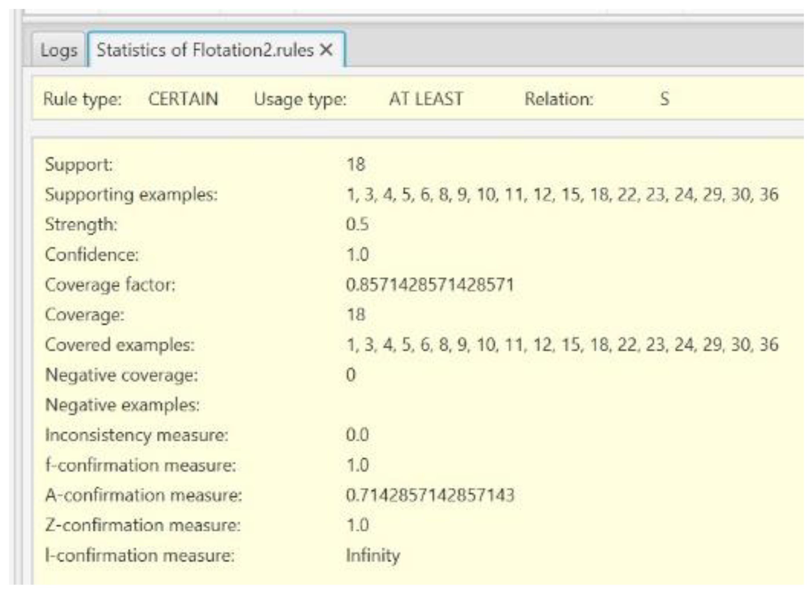
Figure 2.
Graph of model preferences.
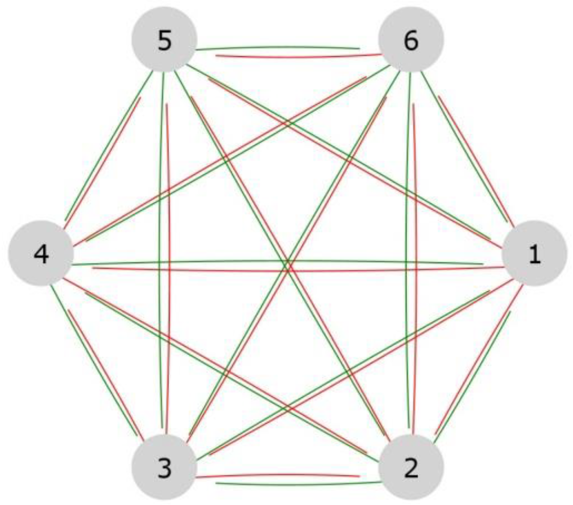
Table 1.
Important criteria dictating reagent selection and trade-off [4].
Table 1.
Important criteria dictating reagent selection and trade-off [4].
| Technical factors | Constraints |
|---|---|
| Reagent chemistry | Reagent regulatory approvals |
| Ore types, mineralogy and mineral chemistry | Handling |
| Frothing characteristics | Logistics |
| Water chemistry and gangue minerals | Toxicity and environmental issues |
| Stability | Odor |
| Particle size distribution | Manufacture |
| Downstream effects | Cost |
| Co-value minerals recovery | Strategic fit |
| Plant circuit, process conditions | |
| Plant constraints | |
| Compatibility with other reagents |
Table 2.
Contents of selected components in the ore [33].
Table 2.
Contents of selected components in the ore [33].
| Component | Contents |
|---|---|
| Cu | 0.270% |
| Cuox | 0.016% |
| S | 2.220% |
| Fe | 4.610% |
| Au | 0.190 g/t |
| Ag | 1.120 g/t |
Table 3.
Collector types used.
| Flotation collector | Collector type |
|---|---|
| FC1 | Potassium ethyl xanthate |
| FC2 | Sodium mercaptobenzothiazole + Sodium dithiophosphate (50% + 50%) |
| FC3 | Sodium dithiophosphate |
| FC4 | Sodium dialkyl dithiophosphinate |
| FC5 | Mixture of Isopropyl ethyl dithiophosphate and Sodium diisobutyl carbamate |
| FC6 | Ethoxycarbonyl isopropyl thiourea |
Table 10.
Pairwise comparisons (x outranks y (S), x does not outrank y (Sc)).
| Pair | Δq1 | Δq2 | Δq3 | Δq4 | Δq5 | Δq6 | Δq7 | Relation |
|---|---|---|---|---|---|---|---|---|
| {5, 5} | 0 | 0 | 0 | 0 | 0 | 0 | 0 | S |
| {5, 6} | 0.024 | -0.095 | 0.761 | -0.008 | -2.000 | -1160.000 | 5.774 | S |
| {5, 2} | 2.917 | -1.025 | 11.491 | -0.061 | 2.000 | -4260.000 | -0.416 | S |
| {5, 4} | 0.160 | -0.145 | 12.931 | 0.069 | -2.000 | 190.000 | -23.360 | S |
| {5, 3} | 0.147 | 0.263 | 5.191 | 0.009 | 2.560 | -2690.000 | -27.010 | S |
| {5, 1} | 4.554 | -0.442 | 13.069 | 0.070 | 3.000 | 2740.000 | -28.793 | S |
| {6, 5} | -0.024 | 0.095 | -0.761 | 0.008 | 2.000 | 1160.000 | -5.774 | Sc |
| {6, 6} | 0 | 0 | 0 | 0 | 0 | 0 | 0 | S |
| {6, 2} | 2.893 | -0.930 | 10.730 | -0.053 | 4.000 | -3100.000 | -6.190 | S |
| {6, 4} | 0.136 | -0.050 | 12.170 | 0.077 | 0.000 | 1350.000 | -29.134 | S |
| {6, 3} | 0.123 | 0.358 | 4.430 | 0.017 | 4.560 | -1530.000 | -32.784 | S |
| {6, 1} | 4.530 | -0.347 | 12.308 | 0.078 | 5.000 | 3900.000 | -34.567 | S |
| {2, 5} | -2.917 | 1.025 | -11.491 | 0.061 | -2.000 | 4260.000 | 0.416 | Sc |
| {2, 6} | -2.893 | 0.930 | -10.730 | 0.053 | -4.000 | 3100.000 | 6.190 | Sc |
| {2, 2} | 0 | 0 | 0 | 0 | 0 | 0 | 0 | S |
| {2, 4} | -2.757 | 0.880 | 1.440 | 0.130 | -4.000 | 4450.000 | -22.944 | S |
| {2, 3} | -2.770 | 1.288 | -6.300 | 0.070 | 0.560 | 1570.000 | -26.594 | S |
| {2, 1} | 1.637 | 0.583 | 1.578 | 0.131 | 1.000 | 7000.000 | -28.377 | S |
| {4, 5} | -0.160 | 0.145 | -12.931 | -0.069 | 2.000 | -190.000 | 23.360 | Sc |
| {4, 6} | -0.136 | 0.050 | -12.170 | -0.077 | 0.000 | -1350.000 | 29.134 | Sc |
| {4, 2} | 2.757 | -0.880 | -1.440 | -0.130 | 4.000 | -4450.000 | 22.944 | Sc |
| {4, 4} | 0 | 0 | 0 | 0 | 0 | 0 | 0 | S |
| {4, 3} | -0.013 | 0.408 | -7.740 | -0.060 | 4.560 | -2880.000 | -3.650 | S |
| {4, 1} | 4.394 | -0.297 | 0.138 | 0.001 | 5.000 | 2550.000 | -5.433 | S |
| {3, 5} | -0.147 | -0.263 | -5.191 | -0.009 | -2.560 | 2690.000 | 27.010 | Sc |
| {3, 6} | -0.123 | -0.358 | -4.430 | -0.017 | -4.560 | 1530.000 | 32.784 | Sc |
| {3, 2} | 2.770 | -1.288 | 6.300 | -0.070 | -0.560 | -1570.000 | 26.594 | Sc |
| {3, 4} | 0.013 | -0.408 | 7.740 | 0.060 | -4.560 | 2880.000 | 3.650 | Sc |
| {3, 3} | 0 | 0 | 0 | 0 | 0 | 0 | 0 | S |
| {3, 1} | 4.407 | -0.705 | 7.878 | 0.061 | 0.440 | 5430.000 | -1.783 | S |
| {1, 5} | -4.554 | 0.442 | -13.069 | -0.070 | -3.000 | -2740.000 | 28.793 | Sc |
| {1, 6} | -4.530 | 0.347 | -12.308 | -0.078 | -5.000 | -3900.000 | 34.567 | Sc |
| {1, 2} | -1.637 | -0.583 | -1.578 | -0.131 | -1.000 | -7000.000 | 28.377 | Sc |
| {1, 4} | -4.394 | 0.297 | -0.138 | -0.001 | -5.000 | -2550.000 | 5.433 | Sc |
| {1, 3} | -4.407 | 0.705 | -7.878 | -0.061 | -0.440 | -5430.000 | 1.783 | Sc |
| {1, 1} | 0 | 0 | 0 | 0 | 0 | 0 | 0 | S |
Table 11.
Induced rules.
| ID | Decision | <= | Condition 1 | Condition 2 | |
|---|---|---|---|---|---|
| 1 | x S y | <= | (diff_A7 <= -6.19) | ||
| 2 | x S y | <= | (diff_A1 >= -0.013) | & | (diff_A7 <= 0.0) |
| 3 | x S y | <= | (diff_A1 >= 0.024) | & | (diff_A7 <= 5.774) |
| 4 | x Sc y | <= | (diff_A7 >= 6.19) | ||
| 5 | x Sc y | <= | (diff_A1 <= 0.013) | & | (diff_A7 >= 3.65) |
| 6 | x Sc y | <= | (diff_A1 <= -0.024) | & | (diff_A7 >= -5.774) |
Table 12.
Final scores and collector ranking according to the DRSA.
| Collector | Overall flow score | Rank |
|---|---|---|
| FC1 | -10.0 | 6 |
| FC2 | 2.0 | 3 |
| FC3 | -6.0 | 5 |
| FC4 | -2.0 | 4 |
| FC5 | 10.0 | 1 |
| FC6 | 6.0 | 2 |
Table 13.
The normalized matrix.
| Flotation collector | A1 | A2 | A3 | A4 | A5 | A6 | A7 |
|---|---|---|---|---|---|---|---|
| FC1 | 0.0000 | 0.5474 | 0.0000 | 0.0000 | 1.0000 | 0.0000 | 0.0000 |
| FC2 | 0.3595 | 1.0000 | 0.1207 | 1.0000 | 0.8000 | 1.0000 | 0.8209 |
| FC3 | 0.9677 | 0.0000 | 0.6028 | 0.4656 | 0.9120 | 0.7757 | 0.0516 |
| FC4 | 0.9649 | 0.3168 | 0.0106 | 0.0076 | 0.0000 | 0.3643 | 0.1572 |
| FC5 | 1.0000 | 0.2042 | 1.0000 | 0.5344 | 0.4000 | 0.3914 | 0.8330 |
| FC6 | 0.9947 | 0.2780 | 0.9418 | 0.5954 | 0.0000 | 0.5571 | 1.0000 |
Table 14.
Fuzzified normalized matrix (L2 = H1 = 0.5).
| A1 | A2 | A3 | A4 | A5 | A6 | A7 | |||||||||||||||
|---|---|---|---|---|---|---|---|---|---|---|---|---|---|---|---|---|---|---|---|---|---|
| L | M | H | L | M | H | L | M | H | L | M | H | L | M | H | L | M | H | L | M | H | |
| FC1 | 1.00 | 0.00 | 0.00 | 0.00 | 0.91 | 0.09 | 1.00 | 0.00 | 0.00 | 1.00 | 0.00 | 0.00 | 0.00 | 0.00 | 1.00 | 1.00 | 0.00 | 0.00 | 1.00 | 0.00 | 0.00 |
| FC2 | 0.28 | 0.72 | 0.00 | 0.00 | 0.00 | 1.00 | 0.76 | 0.24 | 0.00 | 0.00 | 0.00 | 1.00 | 0.00 | 0.40 | 0.60 | 0.00 | 0.00 | 1.00 | 0.00 | 0.36 | 0.64 |
| FC3 | 0.00 | 0.06 | 0.94 | 1.00 | 0.00 | 0.00 | 0.00 | 0.79 | 0.21 | 0.07 | 0.93 | 0.00 | 0.00 | 0.18 | 0.82 | 0.00 | 0.45 | 0.55 | 0.90 | 0.10 | 0.00 |
| FC4 | 0.00 | 0.07 | 0.93 | 0.37 | 0.63 | 0.00 | 0.98 | 0.02 | 0.00 | 0.98 | 0.02 | 0.00 | 1.00 | 0.00 | 0.00 | 0.27 | 0.73 | 0.00 | 0.69 | 0.31 | 0.00 |
| FC5 | 0.00 | 0.00 | 1.00 | 0.59 | 0.41 | 0.00 | 0.00 | 0.00 | 1.00 | 0.00 | 0.93 | 0.07 | 0.20 | 0.80 | 0.00 | 0.22 | 0.78 | 0.00 | 0.00 | 0.33 | 0.67 |
| FC6 | 0.00 | 0.01 | 0.99 | 0.44 | 0.56 | 0.00 | 0.00 | 0.12 | 0.88 | 0.00 | 0.81 | 0.19 | 1.00 | 0.00 | 0.00 | 0.00 | 0.89 | 0.11 | 0.00 | 0.00 | 1.00 |
Table 15.
Final score and rank for the fuzzy-rough hybrid method.
| Flotation collector | Lower | Upper | Score | Rank |
|---|---|---|---|---|
| FC1 | 0.0000 | 0.0925 | 0.0463 | 6 |
| FC2 | 0.6000 | 0.6000 | 0.6000 | 3 |
| FC3 | 0.2000 | 0.5696 | 0.3848 | 5 |
| FC4 | 0.4000 | 0.5399 | 0.4699 | 4 |
| FC5 | 0.6304 | 1.0000 | 0.8152 | 1 |
| FC6 | 0.6700 | 0.8367 | 0.7534 | 2 |
Table 16.
Scores and approximation accuracies for four different FTN settings of the fuzzy-rough approach.
Table 16.
Scores and approximation accuracies for four different FTN settings of the fuzzy-rough approach.
| Flotation collector | 1st test | 2nd test | 3rd test | 4th test |
|---|---|---|---|---|
| FC1 | 0.0463 | 0.0681 | 0.0516 | 0.0570 |
| FC2 | 0.6000 | 0.6000 | 0.6000 | 0.6000 |
| FC3 | 0.3848 | 0.3547 | 0.3666 | 0.3970 |
| FC4 | 0.4699 | 0.4661 | 0.4624 | 0.4804 |
| FC5 | 0.8152 | 0.8453 | 0.8334 | 0.8030 |
| FC6 | 0.7534 | 0.7729 | 0.7660 | 0.7449 |
| Accuracy | 0.6872 | 0.7369 | 0.7184 | 0.6537 |
Table 21.
The ideal solution.
| A1 | A2 | A3 | A4 | A5 | A6 | A7 | |
|---|---|---|---|---|---|---|---|
| FCi | 96.901 | 3.837 | 35.450 | 0.586 | 2.000 | 7800.000 | 54.469 |
Table 22.
The normalized matrix of difference coefficients.
| FCi | A1 | A2 | A3 | A4 | A5 | A6 | A7 |
|---|---|---|---|---|---|---|---|
| FC1 | [0.883 1.000] | [0.402 0.485] | [0.985 1.000] | [0.867 0.982] | [0.000 0.000] | [1.000 1.000] | [0.936 1.000] |
| FC2 | [0.500 0.737] | [0.000 0.179] | [0.869 0.879] | [0.000 0.208] | [0.200 0.200] | [0.000 0.000] | [0.063 0.394] |
| FC3 | [0.004 0.140] | [0.763 1.000] | [0.389 0.404] | [0.436 0.634] | [0.088 0.088] | [0.224 0.224] | [0.894 0.947] |
| FC4 | [0.000 0.164] | [0.506 0.734] | [0.977 0.989] | [0.837 1.000] | [1.000 1.000] | [0.636 0.636] | [0.791 0.858] |
| FC5 | [0.009 0.085] | [0.677 0.755] | [0.000 0.007] | [0.460 0.505] | [0.600 0.600] | [0.609 0.609] | [0.121 0.326] |
| FC6 | [0.009 0.093] | [0.637 0.679] | [0.059 0.063] | [0.404 0.452] | [1.000 1.000] | [0.443 0.443] | [0.000 0.146] |
Table 23.
Final score and rank for the rough-grey method based on weights defined by the DM.
| DI lower | DI upper | Midpoint | Width | Rank | |
|---|---|---|---|---|---|
| FC1 | 0.770 | 0.845 | 0.808 | 0.075 | 6 |
| FC2 | 0.300 | 0.478 | 0.389 | 0.179 | 3 |
| FC3 | 0.405 | 0.524 | 0.465 | 0.118 | 4 |
| FC4 | 0.532 | 0.655 | 0.593 | 0.123 | 5 |
| FC5 | 0.263 | 0.337 | 0.300 | 0.074 | 2 |
| FC6 | 0.252 | 0.313 | 0.282 | 0.061 | 1 |
Table 24.
Net flows and ranking by the PROMETHEE method.
| Flotation collector | Ф+ | Ф- | Ф | Rank |
|---|---|---|---|---|
| FC1 | 0.2100 | 0.7900 | -0.5800 | 6 |
| FC2 | 0.5900 | 0.4100 | 0.1800 | 3 |
| FC3 | 0.4200 | 0.5800 | -0.1600 | 4 |
| FC4 | 0.3600 | 0.6300 | -0.2700 | 5 |
| FC5 | 0.7100 | 0.2900 | 0.4200 | 1 |
| FC6 | 0.7000 | 0.2900 | 0.4100 | 2 |
Table 25.
ELECTRE method ranking.
| Net outranking count | Not outranked1 | Rank | |
|---|---|---|---|
| FC1 | -2 | - | 5 |
| FC2 | +2 | + | 2 |
| FC3 | -1 | - | 4 |
| FC4 | -4 | - | 6 |
| FC5 | +3 | + | 1 |
| FC6 | +2 | + | 2 |
1Collectors marked with “+” are not outranked by any collector.
Table 26.
Final scores and rankings of methods used for flotation collector selection.
| DRSA | Rough-Fuzzy | Rough-Grey | PROMETHEE | ELECTRE | ||||||
|---|---|---|---|---|---|---|---|---|---|---|
| Score | Rank | Score | Rank | Score | Rank1 | Score | Rank | Net outranking count | Rank | |
| FC1 | -10 | 6 | 0.0463 | 6 | 0.808 | 6 | -0.5800 | 6 | -2 | 5 |
| FC2 | 2 | 3 | 0.6000 | 3 | 0.389 | 3 | 0.1800 | 3 | +2 | 2 |
| FC3 | -6 | 5 | 0.3848 | 5 | 0.465 | 4 | -0.1600 | 4 | -1 | 4 |
| FC4 | -2 | 4 | 0.4699 | 4 | 0.593 | 5 | -0.2700 | 5 | -4 | 6 |
| FC5 | 10 | 1 | 0.8152 | 1 | 0.300 | 2 | 0.4200 | 1 | +3 | 1 |
| FC6 | 6 | 2 | 0.7534 | 2 | 0.282 | 1 | 0.4100 | 2 | +2 | 2 |
1 The rough-grey results are based on DI midpoint (smaller is better).
Disclaimer/Publisher’s Note: The statements, opinions and data contained in all publications are solely those of the individual author(s) and contributor(s) and not of MDPI and/or the editor(s). MDPI and/or the editor(s) disclaim responsibility for any injury to people or property resulting from any ideas, methods, instructions or products referred to in the content. |
© 2026 by the authors. Licensee MDPI, Basel, Switzerland. This article is an open access article distributed under the terms and conditions of the Creative Commons Attribution (CC BY) license (http://creativecommons.org/licenses/by/4.0/).
Copyright: This open access article is published under a Creative Commons CC BY 4.0 license, which permit the free download, distribution, and reuse, provided that the author and preprint are cited in any reuse.