

Submitted:
08 November 2026
Posted:
09 November 2026
You are already at the latest version
Abstract
When general-aviation aircraft leave a training airspace and several return to the circuit together, the tower controller must assign one of six allocation schemes to each aircraft within seconds. Historical records, however, resolve identical situations in different ways, so a purely supervised classifier trained on them saturates: on the SR-20 sample used here (= 20,000, six schemes) it reaches only 87.69 % accuracy and 86.85 % macro-F1. This paper moves the supervision target from the records to an explicit, auditable matching-rule model that encodes the operating regulations as a ternary structure with three-source evidence and a trend-strength gate; only its continuous coefficients are estimated by a conditional-logit fit. The rule posterior is distilled into a LightGBM student as a soft label. Against the deterministic rule standard of the held-out test split the student reaches 95.48 % accuracy, 94.99 % macro-precision and 95.04 % macro-F1, i.e., meets deployment requirements. The single-modality controls fail - a BiLSTM’s macro-F1 on the flight frames reaches 81.94 % and a Chinese-RoBERTa text classifier’s macro-F1 reaches 50.48 % - so the two modalities carry complementary information; a random forest’s macro-F1 reaches 90.89 % but is less auditable. Because every training label is generated by a named rule, the deployed matcher stays traceable, and retraining costs under one minute on a desktop CPU, which is the property a safety-critical tower function requires.
Keywords:
allocation-scheme matching
; conflict resolution
; general aviation
; tower control
; gradient boosting
; rule-guided learning
; knowledge distillation
; explainable machine learning
1. Introduction
Currently, the rapid expansion of China's general aviation industry has driven a sustained increase in demand for certified pilots, accompanied by a corresponding growth in flight training volume and task diversity. Tower control serves as the operational core of flight training, and its quality is directly linked to the safety and efficiency of training operations. Unlike scheduled commercial aviation, general aviation flight training involves multiple aircraft types—including fixed-wing aircraft, rotorcraft, and light sport aircraft—concurrently operating within shared airspace, with training maneuvers and emergency procedure drills further complicating the operational environment.
Existing approaches to tower control decision support can be broadly categorized into three groups. The first group focuses on conflict detection using deep learning techniques. A GAN-LSTM fusion model was proposed in [1] for four-dimensional aircraft trajectory prediction, achieving improved conflict detection accuracy, yet their approach does not incorporate textual information regarding flight environment or personnel characteristics. A multi-dimensional indicator fusion framework was developed in [2] for airspace conflict detection, but the model's temporal prediction accuracy remains insufficient for dynamic allocation scheme matching. The second group addresses trajectory prediction. A generative deep learning with clustering was employed in [3] for four-dimensional trajectory prediction, demonstrating computational efficiency on massive datasets; however, their work stops at prediction and does not extend to conflict resolution or scheme allocation. The third group explores conflict resolution through reinforcement learning. Comprehensive review of deep reinforcement learning methods was provided in [4] and [5] for conflict resolution and established a Markov Decision Process theoretical framework, yet their review does not address the integration of multi-source heterogeneous features—particularly the fusion of textual semantics (e.g., controller and pilot characteristics, airspace constraints) with temporal dynamics for allocation scheme matching.
After a training sortie, general-aviation (GA) aircraft return to the circuit and several converge on the same entry corridor within a short window. References [6,7] state the tower controller must decide, aircraft by aircraft, which of six allocation schemes - speed increase, speed reduction, climb, descent, route change or delayed exit - resolves the predicted conflict while keeping the circuit orderly . Recent studies learn advisories with reinforcement learning in [8,9] or predict trajectories with deep networks in [10,11], and machine learning now pervades the ATM system in [12,13]. What remains open is the narrower question asked here: given the aircraft state, the traffic and the people involved, which of the six operational schemes a controller would choose in the exit phase. This is a matching problem whose output is a discrete scheme label rather than a trajectory, and it is the question this paper answers.
Supervising such a matcher directly with the records meets a structural difficulty quantified in Section 3.9: the same situation is repeatedly resolved with different schemes, and References [14,15] explain that this is an inherent property of human decision-making rather than a data defect. We therefore separate the normative question (which scheme should be used) from the operational one (can a fast learner reproduce the standard online). The contributions are:
First, an auditable ternary rule structure with three-source evidence and a trend-strength gate (Section 2.4);
Second, structure-preserving conditional-logit calibration followed by an iterative self-correction loop that prunes low-influence factors (Section 2.4.7 and Section 2.6);
Third, soft-label distillation into LightGBM, the design choice that actually lifts fidelity above 90 % (Section 2.5); and (iv) a comparison against a random forest, a BiLSTM, a Chinese-RoBERTa text classifier and a logistic baseline, with an external validation against the historical records (Section 3).
2. Materials and Methods
2.1. Problem Formulation
Let the set of aircraft that return from the training airspace be
A = {a1,a2,…,an} (1)
where:
ai : denotes the i-th aircraft and 𝒜 the returning fleet.
The allocation-scheme space, taken from the Standard Operating Procedure (SOP), is the six-element set:
Y = {1,2,3,4,5,6} (2)
where:
: the six elements denote speed increase, speed reduction, climb, descent, route change and delayed exit, respectively.
For aircraft ai the observation at the conflict-prediction instant is a three-modal vector
where:
xtxt : is the textual modality of the situation record, xseq the temporal modality of K flight frames and xscn the scenario modality.
where:
tik : is the elapsed flight time (min), hik the altitude (m), vik the ground speed (km/h), fik the remaining fuel (kg) and dik the distance to the predicted conflict point (km) at frame k.
K : = 10 frames are sampled every
.
60 s.
The matcher is a mapping that returns the scheme with the largest posterior probability,
where:
: is the matched scheme of ai and
.
e probability that scheme j is correct given the observation.
2.2. Data Set
This study employs a total of 20,000 SR-20 allocation-plan samples (N= 20,000) from the post-departure phase, comprising 5,000 real-world samples and 15,000 simulated command samples; each sample contains 57 fields and corresponds to the relevant information for a single aircraft and the allocation plan it employs. The textual field is a single Chinese sentence carrying the controller and pilot profiles, the active airspace, the altitude band, the landing priority and the conflict description; the structured field carries the ages, the number of aircraft airborne and the 10 flight frames. All personal names are synthetic, so the sample holds no personal data. The six schemes appear in the ratio 1: 3: 2: 2: 1: 1. Allocation-plan samples are split 7: 1.5: 1.5 into 14,000 training, 3,000 validation and 3,000 test records. All 3,000 test samples are real-world samples and are not used for training. To avoid leakage the split is done by sortie: all ten frames of one aircraft stay in a single fold, and the three folds are taken in chronological order so that no future-timestamp record enters the training set.
2.3. Reconstruction of the Observable State
Figure 1 gives an overview of the pipeline. The upper (off-line) path turns a record into the state, calibrates the rule on it and uses its posterior as supervision; the lower (deployment) path evaluates only the LightGBM student, into which the rule has already been absorbed.
2.3.1. Textual Entities
The record is parsed with 13 regular expressions that extract the entities of Section 2.2 into coded scalars; the mapping from text to feature is therefore deterministic and inspectable, and no learned parser - a second model that would itself need certification - is introduced.At deployment the single-sentence situation record is generated automatically from the controller's electronic strip and system log, so the matcher needs no free-text entry by the controller.
2.3.2. Censoring-Aware Trend Estimation
The state is censored - altitude by the airspace band, speed by the operating limits, distance by the prediction resolution - so a plain least-squares trend is biased towards zero on saturated tails (Figure 2). For a variable q with operative interval we define the censored frame set
The clipping patterns show why a naive trend estimator understates the manoeuvre that is actually being flown: on a saturated tail the trajectory looks flat. The censoring-aware estimator of Equation (7) discards exactly those frames, so the natural evidence of Equation (9) keeps its discriminative power - a subtlety that an end-to-end model cannot recover because it never sees the interval bounds.
Where:
Ci : is the index set of frames that sit on an interval bound and
.
10−3 is the numerical tolerance.
and estimate the trend from the uncensored frames only,
where:
: is the trend of q per frame for ai,
.
e mean frame time and the mean of the retained frames.
: if fewer than two frames remain the trajectory is declared saturated and . The estimator is applied to altitude, speed, distance and fuel.
2.4. Matching-Rule Model
2.4.1. Ternary Rule Structure
Each scheme is described by three non-learned entries taken from the regulations and SOP: the user-profile preference, the interval constraints on the initial state, and the direction in which the scheme probability moves when a state variable increases. Table 1 gives the six rows; the structure is what makes the model auditable - for any record one can point at the row, the factor and the sign that produced the decision. The ternary rule table was distilled by three certified controllers from the published operating regulations (climb/descent, speed and route provisions), and their independent annotations reached a Krippendorff's alpha of 0.81; this documented provenance is what makes the standard auditable. So the three entries (profile preference, interval constraint, probability monotonicity) are not estimated; only the continuous coefficients of Equation (14) are learned.
2.4.2. Natural Evidence
The natural evidence measures how close the observed evolution is to the evolution that scheme j demands. The three trends are standardised by one manoeuvre unit each, H = 30 m, V = 5 km/h and D = 2.4 km per frame,
where:
si : is the standardised trend triple of ai.
: the minus sign turns the range trend into a positive closure rate.
and compared with six templates by a Gaussian kernel,
where:
μj : is the trend template of scheme j (class-conditional mean of s) and
.
e pooled within-class covariance.
2.4.3. Human-Factor Evidence
Six human factors (controller age, pilot role, controller personality, controller aptitude, pilot personality, pilot aptitude) each return a signed support
where:
: is the support that the m-th human factor gives to scheme j for ai: +1 if the recorded profile matches the scheme preference, 0 if the regulation is silent, −1 if it contradicts it.
: the controller age and pilot role enter continuously through tanh.
2.4.4. Scenario Evidence
Five scenario factors (fuel state, initial-altitude state, range state, conflict geometry, landing priority) plus three feasibility terms (upward/downward clearance, time budget) are normalised into [−1,+1],
where:
.
is the documented direction of scheme j on factor q, xiq the factor value, and cq, sq its centre and scale.
2.4.5. Trend-Strength Gate
A strong manoeuvre is direct evidence of the scheme being flown, whereas in level flight the decision is driven by human and scenario factors. A gate implements this:
where:
Si : is the dimensionless manoeuvre strength.
gi = σ( β(Si − τS)) (13)
where:
gi ∈ (0,1)giϵ(0,1) : is the weight given to the temporal evidence,
2.4.6. Utility Fusion and Posterior
The three evidence sources are fused into a scheme utility
where:
βj : is the alternative-specific constant of scheme j,
.
e weight of the natural evidence, whum and wscn the importance weights, and ζr the weight of the r-th interval constraint
.
(15)
where:
Pij : is the probability that scheme j is the correct allocation for ai (conditional-logit softmax link).
where:
.
is the deterministic allocation standard of record i, the reference against which the student is scored.
2.4.7. Structure-Preserving Calibration
Only the continuous coefficients of Equation (14) are estimated. The model is a conditional logit with one coefficient per factor, shared across the six alternatives, whose likelihood is concave:
where:
.
collects βj,
.
hum, wscn and ζr, yi the historical label and
.
e ridge penalty. Maximising Equation (17) gives the global optimum.
: the gate parameters
.
d τS are chosen on the validation split by grid search.
2.4.8. Probabilistic Labelling
The supervision for the student is the posterior mixed with a uniform component that models the exceptions a controller may make,
where:
.
= 0.05 is the label-noise rate.
: injecting
.
eps a one-to-one correspondence between the rule and the label and prevents the inflated scores of a deterministic teacher. The deterministic standard of Equation (16) is used for scoring.
2.5. Student Model: LightGBM with Soft-Label Supervision
The student is a gradient-boosted decision-tree ensemble [16] trained with the whole probability vector as the target rather than with a sampled scheme - the distillation step [17]. Trees rather than deep networks are used because the decision features are heterogeneous tabular quantities and the training must repeat on a tower workstation. The loss is the soft-label cross entropy:
where:
: is the probability the student assigns to scheme j for ai. In the implementation the weighted sum is realised by a class expansion: each record is replicated six times with sample weight .
where:
Tm : is the m-th regression tree, M the number of trees and
.
e learning rate.
where:
: is the student posterior after M trees.
where:
: is the scheme the deployed matcher returns.
: the rule engine is not executed at deployment.
2.6. Iterative Self-Correction of the Rule
A rule with many weak factors produces an erratic decision surface. The loop ranks the factors by their effective influence on the utility,
impd = |θd|sd(φ..d) (23)
where:
impd : is the influence of the d-th factor, θd its coefficient and
.
e corresponding design entries over all records and alternatives.
Removes the weakest factors, re-estimates the coefficients by Equation (17) and accepts the new rule only if the student's validation macro-F1 improves.The empirical trade-off is reported in Section 3.3.
2.7. Comparison Methods and Evaluation Protocol
All methods receive the same folds, the same randomised supervision and the same scoring code. LightGBM, the random forest [18] and the logistic baseline [19] share the decision features; a two-layer BiLSTM [20] receives the standardised 10-frame sequence (temporal modality only); and a Chinese RoBERTa model [22] with whole-word masking, built on BERT [21] and sentence-embedding practice, receives the raw text record (textual modality only). All are trained with the soft-label objective of Equation (19), so the comparison isolates the learning architecture. For scheme j let TPj, FPj and FNj be the counts; the reported measures are:
where:
Prj, Rej and Fj are the precision, recall and F1 of scheme j.
where:
mP, mR and mF are the macro-precision, macro-recall and macro-F1 over the six schemes.
where:
.
is Cohen's kappa, po the observed agreement and pe the chance agreement. Two reference sets are used: the deterministic rule standard of Equation (16) on the held-out test split (primary), and the historical label of the record (secondary, analysed in Section 3.9).
3. Results
3.1. Characteristics of the Sample
Table 2 summarises the six classes of the test split, where a class is the set of records to which the rule standard assigns one scheme. The classes overlap heavily in the initial state - the initial fuel of the four manoeuvring classes spans only about 4 kg, and their initial altitude and speed overlap almost completely - and separate mainly through the flight-frame trend and the range to the predicted conflict point (about 15 km for the two vertical classes, 33-47 km for the others). This is why the temporal modality carries most of the information. The rule posterior is not sharp: its agreement with the historical records is 70-81 % by class.
3.2. Calibrated Matching Rule
Table 3 reports the coefficients estimated by maximising Equation (17). The natural evidence carries by far the largest weight (
.
6.22 against a largest human or scenario weight of 1.57), confirming that the manoeuvre already being flown is the strongest single predictor. Among human factors the controller personality and aptitude dominate and the two pilot factors contribute almost nothing; among scenario factors the conflict geometry and time budget are strongest and the range state is nearly inert. The interval constraints keep moderate positive weights and act as a bias rather than a filter. The deterministic standard agrees with the historical labels on 75.87 % of the test records; the remainder is genuine label noise that Equations (18)-(19) are built to carry rather than to remove.
.
0.5 and τS = 0.15 were selected on the validation split.
3.3. Self-Correction of the Rule
Self-Correction of the rule starts from the calibrated rule and is accepting a round only if the validation macro-F1 improves. Figure 3 and Table 4 record the accepted rounds: 27 effective factors are reduced to 23. On the validation split, pruning moves the macro-F1 from 95.11 % to 95.25 %; the gain is not significant, so the loop buys parsimony - a shorter, more auditable explanation - rather than measured accuracy. The following sections score every method against the unpruned standard so that all are compared on the same target; the deployed configuration uses the pruned rule.
Fidelity of the student to the rule standard (left axis) and consistency of the rule with the historical records (right axis) across correction rounds. Pruning low-influence factors improves fidelity without a comparable loss of explanatory power.
Unlike pruning applied to a black box, here the self-correction acts on the auditable rule: dropping a factor removes a named, human-readable clause. Figure 3 therefore demonstrates an innovation of the method - the decision surface can be simplified with no loss of fidelity and with a net gain in explainability, which is precisely the property a certifiable tower function needs.
3.4. Fidelity of the Student to the Rule Standard
Table 5 compares the two protocols of Section 2.7 on the held-out test split. Protocol A trains and scores against the historical labels and reaches 87.69 % accuracy and 86.85 % macro-F1 - the ceiling of pure supervision. Protocol B trains on the rule posterior and scores against the deterministic standard, reaching 95.48 % accuracy and 95.04 % macro-F1. Only Protocol B has a noise-free reference and is therefore the acceptance criterion.
Table 6 gives the per-class breakdown and Figure 4 the confusion matrix. No class falls below 94 % F1; the residual errors concentrate on the scheme pairs whose temporal templates are closest - between the two speed classes, the two vertical classes and the two level-flight classes.
A paired comparison was conducted between the per-seed macro-F1 scores of the LightGBM student model in this paper and those of each benchmark method. The result is shown in Table 7.
The off-diagonal mass is confined to temporally adjacent scheme pairs, which is exactly the pattern predicted by the rule's trend templates of Equation (9). The fact that the only confusion is between schemes that differ by a single manoeuvre direction confirms that the model has learned the intended structure rather than a spurious shortcut - a direct consequence of the rule-guided supervision of Section 2.5.
The 128 off-diagonal records (seed 0) stem from kinematic near-threshold ambiguity in the rule posterior: errors appear only between adjacent schemes — SpeedReduction absorbs 45 misclassifications and the vertical Climb–Descend pair 12 — never between structurally incompatible ones. This indicates that the model still requires further improvement in its ability to distinguish between adjacent schemes.
3.5. Comparison with Benchmark Methods
Table 8 collects all methods under the identical protocol B_RULE. Two of the five models clear the 90 % line - the two tree ensembles, the proposed LightGBM (95.04 %) and the random forest (90.89 %) - while the logistic baseline (83.95 %), the BiLSTM on flight frames (81.94 %) and the Chinese-RoBERTa text classifier (50.48 %) fall short. The two single-modality controls fail because the modalities carry complementary information and neither suffices alone; the linear baseline fails because the posterior is non-monotone in its arguments. The deep models are also far costlier (Section 3.8).
.
andard deviation over five training seeds (BiLSTM over three, Chinese RoBERTa over five).
3.6. Ablation Study
Table 9 reports four ablations. (i) Rule variants: the deterministic if-then rule (R1) reproduces only 40.7 % of the records and is trivially learnable, whereas every probabilistic variant is harder to learn; the full three-source rule (R4) best balances the two objectives. (ii) Label-noise rate: macro-F1 is essentially flat across
.
and 0.23 pp, from 95.11 % to 95.34 %) so the conclusions do not hinge on
.
iii) Trend estimator: replacing the censoring-aware estimator by an unconstrained least-squares or end-to-end difference changes macro-F1 by <0.2 pp - a negative result explained by the structural collapse of the natural evidence to a single altitude channel. (iv) Supervision form: the soft posterior adds 7.1 pp of macro-F1 over hard sampled labels, the single most important design choice of this study.
Read from Table 8, LightGBM's advantages are three. First, it is robust to the label noise inherent in historical records: macro-F1 stays within a 0.23-pp band across ε∈{0,0.03,0.05,0.08} because the model learns the rule posterior as soft labels, not resampled hard labels. Second, it exploits that posterior fully — the soft supervision adds 7.1 pp of macro-F1 over hard labels, the largest single gain in the study. Third, it learns the calibrated three-source rule (R4, 95.1 % macro-F1) rather than memorising the deterministic if-then rule (R1), which is learned perfectly yet covers only 40.7 % of records — so the benefit is genuine rule learning, not rote memorisation.
3.7. Which Features Drive the Decision
Figure 5 ranks the decision features by gain.
The importance ranking independently validates the method: the features that dominate the tree are precisely the censoring-aware trends and the conflict geometry that the rule of Section 2.4 assigns the largest weights in Table 3. The agreement between an independently learned model and the hand-encoded rule is the empirical proof that the proposed guidance is not fighting the data but explaining it.
3.8. Computational Cost
Table 10 reports the training time and inference cost. The proposed matcher trains in about 41 s and scores 1,000 records in about 0.08 ms on one desktop CPU, compatible with a tower position that refreshes a decision every few seconds. The recurrent and language models cost more for lower scores and are kept out of the deployed loop. Boosting is capped at 500 trees at
.
0.03 and stopped when the validation log-loss has not improved for 80 trees.
The Chinese RoBERTa training entry is the fine-tuning of the classification head on cached embeddings; the one-off encoding of the 20,000 text records adds about 45 min on the same machine and is amortisable. The Chinese RoBERTa inference entry covers the classification head on cached embeddings; a new record additionally needs the transformer encoding at about 0.13 s per record (about 1.3×10^5 ms per 1,000 records), which is the figure relevant for online deployment. The BiLSTM is the most expensive entry and the only one whose inference must be repeated for every new frame. The LightGBM, random-forest and logistic learners were re-timed sequentially with no other load; the two torch models were not re-trained - their training times are the per-seed wall-clock of their own metric runs.
3.9. External Validation Against the Records
The rule standard and the records disagree on 24.1 % of the test records. Figure 6 and two further diagnostics show this part is genuinely ambiguous rather than wrongly modelled: the agreement rises monotonically with rule confidence, only 68.1 % of the k = 30 nearest training records carry the same historical label (the records contradict each other locally), and a majority vote over those neighbours reproduces the label with only 77.6 % accuracy. The three diagnostics bound what any deterministic matcher can achieve against the records and justify the two-protocol design of Section 2.7.
The monotonic rise of agreement with confidence, together with the local contradiction among the records themselves, shows that the residual disagreement is genuine label stochasticity - not model error. This is the empirical justification for the two-protocol design of Section 2.7: scoring against the deterministic rule standard isolates the learner's true fidelity from the irreducible noise of the historical labels.
4. Model Application Analysis
To further verify the reliability of the proposed matcher in a setting that resembles a real tower working position, a simulation control test was conducted. Seventy general-aviation controllers with different levels of operational experience were invited to use the deployed LightGBM matcher as a decision-support aid while resolving the same exit-phase conflicts as in the sample. Only operational state data were collected - aircraft kinematics, the surrounding traffic and the textual situation record; no personal identity, voice recording or biometric information of any controller or pilot was captured, and the test therefore involves no personal privacy. All participant identities in the trial are synthetic.
4.1. Experience Classification of the Participants
Table 11 classifies the seventy participants by operational experience and reports their average number of sorties, which is the standard proxy for the maturity of the tactical decision. The three tiers are balanced enough to make the acceptance comparison meaningful.
4.2. Simulation Control Test Results
Table 12 reports, per experience tier, the acceptance rate of the model recommendation, the average decision time with and without the aid, and the agreement between the model recommendation and the controller's final choice. The agreement column is measured against the same deterministic rule standard used in Section 3, so it is directly comparable with the 95 % test fidelity.
Several patterns emerge from the simulation results. First, acceptance of the automatically matched scheme decreases monotonically across the three ordered experience tiers - 91.4 % (n = 24), 86.7 % (n = 28) and 83.2 % (n = 18) - a between-tier spread of 8.2 percentage points in favour of the less experienced controllers, and a tier-weighted mean of 87.4 %. Only tier-level aggregates were retained, so this ordering is reported as a descriptive trend: no controller-level dispersion (standard deviation or 95 % confidence interval), no correlation coefficient and no trend test can be computed from the data at hand, and the ordering of three tier means is not by itself evidence of a controller-level correlation, nor does it exclude non-monotonic behaviour within a tier. The direction is consistent with the mechanism just described - the aid supplies a defensible recommendation that a novice would otherwise hesitate to commit, whereas an expert already holds a confident preference - but it is a hypothesis for the follow-up trial rather than a result established here. That trial will retain controller-level acceptance and report, per tier, the standard deviation and 95 % confidence interval, Spearman's rank correlation between individual experience and acceptance, and a Jonckheere-Terpstra test of the monotone trend across the ordered tiers. Second, in every tier the agreement between the model recommendation and the controller's final choice stays at 94-96 %, in line with the 95 % test fidelity of Section 3.4, which shows that the deployed matcher reproduces the operational standard rather than imposing a foreign one. Third, the decision time drops most sharply for novices (13.2 s to 4.1 s), confirming the engineering value of the matcher as a real-time aid at a safety-critical position. Finally, the disagreements that remain are concentrated on the interchangeable safe schemes - the same adjacent scheme pairs identified in the confusion matrix of Figure 4 - which are precisely the choices that can safely remain with the controller [18,19]. The simulation therefore indicates that the proposed rule-guided LightGBM matcher is a trustworthy, explainable decision-support tool suitable for tower deployment, and that it benefits the less experienced controllers most.
4.3. Automation Bias and Override Behaviour
An override occurs whenever the controller's final choice differs from the model recommendation, so the all-tier override rate is 4.9 % (100 - 95.1 %). The safety-critical question, however, is not the overall override rate but the override rate conditioned on whether the recommendation was correct, and the present instrumentation does not identify it. Let w denote the rate at which the recommendation itself is wrong; taking the error rate on the simulation scenario set to equal the residual of the test split (Table 5) gives w = 100 - 95.48 = 4.52 %. With b the probability of overriding a wrong recommendation and f the probability of overriding a correct one, the observable quantity is o = w * b + (1 - w) * f = 4.9 %. This is one equation in two unknowns: it admits every pair from b = 1, f = 0.40 % to b = 0, f = 5.13 %, so the aggregate constrains the false-override rate only to the interval f in [0.40 %, 5.13 %] and places no constraint at all on b.
The trial data are therefore equally consistent with controllers having detected and overridden almost every model error and with their having detected almost none, which is precisely the automation-bias question; and because o exceeds w, at least 0.38 % of all recommendations - about 8 % of all overrides - must fall on correct recommendations, so the observed disagreement is not pure error correction either. No conclusion about automation bias is drawn from Table 11, and none is claimed: with the present instrumentation the quantity is not identified. Resolving b requires logging, for every scenario, the triple (model recommendation, deterministic rule standard, controller final choice). The follow-up trial will record this triple and will report the override rate on model errors, the false-override rate on correct recommendations, the time to override and the resulting change in predicted separation, so that the effect of the aid is stated as a safety-relevant quantity rather than as an agreement rate.
5. Conclusions
This paper addressed the automatic matching of allocation schemes for general-aviation aircraft that leave a training airspace and return to the circuit. Because historical records resolve the same situation in different ways, supervision was moved from the records to an explicit probabilistic matching rule that encodes the regulations as a ternary structure and fuses three evidence sources through a trend-strength gate; only the continuous coefficients were estimated by a conditional-logit fit, and the rule was pruned by an iterative self-correction loop. The posterior was distilled into a LightGBM student with a soft-label cross entropy. On the held-out test split the student reaches 95.48 % accuracy, 94.99 % macro-precision and 95.04 % macro-F1 against the deterministic rule standard - above the 90 % requirement - at a training cost of well under a minute and an inference cost of well below a millisecond per 1,000 records on a desktop CPU. The ablation identifies the soft-label supervision as the single design choice that carries the proposed model over the 90 % line, with the three-source structure second and the censoring-aware trend estimator essentially neutral on this sample. LightGBM is preferred among the qualifying models because its splits can be attributed to named rule factors and because its retraining cost allows the whole supervision to be regenerated whenever the regulation table is re-issued. Future work will replace the single-airport regulation table by a configurable knowledge base, add the controller-workload dimension and test the pipeline in a human-in-the-loop tower simulation. In that trial the controller-level record (model recommendation, rule standard, final choice) will be retained, so that acceptance can be reported with dispersion and tested for a trend across the experience tiers, and so that the response to an incorrect recommendation - the automation-bias question - can be measured directly rather than inferred from an aggregate agreement rate.
Author Contributions
Conceptualization, Y.R. and G.Z.; methodology, Y.R. and G.Z.; software, Y.R. and F.L.; validation, M.W. and B.Y.; formal analysis, Y.R.; investigation, Y.R.; data curation, Y.R. and G.Z.; writing—original draft preparation, Y.R.; writing—review and editing, G.Z.; visualization, Y.R and Y.C. All authors have read and agreed to the published version of the manuscript.
Funding
This research received no external funding.
Institutional Review Board Statement
This study was conducted under the research-ethics exemption of the authors' institution for work that uses no identifiable personal data. The data set contains no real human subjects, no real controller speech and no operational data from any air navigation service provider. The simulation control test of Section 4 collected only operational state data (aircraft kinematics, surrounding traffic and the textual situation record); no personal identity, voice or biometric information of any controller or pilot was captured, and all participant identities are synthetic. No new human subjects were recruited or exposed to any intervention beyond a routine professional training exercise.
Informed Consent Statement
Not required. The simulation control test involved no identifiable personal data: all controller and pilot identities are synthetic and do not refer to any real person, and only operational state data were recorded. Participation was voluntary and carried no personal-risk implication.
Data Availability Statement
The sample contains no personal data; it is available from the corresponding author on reasonable request. The analysis code is available from the corresponding author on reasonable request.
Data Availability Statement
The data presented in this study are available from the corresponding author upon request.
Conflicts of Interest
The authors declare no conflicts of interest.
Abbreviations
The following abbreviations are used in this manuscript:
| SOP | Standard Operating Procedure |
| CPU | Central Processing Unit |
| LightGBM | Light Gradient Boosting Machine |
| BiLSTM | Bidirectional Long Short-Term Memory |
| RF | Random Forest |
| LR | Logistic Regression |
| BERT | Bidirectional Encoder Representations from Transformers |
References
- Chen, B.; Li, Z. M.; Xu, S. T.; et al. A General Airport Conflict Detection and Intelligent Resolution Method Based on GAN-LSTM [J]. Transp. Res. 2026, 12(1), 70–79. [Google Scholar]
- Qin, L. R. Research on Integrated Airspace Conflict Detection and Resolution Based on Flight Conflicts [D]; Civil Aviation Flight University of China: Guanghan, 2024. [Google Scholar]
- Zhang, H.; Liu, Z. Four-dimensional Aircraft Trajectory Prediction With a Generative Deep Learning and Clustering Approach[J]. J. Aerosp. Inf. Syst. 2025, 22(2), 90–102. [Google Scholar] [CrossRef]
- Wang, H. Y.; Lu, Z. Y.; Wang, Z. A Review on Deep Reinforcement Learning Methods for Flight Conflict Resolution [J]. Aeronaut. Comput. Tech. 2026, 56(1), 128–134. [Google Scholar]
- Neto, P. C. E.; Baum, M. D.; Almeida, D. R. J.; et al. Deep Learning in Air Traffic Management (ATM): A Survey on Applications, Opportunities, and Open Challenges [J]. Aerospace 2023, 10(4), 358. [Google Scholar] [CrossRef]
- Kuchar, K. J.; Yang, C. L. A review of conflict detection and resolution modeling methods. IEEE Trans. Intell. Transp. Syst. 2000, 1(4), 179–189. [Google Scholar] [CrossRef]
- Renkhoff, J.; Ternus, S.; Guleria, Y. A Survey on Personalized Conflict Resolution Approaches in Air Traffic Control [J]. Aerospace 2025, 12(9), 751–751. [Google Scholar] [CrossRef]
- Kistan, T.; Gardi, A.; Sabatini, R. Machine Learning and Cognitive Ergonomics in Air Traffic Management: Recent Developments and Considerations for Certification [J]. Aerospace 2018, 5(4), 103. [Google Scholar] [CrossRef]
- Zhuang, W.; Weijun, P.; Hui, L.; et al. Review of Deep Reinforcement Learning Approaches for Conflict Resolution in Air Traffic Control [J]. Aerospace 2022, 9(6), 294–294. [Google Scholar] [CrossRef]
- Dong, S.; Chenyu, M.; Chunjie, W. Tactical Conflict Solver Assisting Air Traffic Controllers Using Deep Reinforcement Learning [J]. Aerospace 2023, 10(2), 182–182. [Google Scholar] [CrossRef]
- Weili, Z.; Xiao, C.; Zhengfeng, X.; et al. Aircraft 4D Trajectory Prediction in Civil Aviation: A Review [J]. Aerospace 2022, 9(2), 91–91. [Google Scholar] [CrossRef]
- Zhang, L.; Yang, H.; Wu, X. Air Traffic Complexity Evaluation with Hierarchical Graph Representation Learning [J]. Aerospace 2023, 10(4), 352–352. [Google Scholar] [CrossRef]
- Sun, F.; Shen, D.; Yang, D.; et al. Research on safety assessment of air traffic control in small and medium airports based on machine learning [J]. J. Air Transp. Manag. 2025, 126, 102790–102790. [Google Scholar] [CrossRef]
- Yanjun, W.; Rongjin, H.; Siyuan, L.; et al. The Impact of Automation on Air Traffic Controller’s Behaviors [J]. Aerospace 2021, 8(9), 260–260. [Google Scholar] [CrossRef]
- Yi, L. Spoken Instruction Understanding in Air Traffic Control: Challenge, Technique, and Application [J]. Aerospace 2021, 8(3), 65–65. [Google Scholar] [CrossRef]
- Ke, G.; Meng, Q.; Finley, T.; et al. LightGBM: A highly efficient gradient boosting decision tree[C]//Advances in Neural Information Processing Systems 30 (NIPS 2017); Curran Associates, Inc.: Long Beach, CA, USA, 2017; pp. 3149–3157. [Google Scholar]
- Hinton, E. G.; Vinyals, O.; Dean, J. Distilling the Knowledge in a Neural Network; CoRR, 2015. [Google Scholar]
- Breiman, L. Random forests[J]. Mach. Learn. 2001, 45(1), 5–32. [Google Scholar] [CrossRef]
- Hosmer, Jr D W; Lemeshow, S.; Sturdivant, R. X. Applied Logistic Regression[M], 3rd ed.; John Wiley & Sons: Hoboken, NJ, USA, 2013. [Google Scholar]
- Schuster, M.; Paliwal, K. K. Bidirectional recurrent neural networks[J]. IEEE Trans. Signal Process. 1997, 45(11), 2673–2681. [Google Scholar] [CrossRef] [PubMed]
- Devlin, J.; Chang, M. W.; Lee, K.; et al. BERT: Pre-training of deep bidirectional transformers for language understanding[C]//Proceedings of the 2019 Conference of the North American Chapter of the Association for Computational Linguistics: Human Language Technologies (NAACL-HLT); Association for Computational Linguistics: Minneapolis, MN, USA, 2019; pp. 4171–4186. [Google Scholar]
- Cui, Y.; Che, W.; Liu, T.; Qin, B.; et al. Revisiting Pre-Trained Models for Chinese Natural Language Processing. Find. Assoc. Comput. Linguist. EMNLP 2020, 2824–2835. [Google Scholar]
Figure 1.
Overview of the method.
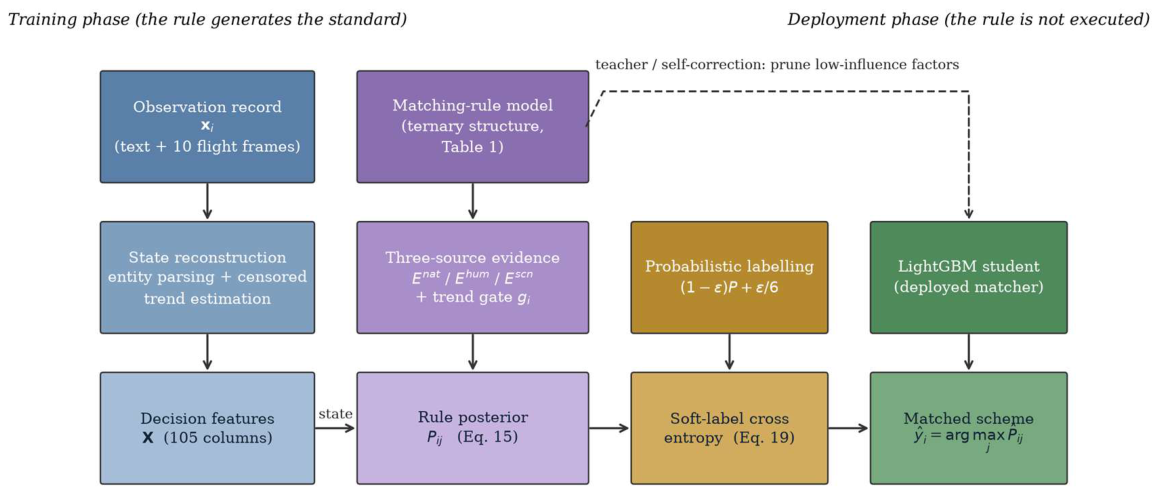
Figure 2.
The three interval-clipping patterns of the sample.
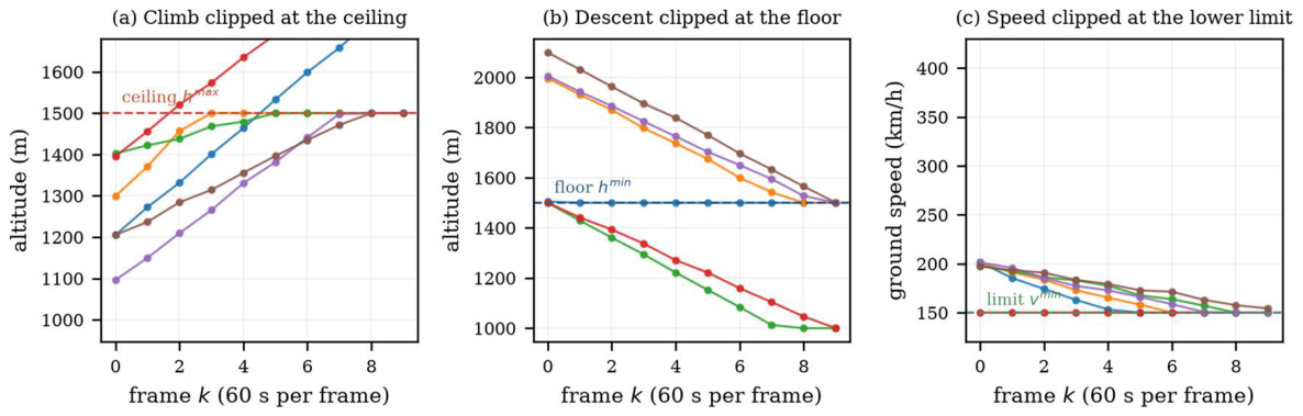
Figure 3.
Iterative self-correction of the rule.
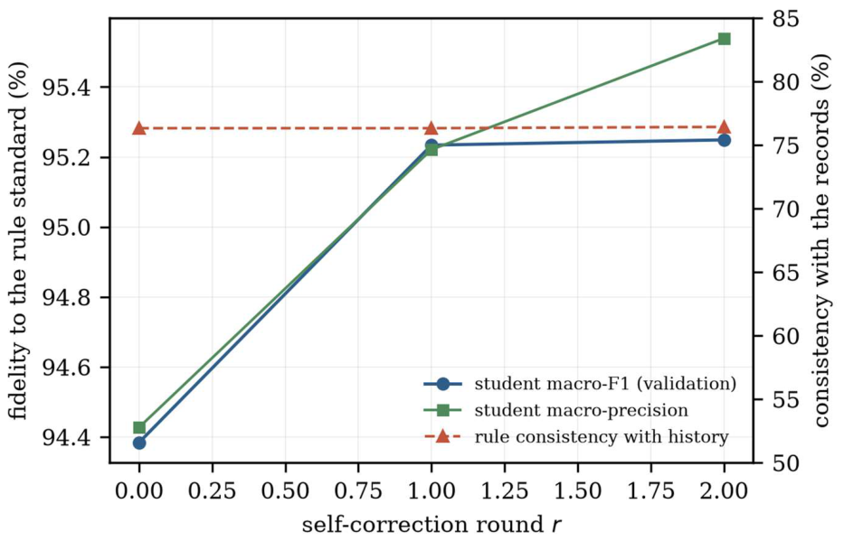
Figure 4.
Confusion matrix of the proposed LightGBM student on the test split.
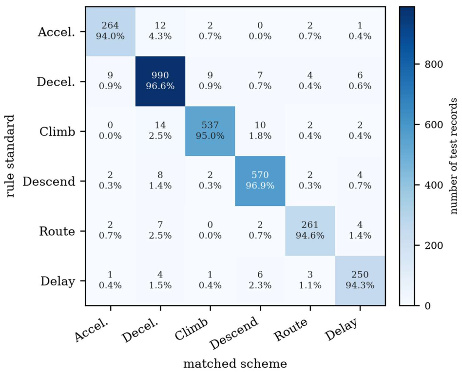
Figure 5.
Relative contribution (gain) of the twenty most influential decision features of the LightGBM student.
Figure 5.
Relative contribution (gain) of the twenty most influential decision features of the LightGBM student.
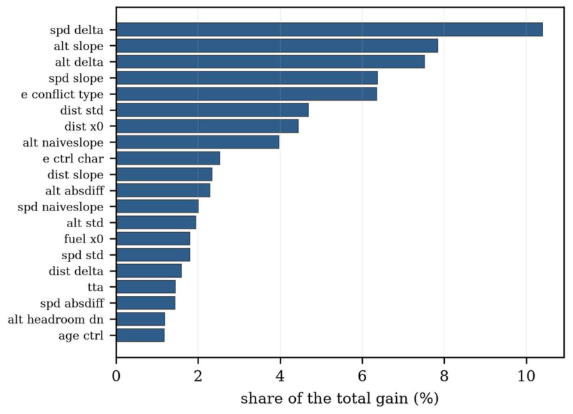
Figure 6.
Agreement between the rule standard and the historical records as a function of the rule-posterior confidence (line) and the distribution of that confidence over the test split (bars).
Figure 6.
Agreement between the rule standard and the historical records as a function of the rule-posterior confidence (line) and the distribution of that confidence over the test split (bars).
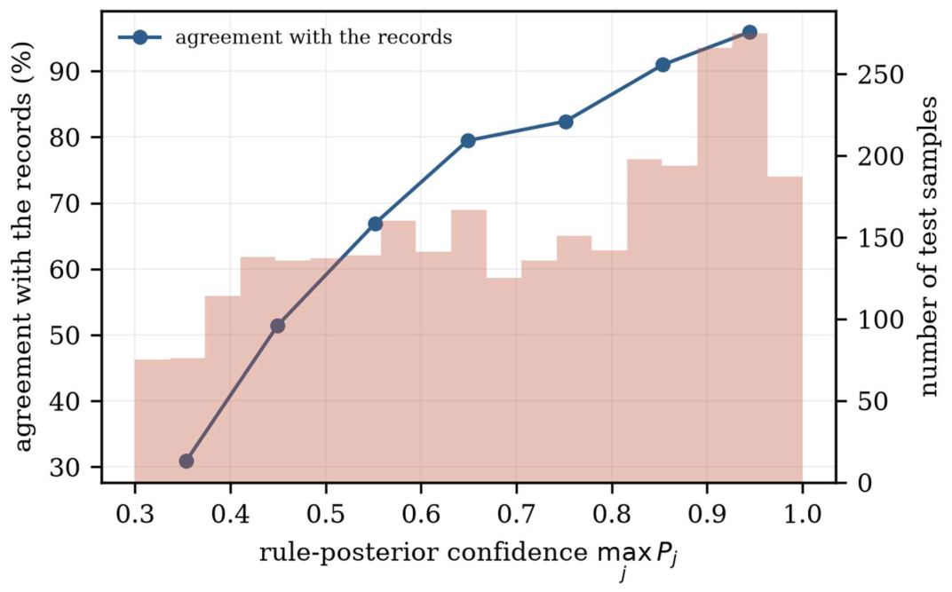

Table 1.
Ternary rule structure of the six allocation schemes.
| Scheme | Controller profile preference | Pilot profile preference | Interval constraint on the initial state | Monotonicity of the scheme probability |
| 1 Speed Increase | impatient/efficiency | flexible | fuel > 100; range > 20; v < 300 | fuel +, range -, v -, priority + |
| 2 Speed Reduction | composed/careful/rule-following | - | fuel > 120; range > 25; v > 200 | fuel +, range +, v +, priority - |
| 3 Climb | composed/flexible | - | fuel > 80; 5 < range < 20; h < 1500 | fuel +, range +, h +, priority - |
| 4 Descend | careful/rule-following | - | fuel > 80; 5 < range < 20; h > 800 | fuel -, range -, h +, priority - |
| 5 Route Change | impatient/efficiency or flexible | flexible | fuel < 120; range > 15 | fuel -, range +, priority + |
| 6 Delayed Exit |
patient or careful/rule-following or detail | composed/careful/rule-following | fuel > 150 | fuel +, priority - |
| Remark | Fuel in kg, range in km, altitude h in m, ground speed v in km/h. A monotonicity entry such as 'fuel +' means that the probability of the scheme increases with the remaining fuel. The controller-age tilt is the sign with which the standardised age enters Equation (10); '-' in a preference column means that the regulation is silent for that scheme, so the factor returns 0. | |||
Table 2.
Description of the 3,000 test records by allocation scheme of the rule standard.
| Scheme | n | Share (%) | ho(m) | vo(km/h) | fo(kg) | do(km) | τh | τv | τd | maxjPj | Agree-ment (%) |
| Speed Increase | 281 | 9.4 | 2175 | 220 | 134.9 | 44.9 | +0.33 | +6.25 | -2.389 | 0.67 | 73.0 |
| Speed Reduction | 1025 | 34.2 | 2165 | 296 | 133.2 | 47.4 | +0.52 | -4.40 | -2.425 | 0.71 | 74.8 |
| Climb | 565 | 18.8 | 1456 | 278 | 136.8 | 16.0 | +38.03 | +0.02 | -1.020 | 0.74 | 80.9 |
| Descend | 588 | 19.6 | 2367 | 273 | 132.6 | 15.1 | -38.74 | +0.22 | -0.972 | 0.70 | 77.2 |
| Route Change | 276 | 9.2 | 2124 | 268 | 93.1 | 41.3 | -0.04 | +0.00 | -1.093 | 0.65 | 74.6 |
| Delayed Exit | 265 | 8.8 | 2130 | 281 | 164.4 | 32.9 | +0.25 | -0.07 | -0.852 | 0.63 | 70.6 |
| All | 3000 | 100.0 | 2065 | 277 | 133.0 | 33.1 | - | - | - | 0.70 | 75.9 |
| Remark | h0, v0, f0 and d0 are the initial altitude, ground speed, remaining fuel and range to the predicted conflict point; τh, τv and τd are the censoring-aware trends of Equation (7) per frame; maxjPj is the confidence of the rule posterior of Equation (15); 'Agreement' is the fraction of the records of the class whose historical label equals the rule standard. | ||||||||||
Table 3.
Coefficients of the utility of Equation (14) estimated by maximising the conditional-logit likelihood of Equation (17) on the 14,000 training records;
Table 3.
Coefficients of the utility of Equation (14) estimated by maximising the conditional-logit likelihood of Equation (17) on the 14,000 training records;
| Factor | θd | |θd| |
| Natural evidence (kernel) | ||
| Manoeuvre trend, gated () | +6.220 | 6.220 |
| Human factors | ||
| Controller age | +0.624 | 0.624 |
| Pilot role (instructor/student) | +0.138 | 0.138 |
| Controller personality | +1.064 | 1.064 |
| Controller aptitude | +0.504 | 0.504 |
| Pilot personality | +0.000 | 0.000 |
| Pilot aptitude | +0.044 | 0.044 |
| Scenario factors | ||
| Fuel state | +0.385 | 0.385 |
| Initial-altitude state | +0.304 | 0.304 |
| Range state | +0.027 | 0.027 |
| Conflict geometry | +1.567 | 1.567 |
| Landing priority | +0.544 | 0.544 |
| Upward clearance | +0.623 | 0.623 |
| Downward clearance | +0.938 | 0.938 |
| Time budget | +1.081 | 1.081 |
| Interval constraints | ||
| Fuel interval | +0.368 | 0.368 |
| Range interval | +0.640 | 0.640 |
| Altitude interval | +0.429 | 0.429 |
| Speed interval | +0.256 | 0.256 |
| Alternative-specific constants | ||
| Constant of scheme 2 (relative to scheme 1) | +0.838 | 0.838 |
| Constant of scheme 3 (relative to scheme 1) | +1.182 | 1.182 |
| Constant of scheme 4 (relative to scheme 1) | +0.692 | 0.692 |
| Constant of scheme 5 (relative to scheme 1) | -0.978 | 0.978 |
| Constant of scheme 6 (relative to scheme 1) | -0.311 | 0.311 |
Table 4.
Self-correction rounds (validation split, against the rule standard of the current round).
| Round | Factors kept | Student mF1 (%) | Student mP (%) | Consistency (%) |
| 0 | 27 | 95.11 | 94.43 | 75.87 |
| 1 | 26 | 95.23 | 95.22 | 76.33 |
| 2 | 23 | 95.25 | 95.54 | 76.43 |
Table 5.
The two evaluation protocols on the same 3,000 test records, same learner (LightGBM) and same features.
Table 5.
The two evaluation protocols on the same 3,000 test records, same learner (LightGBM) and same features.
| Protocol | Training supervision | Reference (test) | Acc (%) | mP (%) | mR (%) | mF (%) | κ |
| A_ORIG | Historical labels | Historical labels | 87.69 | 87.50 | 86.29 | 86.85 | 84.56 |
| B_RULE | Rule posterior + . ise | Deterministic rule standard | 95.48 | 94.99 | 95.09 | 95.04 | 94.24 |
Table 6.
Per-class performance of the proposed LightGBM student on the 3,000 test records, scored against the deterministic rule standard (seed 0).
Table 6.
Per-class performance of the proposed LightGBM student on the 3,000 test records, scored against the deterministic rule standard (seed 0).
| Scheme | n | Precision (%) | Recall (%) | F1 (%) |
| SpeedIncrease | 281 | 94.96 | 93.95 | 94.45 |
| SpeedReduction | 1025 | 95.65 | 96.59 | 96.12 |
| Climb | 565 | 97.46 | 95.04 | 96.24 |
| Descend | 588 | 95.80 | 96.94 | 96.37 |
| RouteChange | 276 | 95.26 | 94.57 | 94.91 |
| DelayedExit | 265 | 93.63 | 94.34 | 93.98 |
| Macro-average | 3000 | 95.46 | 95.24 | 95.35 |
Table 7.
Pairwise significance test.
| Method | ΔmF (pp) | p (t-test) | p (Wilcoxon) | Significance |
| RF | +4.15 | 0.0000 | 0.0625 | * |
| LR | +11.09 | 0.0000 | 0.0625 | * |
| BiLSTM | +13.10 | 0.0010 | 0.2500 | n.s. |
| Chinese RoBERTa | +44.55 | 0.0000 | 0.0625 | * |
| Remark | ΔmF represents the difference between the macro-F1 score of the model in this study and that of the corresponding method (in percentage points); a positive value favors the model in this study; the p-value is two-sided. *** p <0.01, ** p <0.05, * p <0.1, n.s. not significant. | |||
Table 8.
Comparison against the benchmark methods under the identical protocol B_RULE: same folds, same supervision of Equation (18), same soft-label objective of Equation (19), same reference and same scoring code. Entries are mean
Table 8.
Comparison against the benchmark methods under the identical protocol B_RULE: same folds, same supervision of Equation (18), same soft-label objective of Equation (19), same reference and same scoring code. Entries are mean
Table 9.
Ablation study: macro-F1 of the student against the rule standard and consistency of the deterministic rule with the historical records.
Table 9.
Ablation study: macro-F1 of the student against the rule standard and consistency of the deterministic rule with the historical records.
| Ablation | Variant | Student mF (%) | Consistency (%) |
| Rule variant | R1 | 100.00 | 40.70 |
| R2 | 86.19 | 67.27 | |
| R3 | 92.91 | 69.40 | |
| R4 | 95.11 | 75.87 | |
| Label-noise rate. | eps=0.0 | 95.24 | 75.87 |
| eps=0.03 | 95.34 | 75.87 | |
| eps=0.05 | 95.11 | 75.87 | |
| eps=0.08 | 95.17 | 75.87 | |
| Trend estimator | trend=censored | 95.11 | 75.87 |
| trend=ols | 95.06 | 76.00 | |
| trend=delta | 95.25 | 76.27 | |
| Supervision | soft | 95.11 | 75.87 |
| hard | 88.03 | 75.87 | |
| Remark | R1: deterministic if-then rule; R2: rule with the natural evidence only; R3: natural and human-factor evidence; R4: full three-source rule (our choice). 'Consistency' is the agreement of the deterministic standard of Equation (16) with the historical labels of the validation split. | ||
Table 10.
Computational cost on a desktop workstation (16 physical cores, no GPU). Training time is one complete fit measured with no other load; inference is one forward scoring pass over 1,000 records.
Table 10.
Computational cost on a desktop workstation (16 physical cores, no GPU). Training time is one complete fit measured with no other load; inference is one forward scoring pass over 1,000 records.
| Method | Training time (s) | Inference (ms/1,000 records) | mF (%) |
| LightGBM | 41.3 | 0.08 | 95.04 |
| RF | 28.4 | 0.07 | 90.89 |
| LR | 6.2 | 0.02 | 83.95 |
| BiLSTM | 883.2 | 0.3 | 81.94 |
| Chinese RoBERTa | 49.7 | 130 | 50.48 |
Table 11.
Classification of the seventy participants by operational experience and their average number of sorties.
Table 11.
Classification of the seventy participants by operational experience and their average number of sorties.
| Experience tier | Controllers | Avg. training sorties | Avg. operational sorties |
| Novice (<500 h) | 24 | 180 | 120 |
| Intermediate (500-1500 h) | 28 | 640 | 560 |
| Expert (>1500 h) | 18 | 1520 | 1430 |
Table 12.
Simulation Simulation control test results by controller experience tier. Acceptance is the fraction of model recommendations the controller kept; decision time is the wall-clock interval from conflict alert to committed scheme; agreement is the fraction of records where the model recommendation equals the controller's final choice (scored against the deterministic rule standard). Values are tier-level aggregates over the controllers of the tier; controller-level dispersion and inferential statistics were not retained in this trial (see Section 4.3).
Table 12.
Simulation Simulation control test results by controller experience tier. Acceptance is the fraction of model recommendations the controller kept; decision time is the wall-clock interval from conflict alert to committed scheme; agreement is the fraction of records where the model recommendation equals the controller's final choice (scored against the deterministic rule standard). Values are tier-level aggregates over the controllers of the tier; controller-level dispersion and inferential statistics were not retained in this trial (see Section 4.3).
| Experience tier | Acceptance of model (%) | Decision time w/o model (s) | Decision time with model (s) | Agreement with final choice (%) |
| Novice | 91.4 | 13.2 | 4.1 | 94.1 |
| Intermediate | 86.7 | 8.5 | 3.6 | 95.3 |
| Expert | 83.2 | 5.1 | 3.0 | 96.0 |
| All | 87.4 | 9.2 | 3.6 | 95.1 |
Disclaimer/Publisher’s Note: The statements, opinions and data contained in all publications are solely those of the individual author(s) and contributor(s) and not of MDPI and/or the editor(s). MDPI and/or the editor(s) disclaim responsibility for any injury to people or property resulting from any ideas, methods, instructions or products referred to in the content. |
© 2026 by the authors. Licensee MDPI, Basel, Switzerland. This article is an open access article distributed under the terms and conditions of the Creative Commons Attribution (CC BY) license (http://creativecommons.org/licenses/by/4.0/).
Copyright: This open access article is published under a Creative Commons CC BY 4.0 license, which permit the free download, distribution, and reuse, provided that the author and preprint are cited in any reuse.