
Submitted:
03 November 2026
Posted:
05 November 2026
You are already at the latest version
Abstract
To reduce diagnostic uncertainty in hydraulic systems during vessel operation, this study investigated the correlation between fault features and monitoring parameters. Using monitoring data collected under normal operating conditions as the baseline, the association strength between multi-source monitoring features and ten fault modes was quantified via standardized deviation (Z-scores). On this basis, a hierarchical weight matrix, incorporating correlations between faults and features, devices and features, and subsystems and features, as well as lateral coupling coefficients, was constructed to capture hidden associations among signals, devices, and subsystems. Subsequently, a PGC-LightGBM algorithm was proposed, which embedded prior knowledge from the hierarchical weight matrix into model training through differentiated sample weighting: fault samples exhibiting larger deviations on physically correlated features were assigned higher training weights, thereby enabling multi-level fault diagnosis that accounts for multi-fault coupling and operational interactions across the entire hydraulic system. On a marine hydraulic pump station test bench dataset, the proposed method improved the macro-averaged F1 score from 75.3% to 77.8% under 5-fold stratified cross-validation, and from 63.2% to 68.2% on the independent test set. The fault-class average F1 rose from 59.9% to 65.4%, while the normal-class F1 of the weighted model reached 96.3%, remaining unaffected compared with 95.7% for the standard model. Ablation studies indicated that fault-level physically informed weights were the main contributing factor to the performance improvement, while device-level, subsystem-level, and lateral coupling components provided richer physical interpretability. This study provides an effective reference for reliability analysis and risk prediction in marine hydraulic systems.
Keywords:
hydraulic system
; fault diagnosis
; correlation analysis
; hierarchical weight matrix
; PGC-LightGBM
1. Introduction
Hydraulic transmission technology, owing to its high power density, rapid response, and precise controllability, has become an essential drive technology in modern ocean engineering, offshore engineering, and industrial automation. However, under non-steady-state operating conditions, the motion characteristics of hydraulic systems are complex and time-varying [1]; meanwhile, operating continuously under harsh conditions such as high temperature, high pressure, and heavy loads, these systems are prone to various faults, including hydraulic pump wear, valve spool sticking, oil leakage, and abnormal oil temperature. Owing to the inherent concealment of hydraulic faults, their pronounced nonlinear time-varying behavior, and the complex vibration transmission paths, fault diagnosis remains challenging [2]. Moreover, internal components are coupled through hydraulic circuits, and a fault in a single component can easily trigger cascading failures, rendering fault manifestations highly concealed and readily propagated [3]. Therefore, efficiently identifying multiple fault modes of hydraulic systems has become a key issue for ensuring safe equipment operation.
Existing studies on hydraulic fault diagnosis have established several technical approaches, mainly covering subjective judgment methods, signal-processing- and mathematical-model-based methods, and artificial-intelligence-based methods. Subjective judgment relies on the operator's sensory perception and experience; although simple to implement and inexpensive, its accuracy is limited, and it is applicable only to the qualitative diagnosis of simple equipment. Signal-processing-based methods achieve quantitative detection by analyzing oil, vibration, pressure, and flow signals. Zhu et al. [4] systematically reviewed fault diagnosis and health management technologies for hydraulic systems, pointing out that, due to the nonlinear time-varying behavior of hydraulic systems, feature extraction is challenging and establishing accurate mathematical models remains difficult. Rapur and Tiwari [5] combined on-line time-domain vibration and current signals with support vector machines to realize on-line multi-fault diagnosis of centrifugal pumps. Huang et al. [6] proposed the empirical mode decomposition method, providing an effective tool for the feature extraction of nonlinear and non-stationary signals. Yang et al. [7] applied fault tree analysis to the hydraulic system of a pipe bender; by establishing a logical fault structure, this technique enables early warning and rapid localization of common faults, but its construction is complex and heavily depends on expert experience.
With the development of artificial intelligence, intelligent diagnosis methods have become a research focus. Li et al. [8] applied a genetic-algorithm-optimized BP neural network to hydraulic fault diagnosis, achieving satisfactory results in fault identification by exploiting the nonlinear mapping and self-learning capabilities of neural networks. Wang et al. [9] applied support vector machines to the fault diagnosis of a hydraulically driven mechanical gear set; such models are suitable for small-sample nonlinear classification and can effectively distinguish different fault states by constructing an optimal separating hyperplane. Qiu et al. [10] summarized the application of deep learning methods, such as convolutional neural networks and long short-term memory networks, which can automatically extract features and process time-series signals, significantly improving diagnostic capability under complex operating conditions. Huang et al. employed a deep learning model based on multirate data samples, substantially improving the fault diagnosis accuracy of hydraulic systems [11]. Sun et al. utilized a convolutional neural network to identify time-frequency images of hydraulic pump vibration signals [12]. Dai et al. systematically reviewed signal-based intelligent hydraulic fault diagnosis methods and pointed out that the combination of signal processing and artificial intelligence is an important development direction [13].
In recent years, advanced technologies such as transfer learning, reinforcement learning, and digital twins have been increasingly applied to hydraulic fault diagnosis [10]. Transfer learning can alleviate the scarcity of labeled data and the limited cross-equipment applicability by transferring knowledge from a source domain to a target domain. Digital twins enable state synchronization between physical entities and virtual models, as well as predictive maintenance, by constructing virtual models, and can issue fault warnings in advance. Kosova and Unver [14] constructed a machine-learning-based digital twin framework for failure detection of aircraft hydraulic systems; the review of Qiu et al. [10] shows that digital twins can provide 7–21 days of early fault warning, effectively reducing maintenance risks and costs. Liang et al. proposed a hybrid digital twin model and successfully applied it to the fault diagnosis of hydraulic servo valves [15]. Shi et al. employed a two-stage multi-sensor information fusion strategy to effectively detect wear faults of hydraulic directional valves [16].
Although the studies above have achieved remarkable progress, there remains room for further improvement, particularly in algorithmic accuracy and interpretability. First, most existing methods—including the time-domain signal–SVM scheme of Rapur and Tiwari [5], the empirical mode decomposition of Huang et al. [6], the fault tree analysis of Yang et al. [7], and the SVM-based gear set diagnosis of Wang et al. [9]—treat each monitoring parameter as an independent feature and fail to exploit the multi-level association structure arising from the physical coupling of hydraulic systems. The inherent coupling among internal components through hydraulic circuits, mechanical connections, and control signals produces multi-level and correlated fault manifestations that isolated feature analysis cannot fully capture. Second, although the deep learning models adopted by Huang et al. [11] and Sun et al. [12], as well as the digital twin frameworks of Kosova and Unver [14] and Liang et al. [15], possess strong feature learning and state mapping capabilities, they operate as "black boxes," which limits their interpretability and reliability in safety-critical marine applications, where diagnostic transparency is essential. Third, existing studies, including the multi-sensor information fusion strategy of Shi et al. [16], have not sufficiently explored system-level association structures from the perspective of the coupling of the entire hydraulic system; they typically focus on single-fault scenarios and fail to adequately address the multi-fault coupling and operational interactions of real hydraulic systems.
2. Materials and Methods
2.1. Problem Background and Test Bench Construction
As the drive core of key equipment such as fin stabilizers, steering gears, and anchor windlasses, the operational reliability of marine hydraulic systems directly determines the navigation safety and operational capability of a vessel. However, with a closed structure and complex internal coupling, hydraulic systems operate continuously under harsh marine environments of high temperature, high pressure, heavy loads, and salt spray corrosion; fault occurrence exhibits pronounced concealment, nonlinearity, and coupled propagation, and fault symptoms are often submerged by strong operating-condition disturbances. More critically, hydraulic faults on real vessels are typical small-sample rare events: on the one hand, the fault occurrence rate is extremely low over a vessel's operating cycle, making it difficult to accumulate sufficient fault samples for data-driven modeling; on the other hand, planned destructive fault-injection experiments cannot be conducted on real vessels due to navigation safety considerations. Therefore, building a land-based test platform that can reproduce typical fault modes of marine hydraulic systems, and designing diagnostic algorithms on this basis, has become an effective way to resolve the above contradiction.
These practical constraints constitute the core bottleneck of this study: real-vessel fault data are extremely scarce and irreproducible, while existing public datasets are very limited and fail to cover major fault conditions. To break through this dilemma, this study takes the hydraulic control of fin stabilizers as the application background and independently built a laboratory test bench for a marine hydraulic pump station system. This platform can realistically simulate the hydraulic load characteristics of a vessel under different sea states and speeds in a safe and controllable laboratory environment and systematically inject various typical faults, thereby constructing a test dataset covering both normal states and typical fault conditions.
The experimental platform takes the hydraulic control system of ship fin stabilizers as the application background and consists of two main hydraulic pumps (rated pressure 21 MPa, rated flow 120 L/min), three sets of proportional directional valve groups, six actuator hydraulic cylinders, and the supporting hydraulic oil source and cooling device; it can simulate the operating characteristics of ship hydraulic systems under continuous operation. The structure of the test bench is shown in Figure 1. The hydraulic circuits and mechanical connections among the components maintain the same topology as the actual ship system, thereby ensuring the physical fidelity of fault injection and signal response.
2.2. Experimental System and Data Acquisition
On the basis of the test bench, six types of sensors were deployed at key nodes to comprehensively capture the system operating state, forming a 52-channel multi-source monitoring setup. Among them, vibration acceleration signals were sampled at 25,600 Hz to preserve high-frequency fault features; slowly varying parameters such as pressure, flow rate, and temperature were sampled at 1 Hz; and the oil particle counter was sampled at 0.2 Hz. This multi-source, heterogeneous, multi-rate data acquisition strategy ensures the integrity of high-frequency fault information while avoiding data redundancy in low-frequency channels. The experimental condition design fully considers the complexity and time-varying nature of the marine environment; the control circuit inputs include three sea state levels (levels 4, 5, and 6) and seven ship speeds (12–18 kn). Under different sea states and speeds, the motion attitude and load force control targets of the fin stabilizers are determined through sine function parameters, thereby simulating the stabilizing operation of the vessel under different sea states. Data under normal conditions were collected continuously for one week; subsequently, ten typical hydraulic faults were simulated through artificial injection, and the fault evolution data were recorded synchronously. Finally, an experimental dataset covering the normal state and ten fault modes was obtained.
2.3. Overall Research Framework: PGC-LightGBM
To address the problems that the physical coupling structure between multi-source monitoring features and fault modes is difficult to represent, that purely data-driven models lack interpretability, and that multi-fault coupling and system-level operational interactions are insufficiently modeled, this study proposes a physics-guided combined weighted method, PGC-LightGBM (Physics-Guided Combined LightGBM), which follows a four-layer progressive architecture, forming a closed-loop diagnostic process from data representation, physical modeling, and weighted learning to uncertainty-aware decision-making:
The first layer, standardized deviation feature construction: for multi-source heterogeneous sensor data, a 1 Hz standard time base and a normal-condition feature envelope are established, transforming the raw high-dimensional monitoring data into standardized deviation (Z-score) features referenced to the normal-condition baseline, thereby providing a low-noise data representation basis for association mining.
The second layer, transformation into hierarchical priors: using normal-condition monitoring data as the baseline, the association strength between fault modes and monitoring features is quantified and aggregated layer by layer along the physical topology of faults, devices, and subsystems, constructing a hierarchical weight matrix that incorporates the associations between faults and features, devices and features, and subsystems and features, as well as lateral coupling coefficients, and transforming implicit physical relations such as oil circuit coupling and mechanical connections into explicit quantitative priors.
The third layer, differentiated weighted gradient boosting: training weights ranging from 1.0 to 10.0 are assigned according to the weighted standardized deviations of fault samples on physically correlated features, embedding the physical priors into model training through LightGBM's native sample_weight interface.
The fourth layer, the conformal decision layer: a split-conformal prediction framework is introduced to provide a distribution-free marginal coverage guarantee for each diagnostic output, converting the raw classification probabilities into prediction sets and thereby providing explicit uncertainty quantification for diagnostic decision-making.
In this architecture, the hierarchical weight matrix provides multi-scale physical interpretability, the physical-deviation-modulated weighting improves the recognition accuracy of small-sample faults, and the conformal decision layer independently guarantees decision coverage; together, the three constitute the systematic advantage of the proposed method.
3. Data Preparation and Preprocessing
3.1. Data Source and Experimental System Configuration
The experimental data in this study were collected from the test records of the marine hydraulic pump station system laboratory. As described in Section 2.1, the test bench is equipped with two main hydraulic pumps (rated pressure 21 MPa, rated flow 120 L/min), three sets of proportional directional valve groups, six actuator cylinders, and the corresponding oil source and cooling unit. To obtain a complete picture of the system state under these operating conditions, a heterogeneous sensor network with multiple types and sampling rates was installed at critical nodes, covering six measurement categories: pressure, flow rate, temperature, vibration acceleration, oil particle counting, and current/speed, with a total of 52 monitoring channels. The detailed deployment is given in Table 1.
As shown in Table 1, the 52 channels are distributed across the hydraulic circuit according to their measurement purpose: the vibration acceleration sensors, sampling at 25,600 Hz, are responsible for preserving high-frequency fault signatures, whereas the slowly varying parameters, including pressure, flow, temperature, and current, are recorded at 1 Hz, and the oil particle counters at 0.2 Hz. This allocation ensures that high-frequency diagnostic information is retained in full without redundant storage of the low-frequency channels. The test campaign covered all 21 combinations of three sea state levels (levels 4, 5, and 6) and seven ship speeds (12–18 kn). For each combination, the control targets, namely the ship motion attitudes, the fin stabilizer attitudes, and the load force profile, were specified by the parameters of sine functions, as listed in Table 2.
Under each of the above conditions, normal-operation data were recorded continuously for one week. Ten typical hydraulic faults were then introduced one by one through artificial injection (see Table 3 for the complete list), and the evolution of each fault was recorded throughout the injection period. In this way, a complete experimental dataset was assembled, covering the normal state and all ten fault modes.
3.2. Data Preprocessing
The raw data were stored in JSON format and were preprocessed before model training to ensure data quality and consistency of the analysis. The first step was data conversion and outlier detection. A 3σ criterion was applied to each monitoring channel to identify outliers. Isolated outliers were replaced by linear interpolation between neighboring points. Anomalous segments extending over more than five consecutive sampling points were marked as invalid and excluded from subsequent analysis. For long steady-state operating intervals, the fluctuation thresholds were set to 0.05 MPa for pressure and 0.5 L/min for flow rate; when the variation of a monitoring channel within a continuous time window fell below the corresponding threshold, only the first and last data points together with the interval mean were retained. Short data gaps (no longer than 10 s) caused by outlier removal or communication interruptions were filled by linear interpolation, while long gaps were directly marked and excluded from model training.
A 1 Hz standard time base was then established, and all monitoring channels were resampled and aligned to this base. Sliding-window fluctuation statistics (standard deviation and range) were computed for key slowly varying channels such as pressure, which, together with the original channels, constitute the 52-dimensional input features of the model. Finally, fault class labels were assigned according to the equipment maintenance records and alarm logs, yielding 169,480 raw samples of eleven states (F0–F10). After temporal aggregation into independent time-point samples, 12,000 valid samples were obtained, comprising 10,000 normal-state samples (83.3%) and 200 samples for each of the ten fault states (2,000 in total). The distribution, in which normal samples far outnumber fault samples, is consistent with the actual operating profile of a vessel at sea; meanwhile, considering the difficulty of fault setting and the constraints of data cleaning, an equal number of samples was adopted for every fault type, which constitutes a typical industrial small-sample fault diagnosis scenario. The dataset was divided by collection time into a training set (7,800 samples, 324 independent events) and an independent test set (4,200 samples, 177 independent events), as summarized in Table 4.

Table 4.
Partition of the dataset.
| Subset | Total samples | Normal samples | Fault samples | Independent events |
| Training set | 7800 | 6500 | 1300 | 324 |
| Independent test set | 4200 | 3500 | 700 | 177 |
| Total | 12000 | 10000 | 2000 | 501 |
Table 5.
Per-class sample and event distribution.
| Fault class | Training samples | Test samples | Training events | Test events |
| F0 | 6500 | 3500 | 147 | 80 |
| F1 | 130 | 70 | 19 | 9 |
| F2 | 130 | 70 | 18 | 11 |
| F3 | 130 | 70 | 17 | 9 |
| F4 | 130 | 70 | 17 | 9 |
| F5 | 130 | 70 | 18 | 11 |
| F6 | 130 | 70 | 17 | 10 |
| F7 | 130 | 70 | 20 | 11 |
| F8 | 130 | 70 | 15 | 9 |
| F9 | 130 | 70 | 18 | 8 |
| F10 | 130 | 70 | 18 | 10 |
3.3. Data Association Mining Based on Standardized Deviation
To identify associations between monitoring features (sensor signals) and fault modes and to provide a weighting basis for the subsequent hierarchical weight matrix, this study performs data association mining based on standardized deviation (Z-scores). Using monitoring data collected under normal operating conditions as the baseline, the observations of each channel are standardized into Z-scores with the mean and standard deviation of that channel under normal conditions. For each fault injection event, the mean absolute Z-score of its samples on each channel relative to the normal baseline is computed as the association strength between the event and the channel, i.e.
where e denotes a fault injection event, Ne is the number of samples in that event, and Zni is the standardized deviation of the n-th sample of channel i relative to the normal baseline. When the mean |Z| of a channel exceeds the threshold of 0.5, the fault event is considered significantly associated with that monitoring signal.
Through the above association analysis, the set of features corresponding to a specific fault can be identified, whose variation indicates that the equipment may have degraded. To further verify the validity of these associations in the time domain, a chord diagram is designed for the associations between 274 fault injection events (outer ring) and 39 monitoring signals (inner ring) over the experimental period, as shown in Figure 2.
Each outer-ring node represents an independent fault event, colored by fault type. Each inner-ring node corresponds to a monitoring signal, distinguished by a unique color. When the mean |Z| score of a signal relative to the normal baseline exceeds the 0.5 threshold, a chord is formed between the fault event and the signal, and the transparency and width of the chord reflect the deviation strength. Two distinct patterns can be observed. First, different fault types exhibit clearly differentiated signal response characteristics. For example, return oil filter clogging (F4) events mainly activate the circulation filter clogging alarm channel, while pump suction port blockage (F3) events are strongly associated with the hydraulic oil temperature of the tank, the working pressure of the fin retracting and extending cylinder, and the make-up pump pressure. Pipe leak (F8) events mainly trigger the fluctuation statistics of the stress-strain sensors and the hydraulic oil temperature of the tank, while base loose (F1) events concentrate around the fluctuation statistics of stress-strain sensors No. 1 and No. 2. Second, certain signals show universal sensitivity to hydraulic system anomalies (e.g., the fluctuation statistics of stress-strain sensors No. 1 and No. 2 appear frequently across many fault types).
The results in Figure 3 show that each fault type exhibits characteristic abnormal signal features, while certain signals (such as the fluctuation statistics of stress-strain sensors No. 1 and No. 2 and the hydraulic oil temperature of the tank) respond to multiple fault types, indicating that relying on a single signal or a uniform threshold is insufficient for fine-grained diagnosis. Based on the above association analysis, the fault and feature association matrix AF is constructed by class-wise normalization of the mean absolute Z-scores of the fault samples of each type, forming the basis of the hierarchical weight matrix and enabling the model to focus on physically interpretable key signals, especially for fault types with limited training samples.
4. Hierarchical Weight Matrix Based on Association Analysis
4.1. Hierarchical Weight Matrix Construction
Equipment with related functions formed subsystems (e.g., the power subsystem included main hydraulic pumps, motors, etc.). During operation, each device could experience different types of faults, and each fault affected multiple monitoring features through the fluid medium or mechanical connections. Therefore, the weight matrix PT was designed as a composite structure containing five sub-matrices:
where AF is the fault and feature basic correlation matrix, reflecting the direct association strength between fault modes and monitoring features; AD is the device and feature aggregated correlation matrix, reflecting the overall association between device-level components and monitoring features; As is the subsystem and feature aggregated correlation matrix, reflecting the global association between subsystem-level components and monitoring features; ED is the device mutual influence coefficient matrix, indicating lateral influences between devices caused by oil circuit coupling and mechanical connections; and Es is the subsystem mutual influence coefficient matrix, reflecting the overall coupling strength between subsystems. The dimensions and element representations of each sub-matrix are detailed in Table 4
PT ={As,AD,AF,Es,ED}
Table 6.
Sub-matrix definitions.
| Symbol | Dimension | Element | Meaning |
| AF | NFxNT | af(f,i) | Basic correlation between fault f and feature i |
| AD | NDxNT | aD(d,i) | Aggregated correlation between device d and feature i |
| As | NSxNT | as(s,i) | Aggregated correlation between subsystem s and feature i |
| ED | NDxND | ed(u,v) | Mutual influence coefficient between devices u and v |
| Es | NSxNS | es(p,q) | Mutual influence coefficient between subsystems p and q |
In the table, NT=52 (total number of features), ND=12(total number of devices),
NS=4(total number of subsystems: power, control, actuation, auxiliary), and NF =11 (number of fault categories). The weight matrix followed the principle of bottom-up aggregation and lateral association correction. First, the standardized-deviation association analysis in Section 3.3 yielded the fault-level basic correlation AF. This was progressively aggregated upward to obtain device-level weights AD and subsystem-level weights As. Simultaneously, the device influence coefficients ED and subsystem influence coefficients Es were computed to correct for lateral coupling effects that pure vertical aggregation might overlook. All level weights were then synthesized to obtain comprehensive feature weights oriented toward specific fault diagnosis tasks. This design introduced the topological structure information of the hydraulic system into the model in the form of quantitative weights, providing meaningful prior knowledge for data-driven methods.
4.2. Establishment of the Fault and Feature Correlation Matrix AF
The fault and feature correlation matrix AF formed the foundational basis of the entire weight matrix system and was derived directly from the standardized-deviation association analysis described in Section 3.3. For any fault mode f∈{F1,F2,…,F10}and any monitoring feature i∈{1,2,…,NT}, the matrix element af(f,i) was defined as:
where NF is the number of samples of fault f, Zni is the standardized deviation, and the denominator maxi normalizes each fault row. Each row of AF corresponded to a fault mode and constituted the feature correlation vector for that fault. Each column corresponded to a monitoring feature and reflected the feature’s discriminative capability across different fault modes. For example, for the base loose fault F1, the strongly associated features included the fluctuation statistics of stress-strain sensors No. 2 and No. 1, with normalized correlation coefficients of 1.00, 0.92, and 0.75, respectively. These values indicated the indicative strength of each monitoring parameter for a specific fault and provided the basis for subsequent hierarchical analysis.
4.3. Aggregation of the Device and Feature Correlation Matrix AD
Based on the fault-level weights AF, the device-level weight matrix AD was computed upward. Let the set of possible fault modes for device d be Fd∈{F1,F2,…,F10}. The correlation between device d and feature i was defined as the mean of the weights from all associated fault modes:
As shown in Eq. (4.3), the overall importance of a monitoring feature for a given device was determined by its average value across all potential faults of that device. Taking the relief valve group (device D6) as an example, which may experience relief valve No. 12 relief valve sticking (F6) and No. 8 relief valve sticking (F7), the correlation between D6 and feature i was the mean of the weights from F6 and F7 for that feature. This design avoided underestimating the feature importance for overall device state characterization due to missing weights from a single fault.
4.4. Aggregation of the Subsystem and Feature Correlation Matrix As
The subsystem-level weight matrix As was further computed. For subsystem s containing the device set Ds, the correlation between subsystem s and feature i was given by the average of the device-level weights:
For example, the power subsystem included devices such as the main hydraulic pump and motor. Its correlation with a certain feature was the mean of the weights of these devices for that feature. Each row of As corresponded to a subsystem and reflected its global association strength with each monitoring feature, enabling the evaluation of feature importance from a system-level perspective.
4.5. Calculation of the Device Mutual Influence Coefficient Matrix ED
The above calculations addressed vertical hierarchical relationships but did not capture lateral mutual influences between devices. For instance, pressure fluctuations at the main hydraulic pump outlet directly affect the operation of downstream directional valves, and motor current anomalies correlate with pump load changes. To quantify this lateral coupling effect, the Pearson product-moment correlation coefficient was used to construct the device mutual influence coefficient matrix ED.
For any two devices u and v (u,v∈{1,2,…,ND}), high feature sets were first filtered for each device using a threshold θED=0.3. The feature set for device u was defined as Tu={i∣aD(u,i)> θED}, and for device v as Tv={j∣aD(v,j)> θED }. The threshold was chosen to retain features with significant discriminative capability while filtering out noise from weakly correlated features. The feature pair set was then constructed as Tuv={(i,j)∣i∈Tu ,j∈Tv}. The influence coefficient eD (u,v) between devices u and v was defined as the mean absolute Pearson correlation coefficient across all feature pairs in Tuv:
where the Pearson correlation coefficient ρ(xi,xj)between feature i and feature j was computed as:
The value eD(u,v)∈[0,1], with larger values indicating closer operational state association between devices. When u=v, eD(u,v) was defined as 1. The subsystem mutual influence coefficient matrix Es was computed similarly as the average coupling degree between constituent devices.
To visually demonstrate the construction effect of the hierarchical weight matrix and its influence on subsequent model training, Figure 3 presents a visualization of selected parameters of the weight matrix.
Figure 3 (a) shows a three-dimensional bar chart of the weight distribution of the 12 features with the largest variance in matrix AF across the fault categories, revealing distinct signal response patterns for different fault types. Figure 3 (b)–3(d) present the fault and feature association matrix AF, the device and feature aggregation matrix AD, and the subsystem and feature aggregation matrix AS, respectively. From the AD matrix, devices D05 and D06 of the control subsystem exhibit concentrated associations with the locking cylinder speed, working pressure fluctuation statistics, and angle monitoring channels, whereas devices D01, D02, and D04 of the power subsystem show strong associations with the tank oil temperature, retract/extend cylinder pressure, and stress-strain sensor channels; D03 and D07 have no directly injected fault and therefore show no dominant associations. Figure 3 (e) and 3(f) display the subsystem coupling matrix ES and the device coupling matrix ED, respectively. The coupling coefficient between the power subsystem and the actuation subsystem is the highest. The strongly coupled device pairs, such as D01 and D12, reflect close physical or functional interdependencies within the hydraulic system. A comparison of the fault-level weights in Figure 3 (b) with the hierarchically aggregated weights in Figure 3 (c) and 3(d) demonstrates how the multi-level aggregation avoids potential weight bias that may arise from a single-fault perspective. In summary, Figure 3 quantitatively reveals the weight distribution across different hierarchical levels, the coupling strength among subsystems and devices, and the refining effect of hierarchical aggregation on weights, thereby providing a solid data foundation for the subsequent weighted fault diagnosis model.
5. PGC-LightGBM Fault Diagnosis Model
Based on the hierarchical weight matrix PT ={As,AD,AF,Es,ED}, a PGC-LightGBM fault diagnosis model was designed, which organically integrates the correlation knowledge into the gradient boosting tree algorithm.
Given a training dataset D={(x1,y1),(x2,y2),…, (xn,yn)}, where xi∈Rd is a d-dimensional feature vector and yi is the class label, a LightGBM model F(x) is established to minimize the loss function L (y,F(x)):
where Ft-1(x) is the strong learner from the previous t−1 rounds, ht(x) is the newly trained decision tree at round t, and η is the learning rate. LightGBM adopts a histogram-based algorithm for feature discretization. The split gain for feature j at bin value v is calculated as:
where GL and HL are the sums of first- and second-order gradients in the left child node, respectively; GR and HR are the corresponding values in the right child node; λ is the L2 regularization coefficient on the leaf weights, and γ is the complexity penalty for splitting.
Ft(x) =Ft-1(x) +η*ht (x)
Conventional LightGBM treats all training samples equally, which fails to address the inherent class imbalance between normal and fault categories in hydraulic systems, nor does it leverage the physically coupled prior knowledge embedded in hydraulic systems. To overcome these limitations, this paper proposes a differentiated sample weighting strategy that embeds the physical association information from the hierarchical weight matrix into model training. The core idea is that when a specific fault occurs, the monitoring features that are physically highly correlated with that fault should exhibit significant deviations from their normal operating values. Therefore, fault samples with larger deviations on these correlated features are more informative for discriminating the corresponding fault mode and should be assigned higher training weights.
Specifically, for each fault type f, the set of highly correlated features Hf is determined from the hierarchical weight matrix using a threshold = 0.4, which was selected via event-level grouped cross-validation:
where pi(f) is the comprehensive weight of feature i with respect to fault f, as maintained by the update mechanism described in Section 4.6, and NT = 52 is the total number of features. The threshold = 0.4 retains features with strong discriminative capability while excluding weakly correlated noise. For each fault sample in the training set, the standardized deviations (Z-scores) over the highly correlated feature set are calculated and aggregated using the corresponding feature weights. This aggregated deviation reflects the abnormality level of the current sample relative to normal conditions: a larger deviation indicates more pronounced fault signatures and thus greater contribution to the model's learning of that fault mode. This weighted sum is linearly mapped to the interval [1.0, 10.0] to serve as the training weight for that fault sample, while normal samples are uniformly assigned a weight of 1.0. The sample weight is formulated as:
where zi = (xi − ui) / σi is the Z-score of feature i, and ui and σi are the mean and standard deviation of that feature under normal operating conditions; α and β are scaling and shift parameters; and clip(·, 1.0, 10.0) truncates the result to the specified interval. The mapping parameters α and β are determined as follows: the raw weighted deviation s = is computed separately for the samples of each fault class, and the [P10, P90] percentile range of s within that class is projected onto [1.0, 10.0] through min-max linear mapping, i.e., α = 9/(P90(s) − P10(s)) and β = 1 − α·P10(s), with values outside this range clipped accordingly. This design ensures that the majority of fault sample weights fall within the effective interval, preventing extreme outliers from dominating the training process.
During training, the differentiated weights are passed to the LightGBM model through its native sample_weight parameter, without requiring any modification to the internal LightGBM code. This strategy offers three advantages. First, guided by physically associated priors, the model focuses on feature dimensions directly related to faults, thereby enhancing the physical interpretability of diagnostic results. Second, by assigning higher weights to fault samples than to normal samples, the strategy effectively alleviates the severe class imbalance problem. Third, the sample weights differentiate not only between normal and fault samples but also among different fault samples, enabling samples with more prominent fault signatures to contribute more to training, thereby improving the model's sensitivity to critical fault modes.
Based on the aggregation level of the hierarchical matrix, two weighting configurations are adopted. Configuration C uses only the fault and feature correlation matrix AF to compute the feature weight pi(f), i.e., pi(f) = ai(f,i), where the highly correlated features are directly determined by the association analysis results using a threshold of 0.4. Configuration D uses the full hierarchical weight matrix PT (comprising As,AD,AF,Es,ED) to compute the comprehensive weight pi(f). These two configurations correspond to settings C and D in the ablation study presented in Section 6, respectively. Configuration C is designed to validate the effectiveness of fault-level association priors alone, while Configuration D is used to evaluate whether introducing device-level, subsystem-level, and lateral coupling constraints yields additional gains. By comparing these two configurations, the contribution of each level of information within the hierarchical weight matrix can be quantitatively analyzed, thereby revealing the functional mechanisms of its different components.
6. Experimental Results and Discussion
6.1. Experimental Setup
Model training and evaluation employed sample-level 5-fold stratified cross-validation, with a temporally isolated independent test set as the primary evaluation basis. All features were Z-score normalized before being fed into the models, and the standard LightGBM and PGC-LightGBM were trained and evaluated under identical preprocessing and data partitions. To simulate real-ship maintenance scenarios with limited model capacity and weak signal features, the LightGBM hyperparameters were deliberately restricted: learning rate 0.05, maximum tree depth 5, 15 leaves, feature fraction 0.8, and 100 boosting rounds. PGC-LightGBM adopts differentiated sample weighting guided by the hierarchical weight matrix: the weighted deviation of each fault sample is mapped class-wise to the interval [1.0, 10.0] as its training weight, normal samples are uniformly assigned a weight of 1.0, and the weights are passed to the model through the native sample_weight interface of LightGBM.
To prevent information leakage, all data-dependent estimates in the weighting pipeline were restricted to the training portion of each fold: the reference mean and standard deviation of the normal state were computed only from the normal-class training samples of that fold; the association analysis and the hierarchical aggregation of the weight matrix used only the training samples of that fold; the high-correlation feature threshold θw = 0.4 was selected via event-level grouped cross-validation to avoid the optimistic bias caused by within-event sample leakage, while the high-correlation feature set (Eq. (5.3)) and the mapping parameters (Eq. (5.4)) were estimated from the training samples of that fold; and the differentiated sample weights were computed for and applied to the training samples only, with the independent test set never involved in any parameter estimation.
It should be noted that the fault samples were collected in groups by injection event, and adjacent samples within the same event are highly correlated. If samples from the same event were split across the training and validation sides, the validation metrics would be optimistically biased by information leakage; the measured sample-level CV overestimates the event-level grouped CV by about 26 percentage points. It was verified that every fold of the event-level GroupKFold covers all 11 classes, yielding a macro-averaged F1 of 49.2% (51.6% for PGC-LightGBM), which can serve as a more rigorous evaluation protocol. In this work, the temporally isolated independent test set is adopted as the primary evaluation basis, while the sample-level 5-fold stratified CV is used for mapping parameter estimation and stability analysis as a relatively practical evaluation protocol.
6.2. Classification Results
To comprehensively evaluate the classification performance of PGC-LightGBM model, a detailed comparison between the standard model and the weighted model is presented in Figure 4.
Figure 4 presents a detailed comparison between the standard model and PGC-LightGBM. Figure 4(a) shows the distribution of per-class F1 scores across the five folds: PGC-LightGBM achieves higher medians and smaller dispersion on multiple fault classes (e.g., F5, F6, F9, and F10), indicating that the weighting strategy improves not only the average performance but also the model stability across different data partitions. Figure 4(b) summarizes the aggregate metrics: under sample-level 5-fold cross-validation, the weighted model attains a macro-averaged F1 of 77.8%, 2.5 percentage points higher than the 75.3% of the standard model; on the independent test set, the macro-averaged F1 increases from 63.2% to 68.2% (+5.0 percentage points), demonstrating that the weighting strategy effectively enhances the fault diagnosis capability without adversely affecting the recognition of the normal state.
Figure 4(c) compares the per-class average F1 scores on the independent test set, where all ten fault classes are improved (+3.5 to +7.2 percentage points). Figure 4(d) compares the normalized importance of the top 15 features. The two models rank the most discriminative features highly consistently, while the weighted model assigns higher relative importance to the physically correlated channels, indicating that the hierarchical prior weights successfully guide the model toward monitoring signals with clear physical meaning.
Figure 4(e) presents a radar chart comparing the recall of the two models across all classes, where the weighted model matches or exceeds the standard model on the vast majority of fault classes, demonstrating the comprehensive advantage of the weighting strategy. Figure 4(f) quantifies the statistical significance of the per-class F1 improvements (paired t-test over 10 random seeds). Except for F2, the improvements on the other nine fault classes are all statistically significant (p < 0.01), with the largest gains observed on F8 (pipe leak, +7.2 pp), F5 (directional valve sticking, +7.0 pp), and F7 (No. 8 relief valve sticking, +6.3 pp).
6.3. Ablation Study
To isolate the contribution of each component of the hierarchical weight matrix, four configurations were designed under identical preprocessing and evaluation conditions: (A) the standard LightGBM baseline without weighting; (B) class-balanced weighting, in which the sample weights are inversely proportional to the class frequencies; (C) fault-level physics-informed weighting only; and (D) weighting with the complete hierarchical weight matrix, i.e., PGC-LightGBM. The results are shown in Table 7.
The results reveal three conclusions. First, physics-informed weighting significantly outperforms purely statistical rebalancing: configuration C improves significantly over baseline A (paired t-test, p < 0.001) and also significantly outperforms the class-balanced configuration B (p < 0.001), indicating that the gain mainly comes from the physical association structure between faults and monitoring features rather than from class-frequency compensation. Second, the fault-level component is the main source of performance improvement: each injected fault manifests primarily as characteristic deviations in a small number of physically related channels, and the fault and feature association matrix directly aligns the sample weights with the signal dimensions that carry diagnostic evidence. Third, configurations D and C show no significant difference (p = 0.96): the device-level and subsystem-level matrices aggregate the same underlying associations along the physical topology and, under the current mapping scheme, do not alter the effective sample weights beyond the fault-level component; their contribution lies in the multi-scale physical interpretability of the weighting process rather than in additional predictive gain.
To further analyze the error structure of each class and the specific confusions among fault classes, Figure 5 shows the confusion matrices of the standard model and PGC-LightGBM on the independent test set.
Figure 5 corresponds to a single representative run (seed = 2), while the aggregate metrics are reported as 10-seed means. PGC-LightGBM raises the recall of F3, F6, and F9 from 0.37, 0.56, and 0.47 to 0.47, 0.66, and 0.60, respectively, and the recall of the remaining fault classes also improves or remains essentially unchanged. For F4 (return oil filter clogging), more than half of the samples are misclassified as normal under both models: its discrimination relies mainly on a binary alarm channel (the circulation filter clogging alarm), and data verification shows that this channel is triggered in only 36.2% of the training samples and 18.6% of the test samples; during the non-triggered periods, the sample features highly overlap with normal operation, making them difficult to distinguish in the current feature space.
6.4. Conformal Decision Layer Evaluation
Beyond classification accuracy, the conformal decision layer provides a distribution-free coverage guarantee for the diagnostic outputs. Following the split-conformal prediction procedure, a 25% stratified sample of the training set is used as the calibration set and the remaining portion is used to fit the model; the evaluation is performed on the independent test set over 10 random seeds, and the nonconformity score is defined as one minus the predicted probability of the true class. The results are shown in Table 8 and Figure 6.
As shown in Table 8, at the 90% nominal confidence level, the empirical coverage reaches 85.6% with an average prediction set size of 0.88, and the three-state decision distribution is 88.3% confirmed, 0.0% suspected, and 11.7% rejected. The empirical coverage is slightly lower than the nominal level, mainly due to the distribution shift between the calibration set and the test set under temporal isolation. Notably, the zero suspected proportion indicates that the prediction sets at this confidence level contain almost no multi-class cases: the uncertainty of the model manifests primarily as refusing to output rather than hesitating among multiple classes, which conforms to the engineering preference of "rather abstain than mislead" in maintenance decision-making, i.e., untrustworthy samples are explicitly rejected instead of being assigned a potentially misleading single prediction. As the nominal confidence level increases, the empirical coverage rises monotonically toward the nominal values (92.3% and 98.4% at the 95% and 99% levels, respectively), verifying the validity and controllability of the coverage behavior of the conformal framework, as shown in Figure 6.
6.5. Discussion
The experimental results demonstrate that differentiated weighting based on the physical associations between faults and monitoring features outperforms purely statistical rebalancing. PGC-LightGBM not only alleviates the class imbalance but also directs the attention of the model toward physically meaningful signal patterns through the hierarchical priors. Meanwhile, the differentiated per-class gains indicate that the faults themselves are separable when the sensor coverage is adequate, whereas classes such as F4 remain difficult to identify even under the weighted model, the root cause being the high overlap between their signal characteristics and normal operating conditions. These classes represent a clear direction for future research, which may require additional sensor modalities or more sophisticated feature engineering methods.
Beyond predictive accuracy, the hierarchical weight matrix also provides physically interpretable decision evidence. The fault and feature association matrix identifies the sensor channels that dominate the weighted deviation score of each fault class, while the device-level and subsystem-level matrices aggregate these associations along the physical topology of the pump station. The feature importance analysis (Figure 4(d)) confirms that the channels emphasized by the weight matrix are highly consistent with the key features actually exploited by the model, i.e., the performance gain is achieved through attention guidance rather than indiscriminate reweighting. Combined with the coverage guarantee and three-state output of the conformal decision layer, PGC-LightGBM forms a complete diagnostic capability of accurate identification, physical interpretability, and controllable uncertainty, providing a feasible solution for the maintenance of marine hydraulic systems under small-sample and multi-fault coupling conditions.
7. Conclusions
This paper proposed PGC-LightGBM, a fault diagnosis method for marine hydraulic systems, which couples a hierarchical physical weight matrix with a PGC-LightGBM classifier. First, taking normal operating conditions as the baseline, the association strength between faults and monitoring features was quantified via standardized deviations, and the fault and feature, device and feature, and subsystem and feature association matrices, together with the lateral coupling coefficients, were constructed and aggregated into a hierarchical weight matrix. The weight matrix was then converted into differentiated sample weights, which were embedded into model training through the native sample_weight interface of LightGBM. Finally, a split-conformal prediction layer was introduced to implement fault decision-making.
Experiments on a marine hydraulic pump station test bench dataset show that under sample-level 5-fold stratified cross-validation, the proposed model attains a macro-averaged F1 of 77.8%, 2.5 percentage points higher than the 75.3% of the standard model; on the independent test set, the macro-averaged F1 increases from 63.2% to 68.2%, and the fault-class average F1 rises from 59.9% to 65.4%, while the normal-class F1 remains unaffected (96.3% versus 95.7%). Ablation experiments further demonstrate that the fault-level physics-informed weights contribute the main performance gain and significantly outperform purely statistical class-balanced reweighting, while the device-level, subsystem-level, and lateral coupling components provide multi-scale physical interpretability at the same accuracy. At the 90% nominal confidence level, the conformal decision layer achieves an empirical coverage of 85.6% and makes the model uncertainty explicit through the three-state outputs of 88.3% confirmed, 0.0% suspected, and 11.7% rejected, improving the engineering usability of the diagnostic results.
The limitations of this study should be noted. Due to the sequential fault injection acquisition, the fault samples are grouped by event and adjacent samples are highly correlated, so the sample-level cross-validation exhibits an optimistic bias of about 26 percentage points; therefore, the temporally isolated independent test set is adopted as the primary evaluation basis, and event-level grouped cross-validation is supplemented as a more rigorous reference (macro-averaged F1 of 49.2%, and 51.6% after weighting). In addition, the weight matrix is statically constructed from the training data of each fold in the experiments.
Future work will proceed along three directions: (1) validating the generalization capability of the method on independently collected fault events and repeated experimental runs; (2) developing an adaptive online weight updating mechanism to replace the fixed weight assignment so as to adapt to varying operating conditions; and (3) reacquiring F4-class fault data under an improved sensor configuration, and exploring additional sensor modalities and advanced signal processing techniques for identifying fault classes whose features highly overlap with normal operating conditions.
The proposed method provides a feasible solution that fuses physical priors with data-driven learning for the maintenance of marine hydraulic systems, and it can also be extended to the fault diagnosis and health management of other complex electromechanical systems.
Author Contributions
Conceptualization, Yiting Zhan; Methodology, Yiting Zhan; Software, Yiting Zhan; Validation, Yiting Zhan; Resources, Ji Zeng; Writing—original draft preparation, Yiting Zhan; Writing—review and editing, Ji Zeng. All authors have read and agreed to the published version of the manuscript.
Funding
This research was funded by the Research on Digital Process Technology for Key Links in Ship General Assembly and Construction, grant number Z20248129. The APC was funded by the Research on Digital Process Technology for Key Links in Ship General Assembly and Construction.
Conflicts of Interest
The authors declare no conflicts of interest.
References
- ZHANG, S. H.; YANG, J.; LI, J. D.; et al. Analysis and research on the motion characteristics of hydraulic systems under non-steady-state conditions[J]. J. Air Force Eng. Univ. 2026, 27(4), 34–44. [Google Scholar]
- HAO, J. J.; GAO, H. N.; WANG, W.; et al. Overview of hydraulic system fault diagnosis based on big data analysis[J]. Mach. Tool. Hydraul. 2022, 50(10), 166–173. [Google Scholar]
- GÖKSU, B.; YÜKSEL, O.; ŞAKAR, C. Risk assessment of the ship steering gear failures using fuzzy-Bayesian networks[J]. Ocean Eng. 2023, 274, 114064. [Google Scholar] [CrossRef]
- ZHU, M. J.; ZHANG, P. F.; HUANG, D. M.; et al. A research review of fault diagnosis and health management of hydraulic systems[J]. Lubr. Oil 2023, 38(3), 7–12. [Google Scholar]
- RAPUR, J. S.; TIWARI, R. On-line time domain vibration and current signals based multi-fault diagnosis of centrifugal pumps using support vector machines[J]. J. Nondestruct. Eval. 2019, 38(1), 6. [Google Scholar] [CrossRef]
- HUANG, N. E.; SHEN, Z.; LONG, S. R.; et al. The empirical mode decomposition and the Hilbert spectrum for nonlinear and non-stationary time series analysis[J]. Proceedings of the Royal Society of London. Series A: Mathematical, Physical and Engineering Sciences 1998, 454, 903–995. [Google Scholar] [CrossRef]
- YANG, M.; LIU, W.; LI, H.; et al. Fault analysis on hydraulic system of pipe bender based on fault tree[J]. Hydraul. Pneum. Seals 2023, 43(4), 55–59. [Google Scholar]
- LI, W. H.; NIU, G. B.; LIU, Y. J. Hydraulic system fault diagnosis based on genetic algorithm optimized BP neural network[J]. Mach. Tool. Hydraul. 2023, 51(8), 159–164. [Google Scholar]
- WANG, K. T.; YAO, J. Y.; TANG, Y. Z.; et al. Research on fault diagnosis of hydraulic mechanical drive gear set based on SVM[J]. Electron. Meas. Technol. 2024, 47(13), 10–17. [Google Scholar]
- QIU, S. X.; HUA, G. X.; WANG, S. X.; et al. Overview of hydraulic system fault diagnosis[J]. J. Heilongjiang Inst. Technol. 2026, 40(4), 27–34. [Google Scholar]
- HUANG, K.; WU, S.; LI, F.; et al. Fault diagnosis of hydraulic systems based on deep learning model with multirate data samples[J]. IEEE Trans. Neural Netw. Learn. Syst. 2022, 33(11), 6789–6801. [Google Scholar] [CrossRef] [PubMed]
- SUN, S.; ZHANG, S.; JIANG, W.; et al. Study on the health condition monitoring method of hydraulic pump based on convolutional neural network[C]//2020 12th International Conference on Measuring Technology and Mechatronics Automation (ICMTMA); IEEE; Volume 2020, pp. 149–153.
- DAI, J.; TANG, J.; HUANG, S.; et al. Signal-based intelligent hydraulic fault diagnosis methods: review and prospects[J]. Chin. J. Mech. Eng. 2019, 32, 75. [Google Scholar] [CrossRef]
- KOSOVA, F.; UNVER, H. O. A digital twin framework for aircraft hydraulic systems failure detection using machine learning techniques[J]. Proceedings of the Institution of Mechanical Engineers, Part C: Journal of Mechanical Engineering Science 2023, 237(7), 1563–1580. [Google Scholar] [CrossRef]
- LIANG, N.; YUAN, Z.; KANG, J. Fault diagnosis of hydraulic servo valve based on a hybrid digital twin[C]//IECON 2024—50th Annual Conference of the IEEE Industrial Electronics Society; IEEE, 2024; pp. 1–6. [Google Scholar]
- SHI, J.; YI, J.; REN, Y.; et al. Fault diagnosis in a hydraulic directional valve using a two-stage multi-sensor information fusion[J]. Measurement 2021, 179, 109460. [Google Scholar] [CrossRef]
Figure 1.
Photograph of the hydraulic system test bench.
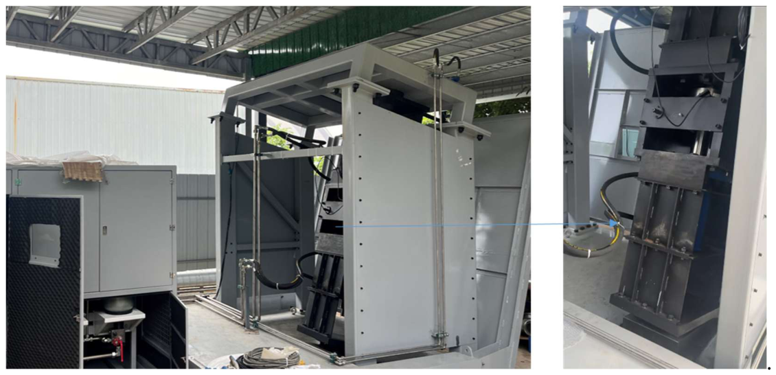
Figure 2.
Chord diagram of associations between fault events and monitoring signals.
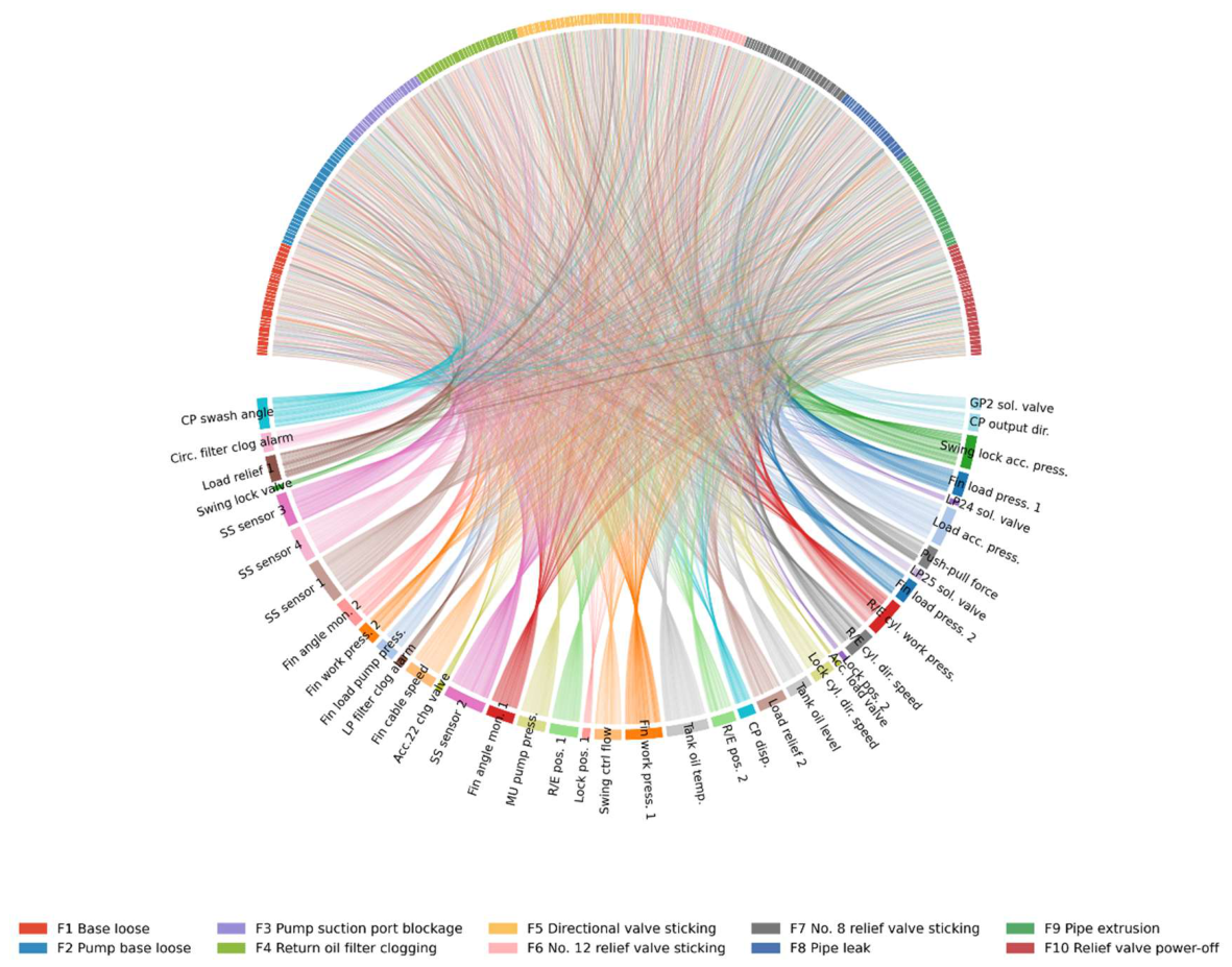
Figure 3.
Weight matrix and feature importance analysis.
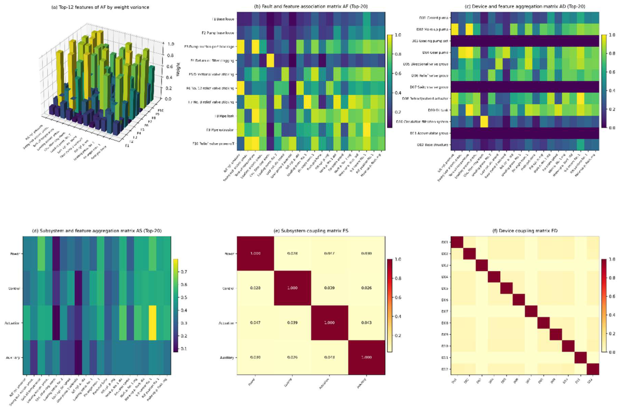
Figure 4.
Model performance comparison.
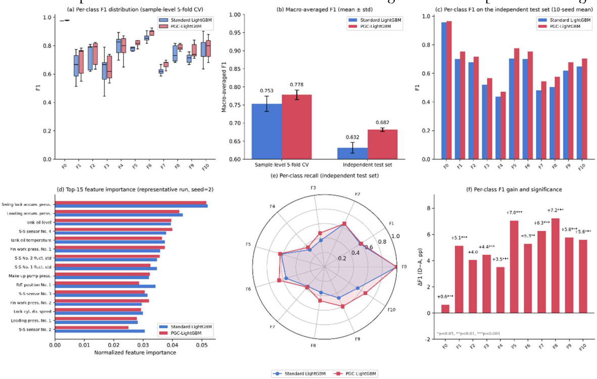
Figure 5.
Confusion matrices on the independent test set.
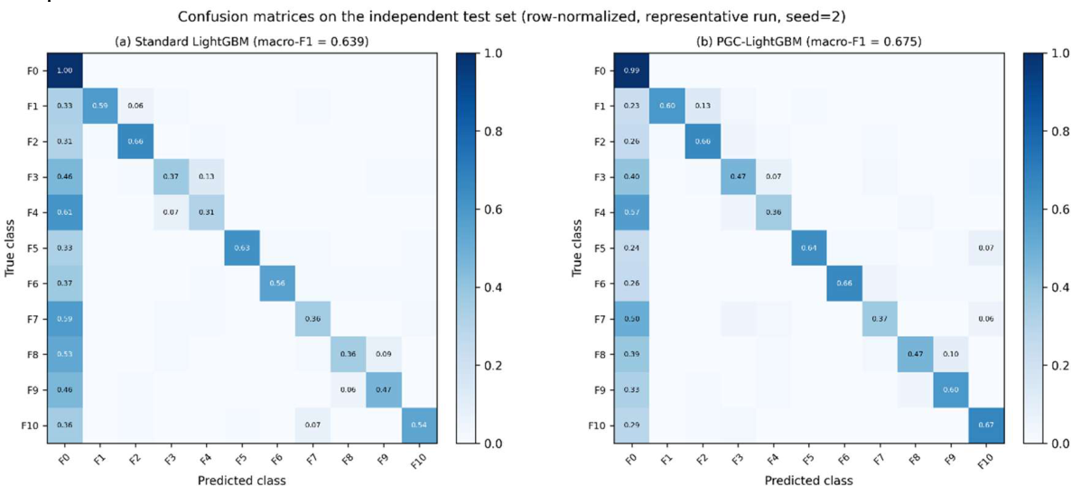
Figure 6.
Conformal prediction evaluation on the independent test set.
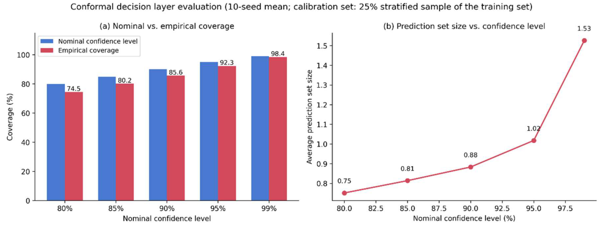
Table 1.
Sensor deployment of the hydraulic system.
| Sensor Type | Quantity | Measurement Position | Signal Type | Frequency (Hz) |
| Pressure sensor | 15 | Pump outlet, valve port, actuator chambers, return line | 4-20 mA | 1 |
| Flow sensor | 6 | Main supply line, branch lines | Pulse | 1 |
| Temperature sensor | 10 | Pump housing, oil tank, valve block, actuator | 4-20 mA | 1 |
| Vibration accelerometer | 8 | Pump housing (X/Y/Z), motor, valve body | IEPE | 25600 |
| Oil particle counter | 2 | Main return line, bypass filter circuit | RS485 | 0.2 |
| Current/speed sensor | 11 | Motor input, pump speed | 4-20 mA | 1 |
Table 2.
Inputs of the control circuit model.
| Sea state | Ship speed (kn) | Ship motion attitude 1 (deg) | OMEGA (rad/s) | Ship motion attitude 2 (deg) | OMEGA (rad/s) | Fin stabilizer attitude 1 (deg) | OMEGA (rad/s) | Fin stabilizer attitude 2 (deg) | OMEGA (rad/s) | Load cylinder curve (N) | OMEGA (rad/s) |
| 4 | 12 | 2.65 | 1.02 | 1.64 | 1.02 | 0 | 0 | 9.8 | 1.02 | 967.5 | 1.02 |
| 4 | 13 | 2.78 | 1.02 | 1.5 | 1.02 | 0 | 0 | 9.13 | 1.02 | 1034.78 | 1.02 |
| 4 | 14 | 2.98 | 1.02 | 1.36 | 1.02 | 0 | 0 | 8.31 | 1.02 | 1092.19 | 1.02 |
| 4 | 15 | 3.05 | 1.02 | 1.24 | 1.02 | 0 | 0 | 7.56 | 1.02 | 1140.85 | 1.02 |
| 4 | 16 | 3.17 | 1.02 | 1.13 | 1.02 | 0 | 0 | 6.89 | 1.02 | 1182.01 | 1.02 |
| 4 | 17 | 3.59 | 1.02 | 1.03 | 1.02 | 0 | 0 | 6.28 | 1.02 | 1216.89 | 1.02 |
| 4 | 18 | 3.77 | 1.02 | 0.9 | 1.02 | 0 | 0 | 5.74 | 1.02 | 1246.55 | 1.02 |
| 5 | 12 | 4.34 | 0.79 | 2.28 | 0.8834 | 0 | 0 | 12 | 0.8834 | 1158.99 | 0.8834 |
| 5 | 13 | 4.51 | 0.79 | 2.04 | 0.8834 | 0 | 0 | 10.78 | 0.8834 | 1221.46 | 0.8834 |
| 5 | 14 | 4.72 | 0.79 | 1.84 | 0.8834 | 0 | 0 | 9.69 | 0.8834 | 1273.75 | 0.8834 |
| 5 | 15 | 4.83 | 0.79 | 1.66 | 0.8834 | 0 | 0 | 8.48 | 0.8834 | 1317.61 | 0.8834 |
| 5 | 16 | 4.92 | 0.79 | 1.5 | 0.8834 | 0 | 0 | 7.89 | 0.8834 | 1354.58 | 0.8834 |
| 5 | 17 | 5.11 | 0.79 | 1.36 | 0.8834 | 0 | 0 | 7.15 | 0.8834 | 1385.93 | 0.8834 |
| 5 | 18 | 5.32 | 0.79 | 1.24 | 0.8834 | 0 | 0 | 6.51 | 0.8834 | 1412.69 | 0.8834 |
| 6 | 12 | 6.77 | 0.79 | 2.84 | 0.79 | 0 | 0 | 13.37 | 0.79 | 1291.15 | 0.79 |
| 6 | 13 | 6.89 | 0.79 | 2.53 | 0.79 | 0 | 0 | 11.88 | 0.79 | 1346.25 | 0.79 |
| 6 | 14 | 7.01 | 0.79 | 2.25 | 0.79 | 0 | 0 | 10.59 | 0.79 | 1392.05 | 0.79 |
| 6 | 15 | 7.13 | 0.79 | 2.02 | 0.79 | 0 | 0 | 9.48 | 0.79 | 1430.28 | 0.79 |
| 6 | 16 | 7.24 | 0.79 | 1.81 | 0.79 | 0 | 0 | 8.52 | 0.79 | 1462.38 | 0.79 |
| 6 | 17 | 7.35 | 0.79 | 1.64 | 0.79 | 0 | 0 | 7.68 | 0.79 | 1489.49 | 0.79 |
| 6 | 18 | 7.47 | 0.79 | 1.49 | 0.79 | 0 | 0 | 6.96 | 0.79 | 1512.54 | 0.79 |
Table 3.
Fault modes and main characteristics.
| Fault ID | Fault Name | Equipment | Main Characteristics |
| F0 | Normal operation | — | Parameters stable within design range |
| F1 | Base loose | Base mount | Increased vibration amplitude |
| F2 | Pump base loose | Pump mount | Abnormal pump alignment, noise increase |
| F3 | Pump suction port blockage | Pump inlet | Flow reduction, cavitation signatures |
| F4 | Return oil filter clogging | Filter | Increased return line back pressure |
| F5 | Directional valve sticking | Control valve | Extended response time |
| F6 | No. 12 relief valve sticking | Relief valve | Pressure regulation failure |
| F7 | No. 8 relief valve sticking | Relief valve | Pressure regulation failure |
| F8 | Pipe leak | Pipeline | Pressure drop, flow loss |
| F9 | Pipe extrusion | Pipeline | External force induced deformation |
| F10 | Relief valve power-off | Relief valve | System pressure loss |
Table 7.
Ablation experiment results.
| Configuration | Weighting scheme | Sample-level 5-fold CV | Independent test set |
| A | No weighting (baseline) | 0.753±0.021 | 0.632±0.015 |
| B | Class-balanced weighting | 0.768±0.018 | 0.668±0.004 |
| C | Fault-level physics-informed weighting | 0.772±0.025 | 0.682±0.006 |
| D | Full hierarchical weighting (proposed) | 0.778±0.013 | 0.682±0.005 |
Table 8.
Conformal decision layer evaluation on the independent test set.
| Nominal confidence level | Empirical coverage | Average prediction set size |
| 80% | 74.5% | 0.75 |
| 85% | 80.2% | 0.81 |
| 90% | 85.6% | 0.88 |
| 95% | 92.3% | 1.02 |
| 99% | 98.4% | 1.53 |
Disclaimer/Publisher’s Note: The statements, opinions and data contained in all publications are solely those of the individual author(s) and contributor(s) and not of MDPI and/or the editor(s). MDPI and/or the editor(s) disclaim responsibility for any injury to people or property resulting from any ideas, methods, instructions or products referred to in the content. |
© 2026 by the authors. Licensee MDPI, Basel, Switzerland. This article is an open access article distributed under the terms and conditions of the Creative Commons Attribution (CC BY) license (http://creativecommons.org/licenses/by/4.0/).
Copyright: This open access article is published under a Creative Commons CC BY 4.0 license, which permit the free download, distribution, and reuse, provided that the author and preprint are cited in any reuse.