
Submitted:
03 November 2026
Posted:
05 November 2026
You are already at the latest version
Abstract
The classical ecological theory of patch dynamics and community structure emerged in the early 1900s as a way to reconcile persistent patterns observed in the overall structure and function of forest and plant communities with continual change at the local or patch scale. The original theory was purely conceptual, but mathematical formulations based on Markov-chain models with empirical one-step transition probabilities began to appear in 1970. The main purpose of the present study is to incorporate three patch-scale ecological processes (succession, retrogression, and disturbance) into a Markov-chain model of patch dynamics, yielding a stochastic model that links patterns at the community scale to ecological processes acting at the patch scale. The main results deal with effects of the three patch-scale processes on the form of the stationary patch-state distribution and the length of time required to achieve approximate stationarity. The “forward” process of succession tends to concentrate patches near the ultimate successional state, while the “backward” processes of retrogression and disturbance tend to concentrate patches near the initial successional state; the form of the stationary patch-state distribution reflects the balance or imbalance between these processes. Frequent disturbance also tends to shorten the time required to achieve approximate stationarity.
Keywords:
community ecology
; spatiotemporal heterogeneity
; Markov chain
1. Introduction
The classical theory of patch dynamics and community structure in ecology emerged from a series of empirical studies of forest and plant communities conducted in the early 1900s. It was originally proposed as a way to reconcile the observed persistence of clear patterns in the overall structure and function of these communities with the continual change in physical structure and species composition observed at the local or patch level of organization. Influential papers by Cooper [6] and Watt [31] were noteworthy sources of the ideas underlying this theory.
Cooper studied a climax forest on Isle Royale in Lake Superior, one of the Laurentian Great Lakes in North America. He gives the following account of the patchy structure of the forest and the role of high-wind disturbance events in creating patches:
“The forest [on Isle Royale] is a complex of windfall areas of differing ages, the youngest made up of dense clumps of small trees, and the oldest containing a few mature trees with little young growth beneath... The forest in general is a mosaic or patchwork which is in a state of continual change. The forest as a whole remains the same, the changes in various parts balancing each other... [In other words,] the character of the forest as a whole is stable, though any given area is continually changing in composition and relative proportions of the various species.” (Cooper [6], pp. 43–44)
(Text in brackets was inserted by the present authors.) Since the “composition and relative proportions of the various species” characterize the state of any patch in the patchwork at any given time, an alternative way to express Cooper’s view is by saying that the character of the forest as a whole remains approximately constant, though the state of each patch is continually changing (Figure 1).
Watt, in a presidential address to the British Ecological Society, further develops the concept of plant and forest communities as mosaics of patches, where the overall structural pattern of the community is closely linked to the process-based dynamics observed within and among individual patches. He first presents a practical rationale for studying community dynamics in terms of the dynamics of patches:
“The ultimate parts of the community are the individual plants [and other associated organisms], but a description of it in terms of the characters of these units and their spatial relations to each other is impracticable at the individual level. It is, however, feasible in terms of the aggregates of individuals and of species which form different kinds of patches; these patches form a mosaic and together constitute the community. Recognition of the patch is fundamental to an understanding of structure as analysed here... The patches (or phases, as I am calling them) are dynamically related to each other [i.e., neighboring patches affect each other’s dynamics]. Out of this arises that orderly change which accounts for the persistence of the pattern in the plant community. But there are also departures from this inherent tendency to orderliness caused by fortuitous obstacles [e.g., random disturbance events] to the normal time sequence. At any given time, therefore, structure is the resultant of causes which make for order and those that tend to upset it. Both sets of causes must be appreciated.” (Watt [31], pp. 1–2)
Watt then presents his concept of forward and backward processes in patch dynamics:
“The cycle of change in all the communities [presented as examples in this address] is divisible into two parts, an upgrade and a downgrade. The upgrade series is essentially a process or set of processes resulting in a building up of plant material and of habitat potential and the downgrade a dispersion of these mainly by fungi, bacteria, insects, etc., but also by inorganic agents [e.g., fire or strong wind]. At each stage, of course, there is both a building up and a breaking down, but in the upgrade series the balance is positive, in the downgrade negative.” (Watt [31], p. 18)
Watt thought of the dynamics of patch state as being cyclical and referred to the different patch states (and sometimes the patches themselves) as phases. For example, in a plant community that he calls “Grassland A” (Watt [31], pp. 8–11), patches and their phases are associated with differences in microtopography that are created by a sequence of processes which operate during different phases, each preparing the way for the next phase:
- Phase 1:
- Plant colonization of low-elevation rocky patches (the hollow phase)
- Phase 2:
- Soil accumulation that increases patch elevation, accompanied by changes in species composition within each patch (the building phase)
- Phase 3:
- Continued increase in patch elevation and concomitant increase in the average spacing between plants (the mature phase)
- Phase 4:
- Further change in species composition within each patch, which causes increased erosion that begins to reduce patch elevation and increase plant mortality (the degenerate phase), eventually exposing the rocky substratum and regenerating the hollow phase.
Under this view, the process of returning from the mature phase of patch development to the initial (hollow) phase is an inherent part of the endogenous dynamics of patches rather than being caused by exogenous disturbance events such as fire or high-wind events. Cooper, by contrast, attributed returns from late to early stages of patch development to exogenous disturbance events.
Watt also argued that patches often do not develop independently. For example, in his description of what he calls the regeneration complex, he states: “Each patch in this space-time mosaic is dependent on its neighbours and develops under conditions partly imposed by them” ([31], p. 3). Cooper would likely have agreed with this intuitively plausible idea but does not address it.
None of the early (prior to circa 1950) forest and plant ecologists who proposed the original ideas for reconciling persistent patterns in overall structure of a community with the highly dynamic structures of its constituent patches expressed their ideas in the form of a mathematical model. To the best of our knowledge, the first such model to appear in the literature was a simple Markov-chain model of forest patch dynamics published in 1970 by two researchers (Stephens and Waggoner) at the Connecticut Agricultural Experiment Station [27,30]. Patches in the model were quadrats (belt transects) in four mixed-hardwood forests of central Connecticut (USA) in which all tree stems with breast-height diameters greater than 12 mm had been identified to species and counted in 1927, 1937, 1957, and 1967. Each quadrat in each observation year was classified into one of five mutually-exclusive categories based on the predominant tree species. These categories represented the possible states of each patch and together served as the state space for the Markov chain. One-step state-transition probabilities for a 10-year interval were estimated from the observed transitions in patch states between 1927 and 1937, and predicted four-step transition probabilites for the 40-year period between 1927 and 1967 were then calculated from the matrix of one-step transition probabilities on the assumption that the one-step transition probabilities remained constant during this period. The predicted 40-year state-transition probabilities were found to be rather similar to the observed proportions of patches that made the corresponding state transitions, suggesting that the Markov chain model might be a useful mangagement tool for predicting the dynamics of forest community structure.
Soon after the model of Stephens and Waggoner was published, a series of related models dealing with the dynamics of spatially heterogeneous communities subject to disturbance began to appear in the literature [8,10,12,13,18,19,28,29,34]. Most of these models represent the dynamics of each patch as a Markov chain. As noted above, the Stephens-Waggoner model of forest succession employed patches that contained numerous individual trees. Horn [13] proposed an alternative Markov-chain model of forest succession based on a grid or honeycomb of small patches, each containing either a single individual tree or no trees at all. A roughly similar approach was applied by Lippe et al. [19] to a heathland plant community, and by Tanner et al. [28] and Hill et al. [12] to marine communities dominated by sessile invertebrates.
In all of these models, the assumed Markov chain represents the dynamics of a single patch. Interpretation of the state probabilities for an individual patch as proportions of all patches in the community is then based on two additional simplifying assumptions: that different patches are stochastically independent (including disturbance events that act on them), and that the total number of patches in the community is large enough so that, by the laws of large numbers, the proportion of patches that will be in any particular state at any particular time is well approximated by the probability of a representative patch being in that state at that time.
New contributions to this series of published models have continued to appear in the literature to the present day and target a variety of different types of communities, including terrestrial plant and forest communities, marine rocky intertidal communities, and stream benthic communities. Like the original model of Stephens and Waggoner, the subsequent models deal with communities whose overt physical structure is dominated by species in which reproductive individuals are sessile or exhibit only very limited mobility. These models also implicitly assume that patches within a given community are subject to a continual rain of dispersal propagules that enter from outside the community. These assumptions restrict the domain of applicability of the models but are reasonable simplifications for many communities. For example, seeds from considerable distances may be transported to patches in a forest or plant community by a variety of physical and biological vectors, then accumulate over time in a seed bank and remain viable for long periods of time, awaiting appropriate environmental cues (e.g., increased light in a forest patch after a tree falls, creating a canopy gap) to initiate germination and growth. And in rocky intertidal and stream habitats, dispersal propagules continually settle from the water column onto the substrate within a given patch after being transported by water currents from distant locations.
A significant limitation of these models, from the perspective of ecological theory, is that all of them — with the possible exception of Horn’s model — are strictly empirical in the sense that they treat the one-step state-transition probabilities for a patch simply as statistical parameters to be estimated from a large number of observed state transitions instead of proposing a set of underlying ecological processes from which quasi-mechanistic formulas for these probabilities are derived. In the present paper, we propose a new addition to this series of Markov-chain models of patch dynamics and community structure that addresses this limitation in a simple and practical way. Drawing upon the ideas of Cooper [6] and Watt [31] outlined above, we develop and analyze a model that can be viewed as a process-based extension of the discrete-time Markov-chain model originally proposed by Stephens and Waggoner [27] and Waggoner and Stephens [30]. As is true of the other stochastic models of patch dynamics and community structure in this series, the model we propose is intended for application to terrestrial and aquatic communities occuring on firm substrates (e.g., soil in terrestrial environments, rocks in the rocky intertidal zone, stones in a stream bed), whose most conspicuous members are sessile or have only very limited mobility. A key process organizing such communities is competition for space that individuals of the most conspicuous taxa require in order to access limiting resources such as light, nutrients, or suspended food particles. A unique feature of the model we propose is that its one-step state-transition probabilities for a patch explicitly represent the effects of three general types of patch-scale ecological processes: succession (an endogenous upgrade process, in Watt’s terminology), retrogression (an endogenous downgrade process), and disturbance (an exogenous downgrade process).
The remainder of this paper is organized as follows. Section 2 defines several ecological terms and mathematical symbols we will use. Section 3 presents the model and analytical results in detail. The main results are then illustrated with numerical examples in Section 4. We close with a brief summary of the main results and discussion of some limitations of classical stochastic models of patch-dynamics and community structure in Section 5.
2. Terminology and Notation
2.1. Terminology
Here we clarify our usage of several ecological terms whose definitions vary in the literature vary, beginning with community. As Ricklefs ([25], p. 669) notes, “the term community has been given such a variety of meanings by ecologists [and taxonomic specialists with an interest in ecology] that it borders on being meaningless.” We adopt a functional rather than descriptive or taxonomic definition of this term. Thus, by a community, we mean all the interacting populations of organisms living together in a particular area, without restriction to any particular taxonomic or quasi-taxonomic group (e.g., diatoms, algae, benthic insects, fish, trees) or growth habit (e.g., periphyton). In practice, spatial and taxonomic community boundaries are set partly for practical purposes but always enclose an area occupied by numerous individuals of multiple species, where the key interspecific interactions that influence the dynamics of abundance (competition, predation, herbivory, etc.) occur mainly within the community.
We refer to the more-or-less homogeneous physical environment in which a community exists as a habitat. Thus, a community is all the interacting populations of organisms living in a particular habitat. It will sometimes be convenient to refer to a plant community, a stream epilithic algal community, and so on, and when we do so, we mean a community whose most conspicuous or prevalent members are plants, epilithic algae, etc., but which also includes many other taxa. In our usage, then, the plants alone or epilithic algae alone constitute an assemblage or association, not a community (cf. Ricklefs [25], pp. 669–670).
By disturbance, we mean any exogenous process or event that opens a spatial gap in the community by killing or removing individuals, or by exposing new inhabitable surfaces for colonization. Examples include fire and high-wind events in terrestrial forest and plant communities, high-flow events in streams, and high-energy wave events in the marine intertidal zone. Contrary to a definition of disturbance sometimes encountered in the ecology literature (e.g., [26]), natural endogenous mortality — for example, due to old age, or to grazing or predation by a species that is a community member — is not disturbance under our definition. Thus, as we use the term, disturbance is necessarily an exogenous process, and existence of a community that is free of disturbance is therefore conceptually possible.
Two main methods for representing spatial heterogeneity have been employed in published analytical stochastic models of community dynamics. With the first method, the fundamental community subunits are patches that comprise multiple individuals of multiple species but whose abundances are not explicitly represented in the model (e.g., [8,10,27,29,30]). In the second method, the fundamental subunits are single individuals with fixed locations, or small spatial patches occupied by no more than one individual (e.g., [12,13,19,28]). Thus, the first method employs multi-individual patches while the second employs single-individual patches. We use the first method to represent spatial heterogeneity in the model we pose and analyze in the present paper.
Following Watt [31] and numerous subsequent authors (e.g., [8,10,11,17,18,21,32]), we view a patch as a discrete area within a habitat. We note, however, that there is no general agreement in the literature as to how patches are delineated. In some cases, patches represent recognizable physical units that exist independently of any organisms that may inhabit them (e.g., stones in a stream bed). In other cases, patches are notional entities whose boundaries are created by an investigator for purposes of sampling (e.g., sampling quadrats) or by the spatial resolution of raster satellite imagery. In still other cases, patches are spatial gaps created within a community by disturbance events (e.g., gaps in a forest created by fire or wind). The model we study in this paper employs patches with boundaries that are viewed as fixed and independent of disturbance, as in the first and second types of patch just mentioned. The third type of patch — those whose boundaries are created by disturbance events — is more difficult to represent adequately in an analytically-tractable stochastic model, and we know of no examples of such a model in the literature. We view patches as being contiguous or nearly so, and much smaller in size than the habitat in which they are located, and we refer to the portion of a community located within a patch as a subcommunity. In our terminology, then, each habitat contains a single community, each community is composed of multiple subcommunities, and each subcommunity occupies a single patch within a habitat (Figure 2).
The temporal process of change in a patch (subcommunity) following a disturbance event is an important part of the model we develop and analyze in this paper. Following Watt [31], we split this process of change into two parts: a “forward” part and a “backward” part (recall that Watt called these “upgrade” and “downgrade” parts). We refer to the forward part as succession, in accordance with modern usage of that term (e.g., [5,29]), and we refer to the backward part as retrogression (not to be confused with various uses of this term in the classical literature on succession in plant communities as discussed, for example, by Clements [3]), which essentially resets patches to earlier successional stages. Thus, our model includes one forward or upgrade process (succession) and two backward or downgrade processes (retrogression and disturbance). We view both succession and retrogression as endogenous processes governed mainly by different networks and intensities of interspecific interactions that occur in patches at different successional stages; disturbance, by contrast, is an exogenous process.
Though our patch-based modeling approach does not address individual species, it nevertheless implicitly assumes that new species added to patches (subcommunities) during succession originate outside the focal community and are transported to individual patches by a colonization or invasion process that occurs at all successional stages but whose probabilities of successful establishment for different species vary with species and successional stage. This assumption is often plausible, for example, in stream benthic communities, where dispersal propagules originate well upstream of the focal community, are transported downstream by the current, and settle in patches from the drift. In such cases, the physical transport process that constantly delivers new candidate species to patches is exogenous, but the success or failure of different invading species in becoming established members of any given subcommunity is determined by endogenous processes and changes during succession.
The stream epilithic algal communities addressed by DeNicola et al. [8] illustrate the meaning of these terms. As background, stream ecologists commonly measure what is known as community metabolism by recording time series of dissolved oxygen (DO) concentration, water temperature, photosynthetically active solar radiation, and possibly other physicochemical properties in one or more stream segments, each of whose boundaries are chosen so the segment has reasonably uniform thalweg current speed, water depth, and degree of shading. These segments correspond to habitats in our terminology. Using the time-series data in conjunction with a model of stream DO dynamics and an appropriate statistical estimation method, the main components of community metabolism (community gross and net primary production, and community respiration) are estimated for each segment (for details, see [1,9,20]). Thus, from the perspective of stream function, it is natural to think of a community as the collection of all taxa in a given segment (habitat) that have a significant direct (e.g., epilithic algae) or indirect (e.g., benthic invertebrate grazers on epilithic algae) effect on DO dynamics in the segment and hence on estimates of community metabolism. The collections of taxa occurring on individual stones (patches) in the stream bed of a segment are the “tiles” of the community mosaic and therefore are naturally termed subcommunities. The main source of disturbance considered by DeNicola et al. [8] is high-flow events that scour algae and other benthic organisms from stones or expose the bare undersurfaces of stones by overturning them. In the absence of grazing by benthic invertebrates, the subcommunities on individual stones exhibit a reasonably well-defined process of development following each disturbance event, the details of which depend on light and nutrient levels in the habitat. For example, when light and nutrient levels are high, biomass accumulates and taxa with high-profile growth forms become more abundant, creating a subcommunity with a complex three-dimensional physiognomy (see DeNicola et al. [8] for more details). It is reasonable to think of this process as a forward or upgrade process and to refer to it as succession. When benthic invertebrate grazers encounter a subcommunity on a stone that has progressed to one of the later stages of succession, they may consume a significant portion of the biomass that has accumulated since the last high-flow event, creating a more two-dimensional subcommunity that is low in biomass and dominated by taxa with low-profile growth forms, in effect returning the subcommunity to an earlier successional stage. These grazing invertebrates are an integral part of the stream’s epilithic algal community, so their impact on a given patch is not disturbance. Instead, we view it as an endogenous backward or downgrade process and refer to it as retrogression. Much like grazing events, disturbance events also may cause a significant reduction in algal biomass on individual stones, along with changes in physiognomy and taxonomic composition, effectively returning the subcommunity to an earlier successional stage. Thus, patch dynamics in the model are the result of three ecological processes: succession, retrogression, and disturbance.
The model we study in this paper is posed in discrete time. Patches are assumed to be observed at regularly-spaced times, with the state of each patch in the habitat being recorded at each observation time. By the state of a patch, we actually mean the state of the subcommunity within the patch. There are various ways to define the state of a patch. For complex natural communities where patches may contain hundreds of species and vastly larger numbers of individuals, a particularly useful way — as Watt [31] points out — is to define a small number of discrete classes that are easily recognizable by an investigator and include all possible configurations of a patch. For example, Stephens and Waggoner [27] and Waggoner and Stephens [30] define five patch states in their study of a forest community, based on the tree species with the largest number of stems in a patch: Maple, Oak, Birch, Other Major Species, and Minor Species. Fisher et al. [10] define six patch states in their study of a desert stream algal community: bare sand, four states dominated by different algal groups, and algae stranded on dry stream banks following high-flow events. And DeNicola et al. [8] define nine patch states for stream epilithic algal communities: bare substratum and eight patch types based on the dominant growth form of algal taxa within the patch. With this scheme of observation times and patch states, the dynamics of a patch consists of a temporal sequence of observed states, each of which is a member of the set of all possible patch states, which we call the patch state space.
2.2. Notation
In developing the model, it is necessary to specify various subsets of the integers and real numbers. The following symbols are useful for this purpose:
| , |
| for and , |
| the set of all real numbers, |
| . |
The Kronecker delta function is denoted by , which is defined for integers i and j in an appropriate subset of by
The following matrix notation is used. Except when the elements of a vector or matrix are all 0 or all 1, vectors are denoted by boldface lower-case Roman letters and are assumed to be column vectors except when specifically identified as row vectors by a superscript “T” indicating the transpose of a column vector. Matrices with at least 2 rows and at least 2 columns are denoted by boldface upper-case Roman letters. Thus, denotes a column vector, denotes a row vector, and denotes a matrix with at least 2 rows and at least 2 columns. In the special case where the elements of a vector or matrix are all 0 or all 1, the vector or matrix is denoted by or ; whether these symbols represent a vector or a non-vector matrix will be clear from the context. Elements of vectors and matrices are labeled with indices in or , where C is a positive integer (see below). Finally, denotes the unit vector with elements or , where for and for all . Thus, if the index set is , then
where k is a fixed integer in .
3. The Model
3.1. Basic Model Structure
As noted above in Section 2.1, we will consider situations where there are two main spatial/biological scales: the habitat/community scale and the patch/subcommunity scale, with each habitat comprising multiple patches, and each community comprising multiple subcommunities. In applications, it may sometimes be desirable to include lower biological scales than the subcommunity (e.g., the individual or population scale) or higher spatial/biological scales than the habitat/community (e.g., the reach or catchment scale in streams). We do not, however, deal with these additional scales here (potentially useful approaches for applications involving these scales include individual-based simulation models [7], metapopulation models [11], and metacommunity models [17]).
The state space for each individual patch is the finite set of integers defined by
where state 0 is the state resulting from disturbance and states are stages in community succession. The habitat comprises n patches labeled , each of whose state is an element of . There are various ways that the state of a habitat can be characterized. An obvious one is to keep track of the state of every individual patch in the habitat. However, we will use an alternative method that we feel is more practical and aligns better with empirical approaches that have been employed in the literature: we will keep track of the number of patches in each of the possible patch states. The state space for the habitat is then the finite set of vectors defined by
where denotes the number of patches in patch state i.
We assume that a disturbance event, such as a high-wind event in a forest, re-sets the state of each affected patch to state 0, regardless of its state immediately prior to the event. We further assume that disturbance is the only process that can transform a patch to state 0. We refer to state 0 as the disturbed state (or the null successional stage) and to states as successional stages, with state C being the climax stage (see below).
We pose the model in discrete time. Patch and habitat states are assumed to be observed at equally-spaced times , where [dimension: Time] is the length of each inter-observation period and [dimensionless] is the number of inter-observation periods that have elapsed. We will refer to as the m-th observation time, and to m as the time step. To avoid the dimensional confusion that often arises in discrete-time models, it is important to distinguish between dimensional quantity and dimensionless quantity m. In discrete-time dynamics, the key variable typically is the dimensionless number m of time steps, with dimensional time entering only indirectly through the relationship, .
As noted in the Introduction, we view community dynamics as the stochastic outcome of three patch-scale processes: succession, retrogression, and disturbance. Succession is the only “forward” or “upgrade” process we consider, while both retrogresion and disturbance are “backward” or “downgrade” processes that interrupt succession and reset it to earlier stages. We assume that if there were no backward processes, succession would inevitably culminate in a so-called climax community (state C). For simplicity, we assume here that the climax community is unique, though the theoretical framework we develop can accommodate two or more alternative climax states.
As is typical of discrete-time models for processes that in reality occur in continuous time, the ability to think clearly about the effect of each individual process is greatly improved by assuming succession, retrogression, and disturbance act sequentially rather than simultaneously. Therefore, during the open interval between any two consecutive observation times and , we assume that succession acts first, then retrogression, and then disturbance (Figure 3). The final outcome of the sequential action of these three processes in any given patch between observation times and determines the state of the patch at observation time and time step .
To facilitate analytical study of the main properties of the model while avoiding unnecessary complications, we make the following simplifying assumptions regarding the processes of succession, retrogression, and disturance during the open interval between any two consecutive observation times and :
- 1.
- Succession phase: A succession event occurs or fails to occur in any given patch independently of events in other patches. If it occurs in a given patch, it causes the patch state to advance to the next successional stage (unless the current state is C); if it fails to occur, the patch retains the state it had at observation time .
- 2.
- Retrogression phase: A retrogression event also occurs or fails to occur in any given patch independently of events in other patches. If it occurs in a given patch, it causes the state of the patch to regress to the previous successional stage (unless the previous stage is state 0); if it fails to occur, the patch retains the state it had at the end of the succession phase. Retrogression includes effects of various endogenous processes such as mortality due to predation or herbivory, and natural age-related mortality; it excludes mortality caused by disturbance events.
- 3.
- Disturbance phase: As with succession and retrogression, a disturbance event occurs or fails to occur in any given patch independently of events in other patches. If it occurs in a particular patch, it causes the patch state to transition to state 0 (or as Horn ([13], p. 204) puts it, the patch is “crushed by the hand of fate”), regardless of the current state; if it fails to occur, the patch retains the state it had at the end of the retrogression phase. The state of the patch at the end of the disturbance phase becomes the state at observation time and time step .
A visual representation of the effects of succession, retrogression, and disturbance on patch states in a simple community with patches is provided in Figure 4.
Two additional assumptions that are important in simplifying the model and facilitating its analysis are the following. First, consistent with Watt’s theory of patch dynamics and community structure, classical disturbance theories of forest ecology (e.g., Cooper [6]), and most previous stochastic models of disturbance effects in spatially heterogeneous communities (but not with the model of DeNicola et al.[8]), we assume that succession, retrogression, and disturbance all act at the patch scale. Second, consistent with most previous stochastic models (but not with Watt’s [31] theory), we assume these processes act independently in different patches.
Random variable represents the state of patch k at observation time and time step m. Under our simplifying assumptions, the stochastic dynamics of for any patch k are independent of the dynamics of every other patch. We further assume that stochastic process , taking values in patch state space , is a discrete-time Markov chain. The patch-state probability distribution of the Markov chain at observation time and time step m is represented by vector , where . The one-step transition-probability matrix is , where for any pair of consecutive observation times and and time steps m and . Two fundamental assumptions of the type of Markov chain we employ are that the one-step transition probabilities do not change over time, and the probability that any given patch will be in state j at observation time may depend directly on which state the patch was in at observation time but may not depend directly on which state the patch was in at any observation time prior to . That is,
We note that, though the notation conceals it, one-step transition probabilities implicitly depend on the duration of the period between successive observations.
At the habitat scale, random variable represents the number of patches that are in patch state i at observation time and time step m, and vector-valued random variable represents the corresponding state of the habitat.
3.2. One-Step Transition-Probability Matrices
3.2.1. Succession
The one-step transition-probability matrix for succession is , where element is the probability that any given patch that is in state i at observation time , for any time step m, will be in state j at the end of the subsequent succession phase. Thus, the probability distribution for the state of an individual patch at notional time is given in terms of the probability distribution for the state at observation time by
We assume the succession process acting between times and on any patch whose state at was i succeeds in advancing the state to with probability () and fails to change it with probability , unless the patch was in state C before succession acted. In the latter case, we assume succession cannot change the state of a patch that is in climax state C, meaning . The full set of one-step transition probabilities for succession is given by
The pattern of zero and nonzero transition probabilities is more evident when stochastic matrix is expressed in matrix notation:
Note that is triangular, implying . The corresponding directed graph (i.e., one-step state-transition diagram) for succession is shown in the first (top) row of Figure 5.
3.2.2. Retrogression
The one-step transition-probability matrix for retrogression is , where element is the probability that any given patch that is in state i at time , for any time step m, will be in state j at the end of the subsequent retrogression phase. Thus, the probability distribution for the state of an individual patch at notional time is given in terms of the probability distribution for the state at notional time and the probability distribution for the state at observation time by
We assume the retrogression process acting on any patch whose state whose state at was i succeeds in causing the patch to regress to state with probability () and fails change it with probability , unless the patch was in state 0 or 1 before retrogression acted. In these latter cases, retrogression cannot occur (), because there is no successional state prior to state 0, and disturbance is the only process that can cause a transition to state 0 from any other state. The full set of one-step transition probabilities for retrogression is given by
In matrix notation, stochastic matrix has the simple form,
Note that is triangular, whence . The corresponding directed graph for retrogression is shown in the second row of Figure 5.
3.2.3. Disturbance
The one-step transition-probability matrix for patch-scale disturbance is , where element is the probability that any given patch that is in state i at time , for any time step m, will be in state j when the disturbance phase ends at observation time . Thus, the probability distribution for the state of an individual patch at observation time is given in terms of the probability distribution for the state at notional time and the probability distribution for the state at observation time by
We assume the disturbance process acting on any patch whose state at was i succeeds in causing the patch to transition to state 0 with probability () and leaves the state unchanged with probability , unless the patch was already in disturbed state 0 before disturbance acted. In the latter case, we assume the patch remains in state 0 with probability 1. (Note that these assumptions imply a severe form of disturbance; milder forms would not necessarily return patches all the way to state 0, and their effects would be similar to those of retrogression.) The one-step state-transition probabilities for the disturbance process are therefore given by
Written as a matrix, stochastic has the form
The corresponding directed graph is shown in the third row of Figure 5. Note that is a triangular stochastic matrix, with . A suggestive alternative expression for is the following:
where is the identity matrix and is a partitioned matrix whose first column () is a vector of ones and whose remaining C columns () form a matrix of zeros.
A useful property of matrices and is that they commute under matrix multiplication, meaning that (Appendix A). The significance of this property will become apparent below (Section 3.6) when we assess the effects of changing the order in which succession, retrogression, and disturbance are assumed to act during the interval between consecutive observation times.
3.3. Succession and Retrogression Combined
The one-step transition-probability matrix for the sequential effects of succession and retrogression within an individual patch has the tridiagonal form,
3.4. Succession, Retrogression, and Disturbance Combined
The one-step transition-probability matrix for the sequential effects of succession, retrogression, and patch-scale disturbance is , where is the probability that any given patch that is in state i at observation time will be in state j at observation time for any time step m. Using Eqs. (11) and (10), the general form of is given by
For example, in the special case where ,
Returning to the general case, we have . The directed graph is shown in the bottom row of Figure 5.
Three properties of matrix will be important below. First, note that all elements of are nonnegative, and all row sums equal 1. These facts imply that is a stochastic matrix, which in turn implies that is an eigenvalue of and also is the spectral radius, and that is a right eigenvector corresponding the . These three closely-related facts constitute the first important property of . Next, the directed graph of in Figure 5 shows that is strongly connected (i.e., any state can be reached from any other by a directed path of finite length). This fact implies that is irreducible ([14], Theorem 6.2.24, p. 403), which is the second important property of . Finally, this property and the fact that all main diagonal elements of are strictly positive imply that for all ([14], Lemma 8.5.4, p. 541). This fact in turn implies that is primitive ([16], p. 546) and aperiodic ([2], p. 374), which together are the third important property of .
3.5. Patch-State Dynamics
The one-step transition-probability matrix for changes in the state of a patch between any two consecutive observation times is . From Eq. (7), the patch-state probability distrribution at observation time can be expressed in terms of the patch-state probability distrribution at observation time and one-step transition-probability matrix as
which is a homogeneous first-order linear recurrence relation with constant coefficients. Iterating, its solution is found to be
where initial patch-state probability distribution is arbitrary (except that its elements must be nonnegative and sum to 1) and is assumed to be given.
The behavior of as is determined by properties of matrix , which in turn are determined by the eigenvalues and the left and right eigenvectors of . For example, if all eigenvalues are distinct (as they are in all the numerical examples presented below in Section 4), can be expanded in terms of the m-th power of its eigenvalues as
where and are the right and left eigenvectors of corresponding to eigenvalue , normalized so that for all i. The eigenvalues are labeled in order of decreasing modulus, so that . Because is stochastic, , , and for all i. In fact, by the strong form of the Perron-Frobenius theorem, the fact that is primitive implies that for all , and therefore for all . It follows that as . Moreover, the rate at which this convergence occurs as the number m of time steps increases is clearly determined mainly by how small the second-largest modulus of the non-unit eigenvalues is; the smaller is, the faster converges to its limit .
The key implications of these properties of are the following, which we paraphrase from Theorem 5.1 of Çinlar ([2], pp. 378–379). Because is irreducible, primitive, and aperiodic, all rows of matrix converge to the same positive row vector as , which is the unique solution of the system of linear equations,
The convergence is geometric in m, meaning there are constants and such that
for all rows i and columns j of and all elements j of . (It suffices to choose as the second largest modulus of the eigenvalues of .) It follows that in Eq. (14),
independent of the choice of , where the convergence is geometric in m.
In words, these results mean that patch-state probability distribution converges geometrically to a unique stationary distribution , all of whose elements are positive. Distribution is called stationary because, if at some observation time , then Eqs. (13) and (16) imply that for all future observation times . Moreover, convergence to the same stationary distribution occurs for any initial distribution , so the stationary distribution is also asymptotically stable.
Let denote the minimum (possibly fractional) number of time steps required for the upper bound on the right side of Eq. (18) to be reduced to proportion () of , with chosen as the second-largest modulus () of the eigenvalues of one-step transition-probability matrix and ignoring the restriction of m to the integers. Then
For convenience, we will refer to [dimensionless] as the STEAS index (Steps To Ensure Approximate Stationarity), where the word “ensure” is meant to indicate that the index applies to all possible initial states of a patch (the number of steps required to achieve stationarity is obviously 0 if the initial patch-state probability distribution is chosen as ). Various other indices are available for characterizing how quickly or slowly a Markov chain is guaranteed to achieve approximate stationarity, and all of them usually produce roughly similar results. However, we find the interpretation of STEAS particularly simple and clear.
To derive an explicit formula for , we may rearrange Eq. (16) to obtain
Because is an eigenvalue of , is singular and therefore cannot be inverted. Define vector by . Adding to both sides of Eq. (21), using Eq. (17), and solving the resulting system of linear equations uniquely for yields
where .
3.6. Effects of Different Orderings of Succession, Retrogression, and Disturbance
A drawback of posing the Markov-chain model for patch dynamics in discrete time is that one must assume an arbitrary order in which succession, retrogression, and disturbance act between any two consecutive observation times. The question arises, then, as to whether different orders would produce qualitatively different results. As the numerical examples presented below in Section 4 illustrate, the answer is that the same qualitative relationships between the stationary patch-state distribution and the one-step probabilities of succession, retrogression, and disturbance typically will hold for all possible orderings of these three processes. The main reason this is so is that, although the six possible orderings of these processes yield somewhat different forms of the one-step transition-probability matrix , all six forms of have exactly the same eigenvalues (the mathematical basis of this property is outlined in Appendix A). As a result, the convergence to a stable, stationary patch-state distribution indicated by Eq. (19) holds in all six cases, and the numerical value of STEAS index is exactly the same. The form of the stable patch-state distribution differs somewhat between cases, because the form of matrix in Eq. (16) differs. But numerical examples for the six possible orderings of succession, retrogression, and disturbance using the same sets of values for probabilities s, r, and that are used in Figure 6 (two of which are presented in Appendix B) suggest that the qualitative effects of these three processes on the form of will remain the same, at least for values of s, r, and that that are not close to 0 or 1.
3.7. Habitat-State Dynamics
The Markov chain for the state of each of the n patches in a habitat is assumed to be independent of the Markov chain for the state of every other patch. It follows that the habitat state at observation time and time step m has a multinomial distribution with n “trials”, each with possible outcomes (labeled ) whose probabilites are given by . Let denote the probability that , with the probability vector for the initial state of each patch being . Then,
where .
For sufficiently large m (and hence ), we have for all (because is nonnegative and aperiodic and therefore for all sufficiently large m). Moreover, as , these probabilities approach a stationary distribution given by Eq. (22), and therefore approaches the limiting form given by
This result implies that the sequence of vector-valued random variables for converges in distribution to random variable as , where the probability that is given by .
Expressions for various moments of the habitat state distribution follow at once from the multinomial distribution in Eq. (23). These moments are well known but can be efficiently derived from the moment generating function defined by
where is a vector of real-valued parameters (one for each possible patch state) and the summation extends over all values of that sum to n. We are particularly interested in the mean and variance of the number of patches in any given state i at any given observation time , and in the covariance of and for different patch states . It follows from Eq. (25) that for any fixed number n of patches,
Note that, although the Markov chains in any two patches are stochastically independent, there nevertheless is a negative covariance between the numbers of patches in different states, because the total number of patches is finite (e.g., if all n patches were in state i at time , none could be in any state ).
The above formulas for the moments of lead at once to the following results for moments of the proportion of patches in any state i for fixed observation time and time step m:
Thus, for a habitat with a sufficiently large number n of patches, the proportion of patches in any state i will be approximately at any observation time, and the variance and covariance of proportions and will be close to zero. These results are consistent with Cooper’s [6] idea, based on his study of the Isle Royale forest, that structural and functional properties at the community/habitat scale remain approximately constant, despite continual change at the subcommunity/patch scale (Figure 1).
4. Numerical Results
We now present several numerical examples to illustrate the effects of succession, retrogression, and disturbance on the form of the stationary patch-state distribution , the associated diversity of patch states, and the number of time steps required for the time-dependent distribution to achieve approximate stationarity. To give a clear sense of the overall or main effects of these processes with a reasonable number of examples, we restrict attention to the special case where each process acts with the same probability on every patch, regardless of its state. That is, we assume in Eq. (2) and in Eq. (5) for all states i. All computer programs were written in the R programming language ([22], version 4.6.2).
The stationary patch-state distributions for 20 combinations of one-step succession probability s, retrogression probability r, and disturbance probability are presented graphically in Figure 6. Each panel in the figure corresponds to a different combination of these three probabilities. The panels are arranged in four rows and three columns; the corresponding values of s, r, and are listed at the top of each panel and in Table 1. The five panels in each row of the figure share the same value of , which increases from top to bottom rows. The four panels in each column share the same combination of s and r values, with s increasing and r decreasing from the left to right columns in such a way that in the left column, in the middle column, and in the right column. Thus, disturbance events become more prevalent from top to bottom rows in the table, while succession events become more prevalent and retrogression events become less prevalent from left to right columns. Another useful intuitive interpretation of the columns is that retrogression dominates succession () in the left column, succession dominates retrogression () in the right column, and the two processes are balanced () in the middle column.
We supplement the stationary patch-state distributions with corresponding values of Shannon’s information-theoretic entropy index H, given by
This index represents the amount of patch-state information that would be conveyed by determining the state of a single patch that was randomly sampled from a population with known proportions of its patches in states (Khinchin [15] gives a lucid treatment of the theory underlying Shannon’s index and its interpretation as an index of entropy, uncertainty, and information). Consistent with intuition, the amount of information conveyed is zero if all patches have the same state (i.e., for some state , and for all ), because we know without determining the state of the chosen patch that its state must be . In this case, (to derive this result, terms with on the right side of Eq. (32) are interpreted as their limit as , which is 0.) At the opposite extreme, the amount of information conveyed is greatest for a given number of patch types if all patch states are equally likely to be chosen (i.e., for all i), in which case .
As these extreme cases suggest, low values of H indicate a patch-state distribution that is concentrated around a single state, while high values indicate a relatively even distribution. These properties make H a useful index of patch-state diversity. Values of H for the 9 stationary distributions shown in Figure 6 (as well as several other values) are listed in Table 1. Note that patch-state diversity tends to be highest when the disturbance probability is low and succession and retrogression are balanced, or when the disturbance probability is high and the succession probability significantly exceeds the retrogression probability. The relationship between patch-state diversity H and disturbance probability , as well as the dependence of this relationship on succession and retrogression probabilities s and r, is illustrated in Figure 7. Note that in each of the five examples shown in this figure, H is maximal at an intermediate level of disturbance, providing an interesting analog of the intermediate disturbance hypothesis for species diversity [4,13,33].
The form of the stationary distribution provides no information about how many time steps are required in order to ensure that the current patch-state probability distribution closely approximates stationary distribution for all possible choices of the initial patch-state distribution. This information is important, because the longer the time required to ensure approximate stationarity following disturbance events, the less likely it is that the patch-state distribution of the community within a habitat will resemble its stationary configuration at a given observation time. To provide this type of convergence-time information, we calculated values of STEAS index , defined in Section 3.5, corresponding to the various stationary patch-state distributions shown in Figure 6. These values are presented in Table 1; values for a larger number of choices of probabilities s and r are plotted in Figure 8. Because the eigenvalues of are the same for all possible orderings of succession, retrogression, and disturbance, the values of in Table 1 and Figure 8 also hold for all possible orderings of these three processes. Note that the number of time steps required to ensure approximate stationarity is greatest when succession and retrogression are balanced and the prevalence of disturbance is low, and that increasing the prevalence of disturbance decreases the required number of time steps. (For fixed choices of s and r, the number of time steps required to ensure approximate stationarity will increase if the number of successional stages is increased; the numerical results we report assume a fixed number of successional stages.)
The accelerating effect of larger values of disturbance probability on covergence to the stationary patch-state distribution is illustrated more directly in Figure 9. Each of the four plots in this figure shows patch-state distribution at time steps (on the horizontal axis). Succession and retrogression are balanced () in all four cases, and the patch state at initial time step is 1. The four plots differ only in the value of , which increases from the top plot () to the bottom plot (). The segment heights within each bar represent the probabilities of different patch states, with states 0 through 8 being indicated by increasingly darker shades of green (white for state 0, dark green for state 8). The value of STEAS index is also displayed at the top of each bar plot. Note that the number of time steps required for the patch-state distribution to roughly stabilize clearly decreases from the top to the bottom plots as increases from to . The corresponding values of as decrease from to .
5. Discussion
The numerical results of Section 4 show that the stationary patch-state distribution tends to be concentrated near the climax successional stage (state C) if the probability of succession is significantly greater than the probability of retrogression and the probability of disturbance is low (Figure 6). At the opposite extreme, the stationary patch-state distribution tends to be concentrated near the disturbed state and early successional states if the probability of retrogression is significantly higher than the probability of succession, especially if the probability of disturbance is high. In the other cases, the stationary patch-type distribution tends to be more evenly spread across all successional states, especially if the probability of disturbance is low and succession and retrogression are balanced, or if the probability of disturbance is high and the succession probability is significantly greater than the retrogression probability. Corresponding patterns are evident in the results for patch-state diversity H of the stationary distribution (Table 1), with H tending to be low when the stationary distribution is concentrated near early or late successional states, and tending to be high when the stationary distribution is reasonably even across the various patch states.
These patterns make intuitive sense if succession is viewed as a process that pushes patch states forward (i.e., toward higher successional states), and retrogression and disturbance are viewed as processes that push patch states backward. This, of course, is essentially Watt’s [31] idea, expressed in our terminology. Thus, if the forward push by succession is sufficiently strong relative to the backward push by retrogression and disturbance, we expect the stationary patch-state distribution to concentrate near the later stages of succession. At the opposite extreme, if the backward push by retrogression or disturbance is sufficiently strong relative to the forward push by succession, the stationary patch-state distribution will tend to concentrate near the disturbed state and the early stages of succession. In either of these cases, the pronounced concentration near one or the other end of the state space will reduce diversity well below its theoretical maximum for the given number of patch states. However, if succession and retrogression are balanced and disturbance is weak, or if disturbance is strong but succession is strong enough to effectively oppose it, then the stationary patch-state distribution will tend to be reasonably close to uniform, and diversity will roughly approximate its theoretical maximum.
The numerical results of Section 4 show an interesting relationship between patch-state diversity H and disturbance probability . For all choices of succession probability s and retrogression probability r employed, the relationship between H and is unimodal, with maximal patch-state diversity occurring at an intermediate probability of disturbance. This pattern is reminiscent of the intermediate disturbance hypothesis for species diversity (e.g., [4,13,33]). For example, in his analysis of a Markovian model of forest succession, Horn ([13], p. 209) found that intermediate disturbance probabilities produce higher species diversity in the stationary distribution than do either very high or very low disturbance probabilities. Several years later, Connell [4] argued that this hump-shaped relationship between species diversity and disturbance level also applies to tropical rain forests and coral reefs. Our results suggest that diversity measured at much higher organizational levels (in our case, the patch level) may vary with disturbance in a similar fashion.
The numerical results of Section 4 also show two striking patterns in the relationship between STEAS index and the probabilities of succession and retrogression for different probabilities of disturbance (Figure 8 and Table 1). Recall that is a measure of the number of time steps required to ensure approximate stationarity of the patch-state distibution. The numerical results show that is maximal when succession and retrogression are balanced, regardless of the probability of disturbance. They also show that increasing the probability of disturbance consistently causes to decrease, with the effect being most pronounced when succession and retrogression are balanced. These results suggest that, in addition to its effect on the shape of the stationary patch-state distribution, a high probability of patch-scale disturbance accelerates the convergence of a community’s patch-state distribution to its stationary configuration, and that the acceleration is most pronounced when succession and retrogression are roughly balanced.
The patterns in the numerical results just summarized are rather clear, but we caution that the model on which they are based is both simple and specialized, like all the other analytical models of patch dynamics and community structure in the literature. Even if we focus only on the most conspicuous members of a community (e.g., plants, trees, mussels, epilithic algae), the ecological processes underlying the patterns of community structure in nature are quite complex. Therefore, regardless of whether one chooses to think about pattern and process in ecological communities in terms of an intuitive conceptual model or an explicit mathematical one, a substantial degree of simplification and specialization is necessary. The classical patch-dynamics framework itself is one such simplification, as Watt [31] points out.
The main simplifying assumptions of analytical models within the classical framework include the following:
- Patches are discrete and have persistent boundaries, either real or artificial
- Patches are contiguous or nearly so
- Patch states are categorical
- Patch substrates are firm and are similar for patches in the same habitat
- Reproductive individuals are sessile or nearly so
- Patch dynamics are stochastic but not necessarily Markovian
- The dynamics of different patches are stochastically independent
- Disturbance acts at the patch scale, independently on different patches
- Dispersal propagules continually settle within patches and originate mainly outside the focal community, but the probability of successful establishment varies with patch state.
As indicated by the various models employing this approach that were cited in the Introduction (Section 1), these assumptions have been found to be useful simplifications for a variety of different communities in nature. But in cases where they are not reasonable (e.g., if patches are widely spaced and between-patch migration or dispersal is important, or if the dynamics of individual species must be accounted for explicitly), several alternative theoretical or modeling approaches are available, each with a somewhat different set of simplifying assumptions. Alternatives that are popular at the present time include individual-based simulation models [7], metapopulation models [11], and metacommunity models [17].
If the classical approach to the theory of patch dynamics and community structure (or a straightforward extension of it) is chosen for a particular application, development of a useful model still requires a series of strategic decisions. As usual, these are more apparent when developing a mathematical model than when working with an intuitive conceptual model, because the assumptions underlying a mathematical model must be stated explicitly. Within the classical patch-dynamics framework, some of the main decisions that must be made are the following:
- Should time be treated as discrete or continuous?
- What biological properties should be used to define patch states?
- Should the dynamics of patch state be treated as Markovian or non-Markovian?
- If patches exist independently of disturbance, should their boundaries be treated as natural and physically real (e.g., stones in a stream bed) or as artificial (e.g., boundaries of sampling areas created by investigators)?
- If patch boundaries are artificial, should they be chosen so that patches are small enough to contain at most one individual of the focal type of organism, or should they be chosen large enough to contain multiple such individuals?
- Should disturbance be assumed to act independently on different individual patches within a habitat, simultaneously on all patches of a habitat, simultaneously on subsets of patches within the habitat but independently on different subsets, or in some other way?
- Should patch succession and retrogression be assumed to act independently in different patches, or should neighboring patches influence each other?
- Is patch succession unidirectional, or is it cyclical?
- Is there a unique sequence of successional stages, or are there alternative pathways?
Examples of different types of patches and their boundaries are shown in Figure 10, including two examples with arbitrary and fixed patch boundaries, one with fixed patch boundaries that are physically real, and one where patches are created by disturbance events.
Beginning with the Markov-chain model of Stephens and Waggoner [27] and Waggoner and Stephens [30], most published models of patch dynamics and community structure that employ a similar conceptual and modeling approach use what is probabably the simplest approach, with time and patch state treated as discrete, patch dynamics as stochastic and Markovian, patch boundaries as artificial and independent of disturbance, and disturbance as acting independently on individual patches within the community. An interesting exception to the Markov-chain approach with discrete time steps and a discrete state space is the “dissolving crystal” model of Levin and Paine [18], which employs a modeling framework originally developed by Randolph and Larson [23,24] and others in the chemical engineering literature for populations of growing or dissolving crystals, with patches playing the role of dissolving crystals. The model is deterministic and posed in continuous time. In the rocky intertidal communities to which the model was originally applied (described by Paine and Levin [21]), patches are gaps in mussel beds, which are created by disturbance events (high-energy wave events) and then gradually decrease in size, due to encroachment from their perimeters. Patch state is defined jointly by patch size and age (time since creation by a disturbance event) and is continuous. A consequence of using the crystal-growth modeling framework is that patches created by separate disturbance events cannot overlap spatially, which means that an existing patch cannot be eliminated or abruptly reduced in size by a newly created patch that overlaps it, as commonly occurs in forests and likely in mussel beds.
Another significant exception to the customary approach is the recent discrete-time stochastic simulation model of DeNicola et al. [8], in which disturbance events act simultaneously on all patches of a habitat rather than separately and independently. As mentioned in Section 2.1, this model was developed for application to epilithic algal communities in streams, where patches are benthic algal subcommunities on the surface of individual stones in a stream bed, habitats are stream segments with roughly uniform physicochemical conditions (water temperature, light intensity, nutrient concentrations, and current speed), and disturbance events are high-flow events that act on all patches of a habitat simultaneously rather than separately and independently. Disturbance events simultaneously re-set all patch states within a habitat to the disturbed state (state 0), thereby homogenizing the community. Succession and retrogression are assumed to act on each patch independently, as in the model studied in the present paper, so the states of different patches gradually diverge with time since the last disturbance event. But the next disturbance event once again homogenizes the community.
In systems where such habitat-scale disturbance occurs, the traditional empirical notion of stability in community structure at the habitat scale despite continual instability at the patch or subcommunity scale obviously does not hold. Thus, the stochastic models that provide a theoretical basis for this traditional notion must be replaced with models that can address the stochastic dynamics of community structure when disturbance acts at the habitat scale. The simulation model of DeNicola et al. [8] is a step in this direction, but any adequate theory for such systems requires an analytical model.
Thinking along these lines, we developed the present model in part as a preliminary step toward eventually creating an analytical version of the simulation model of DeNicola et al. that permits a more thorough and rigorous assessment of its main properties. The present model employs many of the same ideas that are built into the DeNicola et al. model but differs by assuming that disturbance acts at the patch scale and by introducing process-based expressions for the one-step transition probabilities that include parameters explicitly representing succession, retrogression, and patch-scale disturbance. Thus, the present model addresses the simpler traditional case where disturbance acts independently on different patches within a habitat. This model is of interest in its own right as an extension of previous Markov-chain models that incorporates the three patch-scale processes of succession, retrogression, and disturbance. Once we have developed and analyzed an alternative version of the model that includes habitat-scale disturbance, we plan to use the present model and its properties as a benchmark for assessing effects of changing the scale of disturbance from the patch scale to the habitat scale. This change of scale significantly alters and complicates the nature of the stochastic process for community dynamics and the required mathematical analysis, and it is for that reason that we decided to pose and analyze the model with habitat-scale disturbance in a separate publication.
Author Contributions
Conceptualization, J.N.M., J.S., and D.M.D; methodology, J.N.M.; formal analysis, J.N.M.; writing—original draft preparation, J.N.M.; writing—review and editing, J.N.M., J.S., and D.M.D.; visualization, J.N.M. All authors have read and agreed to the published version of the manuscript.
Funding
This research received no external funding.
Data Availability Statement
No new data were created or analyzed in this study.
Acknowledgments
Thanks to Al Steinman for comments on a draft of this manuscript.
Conflicts of Interest
The authors declare no conflicts of interest.
Abbreviations
The following abbreviation is used in this manuscript:
| STEAS | Steps To Ensure Approximate Stationarity |
Appendix A. Constancy of the Eigenvalues of Matrix P Under Re-Orderings of Succession, Retrogression, and Disturbance
Here we explain why the order in which succession, retrogression, and disturbance are assumed to act between consecutive observation times does not affect the values of the eigenvalues of one-step transition-probability matrix . The key theorem is the following: If and are square matrices of the same size and at least one is nonsingular, then and are similar and therefore have the same eigenvalues ([14], Theorem 1.3.22, p. 65).
First, we note that process matrices , , and are all square, the same size, and nonsingular. It follows that all pairwise products exist, are square, have the same size as the process matrices, and are nonsingular. These facts allow us to apply the above theorem from Horn and Johnson [14].
There are six possible orderings of matrices , , and and hence six possible ways to define one-step transition-probability matrix :
The three orderings in the first row are frame-shift changes, equivalent to shifting the timing of observations without changing the long-term sequence (i.e., each followed by ). The three orderings in the second row are also frame-shift changes, but in this case equivalent to shifting the timing of observations in the long-term sequence (i.e., each followed by ).
In the first row, the theorem from Horn and Johnson [14] implies that matrices and are similar, as are matrices and . All three products of the three process matrices in this row are therefore similar. The same reasoning applied to the second row of matrix products shows that and are similar, as are and . Thus, all three products of the process matrices in the second row are similar.
To show that the two rows of matrix products are jointly similar, we note that matrices and commute under matrix multiplication, meaning that . For example, in the case with six states (), any of the various computer symbolic algebra systems can be used to show at once that
This property is a simple consequence of the fact that disturbance probability does not depend on patch state. If a disturbance event occurs, the resulting patch state will be 0, regardless of whether retrogression acts before or after disturbance. And if a disturbance event does not occur, the resulting patch state will be the same (either the current state or the previous one, depending on whether a retrogression event occurs), regardless of whether retrogression acts before or afterward. It follows that
where “∼” denotes the matrix similarity relation. Matrices that are similar necessarily have the same eigenvalues, so all six triple products of , , and have the same eigenvalues, as claimed.
Appendix B. Examples With Re-Ordered Succession, Retrogression, and Disturbance
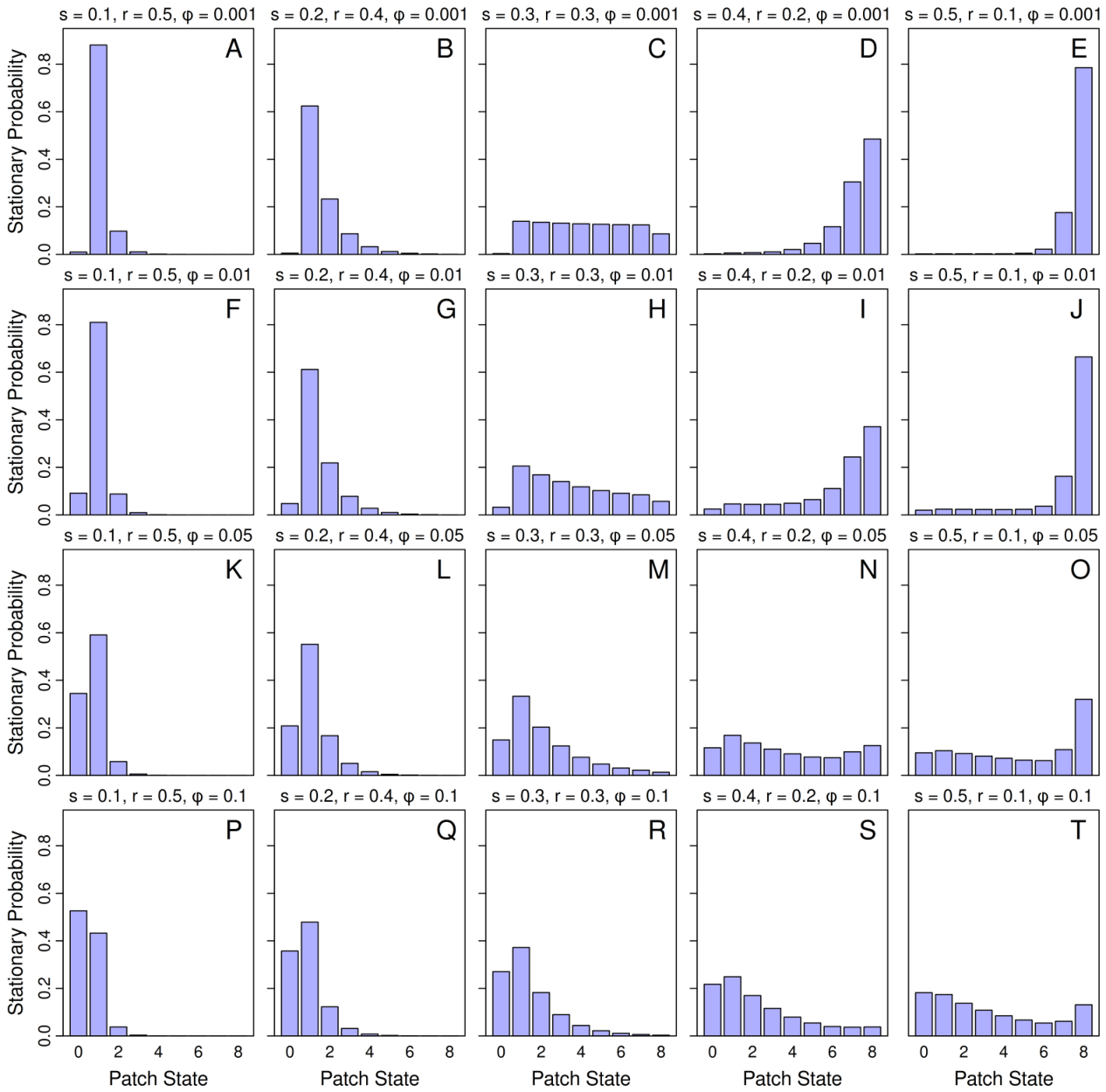
Here we provide two additional sets of examples of the stationary patch-type probability distribution like those of Figure 6 of the main text but with different orderings of succession, retrogression, and disturbance. The ordering in Figure 6 of the main text is . The ordering is in Figure A1 below and is in Figure A2.
Figure A1.
Stationary probability distributions of patch state for various choices of succession probability s, retrogression probability r, and disturbance probability under the constraints that and for all i. These examples are the same as in Figure 6 of the text (where ), except that retrogression occurs first, then succession, and then disturbance (). Note that reversing the order in which succession and retrogression act has not changed the qualitative patterns in the forms of the stable patch-state distribution.
Figure A1.
Stationary probability distributions of patch state for various choices of succession probability s, retrogression probability r, and disturbance probability under the constraints that and for all i. These examples are the same as in Figure 6 of the text (where ), except that retrogression occurs first, then succession, and then disturbance (). Note that reversing the order in which succession and retrogression act has not changed the qualitative patterns in the forms of the stable patch-state distribution.
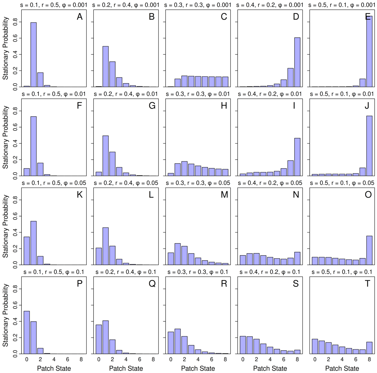
Figure A2.
Stationary probability distributions of patch state for various choices of succession probability s, retrogression probability r, and disturbance probability under the constraints that and for all i. These examples are the same as in Figure 6 of the text (where ), except that succession occurs first, then disturbance, and then retrogression (). Note that reversing the order in which retrogression and disturbance act has not changed the qualitative patterns in the forms of the stable patch-state distribution.
Figure A2.
Stationary probability distributions of patch state for various choices of succession probability s, retrogression probability r, and disturbance probability under the constraints that and for all i. These examples are the same as in Figure 6 of the text (where ), except that succession occurs first, then disturbance, and then retrogression (). Note that reversing the order in which retrogression and disturbance act has not changed the qualitative patterns in the forms of the stable patch-state distribution.
References
- Bott, T.L. Primary productivity and community respiration. In Methods in Stream Ecology, 2nd ed.; Hauer, F.R., Lamberti, G.A., Eds.; Elsevier: Amsterdam, The Netherlands, 2007; pp. 663–690. [Google Scholar]
- Çinlar, E. Introduction to Stochastic Processes; Dover Publications, Inc.: Mineola, New York, USA, 2013. [Google Scholar]
- Clements, F.E. Plant Succession: An Analysis of the Development of Vegetation, No. 242; Carnegie institution of Washington: Washington, D.C., USA, 1916. [Google Scholar]
- Connell, J.H. Diversity in tropical rain forests and coral reefs: high diversity of trees and corals is maintained only in a nonequilibrium state. Science 1978, 199, 1302–1310. [Google Scholar]
- Connell, J.H.; Slatyer, R.O. Mechanisms of succession in natural communities and their role in community stability and organization. Am. Nat. 1977, 111, 1119–1144. [Google Scholar] [CrossRef]
- Cooper, W.S. The climax forest of Isle Royale, Lake Superior, and its development. I. Botanical Gazette 1913, 55, 1–44. [Google Scholar] [CrossRef]
- DeAngelis, D.L.; Gross, L.J. (Eds.) Individual-Based Models and Approaches in Ecology: Populations, Communities, and Ecosystems; CRC Press: New York City, USA, 1992. [Google Scholar]
- DeNicola, D.M.; McNair, J.N.; Suh, J. A stochastic model of epilithic algal succession and patch dynamics in streams. Ecosphere 2021, 12, e03566. [Google Scholar] [CrossRef]
- Grace, M.; Imberger, S. Stream Metabolism: Performing and Interpreting Measurements; Water Studies Centre Monash University, Murray Darling Basin Commission and New South Wales Department of Environment and Climate Change: Victoria, Australia, 2006; Volume 204. [Google Scholar]
- Fisher, S.G.; Gray, L.J.; Grimm, N.B.; Busch, D.E. Temporal succession in a desert stream ecosystem following flash flooding. Ecol. Monogr. 1982, 52, 93–110. [Google Scholar] [CrossRef]
- Hanski, I. Metapopulation Ecology; Oxford University Press: New York City, USA, 1999. [Google Scholar]
- Hill, M.F.; Witman, J.D.; Caswell, H. Markov chain analysis of succession in a rocky subtidal community. Am. Nat. 2004, 164, E46–E61. [Google Scholar] [CrossRef]
- Horn, H.S. Markovian properties of forest succession. In Ecology and Evolution of Communities; Cody, M.L., Diamond, J.M., Eds.; Belknap Press of Harvard University Press: Cambridge, Massachusetts, USA, 1975; pp. 196–211. [Google Scholar]
- Horn, R.A.; Johnson, C.R. Matrix Analysis, 2nd ed; Cambridge University Press: New York City, USA, 2013. [Google Scholar]
- Khinchin, A.Y. Mathematical Foundations of Information Theory; Dover Publications, Inc.: Mineola, New York, USA, 1957. [Google Scholar]
- Lancaster, P.; Tismenetsky, M. The Theory of Matrices, 2nd ed.; Academic Press, Inc.: New York City, USA, 1985. [Google Scholar]
- Leibold, M.A.; Chase, J.M. Metacommunity Ecology; Princeton University Press: Princeton, New Jersey, USA, 2018. [Google Scholar]
- Levin, S.A.; Paine, R.T. Disturbance, patch formation, and community structure. Proc. Natl. Acad. Sci. 1974, 71, 2744–2747. [Google Scholar] [CrossRef]
- Lippe, E.; DeSmidt, J.T.; Glenn-Lewin, D.C. Markov models and succession: a test from a heathland in the Netherlands. J. Ecol. 1985, 73, 775–791. [Google Scholar] [CrossRef]
- McNair, J.N.; Zuidema, J.R. Stream community metabolism and dissolved-oxygen dynamics: where did the oxygen come from? Environ. 2025, 12, 236. [Google Scholar] [CrossRef]
- Paine, R.T.; Levin, S.A. Intertidal landscapes: disturbance and the dynamics of pattern. Ecol. Monogr. 1981, 51, 145–178. [Google Scholar] [CrossRef]
- R Core Team. R: A Language and Environment for Statistical Computing; R Foundation for Statistical Computing: Vienna, Austria, 2026. [Google Scholar]
- Randolph, A.D. A population balance for countable entities. Can. J. Chem. Eng. 1964, 42, 280–281. [Google Scholar] [CrossRef]
- Randolph, A.D.; Larson, M.A. Transient and steady state size distributions in continuous mixed suspension crystallizers. AIChE J. 1962, 8, 639–645. [Google Scholar] [CrossRef]
- Ricklefs, R.E. Ecology, 2nd ed.; Chiron Press, Inc.: New York City, USA, 1979. [Google Scholar]
- Runkle, J.R. Disturbance regimes in temperate forests. In The Ecology of Natural Disturbance and Patch Dynamics; Pickett, S.T.A., White, P.S., Eds.; Academic Press, Inc.: New York City, USA, 1985; pp. 17–33. [Google Scholar]
- Stephens, G.R.; Waggoner, P.E. The Forests Anticipated from 40 Years of Natural Transitions in Mixed Hardwoods. Bull. Connect. Agric. Exp. Stn. 1970, No. 707, 58 pages. [Google Scholar]
- Tanner, J.E.; Hughes, T.P.; Connell, J.H. Species coexistence, keystone species, and succession: a sensitivity analysis. Ecology 1994, 75, 2204–2219. [Google Scholar] [CrossRef]
- Usher, M.B. Markovian approaches to ecological succession. J. Anim. Ecol. 1979, 48, 413–426. [Google Scholar] [CrossRef]
- Waggoner, P.E.; Stephens, G.R. Transition probabilities for a forest. Nature 1970, 225, 1160–1161. [Google Scholar] [CrossRef]
- Watt, A.S. Pattern and process in the plant community. J. Ecol. 1947, 35, 1–22. [Google Scholar] [CrossRef]
- White, P.S.; Pickett, S.T.A. Natural disturbance and patch dynamics: an introduction. In The Ecology of Natural Disturbance and Patch Dynamics; Pickett, S.T.A., White, P.S., Eds.; Academic Press, Inc.: New York City, USA, 1985; pp. 3–13. [Google Scholar]
- Wilkinson, D.M. The disturbing history of intermediate disturbance. Oikos 1999, 84, 145–147. [Google Scholar] [CrossRef]
- Wootton, T.J. Prediction in complex communities: analysis of empirically derived Markov models. Ecology 2001, 82, 580–598. [Google Scholar] [CrossRef]
Figure 1.
Cooper’s idea that structural and functional properties at the community level remain approximately constant (top panel) because the continual changes occurring within different patches (bottom panels) balance each other. This concept is a fundamental part of the classical theory of patch dynamics and community structure.
Figure 1.
Cooper’s idea that structural and functional properties at the community level remain approximately constant (top panel) because the continual changes occurring within different patches (bottom panels) balance each other. This concept is a fundamental part of the classical theory of patch dynamics and community structure.
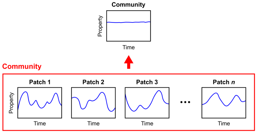
Figure 2.
The assumed hierarchy of habitats and patches, and of communities and subcommunities. Each habitat contains multiple patches. Each community contains multiple subcommunities, each of which occupies a single patch.
Figure 2.
The assumed hierarchy of habitats and patches, and of communities and subcommunities. Each habitat contains multiple patches. Each community contains multiple subcommunities, each of which occupies a single patch.
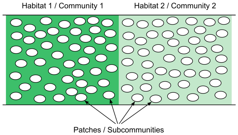
Figure 3.
The assumed sequence of succession, retrogression, and disturbance in the interval between consecutive observation times and . Succession occurs between observation time and notional time , retrogression between notional times and , and disturbance between and observation time .
Figure 3.
The assumed sequence of succession, retrogression, and disturbance in the interval between consecutive observation times and . Succession occurs between observation time and notional time , retrogression between notional times and , and disturbance between and observation time .
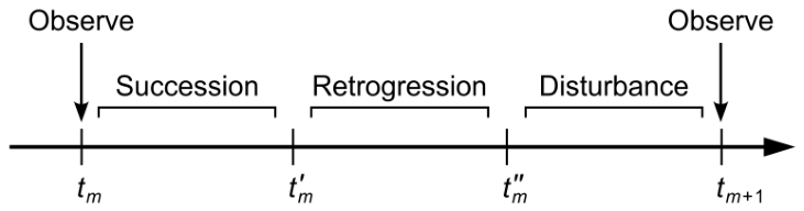
Figure 4.
Effects of succession, retrogression, and disturbance on patch states in a simple community comprising patches in a habitat. During the period between each pair of consecutive observation times and , succession acts first, then retrogression, and then disturbance. Each process acts independently on each patch. In this simple example, there are five possible patch states: 0, 1, 2, 3, and 4. Patches are labeled with their states at the end of each phase; arrows identify patches whose states changed during the current phase.
Figure 4.
Effects of succession, retrogression, and disturbance on patch states in a simple community comprising patches in a habitat. During the period between each pair of consecutive observation times and , succession acts first, then retrogression, and then disturbance. Each process acts independently on each patch. In this simple example, there are five possible patch states: 0, 1, 2, 3, and 4. Patches are labeled with their states at the end of each phase; arrows identify patches whose states changed during the current phase.
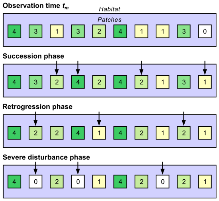
Figure 5.
Directed graphs for succession matrix , retrogression matrix , disturbance matrix , and matrix representing the combined effects of succession, retrogression, and disturbance.
Figure 5.
Directed graphs for succession matrix , retrogression matrix , disturbance matrix , and matrix representing the combined effects of succession, retrogression, and disturbance.
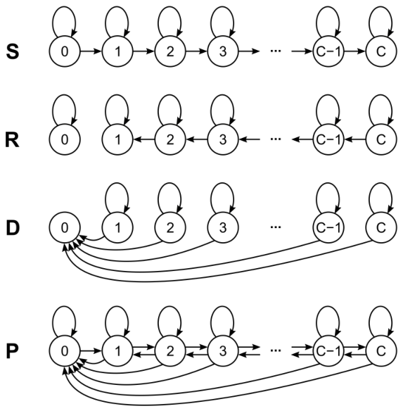
Figure 6.
Stationary patch-state probability distributions for various choices of succession probability s, retrogression probability r, and disturbance probability under the constraints that and for all i. There are 9 patch states. The disturbance probability is constant within each row of panels but increases from top to bottom rows. Succession and retrogression probabilities are constant within each column of panels, but succession probability increases and retrogression probability decreases from left to right columns. Retrogression is more prevalent than succession in column 1, succession is more prevalent than retrogression in column 5, and the two processes are balanced in column 3.
Figure 6.
Stationary patch-state probability distributions for various choices of succession probability s, retrogression probability r, and disturbance probability under the constraints that and for all i. There are 9 patch states. The disturbance probability is constant within each row of panels but increases from top to bottom rows. Succession and retrogression probabilities are constant within each column of panels, but succession probability increases and retrogression probability decreases from left to right columns. Retrogression is more prevalent than succession in column 1, succession is more prevalent than retrogression in column 5, and the two processes are balanced in column 3.
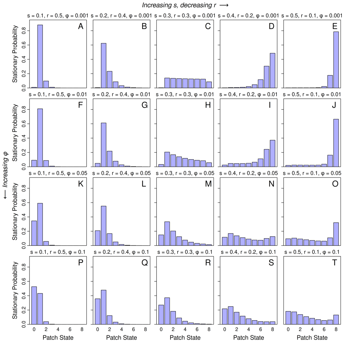
Figure 7.
Relationship between patch-state diversity H (vertical axis) and disturbance probability (horizontal axis) for five values of succession probability s. Values of retrogression probability r are the same as the s values but in reverse order, as in Table 1.
Figure 7.
Relationship between patch-state diversity H (vertical axis) and disturbance probability (horizontal axis) for five values of succession probability s. Values of retrogression probability r are the same as the s values but in reverse order, as in Table 1.
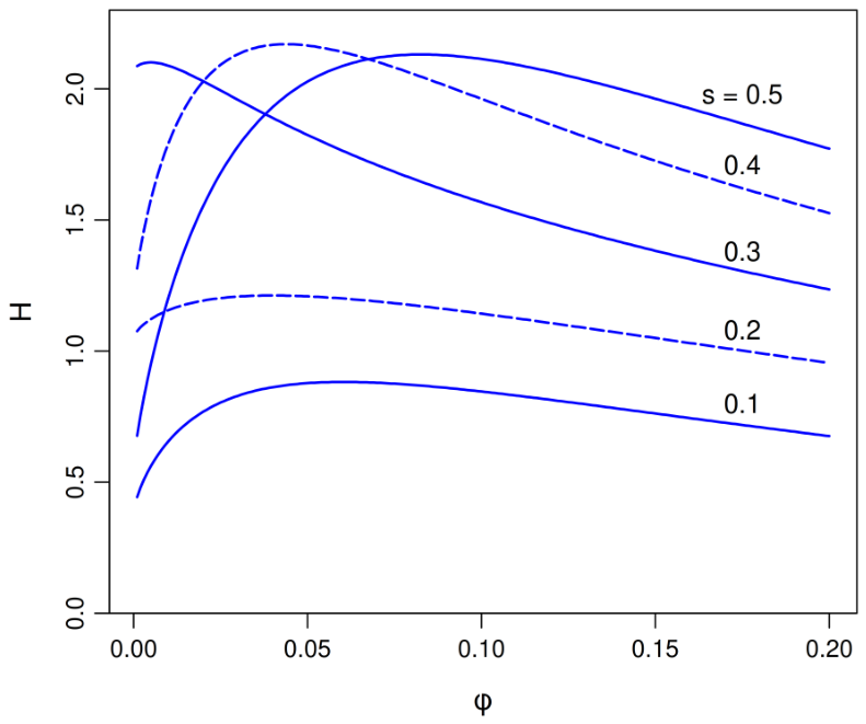
Figure 8.
Relationship between STEAS index (vertical axis) and the one-step probabilities of succession s (bottom horizontal axis) and retrogression r (top horizontal axis) for four values of disturbance probability . Open circles are the computed values of ; blue lines connecting the open circles are visual guides. The same values of hold for all possible orderings of succession, retrogression, and disturbance.
Figure 8.
Relationship between STEAS index (vertical axis) and the one-step probabilities of succession s (bottom horizontal axis) and retrogression r (top horizontal axis) for four values of disturbance probability . Open circles are the computed values of ; blue lines connecting the open circles are visual guides. The same values of hold for all possible orderings of succession, retrogression, and disturbance.
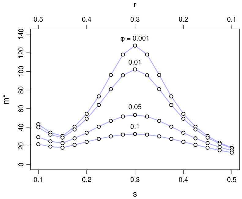
Figure 9.
Stacked bar plots showing the accelerated convergence of patch-state probability distribution to its stationary configuration as the probability of disturbance increases from (top panel) to (bottom panel). Succession and retrogression are balanced in all four cases. Segment heights within each bar represent patch-state probabilities for , with . Segment shading: patch state 0 is indicated by white, states 1 through 8 by increasingly darker shades of green.
Figure 9.
Stacked bar plots showing the accelerated convergence of patch-state probability distribution to its stationary configuration as the probability of disturbance increases from (top panel) to (bottom panel). Succession and retrogression are balanced in all four cases. Segment heights within each bar represent patch-state probabilities for , with . Segment shading: patch state 0 is indicated by white, states 1 through 8 by increasingly darker shades of green.
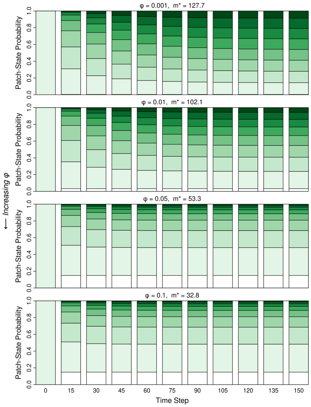
Figure 10.
Four types of patch boundaries. Top left: Patch boundaries (dashed lines) defined arbitrarily for sampling purposes and fixed in location for monitoring over time. Different individuals of the most conspicuous species are shown as small circles filled with black, white, or yellow to indicate different species. Patch types are defined by the most abundant species and are shaded white or different shades of green; white patches are disturbed. Example: [27]. Top right: Patch boundaries defined arbitrarily and fixed in location, with patches small enough so each contains at most one individual of the focal taxonomic group. Individuals of different species are shown as small circles filled with black, white, or yellow. Patch types are defined by the occupying species, as unoccupied but not disturbed, or as disturbed; white patches are disturbed. Example: [13]. Bottom left: Patches (ellipses) and their boundaries are physically real (e.g., stones in a stream bed). Patch types can be defined by various properties, such as taxonomic composition or physiognomy. Different shades of green indicate different types of undisturbed patches; white patches are disturbed. Example: [8]. Bottom right: Patches and their boundaries are physically real and were created by consecutive disturbance events, some of whose areas of impact overlap. Four patches are shown, labeled in order of creation. Patch age (time since creation) is indicated by shading, with older patches being darker green. The portion of each patch overlapped by a later patch becomes part of the later patch and acquires its age (initially zero). Dashed lines indicate parts of the original patch boundaries lost when disturbance events created overlapping patches. Example: We know of no model that employs this type of patch.
Figure 10.
Four types of patch boundaries. Top left: Patch boundaries (dashed lines) defined arbitrarily for sampling purposes and fixed in location for monitoring over time. Different individuals of the most conspicuous species are shown as small circles filled with black, white, or yellow to indicate different species. Patch types are defined by the most abundant species and are shaded white or different shades of green; white patches are disturbed. Example: [27]. Top right: Patch boundaries defined arbitrarily and fixed in location, with patches small enough so each contains at most one individual of the focal taxonomic group. Individuals of different species are shown as small circles filled with black, white, or yellow. Patch types are defined by the occupying species, as unoccupied but not disturbed, or as disturbed; white patches are disturbed. Example: [13]. Bottom left: Patches (ellipses) and their boundaries are physically real (e.g., stones in a stream bed). Patch types can be defined by various properties, such as taxonomic composition or physiognomy. Different shades of green indicate different types of undisturbed patches; white patches are disturbed. Example: [8]. Bottom right: Patches and their boundaries are physically real and were created by consecutive disturbance events, some of whose areas of impact overlap. Four patches are shown, labeled in order of creation. Patch age (time since creation) is indicated by shading, with older patches being darker green. The portion of each patch overlapped by a later patch becomes part of the later patch and acquires its age (initially zero). Dashed lines indicate parts of the original patch boundaries lost when disturbance events created overlapping patches. Example: We know of no model that employs this type of patch.
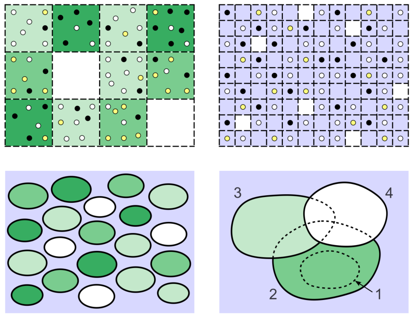

Table 1.
Dependence of patch-state diversity index H and STEAS index on one-step succession probability s, retrogression probability r, and disturbance probability in the numerical examples. Cases A–T correspond to those in Figure 6; additional cases were included to show the effect of a larger value of . For reference, the greatest lower bound for H is 0 and the least upper bound with nine patch states is .
Table 1.
Dependence of patch-state diversity index H and STEAS index on one-step succession probability s, retrogression probability r, and disturbance probability in the numerical examples. Cases A–T correspond to those in Figure 6; additional cases were included to show the effect of a larger value of . For reference, the greatest lower bound for H is 0 and the least upper bound with nine patch states is .
| Case | s | r | H | ||
|---|---|---|---|---|---|
| A | 0.1 | 0.5 | 0.001 | 0.443 | 43.298 |
| B | 0.2 | 0.4 | 0.001 | 1.076 | 54.471 |
| C | 0.3 | 0.3 | 0.001 | 2.087 | 127.701 |
| D | 0.4 | 0.2 | 0.001 | 1.315 | 54.471 |
| E | 0.5 | 0.1 | 0.001 | 0.677 | 18.061 |
| F | 0.1 | 0.5 | 0.010 | 0.656 | 39.902 |
| G | 0.2 | 0.4 | 0.010 | 1.156 | 49.204 |
| H | 0.3 | 0.3 | 0.010 | 2.088 | 102.083 |
| I | 0.4 | 0.2 | 0.010 | 1.792 | 49.204 |
| J | 0.5 | 0.1 | 0.010 | 1.204 | 17.441 |
| K | 0.1 | 0.5 | 0.050 | 0.878 | 29.397 |
| L | 0.2 | 0.4 | 0.050 | 1.209 | 34.154 |
| M | 0.3 | 0.3 | 0.050 | 1.824 | 53.328 |
| N | 0.4 | 0.2 | 0.050 | 2.165 | 34.154 |
| O | 0.5 | 0.1 | 0.050 | 2.028 | 15.085 |
| P | 0.1 | 0.5 | 0.100 | 0.846 | 21.854 |
| Q | 0.2 | 0.4 | 0.100 | 1.143 | 24.378 |
| R | 0.3 | 0.3 | 0.100 | 1.568 | 32.795 |
| S | 0.4 | 0.2 | 0.100 | 1.962 | 24.378 |
| T | 0.5 | 0.1 | 0.100 | 2.114 | 12.815 |
| – | 0.1 | 0.5 | 0.150 | 0.762 | 17.191 |
| – | 0.2 | 0.4 | 0.150 | 1.050 | 18.715 |
| – | 0.3 | 0.3 | 0.150 | 1.382 | 23.308 |
| – | 0.4 | 0.2 | 0.150 | 1.726 | 18.715 |
| – | 0.5 | 0.1 | 0.150 | 1.962 | 11.057 |
Disclaimer/Publisher’s Note: The statements, opinions and data contained in all publications are solely those of the individual author(s) and contributor(s) and not of MDPI and/or the editor(s). MDPI and/or the editor(s) disclaim responsibility for any injury to people or property resulting from any ideas, methods, instructions or products referred to in the content. |
© 2026 by the authors. Licensee MDPI, Basel, Switzerland. This article is an open access article distributed under the terms and conditions of the Creative Commons Attribution (CC BY) license (http://creativecommons.org/licenses/by/4.0/).
Copyright: This open access article is published under a Creative Commons CC BY 4.0 license, which permit the free download, distribution, and reuse, provided that the author and preprint are cited in any reuse.