

Submitted:
03 November 2026
Posted:
05 November 2026
You are already at the latest version
Abstract
The paper is devoted to the study of the tissue optical clearing effect through numerical experiment on the reconstruction of a phantom with a fluorophore with the use of mesoscopic fluorescence molecular tomography (MFMT). This is the first attempt to answer the question of whether it is possible to improve the accuracy of reconstructing spatial structures and the sensitivity of MFMT to the structure reproduction depth by optically clearing the superficial tissue layers. The reconstruction region is a cube 10x10x10 mm3 in size. The fluorophore is specified as two nested cylindrical shells 1 mm thick at a distance of 1 mm between them. This allows us to estimate the modulation transfer coefficient for structures 1 mm in size for the entire depth of the object. Fluorescence signals and spatial sensitivity functions are modeled in reflectance geometry by the Monte Carlo method with the TurbidMC code. The inverse problem is solved using the algebraic reconstruction technique with fast iterative shrinkage thresholding and total variation regularization. Reconstruction results and their quantitative analysis using the modulation transfer coefficient show that optical clearing makes it possible to increase the depth at which fluorescent structures can be accurately reproduced—from 5.5 to 9 mm.
Keywords:
mesoscopic fluorescence molecular tomography (MFMT)
; optical clearing
; TurbidMC
; spatial sensitivity function (SSF)
; reconstruction algorithm
; modulation transfer coefficient
; depth sensitivity
1. Introduction
In the last two decades, fluorescence molecular tomography (FMT) [1,2,3] is widely used as a molecular imaging method for solving problems in experimental oncology such as the elucidation of mechanisms of carcinogenesis, the study of the pharmacokinetics of potential drugs, and the selection of strategies for the treatment of various tumors. Unlike 2D fluorescence microscopy [4], FMT reconstructs and visualizes the 3D spatial distributions of fluorescent targets inside a small animal volume. However, due to multiple scattering of photons in deep tissues, the spatial resolution of macroscopic FMT is strongly limited. Many approaches have been proposed to improve FMT resolution, including the use of early arriving photons [5,6], optimization of illumination patterns [7,8], a large number of FMT measurements [9,10], and improved reconstruction algorithms such as the compressed sensing based ones [11,12,13]. But it has appeared that perhaps the most effective way to improve spatial resolution is to change from the macroscopic mode of data acquisition to the mesoscopic one that utilizes very small source-detector distances (SDDs) (from zero to a few millimeters). The mesoscopic FMT (MFMT) method helps attain submillimeter spatial resolution (80-100 μm) [14] and is successfully practiced by many researchers [14,15,16,17]. Unfortunately, small (compared to the macroscopic mode) SDDs inevitably make the reconstruction region smaller in size and worsen the depth sensitivity of FMT. Thus the researchers have a new problem before them: develop a method that could help increase the depth available for the accurate reproduction of fluorescent structures in MFMT.
From the first steps in the development of diffuse optical spectroscopy (or near-infrared spectroscopy) [18], the notion of the depth sensitivity has intimately been associated with the spatial sensitivity function (SSF). The function was first introduced by Feng et al. [19]; it defines the weight contribution of each point (voxel) of an object to the signal registered by the detector from the source and in the case of reflectance geometry its shape resembles a banana. Feng et al. [19] derived analytical expressions for SSF in case of continuous-wave (CW) measurements and proposed that the depth sensitivity was characterized by the maximal depth of SSF penetration to the interior of the scattering object. Del Bianco et al. [20] and Gunadi et al. [21] use the average penetration depth of SSF. Diop et al. [22] and Milej et al. [23] showed that the depth sensitivity could be increased by changing from CW measurements to time-domain ones and registering not intensity, but times-of-flight of diffusive photons and variances of times-of-flight. Another approach presented by Milej et al. [24,25] is to apply a subtraction method to high order statistical moments of times-of-flight measured at two SDDs. The recent paper by Blaney et al. [26] is an excellent overview that traces the 30-year history of works investigating the spatial sensitivity for various diffuse optical spectroscopy methods and data types. But despite that huge number of publications, the further increase of the depth sensitivity is still the topic of the day.
Currently, a highly effective alternative to established FMT methods is a new approach that utilizes tissue optical clearing, based on impregnating tissues with biocompatible agents that are widely used in medical practice [27,28,29,30,31,32]. Tissue optical clearing methods are employed to reduce the light-scattering properties of tissues, thereby increasing the depth of light penetration. Various optical clearing agents—such as glucose, propylene glycol, glycerol, and polyethylene glycol, among others—are used effectively for in vitro, ex vivo, and in vivo studies [27]. Recently Tuchina et al. [33] and Jaafar et al. [34] has demonstrated that contrast agents used in magnetic resonance imaging (such as Gadovist, Magnevist, and Dotarem), as well as the X-ray contrast agent Visipaque, provide a relatively stable clearing effect within the superficial tissue layer. Specifically, study [33] experimentally confirmed that these substances can reduce the scattering coefficient by half within a 1 mm-thick superficial tissue layer. The clearing effect persists for tens of minutes, which is more than sufficient for conducting a series of measurements using the MFMT method.
In Ref. [35], the authors employed this specific mathematical model of tissue optical clearing to calculate SSFs using the Monte Carlo method. It was demonstrated that, with a source-detector distance SDD of 5 mm, optical clearing of the surface layer increased the maximum penetration depth of SSF from ~5 mm to ~7 mm. Based on this result, the authors hypothesized that optical clearing could effectively enhance sensitivity to the depth of embedded objects—not only in diffuse optical spectroscopy but also in MFMT. Naturally, the criterion for assessing sensitivity in MFMT—where SDD values vary across a relatively wide range—differs from the criterion used in diffuse optical spectroscopy. As noted above, to validate this hypothesis, it is necessary to reconstruct fluorescence tomograms and determine the limiting depth at which fluorescent structures can still be visualized with acceptable quality. This is precisely the task addressed and resolved in the present paper.
The paper is organized as follows. Section 2 briefly describes methods and means that are used to model fluorescence signals and SSFs, and to solve the inverse problem of MFMT. It also describes data acquisition geometry and numerical phantoms used in the study. Section 3 presents results of numerical experiment, including the calculated fluorescence signals and SSFs, reconstructed fluorescent tomograms, and estimates for the reconstruction accuracy of fluorescent structures at different depths, which are obtained with the help of the modulation transfer coefficient analysis. Section 4 provides inferences and directions of further research.
2. Methods
2.1. General Remarks
The FMT method is unique in its potential for the reconstruction of spatial distributions for not only the fluorophore concentration (or the fluorophore absorption coefficient), but also for the fluorescence lifetime – a parameter that is of great importance for solving the problems of experimental oncology [36]. In recent years, the authors of this paper have developed an original time-domain FMT method [6,35,37,38,39] that is based on the asymptotic approximation to the fluorescence source function and allows separation of fluorophore absorption coefficient and fluorescence lifetime distributions directly in the time domain. In Refs. [6,37], the method is investigated in numerical experiment; Refs. [35,38] describe two physical experiments with phantoms; and, finally, in Ref. [39], the results obtained by the authors are thoroughly analyzed and found encouraging. However in this work, to avoid possible errors, specifically, in the separation of fluorescence parameters, we decided to reduce the reconstruction problem to its lowest terms and consider the case of continuous-wave FMT (CW-FMT) with recovering the distributions of the fluorophore absorption coefficient only. In addition, for the simulation of fluorescence signals and SSFs by the Monte Carlo method, we use complete a priori knowledge on the fluorophore location in the phantom, the fluorescence parameters, and the phantom’s optical parameters. This is done with the purpose of getting a “maximum” estimate for the ultimate depth at which it is still possible to reconstruct the fluorescent structures accurately. It must be understood here that this depth may appear unattainable in the real physical experiment.
2.2. Forward Model and Inverse Problem
In macroscopic FMT, the forward problem (i.e., light propagation through a scattering object) is generally solved using the diffusion approximation to the radiative transfer equation [2]. But in the case of the mesoscopic mode, such a forward model does not suit due to the limited volume interrogation and anisotropic light propagation [40]. That is why in this work we model fluorescence signals and SSFs with the TurbidMC code [35,41] that implements the perturbation Monte Carlo method. The code was developed by the authors of this paper especially for solving the forward problem of time-domain MFMT. Of course, it can be used in the CW case as well. A detailed description of the algorithm implemented in TurbidMC can be found in Ref. [41], and some its modifications we implemented later to make calculations faster and to improve calculation statistics are described in Ref. [35]. In this paper, the modified version of the code is used. For calculations we use the assumption that the optical parameters of the phantom at the excitation and emission wavelengths are equal each other. This assumption is standard for FMT when the therapeutic transparency window is meant [42]. Then the procedure of SSF calculations is simplified and the sensitivity functions for fluorescence can be simulated as the sensitivity functions for absorption perturbations [42]. All TurbidMC calculations were performed on a multiprocessor cluster of Russian Federal Nuclear Center – Zababakhin All-Russia Research Institute of Technical Physics (Snezhinsk, Russia).
The inverse problem of CW-FMT is reduced to the solution of the Fredholm linear integral equation of the first kind (see, for example, [17])
where p(rs,rd) is the fluorescence signal (intensity) excited by source at point rs and recorded by detector at point rd, k is the dimensionless proportionality coefficient, V is the volume of the region of interest (ROI), W(rs,rd,r) is SSF calculated by TurbidMC for a given source-detector (SD) link, and μaf(r) is the sought distribution of the fluorophore absorption coefficient. Discretization of equation (1) with M SD links and N voxels of ROI gives the system of linear algebraic equations
where W ∈ RM×N is the sensitivity matrix, which contains discrete transposed SSFs calculated for all SD links involved in reconstruction, μ ∈ RN×1 is the vector describing the sought distribution μaf(r), and p is the vector of measurement data. Because in our case system (2) is strongly underdetermined (see subsection 2.2), one of the optimization algorithms with regularization should be used to solve it. In this paper, the compressed sensing based algorithm ART-FIST-TV (algebraic reconstruction technique (ART) with fast iterative shrinkage thresholding (FIST) and total variation (TV) regularization) [38] was chosen to solve (2). This algorithm firstly performs a cycle of ART iterations, and then the shrinkage-thresholding operator is applied as it is described in Ref. [43]. After a cycle of ART-FIST iterations a cycle of TV iterations with the steepest descent method [44,45] is implemented. Then an external cycle is organized where these two internal cycles work one after another. Our reconstruction framework was implemented with the MATLAB package. All calculations with it were performed on an Intel PC with a 3.4 GHz i5 processor and 8 GB RAM.
Wμ = p,
2.3. Geometry and Phantoms
For their numerical experiment the authors chose the reflectance geometry that is traditional in MFMT [14,15,16,17,35,38]. The phantom is a scattering object of size 10x10x10 mm3 (ROI). Sources are arranged on one of its faces. They also act as detectors. The fluorophore is formed by two nested cylindrical shells. The shells are 1 mm thick and 9 mm long, the distance between them is also 1 mm. So, they form the periodical spatial structures of 1 mm in size in the radial directions. This allows us to estimate the modulation transfer coefficient from the images we reconstruct for the 1-mm-structures through the entire phantom depth. The phantom with the fluorophore is shown in Figure 1. The blue dots mark the position of 121 sources and, accordingly, 121 detectors.
TurbidMC calculations and further reconstructions were done for two versions of the phantom. In the first case, the optical parameters remained constant in the entire phantom volume. In the second case, the phantom had a cleared surface layer 1mm in thickness where the scattering coefficient was 2 times lower than in the phantom. The optical parameters of the phantom before and after clearing are adapted from Ref. [46] and provided in Table 1. The fluorescence parameters used in calculations correspond to the fluorescent protein TagRFP [35] and are presented in Table 2. Since the excitation and emission wavelengths of this fluorophore are very close, the same values of the optical and fluorescence parameters were used for both wavelengths.
Figure 2 demonstrates how the SD links are formed. The source is first put at the point (0, 0, 0). All links for the source are shown in Figure 2(a). Let us refer to the SD links for which SSFs should necessarily be calculated as “unique”. They are 19 (shown in green). Accordingly, the “non-unique” links (shown in grey) are the links for which the sensitivity functions can be determined from calculations for the unique SD links. Then the source with all its links formed is moved to a neighbor point, for example, with coordinates (1 mm, 1 mm, 0) (Figure 2(b)). The red dashed lines in Figure 2(b) show the links that go beyond the square 10×10 mm2. These links are removed from consideration. Only the working links (green lines) remain and they are added to the SD links of Figure 2(a). Then the links of Figure 2(а) are moved to the next position and thus all source positions shown in Figure 1(b) are searched. The total number of SD links involved in reconstruction is M=8160.
The reconstruction region (ROI) was divided into 100×100×100 voxels, i.e., N=1000000. The size of the sensitivity matrix, 8160×1000000, suggests that system (2) is strongly underdetermined and it is necessary to apply a reconstruction algorithm with regularization (ART-FIST-TV in our case).
3. Results and Their Analysis
3.1. Fluorescence Signals and SSFs
In TurbidMC calculations, each source and each detector were defined by a 100-μm-diam circle on the XOY plane. The source uniformly emits the exciting photons into the phantom and the detector receives the fluorescence photons at an aperture (critical) angle below 8.2 degrees. This model corresponds to the conditions of a real physical experiment where the light is input and output through a 100-μm-diam optic fiber with numerical aperture 0.2. About 109 histories were tracked in each of the calculations. Each history started with the entry of the photon in the phantom and tracked all the trajectories it formed. The fluorescence signal was calculated as the intensity of all fluorescence photons that reached the detector (i.e., crossed the detector circle in the aperture angle cone) per an exciting photon. The fluorescence signals normalized to the coefficient k (see formula (1)) are plotted in Figure 3. The plot of Figure 3(a) presents the signals simulated for the SD links of Figure 2(a), and that of Figure 3(b) is for the signals simulated for the links of Figure 2(b).
SSF for each unique SD link was calculated as a 3D spatial distribution of weight contributions to the signal from each voxel in ROI. The sensitivity functions for the non-unique SD links were obtained from the results for the unique ones by the spatial transformations. As an example Figure 4 visualizes the results obtained in the simulation of SSFs for SDD of 4 mm. It shows not the 3D distributions but their 2D sections in the XOZ plane as bearing the most illustrative information. Figure 4(a) shows the result for the non-cleared phantom, and Figure 4(b), for the phantom with the cleared surface layer. To help easily evaluate by eye the maximal depth of SSF penetration, the intensity of each pixel in the SSF section was raised to the 5/2 power (chosen empirically). The comparison of two SSFs in Figure 4 clearly shows that in the case of clearing (Figure 4(b)), SSF penetrates much deeper into the phantom and the gain in the maximum penetration depth is about 1.5- 2 mm. This result agrees well with that one reported in [35].
For the selected parameters, the time of one fluorescence signal calculation was equal to ~30 minutes, and the time of one SSF calculation reached several hours on the multiprocessor cluster.
3.2. Reconstruction Results
As stated in subsection 2.2, the images of the phantoms with and without optical clearing were reconstructed with the ART-FIST-TV algorithm. The numbers of iterations in the inner and external cycles which are now hyper-parameters were chosen empirically. The best results were obtained where the number of iterations in the ART-FIST cycle was 10, the number of iterations in the TV cycle was 1, and the number of external iterations was 200. The total reconstruction time was 19-20 hours.
Figure 5 and Figure 6 present the best tomograms the authors obtained in the reconstruction of the fluorophore absorption coefficient distributions for phantoms without and with optical clearing. Figure 5 shows the frontal sections of the 3D reconstructions in comparison with the frontal section of the phantom. Figure 6 presents the cross-sections of the 3D images in the planes z = 3 mm; z = 5 mm; and z = 7 mm. All reconstruction results are presented without colorbars. In all cases, the MATLAB’s palette PARULA with a minimal value equal to zero and a maximal value equal to 0.17 mm-1 is used for visualization. The visual analysis of Figure 5 and Figure 6 suggests that at depths from 5 mm and on, the reproduction of the fluorescent shells in the phantom with clearing is much better than in the phantom with no clearing. This is seen from the loss of many shell parts at depths above 5 mm in the phantom without clearing, while in the phantom with clearing the shell structure is well seen down to depths about 8.5-9 mm. To confirm the visual effect quantitatively, we have analyzed the images using the modulation transfer coefficient [47] and Foucault-Rayleigh criterion [48].
3.3. Modulation Transfer Coefficient Analysis
The modulation transfer function analysis [47] is known to be the best way to reliably control the accuracy of structure reproduction by evaluating the spatial resolution. In order to construct the modulation transfer function, it is necessary to consider a phantom with rows of periodic spatial structures. For each row with structures of one size, the modulation transfer coefficient can be estimated as a mean relative dip between two maxima. The modulation transfer function is the dependence of the modulation transfer coefficient on spatial frequency. The resolution is determined from the Foucault-Rayleigh criterion [48]: the structures are resolved relative to each other if the modulation transfer coefficient is greater than or equal to 20%. In diffusion tomography, this approach was used, for example, in Refs. [49,50,51,52].
In the phantom of Figure 1, the fluorescent shells also form a periodic structure, whose size is defined by their thickness (1 mm). Therefore, we can estimate the modulation transfer coefficient for structures 1 mm in size for the entire range depths in the phantom in any radial direction. Figure 7 illustrates the scheme of this estimation. Cross-sections of 3D images reconstructed (one of them is shown in Figure 7(a)) were visualized for various depths taken with at a step of 0.1 mm. For each cross-section, 8 radial directions (red arrows in Figure 7(a)) were chosen to construct 8 profiles (the entire family of profiles is shown in Figure 7(b)). The modulation transfer coefficient was determined from each profile as the relative dip between two maxima. For a sample of 8 values resulted, the mean value and root-mean-square deviations were calculated. These data obtained for all depths are visualized in Figure 8 as the dependencies of the modulation transfer coefficient on depth for the non-cleared and cleared phantoms.
It is seen rom Figure 8 that the red line corresponding to the 20% contrast intersects the broadened (due to the visualization of error bars) green line at depths within (5.4 mm, 5.8 mm), and the broadened blue line, at depths within (9.1 mm, 9.8 mm). So, optical clearing allows the gain in the depth at which the fluorescent structures are still reproduced with acceptable accuracy to reach no smaller than 3.3 mm. This outcome should undoubtedly be deemed as positive. On the level of numerical experiment on the reconstruction of fluorescent tomograms, it confirms the hypothesis propounded in [35]: the optical clearing of tissue may significantly improve the depth sensitivity of the MFMT method which is of utmost importance in the case of the mesoscopic data acquisition mode.
4. Discussion and Conclusions
Today the optical clearing methods are widely applied by researches to improve the image quality of various optical imaging modalities. They include optical coherence tomography, laser speckle contrast imaging, Raman microscopy, multiphoton microscopy, light sheet fluorescence microscopy, photoacoustic imaging, and so on [27,28,29,30,31,32,33,34]. At present, fluorescence molecular tomography remains poorly explored in this context. One likely reason is that, in macroscopic fluorescence tomography, the penetration depth of diffuse light into tissue is quite significant (up to several centimeters), rendering it unnecessary to alter the tissue’s optical properties to increase the probing depth. Nevertheless, even in this scenario, optical clearing of the superficial tissue layers can be highly beneficial for detecting weak fluorescence signals originating from individual cancer cells [33]. But the situation has drastically changed due to the development of laminar optical tomography and mesoscopic fluorescence tomography methods practicing the mesoscopic data acquisition mode. In this context, the task the authors of the paper imposed, specifically, to study the efficiency of tissue optical clearing as applied to such a method as mesoscopic fluorescence molecular tomography is expressly relevant. The results we obtained seem to surpass all imagination. We succeeded to show numerically that the gain the optical clearing of a 1-mm-thick surface layer gives in the depth at which the fluorescent structures on the tomographic images are still reproduced with acceptable accuracy reaches 3 mm and even more. Such a great result could hardly be expected because our earlier calculations showed that the gain in the depth of the spatial sensitivity function penetration into a scattering object was no higher than 1.5 -2 mm.
It should be noted that our numerical study was done with a number of simplifying restrictions which makes it necessary for us to state that the estimate we obtained for the probing depth is a “maximum” estimate. Firstly, in the simulation of fluorescence signals and calculation of spatial sensitivity functions, we used full a priori information on fluorophore position and configuration, and on the optical parameters of the phantom and fluorescence parameters. Secondly, we considered rather a simple case of continuous-wave fluorescence tomography that does not allow visualization of fluorescence lifetime – a very important parameter for studies in experimental oncology. Thirdly, the phantom with the fluorophore we took for our study is very far from reality. It allows us to solve a particular local problem – to assess the reproduction depth of a fluorescent structure 1 mm in size. This value is at least 10 times larger than the limit of spatial resolution in mesoscopic fluorescence tomography. That is why we have no ground to claim that the smaller high-frequency structures can be reproduced with the same depth sensitivity. This again confirms the fact that our estimate for the ultimate probing depth is a “maximum” estimate.
Despite however all the above limitations, our results indicate that the problem stated in this paper is solved: we have proved that optical clearing can and, perhaps, must be applied in mesoscopic fluorescence molecular tomography as a way to increase the depth sensitivity of the method. In this aspect this work is innovative. We very much hope that it will be followed by other publications. In the future we plan to return to our time-domain mesoscopic fluorescence molecular lifetime tomography based on the asymptotic approximation to the fluorescence source function and demonstrate the capabilities optical clearing offers for the reconstruction of fluorescence lifetime distributions. Our future plan also includes a physical experiment on the reconstruction of a more realistic phantom with fluorophore and in vivo mice experiments.
We are also encouraged by the fact that experimental data for dermis treated with glycerol show a significant increase in the scattering anisotropy factor g—from approximately 0.7 to 0.99 [53]—which could substantially affect the efficiency of fluorescence image reconstruction (given that a maximum value of 0.95 was used in our calculations).
Author Contributions
Conceptualization, A.B.K and V.V.T.; methodology, A.B.K. and V.V.V.; investigation, A.B.K., V.V.V., S.I.S., I.D.S. and D.K.T.; software, V.V.V. and S.I.S.; writing – original draft preparation, A.B.K. and V.V.V.; writing – review and editing, A.B.K., A.P.S., O.P.C. and V.V.T.; project administration, A.P.S., O.P.C. and V.V.T.; funding acquisition, A.P.S., O.P.C. and V.V.T. All authors have read and agreed to the published version of the manuscript.
Funding
The investigation was supported by the Russian Science Foundation with Grant No. 26-63-00028. https://rscf.ru/en/project/26-63-00028/.
Data Availability Statement
The data are available from the authors.
Conflicts of Interest
The authors declare no conflicts of interest.
Abbreviations
The following abbreviations are used in this manuscript:
| MFMT | Mesoscopic fluorescence molecular tomography |
| FMT | Fluorescence molecular tomography |
| SSF | Spatial sensitivity function |
| SDD | Source-detector distance |
| CW | Continuous-wave |
| CW-FMT | Continuous-wave fluorescence molecular tomography |
| ROI | Region of interest |
| SD | Source-detector |
| ART-FIST-TV | Algebraic reconstruction technique with fast iterative shrinkage thresholding and total variation regularization |
| ART | Algebraic reconstruction technique |
| FIST | Fast iterative shrinkage thresholding |
| TV | Total variation |
References
- Stuker, F.; Ripoll, J.; Rudin, M. Fluorescence molecular tomography: Principles and potential for pharmaceutical research. Pharmaceutics 2011, 3, 229–274. [Google Scholar] [CrossRef] [PubMed]
- Darne, C.; Sevick-Muraca, E.M. Small animal fluorescence and bioluminescence tomography: a review of approaches, algorithms and technology update. Phys. Med. Biol. 2014, 59, R1–R64. [Google Scholar] [CrossRef] [PubMed]
- An, Y.; Wang, K.; Tian, J. Recent methodology advances in fluorescence molecular tomography. Vis. Comput. Ind. Biomed. Art. 2018, 1, 1. [Google Scholar] [CrossRef]
- Stockert, J.C.; Blazquez-Castro, A. Fluorescence Microscopy in Life Science; Bentham Science: Sharjah, United Arab Emirates, 2017. [Google Scholar]
- Zhang, B.; Cao, X.; Liu, F.; Liu, X.; Wang, X.; Bai, J. Early-photon fluorescence tomography of a heterogeneous mouse model with the telegraph equation. Appl. Opt. 2011, 50, 5297–5407. [Google Scholar] [CrossRef] [PubMed]
- Konovalov, A.B.; Vlasov, V.V.; Uglov, A.S. Early-photon reflectance fluorescence molecular tomography for small animal imaging: Mathematical model and numerical experiment. Int. J. Numer. Meth. Biomed. Eng. 2021, 37, e3408. [Google Scholar] [CrossRef] [PubMed]
- Dutta, J.; Ahn, S.; Joshi, A.A.; Leahy, R.M. Illumination pattern optimization for fluorescence tomography: theory and simulation studies. Phys. Med. Biol. 2010, 55, 2961–2982. [Google Scholar] [CrossRef] [PubMed]
- Ducros, N.; D’Andrea, C.; Bassi, A.; Valentini, G.; Arridge, S. A virtual source pattern method for fluorescence tomography with structured light. Phys. Med. Biol. 2012, 57, 3811–3832. [Google Scholar] [CrossRef] [PubMed]
- Lee, J.H.; Kim, H.K.; Chandhanayingyong, C.; Lee, F.Y.-I.; Hielscher, A.H. Non-contact small animal fluorescence imaging system for simultaneous multi-directional angular-dependent data acquisition. Biomed. Opt. Express 2014, 5, 2301–2316. [Google Scholar] [CrossRef] [PubMed]
- Wang, D.; He, J.; Qiao, H.; Li, P.; Fan, Y.; Li, D. Noncontact full-angle fluorescence molecular tomography system based on rotary mirrors. Appl. Opt. 2015, 54, 7062–7070. [Google Scholar] [CrossRef] [PubMed]
- Dutta, J.; Ahn, S.; Li, C.; Cherry, S.R.; Leahy, R.M. Joint L1 and total variation regularization for fluorescence molecular tomography. Phys. Med. Biol. 2012, 57, 1459–1476. [Google Scholar] [CrossRef] [PubMed]
- Jiang, S.; Liu, J.; An, Y.; Zhang, G.; Ye, J.; Mao, Y.; He, K.; Chi, C.; Tian, J. Novel L2,1-norm optimization method for fluorescence molecular tomography reconstruction. Biomed. Opt. Express 2016, 7, 2342–2359. [Google Scholar] [CrossRef] [PubMed]
- Yuan, Y.; Yi, H.; Kang, D.; Yu, J.; Guo, H.; He, X.; He, X. Robust transformed L1 metric for fluorescence molecular tomography. Comput. Meth. Programs Biomed. 2023, 234, 107503. [Google Scholar] [CrossRef] [PubMed]
- Yang, F.; Ozturk, M.S.; Zhao, L.; Cong, W.; Wang, G.; Intes, X. High-resolution mesoscopic fluorescence molecular tomography based on compressed sensing. IEEE Trans. Biomed. Eng. 2015, 62, 248–255. [Google Scholar] [CrossRef] [PubMed]
- Azimipour, M.; Sheikhzadeh, M.; Baumgartner, R.; Cullen, P.K.; Helmstetter, F.J.; Chang, W.-J.; Pashaie, R. Fluorescence laminar optical tomography for brain imaging: system implementation and performance evaluation. J. Biomed. Opt. 2017, 22, 016003. [Google Scholar] [CrossRef]
- Tang, Q.; Liu, Y.; Tsytsarev, V.; Lin, J.; Wang, B.; Kanniyappan, U.; Li, Z.; Chen, Y. High-dynamic-range fluorescence laminar optical tomography (HDR-FLOT). Biomed. Opt. Express 2017, 8, 2124–2137. [Google Scholar] [CrossRef] [PubMed]
- Yang, F.; Gong, X.; Faulkner, D.; Gao, S.; Yao, R.; Zhang, Y.; Intes, X. Accelerating vasculature imaging in tumor using mesoscopic fluorescence molecular tomography via a hybrid reconstruction strategy. Biochem. Biophys. Res. Commun. 2021, 562, 29–35. [Google Scholar] [CrossRef] [PubMed]
- Ozaki, Y.; Huck, C.; Tsuchikawa, S.; Engelsen, S.B. (Eds.) Near-Infrared Spectroscopy: Theory, Spectral Analysis, Instrumentation, and Applications; Springer Nature Singapore Pte Ltd.: Gateway East, Singapore, 2021. [Google Scholar] [CrossRef]
- Feng, S.; Zeng, F.-A.; Chance, B. Photon migration in the presence of a single defect: a perturbation analysis. Appl. Opt. 1995, 34, 3826–3837. [Google Scholar] [CrossRef] [PubMed]
- Del Bianco, S.; Martelli, F.; Zaccanti, G. Penetration depth of light re-emitted by a diffusive medium: Theoretical and experimental investigation. Phys. Med. Biol. 2002, 47, 4131–4144. [Google Scholar] [CrossRef] [PubMed]
- Gunadi, S.; Leung, T.S.; Elwell, C.E.; Tachtsidis, I. Spatial sensitivity and penetration depth of three cerebral oxygenation monitors. Biomed. Opt. Express 2014, 5, 2896–2912. [Google Scholar] [CrossRef] [PubMed]
- Diop, M.; St Lawrence, K. Improving the depth sensitivity of time-resolved measurements by extracting the distribution of times-of-flight. Biomed. Opt. Express 2013, 4 doi, 447–459. [Google Scholar]
- Milej, D.; Janusek, D.; Gerega, A.; Wojtkiewicz, S.; Sawosz, P.; Treszczanowicz, J.; Weigl, W.; Liebert, A. Optimization of the method for assessment of brain perfusion in humans using contrast-enhanced reflectometry: multidistance time-resolved measurements. J. Biomed. Opt. 2015, 20, 106013. [Google Scholar] [CrossRef] [PubMed]
- Milej, D.; Abdalmalak, A.; Janusek, D.; Diop, M.; Liebert, A.; St Lawrence, K. Time-resolved subtraction method for measuring optical properties of turbid media. Appl. Opt. 2016, 55, 1507–1513. [Google Scholar] [CrossRef] [PubMed]
- Milej, D.; Abdalmalak, A.; McLachlan, P.; Diop, M.; Liebert, A.; St Lawrence. Subtraction-based approach for enhancing the depth sensitivity of time-resolved NIRS. Biomed. Opt. Express 2016, 7, 4514–4526. [Google Scholar] [CrossRef] [PubMed]
- Blaney, G.; Sassaroli, A.; Fantini, S. Spatial sensitivity to absorption changes for various near-infrared spectroscopy methods: A compendium review. J. Innov. Opt. Health Sci. 2024, 17, 2430001. [Google Scholar] [CrossRef] [PubMed]
- Tuchin, V.V.; Zhu, D.; Genina, E.A. (Eds.) Handbook of Tissue Optical Clearing: New Prospects in Optical Imaging, 1st ed.; CRC Press: Boca Raton, USA, 2022. [Google Scholar] [CrossRef]
- Tuchin, V.V.; Genina, E.A.; Tuchina, E.S.; Svetlakova, A.V.; Svenskaya, Y.I. Optical clearing of tissues: Issues of antimicrobial phototherapy and drug delivery. Adv. Drug Deliv. Rev. 2022, 180, 114037. [Google Scholar] [CrossRef] [PubMed]
- Xia, Q.; Li, D.; Yu, T.; Zhu, J.; Zhu, D. In vivo skin optical clearing for improving imaging and light-induced therapy: a review. J. Biomed. Opt. 2023, 28, 060901. [Google Scholar] [CrossRef]
- Mai, H.; Lu, D. Tissue clearing and its applications in human tissues: A review. View 2024, 5, 20230046. [Google Scholar] [CrossRef]
- Shanshool, A.S.; Ziaee, S.; Ansari, M.A.; Tuchin, V.V. Advances in the transport of laser radiation to the brain with optical clearing: From simulation to reality. Prog. Quant. Electron. 2024, 94, 100506. [Google Scholar] [CrossRef]
- Pramod, A.; Pavithran M, S.; Tuchin, V.V.; Chidangil, S.; Suchand Sandeep, C.S. Advances in deep-tissue fluorescence imaging through optical clearing: A review. View 2026, 7, 70178. [Google Scholar] [CrossRef]
- Tuchina, D.K.; Meerovich, I.G.; Sindeeva, O.A.; Zherdeva, V.V.; Savitsky, A.P.; Bogdanov, A.A., Jr.; Tuchin, V.V. Magnetic resonance contrast agents in optical clearing: Prospects for multimodal tissue imaging. J. Biophotonics 2020, 13, e201960249. [Google Scholar] [CrossRef] [PubMed]
- Jaafar, A.; Safaa, B.; Darvin, M.E.; Vaczi, T.; Al-Haddad, A.; Tuchin, V.V.; Veres, M. Magnetic resonance and X-ray contrast agents in the optical clearing of dermis – insights from ex vivo confocal Raman micro-spectroscopy. Biomed. Opt. Express 2026, 17, 4159–4178. [Google Scholar] [CrossRef] [PubMed]
- Konovalov, A.B.; Vlasov, V.V.; Samarin, S.I.; Solovyev, I.D.; Tuchina, D.K.; Savitsky, A.P. Pathways to increase reconstruction accuracy and depth sensitivity in mesoscopic fluorescence molecular tomography. Opt. Spectrosc. 2025, 133, 465–476. [Google Scholar] [CrossRef]
- Berezin, M.Y.; Achilefu, S. Fluorescence lifetime measurements and biological imaging. Chem. Rev. 2010, 110, 2641–2684. [Google Scholar] [CrossRef] [PubMed]
- Konovalov, A.B.; Vlasov, V.V. A new method for separate reconstruction of fluorophore absorption and fluorescence lifetime in time domain: first results of a numerical experiment. Proc. SPIE 2020, 11457, 1145703. [Google Scholar] [CrossRef]
- Konovalov, A.B.; Vlasov, V.V.; Samarin, S.I.; Soloviev, I.D.; Savitsky, A.P.; Tuchin, V.V. Reconstruction of fluorophore absorption and fluorescence lifetime using early photon mesoscopic fluorescence molecular tomography: a phantom study. J. Biomed. Opt. 2022, 27, 126001. [Google Scholar] [CrossRef] [PubMed]
- Konovalov, A.B.; Vlasov, V.V.; Samarin, S.I.; Uglov, A.S.; Solovyev, I.D.; Savitsky, A.P.; Tuchin, V.V. Fluorescence molecular lifetime tomography based on asymptotic source function approximation: prospects for solving the problem. Appl. Phys. B 2025, 131, 175. [Google Scholar] [CrossRef]
- Lemieux, P.-A.; Vega, M.U.; Durian, D.J. Diffusing-light spectroscopies beyond the diffusion limit: The role of ballistic transport and anisotropic scattering. Phys. Rev. E 1998, 57, 4498–4515. [Google Scholar] [CrossRef]
- Samarin, S.I.; Konovalov, A.B.; Vlasov, V.V.; Solovyev, I.D.; Savitsky, A.P.; Tuchin, V.V. Monte Carlo modeling of temporal point spread functions and sensitivity functions for mesoscopic time-resolved fluorescence molecular tomography. Comput. Opt. 2023, 47, 673–690. [Google Scholar] [CrossRef]
- Chen, J.; Venugopal, V.; Intes, X. Monte Carlo based method for fluorescence tomographic imaging with lifetime multiplexing using time gates. Biomed. Opt. Express 2011, 2, 871–886. [Google Scholar] [CrossRef] [PubMed]
- Beck, A.; Teboulle, M. A fast iterative shrinkage-thresholding algorithm for linear inverse problems. SIAM J. Imaging Sci. 2009, 2, 183–202. [Google Scholar] [CrossRef]
- Yu, H.; Wang, G. Compressed sensing based interior tomography. Phys. Med. Biol. 2009, 54, 2791–2805. [Google Scholar] [CrossRef] [PubMed]
- Vlasov, V.V.; Konovalov, A.B.; Kolchugin, S.V. Hybrid algorithm for few-views computed tomography of strongly absorbing media: algebraic reconstruction, TV-regularization, and adaptive segmentation. J. Electron. Imaging 2018, 27, 043006. [Google Scholar] [CrossRef]
- Timoshina, P.A.; Tuchina, D.K.; Zhavoronkov, Yu.A.; Ul’yanov, S.V.; Kuzmin, V.L.; Tuchin, V.V. Transmission of NIR radiation through multi-layer mouse head at scalp skin optical clearing. Acad. Radiol. 2026, 33, 1748–1759. [Google Scholar] [CrossRef] [PubMed]
- Boreman, G.D. Modulation Transfer Function in Optical and Electro-Optical Systems, 2nd ed.; Society of Photo-Optical Instrumentation Engineers: Bellingham, Washington, USA, 2021. [Google Scholar]
- Papoulis, A. Systems and Transforms with Application in Optics; McGraw-Hill: New York, USA, 1968. [Google Scholar]
- Lyubimov, V.V.; Kalintsev, A.G.; Konovalov, A.B.; Lyamtsev, O.V.; Kravtsenyuk, O.V.; Murzin, A.G.; Golubkina, O.V.; Mordvinov, G.B.; Soms, L.N.; Yavorskaya, L.M. Application of the photon average trajectories method to real-time reconstruction of tissue inhomogeneities in diffuse optical tomography of strongly scattering media. Phys. Med. Biol. 2002, 47, 2109–2128. [Google Scholar] [CrossRef] [PubMed]
- Konovalov, A.B.; Vlasov, V.V.; Kravtsenyuk, O.V.; Lyubimov, V.V. Space-varying iterative restoration of diffuse optical tomograms reconstructed by the photon average trajectories method. EURASIP J. Adv. Signal Process. 2007, 2007, 34747. [Google Scholar] [CrossRef]
- Konovalov, A.B.; Vlasov, V.V. Theoretical limit of spatial resolution in diffuse optical tomography using a perturbation model. Quantum Electron. 2014, 44, 239–246. [Google Scholar] [CrossRef]
- Siddalingaiah, H.G.; Jagannath, R.P.K.; Prashanth, G.R. Gauss-Saidel based spatially varying optimal regularization improves reconstruction in diffuse optical tomography. Imaging Sci. J. 2024, 72, 997–1014. [Google Scholar] [CrossRef]
- Samatham, R.; Phillips, K. G.; Jacques, S.L. Assessment of optical clearing agents using reflectance-mode confocal scanning laser microscopy. J. Innov. Opt. Health Sci. 2010, 3, 183–188. [Google Scholar] [CrossRef]
Figure 1.
Phantom with fluorophore: (a) the frontal section by the XOZ plane, (b) phantom’s view along the Z axis. The blue dots show sources (detectors).
Figure 1.
Phantom with fluorophore: (a) the frontal section by the XOZ plane, (b) phantom’s view along the Z axis. The blue dots show sources (detectors).
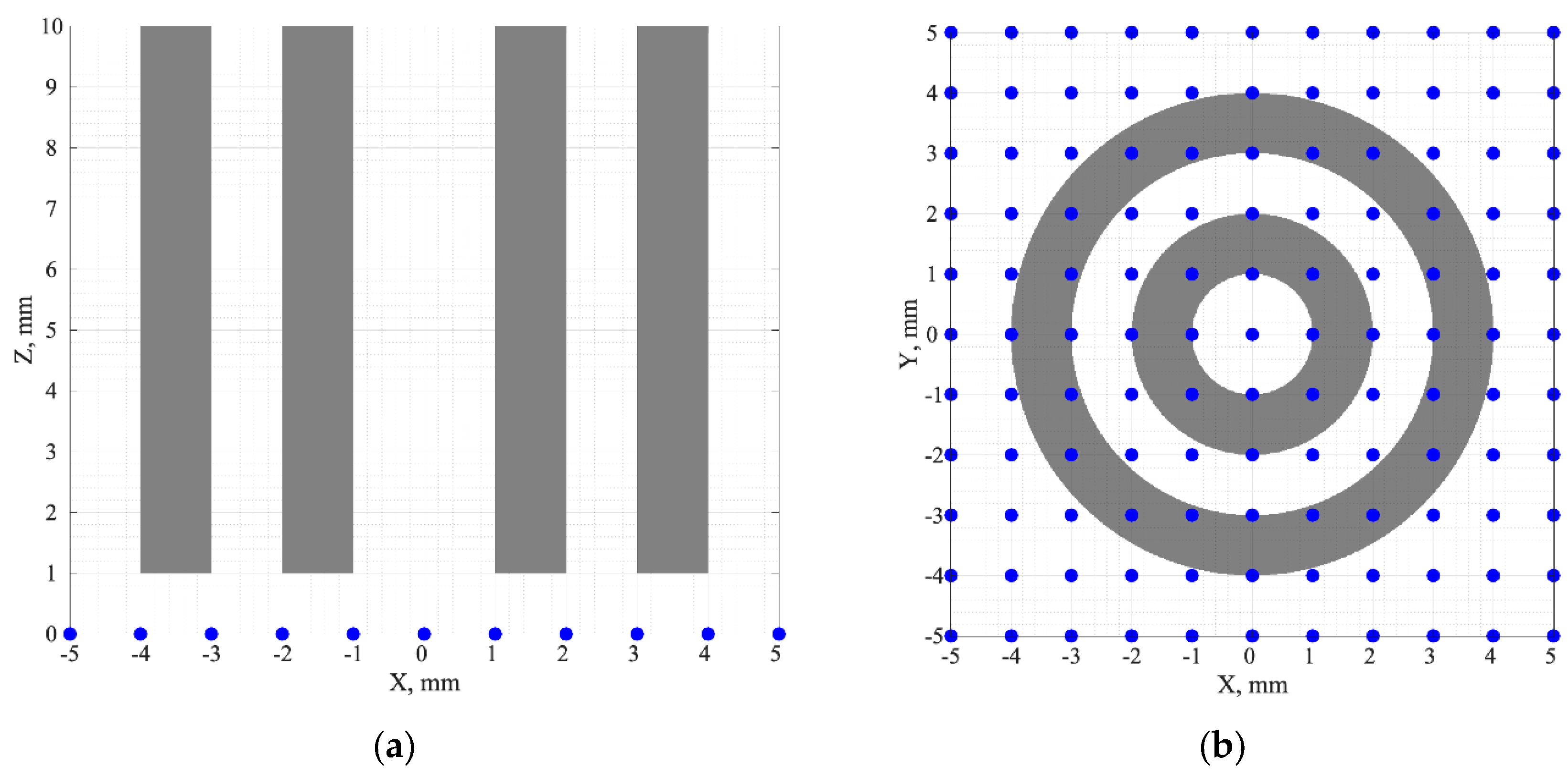
Figure 2.
Formation of SD links for the source at: (a) the point (0, 0, 0); (b) the point (1 mm, 1 mm, 0). In Figure 2(a), the unique SD links are shown in green, and the non-unique ones, in grey. In Figure 2(b), all the working SD links are green, the red dashed lines show the links that do not exist and are not hence considered.
Figure 2.
Formation of SD links for the source at: (a) the point (0, 0, 0); (b) the point (1 mm, 1 mm, 0). In Figure 2(a), the unique SD links are shown in green, and the non-unique ones, in grey. In Figure 2(b), all the working SD links are green, the red dashed lines show the links that do not exist and are not hence considered.
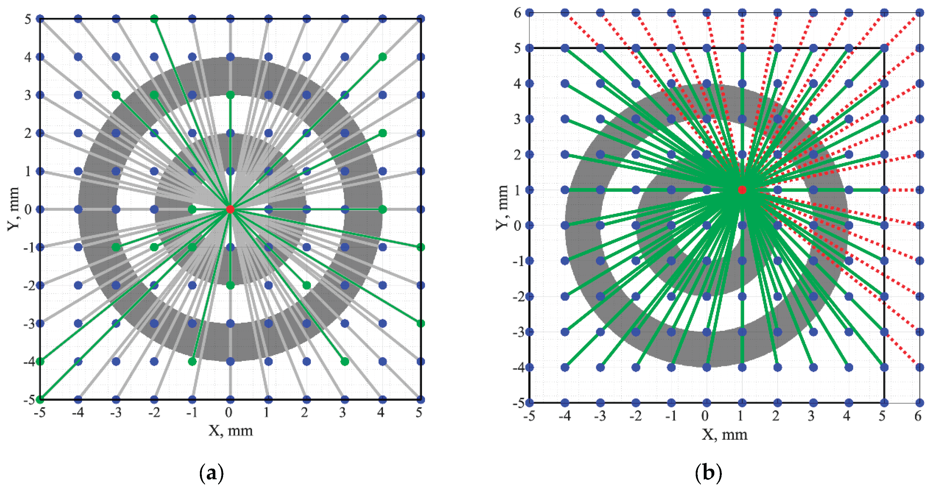
Figure 3.
The fluorescence signals calculated for the SD links of: (a) Figure 2(a), (b) Figure 2(b).
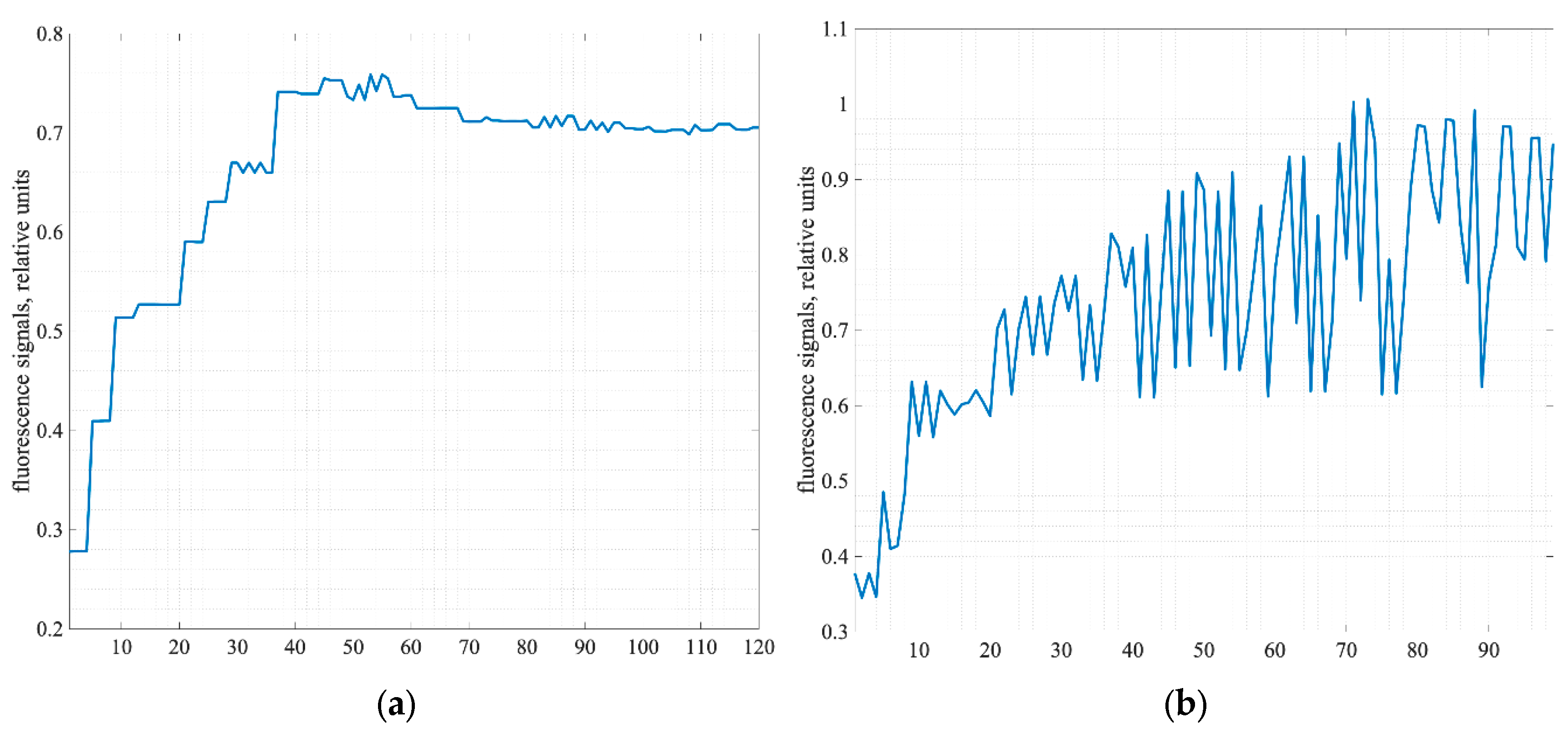
Figure 4.
The informative sections of 3D SSFs calculated for: (a) phantom without optical clearing, (b) phantom with the cleared surface layer (shown by the white line).
Figure 4.
The informative sections of 3D SSFs calculated for: (a) phantom without optical clearing, (b) phantom with the cleared surface layer (shown by the white line).
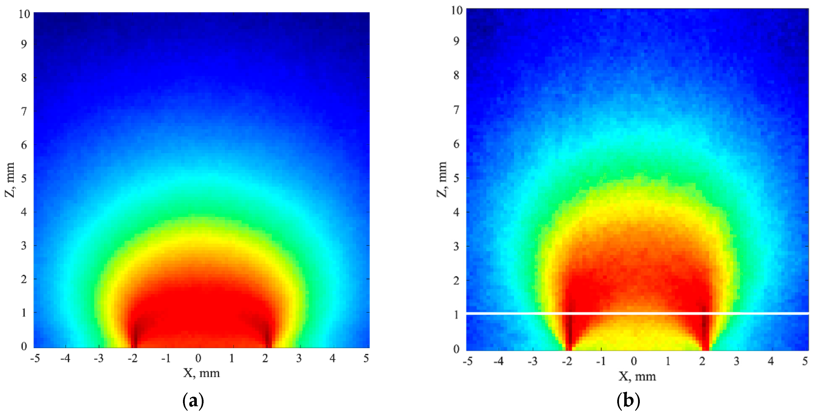
Figure 5.
The frontal sections of: (a) phantom with fluorophore, (b) 3D reconstruction for phantom without optical clearing, (c) 3D reconstruction for phantom with optical clearing.
Figure 5.
The frontal sections of: (a) phantom with fluorophore, (b) 3D reconstruction for phantom without optical clearing, (c) 3D reconstruction for phantom with optical clearing.
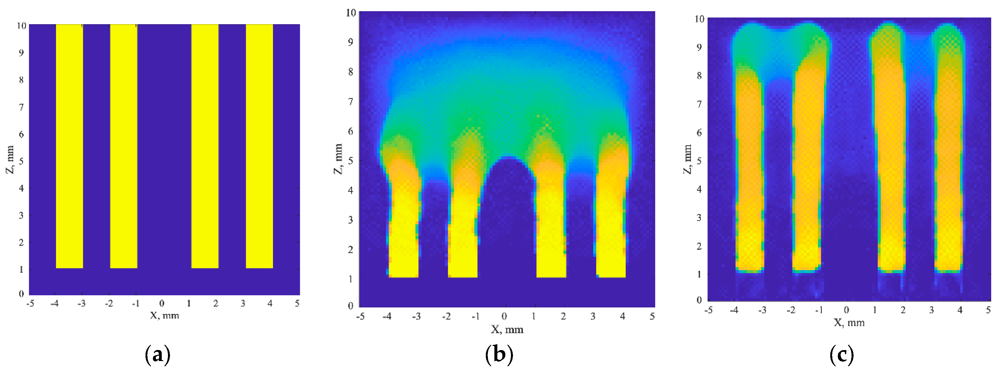
Figure 6.
Cross-sections of 3D reconstructions by the planes z = 3 mm (left); z = 5 mm(center); and z = 7 mm (right) for: (a) phantom without optical clearing, (b) phantom with optical clearing.
Figure 6.
Cross-sections of 3D reconstructions by the planes z = 3 mm (left); z = 5 mm(center); and z = 7 mm (right) for: (a) phantom without optical clearing, (b) phantom with optical clearing.
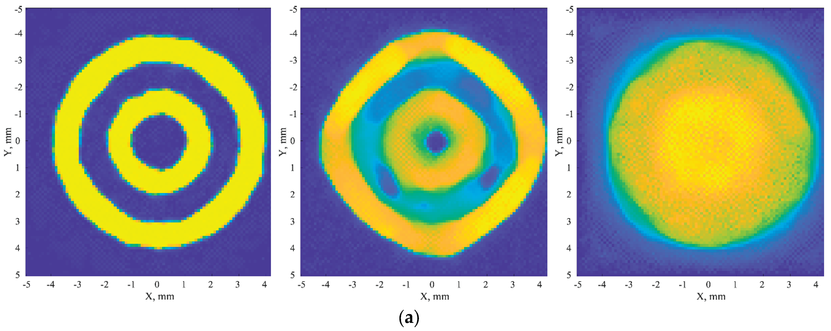
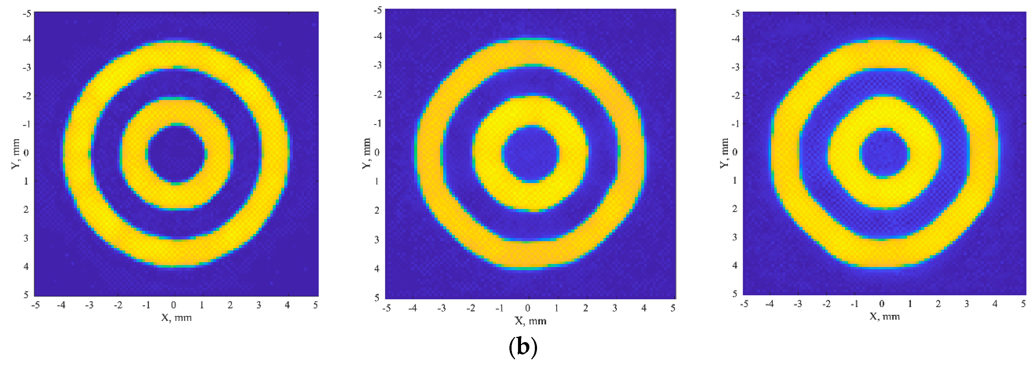
Figure 7.
The scheme of the modulation transfer coefficient evaluation: (a) one of cross-sections of 3D reconstruction with 8 radial directions, (b) the family of 8 profiles corresponding to 8 radial directions.
Figure 7.
The scheme of the modulation transfer coefficient evaluation: (a) one of cross-sections of 3D reconstruction with 8 radial directions, (b) the family of 8 profiles corresponding to 8 radial directions.
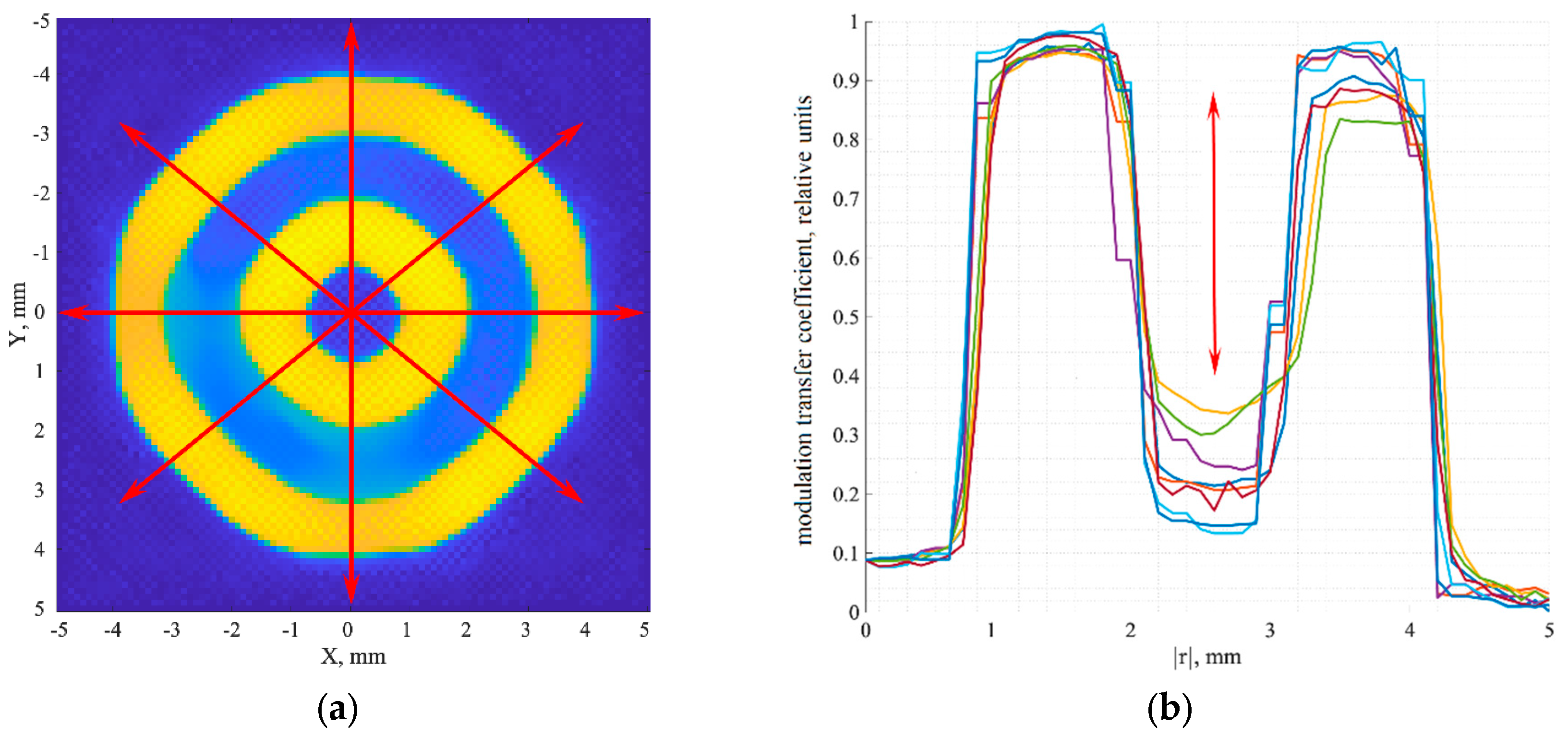
Figure 8.
The dependences of the modulation transfer coefficient on depth for the non-cleared (green) and cleared (blue) phantoms. The red line shows the 20% contrast corresponding to the Foucault-Rayleigh criterion.
Figure 8.
The dependences of the modulation transfer coefficient on depth for the non-cleared (green) and cleared (blue) phantoms. The red line shows the 20% contrast corresponding to the Foucault-Rayleigh criterion.
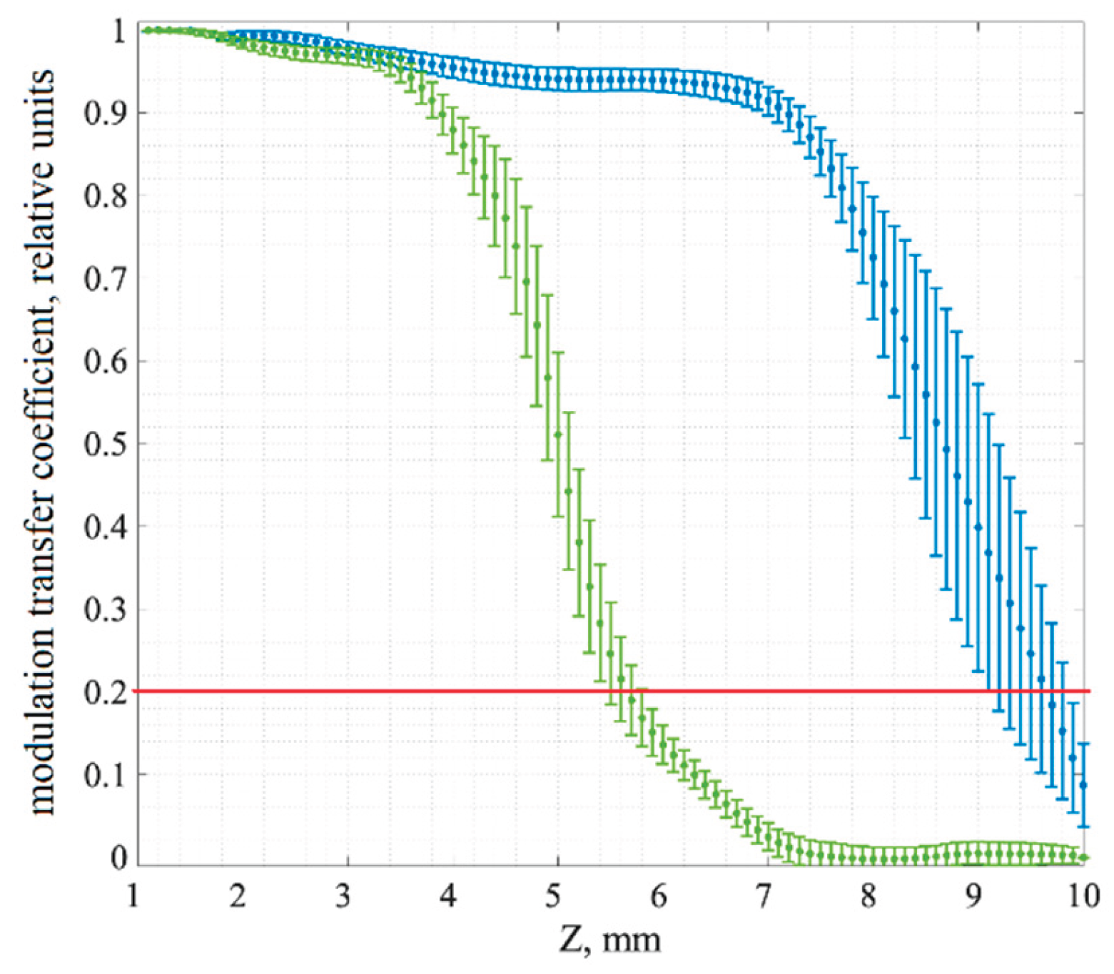

Table 1.
Optical parameters of the phantom before and after clearing of a thin surface layer.
| Parameter | Parameter value | |
| Before clearing | After clearing | |
| Thin surface layer (1 mm) | ||
| Absorption coefficient, μa, mm-1 |
0.01 | 0.01 |
| Scattering coefficient, μs, mm-1 |
10 | 5 |
| Anisotropy factor, g |
0.9 | 0.95 |
| Refractive index, n |
1.4 | 1.42 |
| Thick phantom layer (9 mm) | ||
| Absorption coefficient, μa, mm-1 |
0.01 | 0.01 |
| Scattering coefficient, μs, mm-1 |
10 | 10 |
| Anisotropy factor, g |
0.9 | 0.9 |
| Refractive index, n |
1.4 | 1.4 |
Table 2.
Fluorescence parameters.
| Parameter | Parameter value |
| Fluorophore absorption coefficient, μaf, mm-1 |
0.17 |
| Fluorophore scattering coefficient, μsf, mm-1 |
0 |
| Fluorescence quantum yield, γ |
0.48 |
| Fluorescence lifetime, τ, ps |
2200 |
Disclaimer/Publisher’s Note: The statements, opinions and data contained in all publications are solely those of the individual author(s) and contributor(s) and not of MDPI and/or the editor(s). MDPI and/or the editor(s) disclaim responsibility for any injury to people or property resulting from any ideas, methods, instructions or products referred to in the content. |
© 2026 by the authors. Licensee MDPI, Basel, Switzerland. This article is an open access article distributed under the terms and conditions of the Creative Commons Attribution (CC BY) license (http://creativecommons.org/licenses/by/4.0/).
Copyright: This open access article is published under a Creative Commons CC BY 4.0 license, which permit the free download, distribution, and reuse, provided that the author and preprint are cited in any reuse.