

Submitted:
02 November 2026
Posted:
04 November 2026
You are already at the latest version
Abstract
In complex underwater acoustic environments, biases in the effective sound speed and propagation-delay estimation errors may introduce skewness and heavy tails into measurement noise, thereby degrading maneuvering target tracking accuracy. Under these conditions, noise parameter estimates obtained through per-time-step variational updates are susceptible to measurement outliers, while coupling among parameters may hinder effective parameter updates. To exploit recent observations and improve parameter estimation stability, this paper proposes an adaptive interacting multiple model sliding-window variational Bayesian unscented filtering algorithm. Within the interacting multiple-model framework, variational inference and the unscented transform are combined to estimate the target state and noise-related variables at each time step. Sliding-window parameter fusion is applied to the location parameter and mixing variable, while sliding-window maximum a posteriori estimation is employed to update the shape parameter. Furthermore, an adaptive process noise covariance adjustment strategy based on changes in model probabilities is developed to balance rapid response to target maneuvers with robust tracking during steady motion. Simulation and lake-trial results demonstrate that the proposed algorithm outperforms the benchmark methods under skewed heavy-tailed measurement noise and target maneuvers. In the lake trial, the mean position and velocity tracking errors are reduced by 54.5% and 10.7%, respectively.
Keywords:
maneuvering target tracking
; variational Bayesian inference
; sliding-window parameter
; adaptive process noise
1. Introduction
Advances in unmanned underwater platforms and acoustic sensing technologies have increased the need for accurate underwater maneuvering target tracking. By recursively estimating target states from noisy acoustic measurements, tracking algorithms support underwater vehicle localization, navigation, and marine monitoring. Maintaining estimation accuracy in the presence of target maneuvers and complex measurement noise remains a key challenge.
Maneuvering target tracking requires accurate state estimation from noisy measurements while accommodating changes in target motion. Within the Bayesian estimation framework, various filtering methods have been developed, including the Kalman filter (KF) [1,2], extended Kalman filter (EKF) [3,4], unscented Kalman filter (UKF) [5,6,7], and particle filter (PF) [8]. The UKF uses the unscented transform to approximate the mean and covariance of random variables undergoing nonlinear transformations and has been applied to underwater maneuvering target tracking. The PF can address more general nonlinear, non-Gaussian estimation problems, although its estimation performance and computational cost depend on the number of particles and the resampling strategy[9]. These methods provide a foundation for target state estimation; however, reliance on a single fixed motion model may lead to model mismatch when the target switches between motion modes, thereby degrading tracking performance.
To address model mismatch caused by changes in target motion, the interacting multiple model (IMM) algorithm improves adaptability through model interaction, parallel filtering, and model-probability-weighted fusion. Li et al. [10] developed a Bayesian filtering framework incorporating delayed measurements to address random measurement delays and model switching in underwater target tracking, with adaptive adjustment of model transition probabilities. Yang et al. [11] combined adaptive and robust filtering within the IMM framework to address simultaneous process and measurement modeling errors. Guo et al. [12] introduced a maneuver-adaptive model set to improve adaptability to target maneuvers compared with a fixed model set. More recently, Zheng et al. [13] combined variational Bayesian estimation with a multiple-model approach for underwater extended target tracking with inaccurate noise covariances. Although these studies enhance model adaptability in different ways, the choice of process noise covariance still affects the trade-off between responsiveness to maneuvers and steady-state estimation error. Adapting the process noise covariance to changes in target motion therefore offers a means of improving maneuvering target tracking performance.
In addition to model mismatch caused by target maneuvers, non-Gaussian measurement noise also limits underwater tracking performance. To address estimation errors caused by measurement outliers, Stojanovic and Nedic [14] investigated robust nonlinear Kalman filtering under non-Gaussian noise. Whereas robust update schemes reduce the influence of measurement outliers, heavy-tailed distribution models explicitly characterize the probability of large errors. Roth et al. [15] modeled both process and measurement noise using Student’s t distributions and developed a robust filtering method for linear systems. Huang et al. [16] extended Student’s t filtering and smoothing to nonlinear systems, using the unscented transform to approximate the associated weighted integrals. Xue et al. [17] developed a robust filtering framework based on elliptically contoured distributions and employed a multiple-model mechanism to adaptively select the noise distribution, improving adaptability to different noise conditions. In underwater acoustic ranging, however, range estimates are affected by errors in both the effective sound speed and propagation-delay estimates. Sound speed variations, multipath propagation, and erroneous delay estimates may introduce systematic biases and large measurement errors[18]. When measurement errors exhibit both skewness and heavy tails, symmetric heavy-tailed distributions or symmetric noise mixture models may not adequately characterize their statistical properties, and the resulting noise model mismatch may further degrade tracking accuracy. Huang et al. [19] proposed a robust Kalman filtering framework based on Gaussian scale mixture distributions, employing variational Bayesian inference to estimate the state and noise-related variables under heavy-tailed and skewed noise. For skew-t measurement noise, Nurminen et al. [20] improved the treatment of dependencies among variables in the posterior approximation and incorporated expectation propagation to improve covariance estimation. To address nonstationary noise in underwater target tracking, Zhou et al. [21] modeled process noise and measurement noise using heavy-tailed and skewed distributions, respectively, and combined variational Bayesian estimation with distributed fusion for state estimation across multiple platforms. These studies provide a methodological foundation for state estimation under skewed heavy-tailed noise, while the update strategies for noise-related parameters remain important determinants of model adaptability and estimation performance.
Sliding-window estimation has recently been incorporated into adaptive robust filtering to make greater use of recent observations in noise parameter estimation. Wang et al. [22] modeled heavy-tailed measurement noise using a Pearson type VII distribution and jointly updated the state and noise-related parameters through state smoothing and variational iterations within the window. Based on a Bernoulli-Gaussian measurement model, Jiang et al. [23] developed centralized and distributed variational Bayesian moving horizon estimation methods to jointly estimate the state trajectory and unknown noise parameters within the window. For vessel tracking under heavy-tailed noise and random transmission delays, Liu et al. [24] combined a Student’s t noise model, measurement time alignment, and variational Bayesian moving horizon estimation. These studies improve the use of information from multiple time steps through state and parameter estimation within a moving window. For recursive tracking, further investigation is warranted into how recent local estimates can improve the stability of parameter updates without repeatedly solving for the joint posterior of the state trajectory and parameters within the window.
To address the above issues, this article proposes an Adaptive Interacting Multiple Model Sliding-Window Variational Bayesian Unscented Filter (AIMM-SWVBUF). The main contributions are summarized as follows:
- 1.
- A recursive estimation method combining per-time-step variational updates with sliding-window parameter fusion is developed under a generalized hyperbolic skewed Student’s t (GHSST) measurement noise model. The target state and noise-related variables are estimated using the unscented transform, while estimates of the location parameter and mixing variable are fused within the window to reduce the influence of fluctuations in local estimates on subsequent filtering updates.
- 2.
- A sliding-window maximum a posteriori (MAP) estimation method is developed to address the experimentally observed tendency of shape parameter estimates to remain near their initial values with limited updates. By combining observations from multiple time steps within the window with the parameter prior, the method updates the shape parameter separately to improve its estimation.
- 3.
- An adaptive process noise covariance adjustment strategy based on changes in model probabilities is designed. The strategy dynamically adjusts the process noise covariance in response to changes in target motion, balancing responsiveness during maneuvers with tracking accuracy during steady motion.
2. Materials and Methods
2.1. Problem Formulation
Establishment of a Nonlinear State-Space Model:
Where, k denotes the discrete time index, and is the state vector, and represent the target position and velocity components in a two-dimensional Cartesian coordinate system, respectively, and denotes the target turn rate. The measurement vector is denoted by . is the state transition matrix corresponding to the current motion model, and is the process noise weighting matrix. The function denotes the nonlinear measurement function. The vectors and represent the process noise and the measurement noise, respectively, and they are assumed to be mutually independent.
In complex underwater environments, the combined effects of acoustic propagation mechanisms and highly variable environmental conditions cause the measurement noise to exhibit both skewness and heavy-tailed characteristics. First, the skewness of the noise mainly originates from systematic biases and asymmetries in acoustic propagation paths. On the one hand, the sound speed profile, which is influenced by temperature, salinity, and depth, shows significant spatiotemporal inhomogeneity [25], leading to systematic errors in the estimation of the effective sound speed. As a result, range measurements statistically deviate from the zero-mean symmetric assumption. On the other hand, multipath propagation introduces asymmetries in both energy distribution and arrival times between the direct path and reflected paths [18], which further yields asymmetric components in the measurement errors. Second, the heavy-tailed nature of the noise is mainly attributed to complex environmental interference and outliers. During active sonar operation, reverberation severely interferes with time-delay estimation, inducing measurement outliers. Meanwhile, impulsive noise, ship-radiated noise, and biological noise that are ubiquitous in underwater environments [26] can easily introduce outliers into the measurement data, causing the noise distribution to exhibit heavy-tailed behavior. In summary, multiple physical factors jointly break the symmetry and stationarity of the noise distribution, giving rise to a dual non-Gaussian nature characterized by both nonzero-mean skewness and heavy tails. Under such conditions, the conventional zero-mean Gaussian assumption or purely symmetric heavy-tailed models become seriously mismatched to the actual noise statistics. Therefore, in this article, the process noise is modeled as Gaussian to represent random perturbations in the target motion, while the contaminated measurement noise is modeled by a Generalized Hyperbolic Skewed Student’s t (GHSST) distribution to accommodate the complex underwater acoustic observation environment. This distribution can be expressed in the form of a Gaussian-inverse-gamma mixture as follows [19].
Where denotes the process noise covariance matrix, is the location parameter of the measurement noise, accounting for an additive bias, is the measurement noise scale matrix, is the latent mixing variable, is the shape parameter governing the distribution’s skewness, is the degrees-of-freedom parameter, and denotes the inverse-gamma distribution.
The measurement equation can be expressed as:
Where denote the locations of the three observation points, respectively. The observation geometry is shown in Figure 1.
2.2. Overall Architecture
The AIMM-SWVBUF consists of three key components. First, the proposed Sliding-Window Variational Bayesian Unscented Filter (SWVBUF) is employed as the core estimation algorithm to perform joint inference of the state and noise parameters under skewed heavy-tailed measurement noise. Second, an IMM mechanism is introduced to achieve maneuvering target tracking through parallel model-conditioned filtering and probabilistic model updating. Finally, an adaptive process noise covariance adjustment is designed, which dynamically adjusts the noise parameters based on the changes in model probabilities, thereby achieving a balance between rapid maneuver response and high steady-state accuracy. Its schematic structure is shown in Figure 2.
2.3. Sliding-Window Variational Bayesian Unscented Filter
The following derivation focuses on the single-model formulation. The extension to the IMM-based multi-model framework will be detailed in Section 2.4. For notational simplicity, the model index is omitted in the subsequent derivations.
2.3.1. Single-Step Variational Inference
According to (1)-(3), the one-step predictive probability density function and the likelihood function can be expressed as follows:
Where denotes the system state at time k, represents the measurement set from time 1 to , is the one-step predicted state mean, and is the corresponding one-step predicted state covariance matrix.
To compensate for the systematic measurement errors caused by biases in the effective sound speed in underwater environments, is introduced as an unknown parameter to characterize the persistent nonzero-mean bias. Meanwhile, to further describe the heavy-tailed and skewed characteristics of the dual noise sources in complex underwater acoustic environments, is introduced, and the joint estimation of and is carried out within the variational inference framework. Specifically, is assumed to follow a Gaussian prior, while follows an inverse-gamma prior distribution. Combined with (6), the modified conditional likelihood function and parameter prior distributions are defined as follows:
Let the set of latent variables at time k be denoted by . Since direct analytical evaluation of the posterior distribution is intractable, a variational Bayesian approach is adopted to seek a tractable approximation to the true posterior. This problem is equivalent to minimizing the Kullback-Leibler divergence (KLD) between the two distributions [27].
To obtain a tractable analytical solution, based on the mean-field theory[28], the variational approximation is assumed to factorize into a product of independent components:
Since is a constant, minimizing the KLD is equivalent to maximizing the Evidence Lower Bound (ELBO)[28]:
The factors are iteratively updated using the Coordinate Ascent Variational Inference algorithm. For any element in , its optimal variational posterior update is given by:
Where denotes the expectation with respect to all variables in except , and is a normalization constant.
Next, taking the -th iteration as an example, the update procedures for the posterior estimate of the target state, the posterior estimate of the measurement-noise mean, and the posterior estimate of the mixing parameter are provided.
Let . As shown in Appendix B, its posterior distribution follows a Gaussian distribution. Therefore, the VB update can be written as:
Where and can be computed as follow:
Let . As shown in Appendix C, its posterior distribution follows a Gaussian distribution. Therefore, the VB update can be written as:
Where and can be computed as follows:
Let . As shown in Appendix D, its posterior distribution follows the generalized inverse gaussian (GIG) distribution. Therefore, the VB update can be written as:
Where can be computed as:
Since computing the moments of the GIG distribution requires evaluating modified Bessel functions of the second kind, its numerical implementation is relatively complicated and introduces additional computational burden. To ensure the real-time implementation of the algorithm, a MAP approach is adopted in this paper, where the complete posterior distribution is approximated by its mode, thereby yielding the update of :
To reduce computational complexity and avoid unnecessary repeated calculations, a convergence criterion is established for the variational Bayesian fixed-point iteration process. The iterative update is terminated when the relative change between the posterior state estimates obtained in two successive iterations satisfies the following condition:
Where denotes the convergence threshold, and represents the Euclidean norm.
This criterion uses the relative variation of the state estimate as the basis for convergence. When the update magnitude falls below the predefined threshold, the algorithm is considered to have reached a stable state, and the iteration is terminated. Furthermore, to ensure numerical stability under extreme conditions, a maximum number of iterations is specified, and the iteration process is forcibly stopped once this upper bound is reached.
2.3.2. Sliding-Window Parameter Fusion
In recursive Bayesian estimation, information from past observations can be propagated to the current time step through the prior distribution. Therefore, a recursive update at a single time step does not imply that only the current observation is used. In practical variational inference, however, parameter estimation performance depends on the approximate posterior structure, the prior propagation scheme, and the quality of the current measurement. Under skewed heavy-tailed measurement noise, measurement outliers may cause substantial fluctuations in local parameter estimates, thereby compromising the stability of target state estimation.
To mitigate these fluctuations, a sliding-window parameter fusion mechanism is introduced following the per-time-step variational update. For noise statistics that vary slowly over short time intervals, local estimates from recent time steps are fused to obtain parameter estimates at the current time step.
This subsection considers the fusion of estimates of the location parameter and the mixing variable . To distinguish these estimates from those obtained during the iterations, let and denote , respectively, the posterior mean of the location parameter and the MAP estimate of the mixing variable after termination of the variational iterations, but before sliding-window fusion. Define
Let L denote the prescribed window length. For , the sliding window comprises the L most recent time steps:
The effective window length is defined as the number of local estimates included in the fusion:
During initialization, the effective window length is used as the normalization factor in the averaging operation. Once the window is full, .
For the location parameter, slow variation within the window is assumed:
Under this assumption, local estimates of the location parameter at different time steps can be approximately regarded as estimates of a common offset. Fusing these estimates can mitigate fluctuations in per-time-step estimates. The mixing variable characterizes the random scale of the measurement at each time step and is allowed to vary across observations. Its estimates are also smoothed over the window as an additional algorithmic approximation. The resulting estimate is used in subsequent filtering computations and is not interpreted as a single underlying mixing variable shared across all time steps within the window.
To fuse the local estimates of the location parameter and the mixing variable within a unified formulation, the following objective function is constructed using a weighted least-squares criterion:
Where, is a positive definite diagonal weighting matrix.
Taking the gradient of (43) with respect to yields
Since the Hessian is positive definite, the objective function is strictly convex. Setting the gradient in (44) to zero gives the unique stationary point:
The positive definite diagonal structure of the weighting matrices ensures that each component of the fused estimate is a convex combination of the corresponding local estimates. Because , the fused mixing variable remains strictly positive. Therefore, (45) is feasible and constitutes the unique global minimizer of (43) over the specified domain.
For computational simplicity, a common weighting matrix is assigned to all time steps within the window:
Where, is a fixed positive definite diagonal matrix. Substituting (46) into (45) reduces the fusion rule to an arithmetic average:
The resulting parameter updates are
Equation (48) performs sliding-window averaging of the local posterior means of the location parameter and the local MAP estimates of the mixing variable. For , the updates reduce to the corresponding local estimates at the current time step.
2.3.3. Sliding-Window MAP Estimation
As shown in Figure 3, the estimates obtained by the joint variational inference method in [19] remain essentially around the initial value over the tracking sequence, exhibiting only slight fluctuations and showing no clear tendency to converge toward the true parameter value. This indicates that, under the joint variational inference framework, the posterior update of is subject to strong coupling constraints and suffers from insufficient identifiability, thereby limiting its correction capability. To address this issue, is no longer treated as a complete latent variable in the joint variational inference at the current time step; instead, a sliding-window MAP scheme is adopted for its separate estimation. By incorporating observations from multiple adjacent time steps within the window, the proposed method strengthens the statistical support for estimation and thereby improves its identifiability. The results show that the proposed method enables the estimate of to move away from the initial value and gradually approach the true value, indicating that the proposed estimation strategy effectively overcomes the stagnation problem in variational updating and achieves an effective update of . Furthermore, a more accurate estimate of helps improve the modeling accuracy of skewed heavy-tailed noise and ultimately enhances state tracking performance.
On this basis, a sliding-window MAP estimation model for is further established. Specifically, within a sliding window of length L, denoted by , is assumed to remain constant and to follow a Gaussian prior distribution:
Where and denote the prior mean and prior covariance, respectively.
Then, the sliding-window MAP estimate of is defined as:
Where denotes the set of latent variables other than , which have already been estimated by variational Bayesian inference.
According to (9), can be written as:
Where . (51) can be further expressed as:
Taking the derivative of (53) with respect to and setting it to zero yields:
Therefore, the closed-form solution is obtained as:
During initialization, single-time-step MAP estimation is used to update the shape parameter until the sliding window is full. The corresponding update is given by
2.4. IMM-Based Multi-Model Extension
2.4.1. Model Interaction
The model interaction step mixes the posterior state estimates of all models at time using the Markov transition probability matrix, thereby providing the initial conditions for each model filter at time k. Assume that the system consists of N models, and the transition probability from model i to model j is denoted by .
First, the mixing probability from model i to model j is computed as:
Where denotes the probability of model i at time , and denotes the predicted probability of model j at time k, which also serves as the normalization constant.
Based on the above mixing probabilities, the mixed initial state and the mixed initial covariance for model j at time k can be computed as:
Where . and denote the posterior state estimate and covariance estimate of model i at time , respectively. The mixed initial state and the mixed initial covariance are then used as inputs to the filter matched to model j at time k.
2.4.2. Model Filtering
For each motion model, the SWVBUF described in Section 2.3 is executed independently using the corresponding mixed initial state and covariance obtained from the model interaction step. Specifically, conditioned on the current motion model, the state and noise parameters are jointly estimated through the sliding-window variational Bayesian inference procedure.
It is worth emphasizing that the internal structure of the SWVBUF remains unchanged across different models; the only difference lies in the model-specific state transition matrix and process noise configuration.
2.4.3. Model Probability Update
After completing the variational iterations, the likelihood function of each model is updated using the corrected innovation residual .
The likelihood value and the model probability of model j are then computed as:
2.4.4. State Estimate Fusion
Finally, the global state estimate and the corresponding covariance matrix are obtained by a weighted sum of the filtering results of all models as follows:
2.5. Adaptive Process Noise Covariance Adjustment
In underwater maneuvering target tracking, the setting of the process noise covariance matrix involves a trade-off between response speed and tracking accuracy. When is chosen too large, excessive random perturbations are introduced during steady-state phases, degrading tracking accuracy. Conversely, when is too small, the filter fails to promptly adapt to rapid state variations during target maneuvers, resulting in delayed response. To resolve this dilemma, an adaptive regulation strategy based on changes in model probabilities is proposed to achieve a dynamic balance between the two.
2.5.1. Construction of the Modification Function
Within the IMM framework, the model probability can reflect in real time the degree of matching between the target motion mode and model j. When the target is in steady motion, the probabilities of all models remain relatively stable; when a maneuver occurs, the probability of the corresponding maneuvering model exhibits a pronounced increasing trend. Therefore, the changes in model probabilities can serve as a sensitive indicator for maneuver detection.
The increment of the maneuvering model probability at time k is defined as:
Based on this increment, an adaptive modification function for the process noise is constructed as :
Figure 4 illustrates an example of the variation of the modification function.
2.5.2. Process Noise Covariance Regulation
On this basis, the modification term of the process noise covariance matrix is defined as:
where is the adaptive scaling matrix, defined as:
Where denotes the tolerance threshold and c is the process noise covariance inflation factor.
When the variation of model probabilities is small, i.e., the value of the modification function lies within , the target is regarded as being in a steady-state phase. In this case, , and the nominal process noise covariance is retained to avoid introducing unnecessary disturbances and to ensure high estimation accuracy. When the model probabilities exhibit abrupt variations such that , the target is considered to be in a maneuvering phase. Then, the process noise covariance is enlarged by a factor c, so as to enhance the filter responsiveness to rapid state changes.
By integrating the derivations presented in Section 2.3, Section 2.4 and Section 2.5. the complete procedure of the AIMM-SWVBUF algorithm can be obtained. The corresponding implementation pseudocode is summarized in Algorithm 1.
| Algorithm 1 Pseudocode of the Proposed AIMM-SWVBUF for One Time Step |
|
Require: , , , , , , , , , N, , , L, c, , Ensure: , |
2.6. Computational Complexity Analysis
This subsection analyzes the per-time-step computational complexity of the proposed AIMM-SWVBUF algorithm. The main computational costs arise from filtering updates within each model, sliding-window parameter fusion, sliding-window MAP estimation of the shape parameter, and model interaction and estimate fusion within the IMM framework. Let n and m denote the state and measurement dimensions. Let N denote the number of models, L the sliding-window length, and the number of sigma points used in the unscented transform. The computational complexity of each main step is summarized in Table 1.
For the single-model SWVBUF, let denote the number of variational iterations performed at the current time step. The corresponding computational complexity is
Where is the number of iterations required to satisfy the convergence criterion. For the tracking problem considered in this study, . With , the above expression simplifies to
Within the IMM framework, filtering updates are performed separately for N models. Model interaction involves computing the mixed state mean and covariance for each model, with a total computational complexity of . Model probability updating and final state estimate fusion incur computational costs of and , respectively. Adaptive process noise adjustment primarily involves evaluating changes in model probabilities and scaling the process noise covariance; it therefore does not alter the asymptotic order of the dominant computations. Consequently, the per-time-step computational complexity of AIMM-SWVBUF is bounded by
Equation (71) shows that the computational cost of the proposed algorithm depends primarily on the state dimension, the number of models, the number of variational iterations, and the window length. Figure 5 presents the number of variational iterations performed by AIMM-SWVBUF at each time step in the considered experiment, with a mean of approximately 6.4. A comparison of the measured execution times is provided in Section 3.4.
3. Results and Discussion
To evaluate the tracking performance of the proposed algorithm in complex underwater acoustic environments, a three-stage validation scheme is designed.
First, a parameter sensitivity analysis is conducted. Specifically, the sliding-window length and the process noise amplification factor are systematically swept to investigate their impacts on tracking accuracy. This enables the identification of an optimal parameter configuration that balances accuracy and computational efficiency, thereby establishing a baseline for the subsequent experiments.
Second, an ablation study is performed using the selected parameter configuration. A baseline algorithm and variants obtained by removing individual modules are compared with the complete algorithm to assess the contributions of sliding-window parameter fusion, adaptive process noise covariance adjustment, and sliding-window MAP estimation of the shape parameter to tracking performance.
Finally, comprehensive comparative experiments are conducted. Building upon the optimal parameter configuration and the validated effectiveness of each module, the proposed algorithm is compared with the Adaptive Interacting Multiple Model Unscented Kalman Filter (AIMM-UKF)[12], the Interacting Multiple Model Unscented Kalman Filter (IMM-UKF)[6], the Robust Student’s t Unscented Kalman Filter (STUKF)[16], the Student’s t -Generalized Hyperbolic Skewed Student’s t Kalman Filter (ST-GHSST-KF)[19], and Robust Distributed Variational Bayesian Moving Horizon Estimation with a Bernoulli-Gaussian Measurement Noise Model (R-DVB-MHE-BG)[23]. It is worth noting that STUKF, ST-GHSST-KF and R-DVB-MHE-BG were originally developed as single-model algorithms. To ensure fairness and validity in maneuvering target tracking scenarios, they are extended to the IMM framework in this study, thereby enabling a comprehensive evaluation of the proposed algorithm’s overall advantages in handling skewed heavy-tailed measurement noise and target maneuvers.
3.1. Simulation Setup
This simulation considers a two-dimensional underwater target tracking scenario. The target motion is modeled using the state-space formulation introduced in Section 2.1, and tracking is performed using a Constant Velocity (CV) model and a Constant Turn Rate (CT) model. The corresponding state transition matrices and noise weighting matrices follow those in [6]. The total sampling duration is 800 s, with a sampling interval of . The target motion models over different time periods are listed in Table 2.
The process noise and measurement noise are specified as follows:
Where is the noise scale matrix, denotes the location parameter, denotes the shape parameter , is a diagonal matrix whose diagonal elements are independent and identically distributed, is an auxiliary random vector, and the degrees of freedom are set to .
In this simulation, the parameters of all compared methods are configured according to the settings reported in the corresponding references. For the proposed algorithm, the prior parameters are set as follows: , , , , and . The initial target state is , the state covariance matrix is , The transition probability matrix is , the initial model probability is , The number of iteration is set as . All algorithms were implemented in MATLAB, and all simulation were performed on a computer equipped with an Intel Core i9-13900HX CPU @ 2.2 GHz and 64 GB of RAM.
Figure 6 shows the ground-truth trajectory of the maneuvering target and the locations of the three buoys. Figure 7 presents the range measurements obtained from the three buoys, and Figure 8 illustrates the probability density distributions of the measurement noise for the three buoys.
To evaluate the filtering performance, the root mean square error (RMSE) and the average RMSE (ARMSE) are employed as performance metrics. All results are obtained from 1000 independent Monte Carlo runs.
3.2. Parameter Sensitivity Analysis
3.2.1. Sliding-Window Length
Figure 9 illustrates the effect of the sliding-window length L on the position and velocity ARMSE. As the window length increases, the position ARMSE initially decreases markedly, while the velocity ARMSE decreases more gradually. The position ARMSE is lowest around , with relatively low values over , whereas the velocity ARMSE reaches its minimum at . Beyond , both metrics show an overall upward trend, although the velocity ARMSE exhibits minor local fluctuations. These results indicate that an appropriate window length helps reduce tracking errors by fusing local estimates from several recent time steps, thereby mitigating the influence of fluctuations in individual estimates on subsequent filtering updates. However, an excessively long window may incorporate historical information that no longer adequately represents the current state or noise characteristics, reducing the responsiveness of the estimator and increasing estimation errors. Therefore, considering both position and velocity estimation accuracy, is selected as the optimal window length among the configurations examined and is used in the subsequent experiments.
3.2.2. Process Noise Amplification Factor
Table 3 presents the impact of the process noise amplification factor c on the tracking performance of the algorithm. The results indicate that, as c increases within the range [1, 100], the ARMSE of both position and velocity decreases and reaches its minimum at . This phenomenon confirms the rationality of the proposed adaptive process noise covariance adjustment: when a target maneuver is detected, moderately increasing the process noise covariance can effectively increase the filter gain, thereby compensating for the lag induced by model mismatch and improving the responsiveness to maneuvering dynamics. However, when c is further increased to the range [100, 200] the ARMSE gradually rises, suggesting that an excessively large amplification factor makes the algorithm overly sensitive to measurement noise in steady-state phases, leading to unnecessary errors. In summary, to balance maneuver responsiveness and steady-state tracking accuracy, is selected as the optimal setting in the subsequent experiments.
3.3. Algorithm Ablation Experiments
To assess the contribution of each proposed module to tracking performance, an ablation study is conducted using five algorithm configurations. The complete AIMM-SWVBUF algorithm is denoted as Full, while IMM-VBUF, which incorporates none of the three proposed enhancements, is denoted as Baseline. Three variants—w/o Fusion, w/o MAP, and w/o Adapt—are obtained by individually removing sliding-window parameter fusion, sliding-window MAP estimation of the shape parameter, and adaptive process noise covariance adjustment from the complete algorithm, respectively. Table 4 summarizes the modules included in each configuration. Sliding-window parameter fusion, sliding-window MAP estimation of the shape parameter, and adaptive process noise covariance adjustment are described in Section 2.3.2, Section 2.3.3, and Section 2.5, respectively.
All algorithms are evaluated under the same simulation conditions and parameter settings. Figure 10 and Figure 11 present the position and velocity tracking RMSE curves, respectively, for the algorithms in the ablation study, while Table 5 reports the corresponding ARMSE values.
Compared with w/o Fusion, Full reduces the position and velocity ARMSE by approximately 26.3% and 4.8%, respectively. Sliding-window parameter fusion integrates local estimates from recent time steps, reducing the direct influence of fluctuations in individual estimates on subsequent filtering updates. These results indicate that the module contributes to lower tracking errors, with a more pronounced improvement in position estimation accuracy.
Compared with w/o MAP, Full reduces the position ARMSE by approximately 11.7%, while the velocity ARMSE remains essentially unchanged. Sliding-window MAP estimation of the shape parameter combines observations from multiple time steps within the window with the parameter prior to refine the prescribed shape parameter, allowing the noise model to adapt to the observations. These results suggest that the module primarily improves position tracking accuracy.
Compared with w/o Adapt, Full reduces the position and velocity ARMSE by approximately 9.6% and 7.2%, respectively, and also reduces the dominant error peaks following the onset of both turns. Adaptive process noise covariance adjustment responds to changes in model probabilities, improving the filter’s responsiveness to state changes during maneuvers and thereby mitigating tracking errors caused by motion model mismatch.
Overall, Full reduces the position and velocity ARMSE by approximately 32.3% and 19.6%, respectively, relative to Baseline. These results indicate that the combined use of the three enhancements reduces the average tracking error in the scenario considered.
3.4. Comprehensive Comparative Experiments
Figure 12 and Figure 13 show the RMSE curves of different algorithms for position and velocity, respectively, while Table 6 reports the corresponding average RMSE values.
Both IMM-UKF and AIMM-UKF are formulated under the Gaussian noise assumption, which does not fully capture the skewed heavy-tailed measurement noise considered in this study. AIMM-UKF employs a maneuver-adaptive model set to improve adaptability to changes in target motion. As shown in Table 6 AIMM-UKF achieves slightly lower position and velocity ARMSE values than IMM-UKF. However, both methods yield higher errors than the proposed algorithm under the considered noise conditions, indicating that improved motion-model adaptability alone may be insufficient to achieve robust tracking in the presence of skewed heavy-tailed measurement noise.
Although STUKF, ST-GHSST-KF and R-DVB-MHE-BG are designed for non-Gaussian noise and can suppress outliers to some extent, their performance is still limited by inherent bottlenecks. STUKF employs a prespecified degrees-of-freedom parameter, which limits its adaptability to changes in noise characteristics. Although ST-GHSST-KF models noise using Gaussian scale mixture distributions, its shape parameter estimates remain close to their initial values under the configuration considered, exhibiting only minor adjustments. This behavior may restrict the noise model’s ability to adapt to the observed measurements. R-DVB-MHE-BG combines a Bernoulli-Gaussian measurement model with moving horizon estimation to handle measurement outliers; however, its position and velocity ARMSE values remain higher than those of ST-GHSST-KF and the proposed algorithm.
In contrast, AIMM-SWVBUF achieves the best overall performance. Benefiting from the sliding-window mechanism that provides smoothed estimation of noise parameters and the adaptive process noise covariance adjustment that enables rapid response to maneuvers, the proposed method attains a superior balance between suppressing heavy-tailed noise and capturing strong maneuvers. As shown in Table 6, relative to the best-performing benchmark for each metric, the proposed algorithm reduces the position and velocity ARMSE by approximately 24.8% and 20.2%, respectively. These results demonstrate the high accuracy and strong robustness of AIMM-SWVBUF for maneuvering target tracking in complex underwater acoustic environments.
Table 7 compares the average execution times of three methods involving variational Bayesian iterations. To facilitate a fair comparison, convergence-based stopping criteria are also applied to the variational iterations of ST-GHSST-KF and R-DVB-MHE-BG. Under the same experimental conditions, AIMM-SWVBUF has a lower average execution time than the other two methods.
3.5. Validation Using Lake Trial Data
To validate the tracking performance of the proposed algorithm in a real underwater acoustic environment, an underwater target tracking experiment was conducted in June 2025 at an artificial lake. In the experiment, an acoustic transceiver was mounted beneath a small boat to serve as the underwater moving target, and a high-precision GPS positioning system was installed on the boat to provide the ground-truth target trajectory. Within an area of approximately , three positioning buoys (labeled S1-S3) were deployed. Each buoy was equipped with an acoustic transceiver and a GPS receiver, forming a distributed observation network. The GPS positioning information was updated at 1 Hz. The co-located transmit-receive transducers on the buoys transmitted probing signals to the target boat and received echoes every 2s, with a sampling interval of . All collected data were transmitted in real time to the mothership platform for logging and processing. The total sampling duration was 200s.
The experiment established a two-dimensional Cartesian coordinate system with the mothership as the origin. After coordinate transformation, the coordinates of the three positioning buoys are S1(-442.7085m, -192.0706m), S2(-783.0345, -579.1814m), S3(-38m, -318.8523m). For filter initialization, the process noise covariance is set to and the measurement noise scale matrix is . The GPS-measured initial position of the boat is (-230m, -253.08m). Accordingly, the initial state is set to and the initial state covariance matrix is . The remaining parameters are kept consistent with those used in the numerical simulations.
Figure 14 shows the ground-truth target trajectory and the buoy deployment layout, while Figure 15 presents the range measurements from the three buoys. By subtracting the GPS-derived geometric ranges from the acoustic range measurements at each time instant, the true measurement errors are obtained. Kernel density estimation (KDE) is then applied to the error sequence, producing the probability density curves shown in Figure 16. It can be observed that the measurement noise in the real underwater acoustic channel exhibits pronounced heavy-tailed and skewed characteristics, providing strong experimental evidence for adopting the GHSST distribution for noise modeling in this article.
Figure 17 and Figure 18 show the position and velocity estimation errors of different algorithms in the lake-trial experiment, respectively. The position average error values of the IMM-UKF, STUKF, ST-GHSST-KF, R-DVB-MHE-BG and AIMM-SWVBUF algorithms are 9.696 m, 9.398 m, 7.630 m, 10.681 m and 3.468 m, respectively, while the corresponding velocity average error values are 0.373 m/s, 0.412 m/s, 0.367 m/s, 0.308 m/s and 0.275 m/s. It can be seen that the proposed algorithm achieves the best performance in both metrics. Compared with the other algorithms, it reduces the average position error by more than 54.5% and the average velocity error by more than 10.7%. These results indicate that, in real underwater acoustic environments, the proposed algorithm can more effectively suppress the adverse effects of non-Gaussian skewed heavy-tailed noise and target maneuvering, thereby achieving higher tracking accuracy and robustness.
4. Conclusions
This paper proposes an adaptive interacting multiple-model sliding-window variational Bayesian unscented filtering algorithm to address fluctuations in local parameter estimates and insufficient updates of certain parameters under skewed heavy-tailed measurement noise, as well as motion model mismatch caused by target maneuvers. The method models measurement noise using a generalized hyperbolic skewed Student’s t distribution. Building on per-time-step updates, it applies sliding-window fusion to estimates of the location parameter and temporal smoothing to local MAP estimates of the mixing variable. It also updates the shape parameter through sliding-window MAP estimation and adaptively adjusts the process noise covariance based on changes in model probabilities. Simulation results demonstrate reductions in position and velocity tracking errors in the scenarios considered, while lake-trial results further validate the algorithm’s effectiveness and robustness in a complex underwater acoustic environment. Future work will investigate adaptive window-length selection, allowing the window length to vary with noise statistics and target motion to further improve parameter estimation stability and tracking performance.
Author Contributions
Conceptualization, T.J., X.M. and Y.L.; methodology, T.J.; validation, X.P.; resources, X.M.; data curation, P.L.; writing—original draft preparation, T.J.; writing—review and editing, T.J., X.P. and P.L.; supervision, Y.L.; funding acquisition, X.M. All authors have read and agreed to the published version of the manuscript.
Funding
This research was funded by the Application Innovation Project, grant number E590151201.
Institutional Review Board Statement
Not applicable.
Informed Consent Statement
Not applicable.
Data Availability Statement
The raw data supporting the conclusions of this article will be made available by the authors on request.
Acknowledgments
During the preparation of this manuscript, the authors used ChatGPT (OpenAI) to assist with translation, language refinement and grammatical corrections. All AI-assisted content was critically reviewed, edited, and verified by the authors, who take full responsibility for the accuracy, originality, and integrity of the final manuscript.
Conflicts of Interest
The authors declare no conflicts of interest.
Abbreviations
The following abbreviations are used in this manuscript:
| AIMM-SWVBUF | Adaptive interacting multiple model sliding-window variational Bayesian unscented filter |
| AIMM-UKF | Adaptive interacting multiple model unscented Kalman filter |
| ARMSE | Average root mean square error |
| CT | Constant turn rate |
| CV | Constant velocity |
| EKF | Extended Kalman filter |
| ELBO | Evidence lower bound |
| GHSST | Generalized hyperbolic skewed Student’s t |
| GIG | Generalized inverse Gaussian |
| GPS | Global Positioning System |
| IG | Inverse-gamma |
| IMM | Interacting multiple model |
| IMM-UKF | Interacting multiple model unscented Kalman filter |
| IMM-VBUF | Interacting multiple model variational Bayesian unscented filter |
| KDE | Kernel density estimation |
| KF | Kalman filter |
| KLD | Kullback–Leibler divergence |
| MAP | Maximum a posteriori |
| Probability density function | |
| PF | Particle filter |
| R-DVB-MHE-BG | Robust distributed variational Bayesian moving horizon estimation with a Bernoulli–Gaussian measurement noise model |
| RMSE | Root mean square error |
| ST-GHSST-KF | Student’s t–generalized hyperbolic skewed Student’s t Kalman filter |
| STUKF | Robust Student’s t unscented Kalman filter |
| SW | Sliding window |
| SWVBUF | Sliding-window variational Bayesian unscented filter |
| UKF | Unscented Kalman filter |
| UT | Unscented transform |
| VB | Variational Bayesian |
| w/o | Without |
Appendix A
To derive the update equations for each parameter, the joint probability density function of the system is constructed according to (5), (9) and (10).
Taking the logarithm of the joint probability and expanding it, while ignoring constant terms that are irrelevant to the parameters to be estimated, yields:
Where m is the dimension of the measurement vector, and denotes the bias-compensated measurement.
Appendix B
According to (16), take the expectation of the joint log-probability density with respect to all variables except . Substituting (A2) and collecting the terms related to , we obtain:
Where .
This expression is obtained using the expectation substitution approach, which approximates the intractable joint posterior by a tractable form with respect to .
Define the modified one-step predictive probability density function and the modified likelihood function as:
Where the corrected equivalent location parameter and the equivalent measurement-noise covariance are computed as:
Appendix C
According to (16), take the expectation of the joint log-probability density with respect to all variables except . Substituting (A2) and collecting the terms related to , we obtain:
Where can be computed as:
Define the modified one-step predictive density and the effective Gaussian likelihood as:
The variational posterior is proportional to the product of the Gaussian prior and the effective Gaussian likelihood. Therefore, it is also Gaussian.
Where and can be obtained using the standard Kalman filter update equations:
Appendix D
According to (16), take the expectation of the joint log-probability density with respect to all variables except . Substituting (A2) and collecting the terms related to , we obtain:
Where can be computed as:
According to the variational update equation, contains three types of terms simultaneously, namely , , and . Its functional form is therefore consistent with the logarithmic density of the GIG distribution. Hence, the posterior distribution of can be written in the following form:
However, in the subsequent state estimation and parameter update procedures, it is necessary to repeatedly compute the relevant statistics of . Since the first-order moment of the GIG distribution involves the modified Bessel function of the second kind, they usually do not admit simple closed-form evaluation, and numerical approximation or lookup operations are required at each time step and for each model. This introduces considerable additional computational burden, thereby affecting the real-time performance of the algorithm. To address this issue, a MAP approach is adopted in this paper, where is approximated by a Dirac delta distribution centered at its optimal solution :
This treatment replaces propagation of the full posterior distribution of the auxiliary variable with a point estimate. Although this approximation neglects higher-order uncertainty information associated with , it avoids repeated evaluation of GIG distribution moments and the associated special functions, thereby reducing computational complexity and balancing estimation accuracy with real-time computational requirements.
Let and . Then, (A25) can be rewritten as:
Taking the derivative of (A33) with respect to and setting it to zero yields:
Since , the unique positive root of this equation is taken as the updated value:
References
- Jondhale, S.R.; Deshpande, R.S. Kalman Filtering Framework-Based Real Time Target Tracking in Wireless Sensor Networks Using Generalized Regression Neural Networks. IEEE Sens. J. 2019, 19, 224–233. [Google Scholar] [CrossRef]
- Auger, F.; Hilairet, M.; Guerrero, J.M.; Monmasson, E.; Orlowska-Kowalska, T.; Katsura, S. Industrial Applications of the Kalman Filter: A Review. IEEE Trans. Ind. Electron. 2013, 60, 5458–5471. [Google Scholar] [CrossRef]
- Wang, S.; Zheng, H.; Zhang, T.; Li, J.; Xu, W. Frequency and Time of Arrival Based Moving Target State Estimation with Underwater Distributed Sensor Network. Ocean Eng. 2025, 334, 121563. [Google Scholar] [CrossRef]
- Stano, P.; Lendek, Z.; Braaksma, J.; Babuška, R.; de Keizer, C.; den Dekker, A.J. Parametric Bayesian Filters for Nonlinear Stochastic Dynamical Systems: A Survey. IEEE Trans. Cybern. 2013, 43, 1607–1624. [Google Scholar] [CrossRef] [PubMed]
- Kulikov, G.Yu.; Kulikova, M.V. Hyperbolic-SVD-Based Square-Root Unscented Kalman Filters in Continuous-Discrete Target Tracking Scenarios. IEEE Trans. Autom. Control 2022, 67, 366–373. [Google Scholar] [CrossRef]
- Wu, X.; Liu, Y.; Ma, X. An Underwater Maneuvering Target Tracking Algorithm Based on UKF with Adaptive Sampling Range. In Proceedings of the 2023 42nd Chinese Control Conference (CCC), Tianjin, China, 24–26 July 2023; pp. 3133–3138. [Google Scholar]
- Dong, Y.; Li, W.; Li, D.; Liu, C.; Xue, W. Intelligent Tracking Method for Aerial Maneuvering Target Based on Unscented Kalman Filter. Remote Sens. 2024, 16, 3301. [Google Scholar] [CrossRef]
- Fang, H.; Tian, N.; Wang, Y.; Zhou, M.; Haile, M.A. Nonlinear Bayesian Estimation: From Kalman Filtering to a Broader Horizon. IEEE/CAA J. Autom. Sin. 2018, 5, 401–417. [Google Scholar] [CrossRef]
- Kuptametee, C.; Aunsri, N. A Review of Resampling Techniques in Particle Filtering Framework. Measurement 2022, 193, 110836. [Google Scholar] [CrossRef]
- Li, X.; Lu, B.; Li, Y.; Lu, X.; Jin, H. Adaptive Interacting Multiple Model for Underwater Maneuvering Target Tracking with One-Step Randomly Delayed Measurements. Ocean Eng. 2023, 280, 114933. [Google Scholar] [CrossRef]
- Yang, B.; Wang, H.; Shi, Z. Interacting Multiple Model Adaptive Robust Kalman Filter for Process and Measurement Modeling Errors Simultaneously. Signal Process. 2025, 227, 109743. [Google Scholar] [CrossRef]
- Guo, J.-P.; Xu, J.; Yan, L.; Xia, X.-G.; Xiao, X.; Long, T.; Bian, M.-M. An Improved IMM Algorithm Based on Maneuvering-Adaptive Model Set. In Proceedings of the 2016 CIE International Conference on Radar (RADAR), Guangzhou, China, 10–13 October 2016; pp. 1–5. [Google Scholar]
- Zheng, X.; Zhang, Y.; Li, H. Underwater Maneuvering Extended Object Tracking with Inaccurate Noise Covariances. Ocean Eng. 2026, 359, 125986. [Google Scholar] [CrossRef]
- Stojanović, V.; Nedić, N. Robust Kalman Filtering for Nonlinear Multivariable Stochastic Systems in the Presence of Non-Gaussian Noise. Int. J. Robust. Nonlinear Control 2016, 26, 445–460. [Google Scholar] [CrossRef]
- Roth, M.; Özkan, E.; Gustafsson, F. A Student’s t Filter for Heavy Tailed Process and Measurement Noise. In Proceedings of the 2013 IEEE International Conference on Acoustics, Speech and Signal Processing (ICASSP), Vancouver, BC, Canada, 26–31 May 2013; pp. 5770–5774. [Google Scholar]
- Huang, Y.; Zhang, Y.; Li, N.; Chambers, J. Robust Student’s t Based Nonlinear Filter and Smoother. IEEE Trans. Aerosp. Electron. Syst. 2016, 52, 2586–2596. [Google Scholar] [CrossRef]
- Xue, C.; Huang, Y.; Zhu, F.; Zhang, Y.; Chambers, J.A. An Outlier-Robust Kalman Filter with Adaptive Selection of Elliptically Contoured Distributions. IEEE Trans. Signal Process. 2022, 70, 994–1009. [Google Scholar] [CrossRef]
- Jensen, F.B.; Kuperman, W.A.; Porter, M.B.; Schmidt, H. Computational Ocean Acoustics, 2nd ed.; Springer: New York, NY, USA, 2011. [Google Scholar]
- Huang, Y.; Zhang, Y.; Shi, P.; Wu, Z.; Qian, J.; Chambers, J.A. Robust Kalman Filters Based on Gaussian Scale Mixture Distributions with Application to Target Tracking. IEEE Trans. Syst. Man. Cybern. Syst. 2019, 49, 2082–2096. [Google Scholar] [CrossRef]
- Nurminen, H.; Ardeshiri, T.; Piché, R.; Gustafsson, F. Skew-t Filter and Smoother with Improved Covariance Matrix Approximation. IEEE Trans. Signal Process. 2018, 66, 5618–5633. [Google Scholar] [CrossRef]
- Zhou, L.; Zhang, G.; Huo, Y.; Wang, S.; Jin, Y. Distributed Target Tracking Based on Variational Bayesian Method under Non-Stationary Noises. Automatica 2026, 191, 113124. [Google Scholar] [CrossRef]
- Wang, K.; Wu, P.; Li, X.; He, S.; Li, J. An Adaptive Outlier-Robust Kalman Filter Based on Sliding Window and Pearson Type VII Distribution Modeling. Signal Process. 2024, 216, 109306. [Google Scholar] [CrossRef]
- Jiang, Z.; Battistelli, G.; Chisci, L.; Forti, N.; Zhou, W. Outlier-Robust Centralized and Distributed Variational Bayesian Moving Horizon Estimation. IEEE Trans. Signal Process. 2025, 73, 2527–2541. [Google Scholar] [CrossRef]
- Liu, B.; Wu, P.; He, S. A Variational Bayesian Moving Horizon Estimation Algorithm for Vessel Tracking under Heavy-Tailed Noise and Random Latency. Ocean Eng. 2026, 364, 126773. [Google Scholar] [CrossRef]
- Kinugasa, N.; Tadokoro, K.; Kato, T.; Terada, Y. Estimation of Temporal and Spatial Variation of Sound Speed in Ocean from GNSS-A Measurements for Observation Using Moored Buoy. Prog. Earth Planet. Sci. 2020, 7, 21. [Google Scholar] [CrossRef]
- Siderius, M.; Gebbie, J. Environmental Information Content of Ocean Ambient Noise. J. Acoust. Soc. Am. 2019, 146, 1824–1833. [Google Scholar] [CrossRef] [PubMed]
- Dong, X.; Battistelli, G.; Chisci, L.; Cai, Y. An Adaptive Consensus Filter for Distributed State Estimation with Unknown Noise Statistics. IEEE Signal Process. Lett. 2021, 28, 1595–1599. [Google Scholar] [CrossRef]
- Tzikas, D.G.; Likas, A.C.; Galatsanos, N.P. The Variational Approximation for Bayesian Inference. IEEE Signal Process. Mag. 2008, 25, 131–146. [Google Scholar] [CrossRef]
Figure 1.
Schematic of the three-station range-only observation scenario.
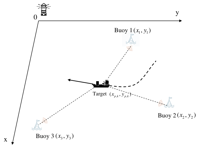
Figure 2.
Framework of the proposed algorithm.
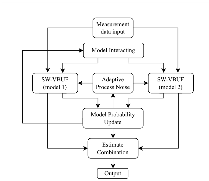
Figure 3.
Evolution of the shape parameter estimate.
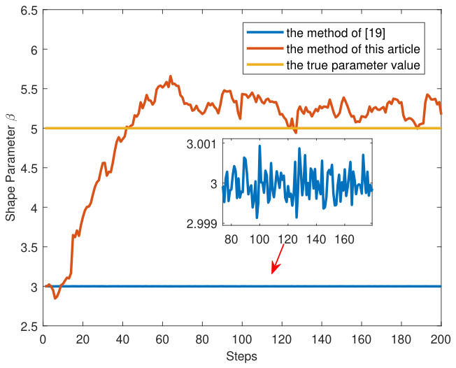
Figure 4.
Variation curve of the modification function.
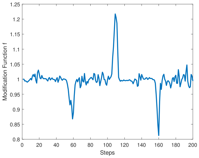
Figure 5.
Number of variational iterations at each time step.
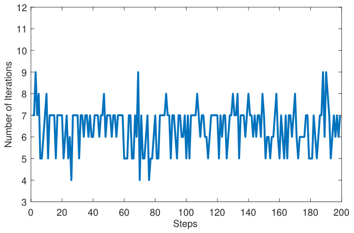
Figure 6.
Target trajectory and buoy layout in the simulation scenario.
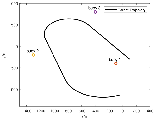
Figure 7.
Range measurements from the three buoys in the simulation scenario.
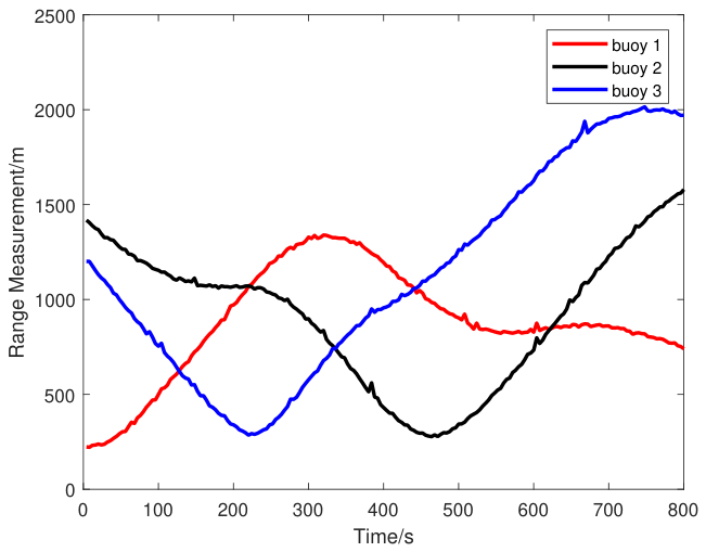
Figure 8.
Probability density functions of the measurement noise in the simulation scenario.
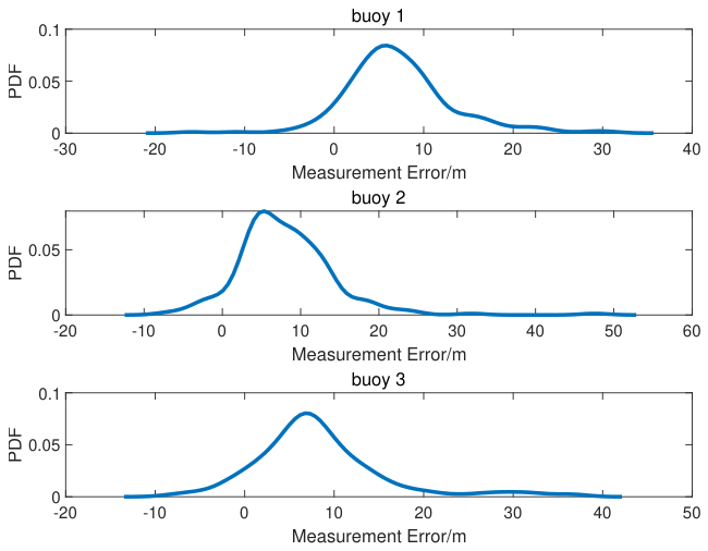
Figure 9.
Effect of the sliding-window length on the position and velocity ARMSE.
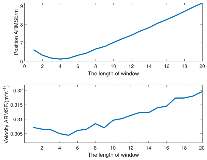
Figure 10.
Position RMSE of different algorithms in the ablation study.
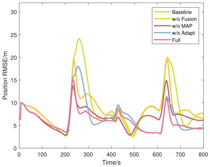
Figure 11.
Velocity RMSE of different algorithms in the ablation study.
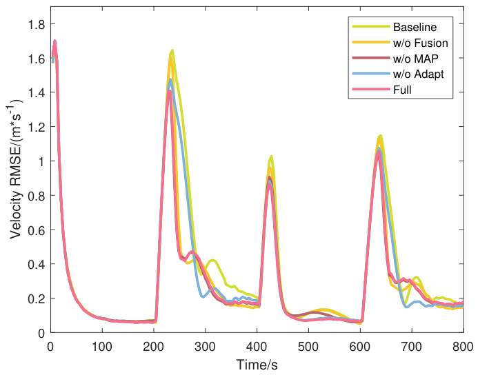
Figure 12.
Position RMSE of different algorithms in the simulation study.
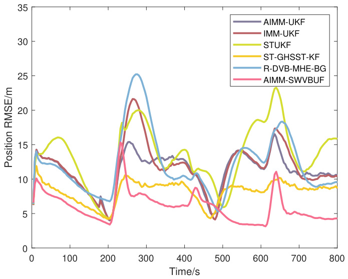
Figure 13.
Velocity RMSE of different algorithms in the simulation study.
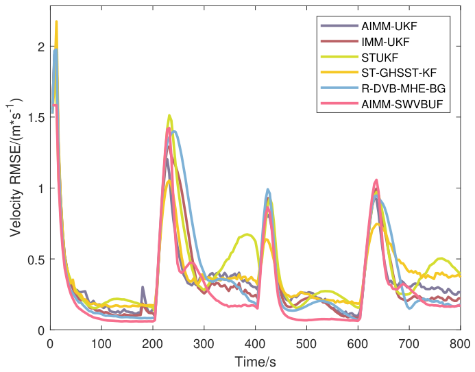
Figure 14.
Target trajectory and buoy layout in the lake trial.
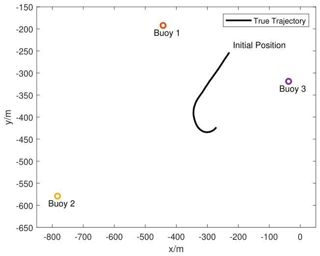
Figure 15.
Range measurements from the three buoys in the lake trial.
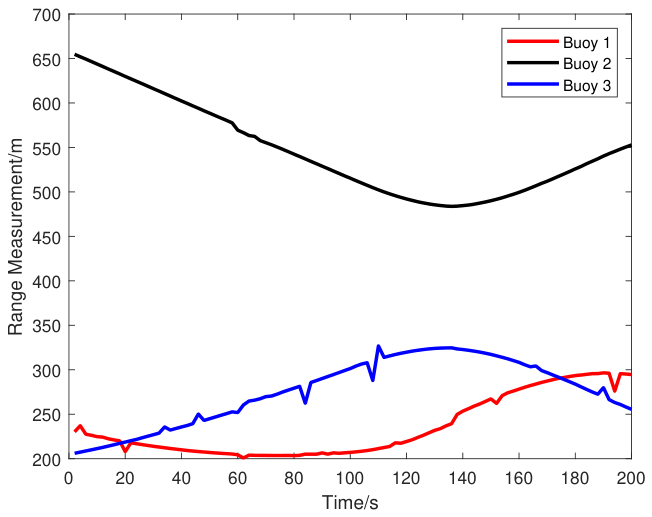
Figure 16.
Probability density functions of the measurement noise in the lake trial.
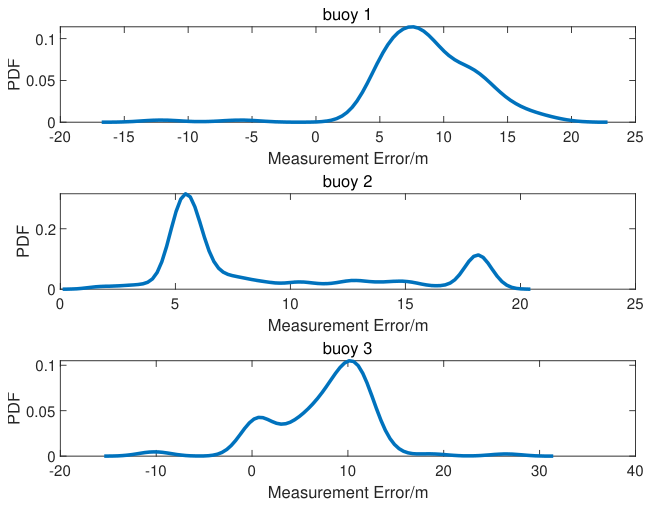
Figure 17.
Position estimation errors of different algorithms in the lake trial.
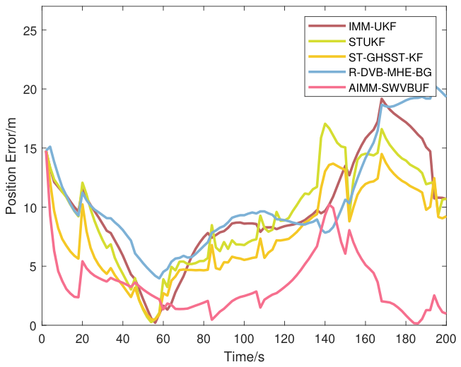
Figure 18.
Velocity estimation errors of different algorithms in the lake trial.
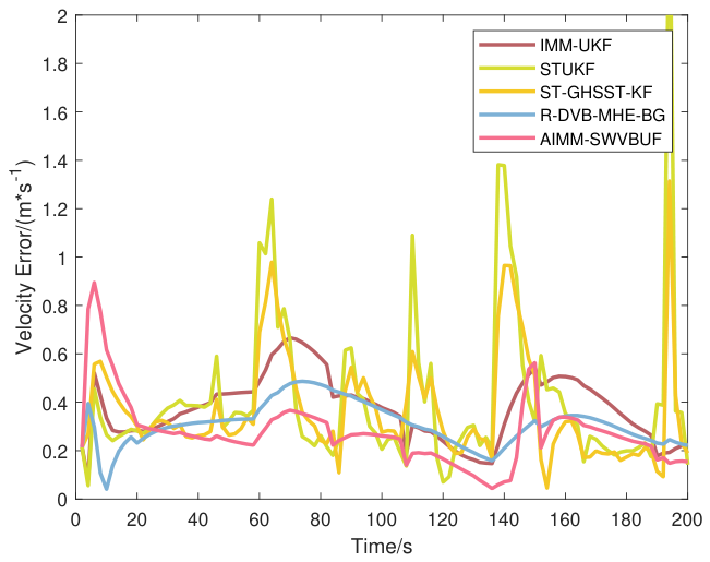

Table 1.
Floating-Point Computational Complexity of AIMM-SWVBUF.
| Step | × / + / − | Cholesky decomposition, Matrix inversion, Division and exponentiation |
|---|---|---|
| step1 | / | / |
| step2 | ||
| step3 | / | / |
| step5 | / | |
| step7 | ||
| step8 | ||
| step9 | ||
| step10 | / | / |
| step15 | / | |
| step16 | ||
| step18 | / | |
| step19 | / |
Table 2.
Target Motion Models over Different Time Intervals.
| Time/s | 1–200 | 200–400 | 400–600 | 600–800 |
|---|---|---|---|---|
| Motion Model | CV | CT () | CV | CT () |
Table 3.
Effect of Different c Values on the Performance of the Proposed Algorithm.
| Parameter c | Position ARMSE/m | Velocity ARMSE/(m/s) |
|---|---|---|
| 6.728 | 0.317 | |
| 6.263 | 0.299 | |
| 6.243 | 0.296 | |
| 6.091 | 0.295 | |
| 6.195 | 0.306 | |
| 6.265 | 0.315 |
Table 4.
Module configurations of the algorithms in the ablation study.
| Algorithm | Sliding-window parameter fusion | Adaptive process noise adjustment | Sliding-window MAP estimation |
|---|---|---|---|
| Baseline | × | × | × |
| w/o Fusion | × | √ | √ |
| w/o MAP | √ | √ | × |
| w/o Adapt | √ | × | √ |
| Full | √ | √ | √ |
Table 5.
Position and Velocity ARMSE of Different Algorithms in the Ablation Study.
| Algorithm | Position ARMSE/m | Velocity ARMSE/(m/s) |
|---|---|---|
| Baseline | 9.007 | 0.367 |
| w/o Fusion | 8.271 | 0.310 |
| w/o MAP | 6.905 | 0.296 |
| w/o Adapt | 6.747 | 0.318 |
| Full | 6.099 | 0.295 |
Table 6.
Position and Velocity ARMSE of Different Filters.
| Filter | Position ARMSE/m | Velocity ARMSE/(m/s) |
|---|---|---|
| AIMM-UKF | 11.182 | 0.367 |
| IMM-UKF | 11.630 | 0.368 |
| STUKF | 13.457 | 0.442 |
| ST-GHSST-KF | 8.038 | 0.370 |
| R-DVB-MHE-BG | 12.221 | 0.384 |
| AIMM-SWVBUF | 6.047 | 0.293 |
Table 7.
Average Running Time.
| Algorithm | Average Running Time (ms) |
|---|---|
| ST-GHSST-KF | 0.575 |
| R-DVB-MHE-BG | 4.495 |
| AIMM-SWVBUF | 0.425 |
Disclaimer/Publisher’s Note: The statements, opinions and data contained in all publications are solely those of the individual author(s) and contributor(s) and not of MDPI and/or the editor(s). MDPI and/or the editor(s) disclaim responsibility for any injury to people or property resulting from any ideas, methods, instructions or products referred to in the content. |
© 2026 by the authors. Licensee MDPI, Basel, Switzerland. This article is an open access article distributed under the terms and conditions of the Creative Commons Attribution (CC BY) license.
Copyright: This open access article is published under a Creative Commons CC BY 4.0 license, which permit the free download, distribution, and reuse, provided that the author and preprint are cited in any reuse.