

Submitted:
31 October 2026
Posted:
04 November 2026
You are already at the latest version
Abstract
In quantum mechanics energy is an observable, whereas time is a parameter; Pauli's theorem and the problem of time in canonical quantum gravity reflect this asymmetry. We define the time operator \( \hat{t}=\hat{x}/c \) and form, with the relativistic energy \( \hat{E}_R \), Einstein's constant \( \kappa \) and the time \( \hat{t}_0 \) in the rest system, operators of gravitational-field and curvature type, and derive their commutation relations, wave equations and spectra. The commutator \( [\hat{t},\hat{E}_R]=\tfrac{i\hbar}{c}\hat{v}_x \) is bounded with norm \( \hbar \) and is not a multiple of the identity, so Pauli's theorem is not contradicted. The sum \( c\,\hat{t}+\kappa\hat{E}_R \) is unitarily equivalent to the time operator and has a continuous spectrum. A postulated field equation, \( \hat{G}_0+\hat{\Lambda}=\kappa\hat{E}_R \), has the structure of Einstein's equation; for small velocities it becomes the Schrödinger equation of a particle in a homogeneous field. The metric tensor of this scalar model is not quantized. A metric operator is constructed from commuting position operators; in the vacuum sector it reproduces the Schwarzschild line element, which serves as a consistency test, and in general it is obtained only under an explicit correspondence condition, which is a postulate and not derived.
Keywords:
cause
; effect
; causal relationship \( k \)
; causality
; causation
1. Introduction
At the beginning of all things there is a quarrel. Energy presses forward, restless and full of strength, and wants to seize time and hold it fast. Time, however, flows on serenely and slips away from every grasp, as if none of this concerned it. The closer energy comes, the further time escapes, and the more firmly energy grips, the more fleeting time becomes. The two can never be grasped completely at the same moment; between them remains a remainder that cannot be removed. Yet it is precisely in this strife that they find each other, for each shows itself only through the other: energy becomes visible in time, and time in energy. Their opposition is thus at the same time their bond. Out of their being against each other grows a being with each other, and out of this being together something emerges that neither was alone, something new that preserves both within itself and that we call space. It is empty and yet filled, still and yet full of possibility. Like everything that is becoming see [1,2,3,4], it carries within itself what will one day emerge from it: the fields, the bodies and the whole world.
Physics has long recorded this tension but seldom given it a form. In quantum mechanics the energy of a system is an observable with a spectrum, whereas time is a parameter: the silent clock along which the wave function evolves, but never itself the outcome of a measurement. Space, by contrast, is represented by an operator whose spectrum is the whole real line. This asymmetry is not accidental. Pauli showed that no self-adjoint operator can be the canonical conjugate of a Hamiltonian that is bounded from below, and the same asymmetry returns in the canonical quantization of gravity as the problem of time. Whoever wishes to give the quarrel between energy and time a mathematical form must therefore decide how time is to be treated.
Here we follow a different path. Guided by the light-cone relation , we define the time operator by . Being a multiple of the position operator, it is self-adjoint with spectrum , and it is conjugate to the momentum and not to the energy. Its commutator with the relativistic energy, , is bounded, has the norm ℏ, and is not a multiple of the identity, so that Pauli’s theorem is not contradicted. Energy and time then stand to each other in two relations at once. They are opposed, because they do not commute, and they are united, because their sum forms a single operator with a continuous spectrum and explicit generalized eigenfunctions, which is unitarily equivalent to the time operator itself. The coupling constant is that of Einstein’s field equation, so that every term has the dimension of a curvature once it is divided by a volume V.
From this pair, and from the time in the rest system, we construct operators of gravitational-field type and of curvature type. We compute their commutation relations, derive Schrödinger-type wave equations in the time and in the energy representation, and determine their spectra. The operators are arranged in a table whose columns correspond to the terms of Einstein’s field equation, and which leads to a field equation of the same structure, . In it the term is an operator that is determined by the others, that can change in time but does not have to, and that has a continuous spectrum with an explicit eigenfunction for every value. The Ricci scalar then becomes an operator that contains the energy, and for small velocities the equation turns into the Schrödinger equation of a particle in a homogeneous field, with a force fixed by the speed of light and Newton’s constant.
One may read the construction as a statement about space: out of the opposition and the unity of energy and time something new arises that is neither of them, and in which both are preserved. We offer this reading as a theoretical possibility only (Remark 43); it is not a result of the paper. The results themselves are mathematical and are stated with proofs. In the operator model of Section 2 and Section 3 we do not quantize the metric or Einstein’s field equation. A metric operator is constructed only in Section 4, in the vacuum sector from commuting position operators and in general under one explicit correspondence condition, which is a postulate. The identification is a working hypothesis and not a consequence of standard quantum mechanics. The field equation is a postulate, and its proofs are given for one spatial dimension. We state these limits openly, because a structure whose boundaries are known is easier to build upon. The paper is organized as follows. Section 2 introduces the operators and the representations in which they are studied. Section 3 derives the commutation relations, the wave equations, the field equation and the Ricci scalar operator. Section 4 constructs the metric operator and discusses the quantization of gravitation under the correspondence condition. Section 5 discusses the scope and the limits of the approach, and Section 6 concludes.
2. Materials and Methods
This section contains the definitions and postulates only, arranged in five steps: geometry, probability, quantum mechanics, Einstein’s field equation, and the four fields of nature with the causal relationship k. All propositions, theorems, lemmas, remarks and proofs are collected in Section 3.
2.1. Geometry
The aim of this publication is to bring quantum theory and general relativity into a compatible mathematical language, and this requires common foundations. General relativity is built on the metric tensor, which generalizes the theorem of Pythagoras locally to , whereas quantum theory is built on operators in a Hilbert space. We therefore start at the most elementary level and define the elementary geometric entities, namely lengths, segments and angles, as quantum-mechanical operators. Lengths and segments become positive self-adjoint operators, angles become functions of them by the spectral calculus, and the theorem of Pythagoras becomes an operator identity. The segments and are complementary parts of the hypotenuse , so that and are probabilities; geometry and probability are thereby described by the same objects. We begin with the right isosceles triangle, because it is the simplest and most symmetric case (, probability ). This definition provides a common starting point and does not by itself establish a unification; the Lorentzian signature and the full tensorial form remain to be worked out.
Definition 1
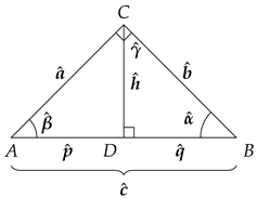
(Triangle). The right triangle with the right angle at C and the foot D of the altitude on the hypotenuse is described by the quantum-mechanical operators
and by the angle operators at A, at B and at C. The triangle is called isosceles if , equivalently . The relations between these operators are derived in Section 3 (Proposition 1).
Definition 2
(Operators of the right triangle). Let be a positive invertible operator, and let and be non-negative operators which commute with each other and with and satisfy . The legs and the altitude are defined by
and the angles by (spectral calculus)
2.2. Probability
Geometry and probability are not totally different. In the right triangle the squared ratios and are non-negative and add up to , so that the theorem of Pythagoras and the statement that two complementary probabilities sum to one express the same fact. They differ in content: geometry contains more than the two fractions (angles, orientation and, in general relativity, the signature), whereas the probability fixes only the fractions. For the Euclidean right triangle the two descriptions determine each other. For Lorentzian signature the Pythagorean sum carries a relative minus sign, and the fractions can leave the interval , as the example of dust shows.
Definition 3
(Expectation, probability and complementary operator). Let be a self-adjoint operator with (so that exists), and let be the expectation of in the state ψ for the event that manifests, which has the probability p, such that . The complementary event of comes into existence with the probability and has the expectation . The two events exclude each other and together exhaust ; no value 0 is assigned to the complementary event. The complementary event of may be, for example, a hidden variable that is not observed; no assumption about its locality is made here. is not the expectation value of the distribution of . Assume:
- (E1)
- is self-adjoint;
- (E2)
- and commute, i.e. their spectral projections commute;
- (E3)
- (this states that the probability p of the event lies between 0 and 1).
- The probability associated with isThe expectation of the complementary operator is , and .
Proposition 0
(Probabilities as effects). Under (E1)–(E3), and are bounded self-adjoint operators with
Proof.
By (E1), (E2) and the spectral theorem for commuting self-adjoint operators there are a measure space , a unitary map onto and real measurable functions x, e such that and become multiplication by x and e. Then and, by (E3), almost everywhere. Hence is multiplication by and by . Their sum is 1. □
Remark 1.
The pair is a two-outcome effect pair (a Positive Operator-Valued Measure (POVM)). For a normalized state ψ the numbers and lie in and add up to 1, so that no further probability distribution is required for this reading. The decomposition alone is an algebraic identity; the probability reading rests on (E1)–(E3). If (E3) fails, as for the fractions of the Lorentzian signature, p can leave and is then a quasi-probability. The expectation of a single event must be distinguished from the expectation value of the distribution of in a state: the choice would require by (E3), whereas always holds, so that would be guaranteed only in the boundary case. In an eigenstate of the event occurs with certainty, .
Remark 2
(Domains of the metric operator). The position operators commute, so functions of them, such as , are defined by the spectral calculus. The tensor contains the momentum operators , which do not commute with , and is unbounded at the origin. The operator is therefore defined on the dense domain , on which all products are defined; on it is symmetric. Essential self-adjointness is not claimed.
Definition 4
(Expectation value of the distribution of an operator). Let be a self-adjoint operator with the spectral measure , and let with . The distribution of in the state ψ is the probability measure on , and its expectation value is
For a density operator one has . The second moment is and the variance is .
Theorem 1
(Single event and distribution). Let (a self-adjoint operator, the observable), (an operator, the expectation of the single event “ manifests”) and (an operator, the probability of this event) satisfy (E1)–(E3) of Definition 3, and let (a state vector) with . For an operator write (a real number, the expectation value of the distribution of in ψ). Then
and
Define the complementary part of the distribution (a number) by
Then (the left side is defined as a remainder, the right side as , the expectation value of the operator of the complementary event), that is,
Proof.
By Theorem 2, . Taking the expectation value in and using linearity gives the first relation. In the joint spectral representation of Proposition 0, and with by (E3), which gives the inequality. The definition of together with the first relation gives . □
Remark 3.
The identity is trivial. Its content lies in the fact that is an operator and a number, so that only the expectation value can be subtracted, and that the remainder coincides with the independently defined in the state ψ. The weights are , a mean of weighted with the values x; it equals if is a multiple of or is.
Definition 5
(Second moment and variance). Under the assumptions of Definition 3, define the second moment of by
and the variance by
where denotes the product .
Definition 6
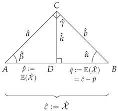
(Triangle in terms of the complementary decomposition). Let satisfy the assumptions of Definition 3 with . This is the situation of Definition 2 with
and the legs, the altitude and the angles of the triangle are defined by
Here is the second moment of Definition 5.
2.3. Quantum Mechanics
2.3.1. Wave Function
Definition 7
(Wave function and its complex conjugate). Let be a measure space whose points are the possible outcomes, at the parameter value t (for instance time), of an arbitrary quantity (for instance a position, a momentum, a price or a return, a measured value, a discrete label, a set of such variables, or a single number). For and μ the Lebesgue measure one has ; for a countable Ω and the counting measure the integrals below are sums. Let
be a measurable function, the (single) probability of the outcome , with
Let , , be an arbitrary positive real number (for instance or ), and let , , be an arbitrary real-valued measurable function. Constant functions are admitted, in particular . The wave function see [5,6,7,8,9,10,11] and its complex conjugate are defined by
Here is the non-negative square root, and are the complex phases. The probability of the outcome and the normalization follow from (25):
For a countable Ω, is the probability of the single outcome . Let be the probability that the outcome lies in a measurable set . For continuous Ω (Lebesgue measure μ) the probability of a single point is zero, and p is the probability density, i.e. the Radon–Nikodym derivative
which exists, conversely, for every probability measure P that is absolutely continuous with respect to μ () and is determined μ-almost everywhere. Thus is the probability of the outcome lying in . For the counting measure the two cases coincide, since and . The definition applies for each fixed t, and the normalization holds for every t. Where the dependence on t is not needed, is written X and is written p.
2.3.2. Position, Momentum, Relativistic Energy, Mass and Velocity
Definition 8
(Position operator). On the position operator is
which is self-adjoint.
Definition 9
(Momentum operator). On the momentum operator is
where is the relativistic mass operator and the relative velocity operator of Definition 10. These are functions of , defined from by the spectral calculus, and their product equals (Proposition 6(a)); the second equality in (29) is therefore a result and not part of the definition. The operator is self-adjoint and satisfies on .
Definition 10
(Relativistic energy, mass and relative velocity). Let be the rest mass and . Using the spectral calculus of , define
with . The operator is the relativistic total energy operator, the relativistic mass operator, and the velocity relative to the frame of the observer. The operator is defined by ; it is not defined through a commutator with .
2.3.3. Time Operator and the Operator
Time holds a curious place in quantum theory. Space is represented by an operator whose spectrum is the whole real line, whereas time is merely a parameter: the silent clock along which the wave function evolves, but which is never itself the outcome of a measurement. This asymmetry is not accidental. Pauli showed that no self-adjoint operator can satisfy with a Hamiltonian that is bounded from below, and the same asymmetry returns in the canonical quantization of gravity as the problem of time. Here we follow a different path. Guided by the light-cone relation , we define the time operator by . Being a multiple of the position operator, is self-adjoint with spectrum , and it is conjugate to the momentum, , not to the energy. Its commutator with the relativistic energy, , is not a multiple of the identity, so that Pauli’s theorem is not contradicted (Remark 11). The identification is a working hypothesis, not a consequence of standard quantum mechanics; its purpose is to explore a mathematical structure in which time and space appear on an equal footing, as observables.
Definition 11
(Time operator). Let be the speed of light. The time operator is defined by the operator relation
that is,
2.3.4. Time and Energy Representation
Definition 13
(Time and energy representation). Time representation. Let and with ; this is the position representation with , . In this representation
where functions of are defined by the spectral calculus. The operator generates time translations, .
Energy representation. Let and for , and let . The map
is unitary from onto , because . The index σ labels the two branches of the energy.
2.3.5. Operators of Gravitational-Field Type
Definition 14
(Operator families). For a constant let
with . Two values of λ are used.
- (i)
- Gravitational field ():of dimension .
- (ii)
- Einstein’s curvature terms (, where is a volume):where , and have the dimension of the terms in Equation (42), and itself has the dimension .
- The two families are proportional, .
Definition 15
(The operator ). Division of by c gives
and division by gives, with and ,
We define
The operator does not depend on V (equivalently, ). Its dimension is , the dimension of . It is the member of the family of Definition 14, , with and .
2.4. Einstein’s Field Equation
We use Einstein’s field equation see [13,14,15,16,17] in the form
where is the dimension of spacetime, the signature is in this general statement, , and . The terms , and have the dimension . The explicit examples of the Results (dust at rest, line element, Schwarzschild and Kerr–Schild form) use the signature ; this is a change of convention for these examples only and is stated again where it is used.
Postulate 1
(Negation law). Let be a self-adjoint operator with , (the entity), and let
with self-adjoint operators (positive part), (negative part) and (rest). The complementary operators are
The fractions are and , and likewise for and , so that
A part is pure if its complement vanishes: is pure if , that is , and is pure if , that is (for : ).
Definition 16
(Probability tensor of Einstein’s equation). Let (componentwise, no summation). For a tensor put
in particular
For an observer with one has , and and . This is the probability of Definition 3 with .
Definition 17
(Ricci metric and energy metric). In the notation of Proposition 6 (with ) put
the Ricci metric and the energy metric (the stress-energy tensor measured in units of ). They are metrics in name only: is non-degenerate only if is invertible, and its signature need not be Lorentzian.
Definition 18
(Normalization by the entity and the probability tensor). Let with the source at the origin, , and define the light-cone tensor of the time operators, which mirrors the energy-momentum tensor of Definition 19,
so that . Set
with , and the entity . The probability tensors are
Definition 19
(Metric operator from the negation law). Let a source of energy and momentum () be given, and let be the distance operator between the field point and the source. With define the energy-momentum operators of a point particle
and the metric operator
2.4.1. Field Equation for Operators
Definition 20
(Proper-time operator). Let (a multiple of the identity, ), the Lorentz factor, and the time of the observer’s frame. The time in the rest system is
Definition 21
(Operators of the table). Let and as in Definition 14, and
The operators of dimension
satisfy , and after division by V all operators of the table have the dimension :
The operator is not an operator of its own: it exists only through and , that is, through and .
Postulate 2
(Field equation). Let be the operator which represents the term Λ of Equation (42); is not assumed to be constant. The field equation is the operator equation
Definition 22
(Ricci scalar operator). The operator of the Ricci scalar is defined by
2.5. Four Fields of Nature, the General Field Equation and the Causal Relationship k
In this section a generally valid wave equation is formulated whose form does not depend on the meaning of the operators. Since the wave equation is built solely on the algebraic structure of the Negation law (Postulate 1), it is independent of the specific interpretation of the operators. The same mathematical structure can therefore be applied to quite different disciplines, from quantum field theory to financial mathematics and other complex systems, without deriving the equation anew in each case. The equation remains valid whether the operators stand for physical fields, prices or other quantities. In this way the approach connects an abstract algebraic structure with applied science without being tied to the conventions of a single discipline. The generality claimed here concerns this structure; what the operators represent, and whether the postulate holds for a given application, has to be established separately in each case. The index R denotes the system observed from the standpoint of special relativity by an external (relativistic) observer. In this section is the entity (denoted in Postulate 1); all operators of this section carry calligraphic letters (), so that they do not coincide with the operators of Definition 18 and of Remark 21; the operator is defined below as the generalization of the operator of the field equation (Remark 24) and is distinguished from it by the index R; it is not the cosmological constant of Equation (42); the volume V is not an operator of this section. Let be a dense subspace of the Hilbert space which lies in the domain of every operator below and is mapped into itself by each of them; all operator equations hold on .
Definition 23
(Operators of the general wave equation). Let be four symmetric operators (the elementary fields; their structure is left open), and let be symmetric operators (meaning left open) with
Thus and are two pairs of a part and its complement with respect to the entity in the sense of Postulate 1 (with ). Define
Definition 24
(Four-field structure). The operators of Definition 23 are built from the elementary fields as the row, column and total sums of the scheme ,
Definition 25
(The causal relationship k in a state). Let (62) hold with (symmetric, not necessarily commuting), and let , , be a state. Put and likewise ; by linearity
are the expectation values of . Define the scale (assumed), the deviation from the independent value , and, with the probability map of Theorem 2,
If the fields are multiplication operators by functions on and ψ is the wave function of Definition 7 (whose outcome variable is written here), then and likewise for ; the phase y does not enter.
Definition 26
(The operator for commuting fields). Let commute pairwise and let be positive and invertible. Define
By Proposition 6(b), for commuting fields. On a joint eigenvector with the eigenvalues the operator takes the value , which is ; for non-commuting fields it is not defined.
Definition 27
(Necessary condition). Let (62) hold with . The necessary condition (conditio sine qua non) is
The wave function Ψ of a state ψ satisfies the necessary condition if, with , (Postulate 1),
Since , in the commuting case this is equivalent to : without the cause there is no effect in the state ψ. The operator condition implies (67) for every Ψ; (67) is the condition for a given Ψ. In the situation of Proposition 8 it is the implication , that is, almost surely. If is the multiplication operator by on (Definition 25), the condition reads , that is, μ-almost everywhere on .
Definition 28
(Probability of the necessary condition and of its violation). Let (62) hold with and , (Postulate 1). Define, with the symmetric form of Theorem 2,
so that the two complement each other,
The first quantity is the probability that the necessary condition holds, the second ( in the scalar case) is the probability, or the extent, to which the necessary condition is not present. For a state ψ, Ψ its wave function and (so that ), let
which again add up to 1.
Definition 29
(Defect of necessity). In the situation of Definition 28 let
The value () is the necessary condition of Definition 27; a value such as or means that the fraction or of the weight of the state is “effect without cause”, that is, the extent to which the necessary condition is not present.
Definition 30
(Sufficient condition). Let (62) hold with . The sufficient condition (conditio per quam) is
The wave function Ψ of a state ψ satisfies the sufficient condition if, with , (Postulate 1),
Since , in the commuting case this is equivalent to : whenever the cause is present, the effect is present in the state ψ; there is no cause without effect. The operator condition implies (74) for every Ψ; (74) is the condition for a given Ψ. In the situation of Proposition 8 it is the sufficient condition in its logical form , that is, almost surely. If is the multiplication operator by on (Definition 25), the condition reads , that is, μ-almost everywhere on .
Definition 31
(Probability of the sufficient condition and of its violation). Let (62) hold with and , (Postulate 1). Define, with the symmetric form of Theorem 2,
so that the two complement each other,
The first quantity is the probability that the sufficient condition holds, the second ( in the scalar case) is the probability, or the extent, to which the sufficient condition is not present. For a state ψ, Ψ its wave function and (so that ), let
which again add up to 1.
Definition 32
(Defect of sufficiency). In the situation of Definition 31 let
The value () is the sufficient condition of Definition 30; a value such as or means that the fraction or of the weight of the state is “cause without effect”, that is, the extent to which the sufficient condition is not present.
Definition 33
(Condition of exclusion). Let (62) hold with . The condition of exclusion (conditio exclusionis) is
The wave function Ψ of a state ψ satisfies the condition of exclusion if, with , (Postulate 1),
Since , in the commuting case this is equivalent to : in the state ψ the cause and the effect exclude each other; they never occur together. The operator condition implies (81) for every Ψ; (81) is the condition for a given Ψ. In the situation of Proposition 8 it states that does not occur, that is, almost surely. If is the multiplication operator by on (Definition 25), the condition reads , that is, μ-almost everywhere on .
Definition 34
(Probability of the exclusion and of its violation). Let (62) hold with and , (Postulate 1). Define, with the symmetric form of Theorem 2,
so that the two complement each other,
The first quantity is the probability that the condition of exclusion holds, the second ( in the scalar case) is the probability, or the extent, to which cause and effect occur together, that is, to which the condition of exclusion is not present. For a state ψ, Ψ its wave function and (so that ), let
which again add up to 1.
Definition 35
(Defect of exclusion). In the situation of Definition 34 let
The value () is the condition of exclusion of Definition 33; a value such as or means that the fraction or of the weight of the state is “cause and effect together”, that is, the extent to which the condition of exclusion is not present.
Definition 36
(Condition of equivalence). Let (62) hold with . The condition of equivalence (conditio per quam et sine qua non), that is, the necessary and sufficient condition, is
the conjunction of the necessary condition (Definition 27) and the sufficient condition (Definition 30). The wave function Ψ of a state ψ satisfies the condition of equivalence if, with , (Postulate 1),
Since , the first condition is equivalent to , and in the commuting case to : the cause is present exactly when the effect is present. The operator condition implies (88) for every Ψ; (88) is the condition for a given Ψ. In the situation of Proposition 8 it states that almost surely. If are multiplication operators by on (Definition 25), the condition reads μ-almost everywhere on .
Definition 37
(Probability of the equivalence and of the pure opposition). Let (62) hold with and , (Postulate 1). Define, with the symmetric form of Theorem 2,
so that the two complement each other,
The first quantity is the probability that cause and effect are equivalent, the second ( in the scalar case) is the probability, or the extent, of the opposition, in which the cause occurs without the effect or the effect without the cause. The first quantity is the probability that cause and effect are equivalent: the cause is accompanied by the effect (), and the non-cause by the non-effect () (co-occurance of events). The second ( in the scalar case) is the probability, or the extent, of the opposition, in which the roles are interchanged: the presumed cause is accompanied by the non-effect (), and the presumed non-cause by the effect (). In the pure opposition the non-effect is the main effect of the presumed cause and the non-cause is the main cause of the effect, and (Proposition 8). For a state ψ, Ψ its wave function and (so that ), let
which again add up to 1.
Definition 38
(Defect of equivalence). In the situation of Definition 37 let
where is the defect of sufficiency (Definition 32) and the defect of necessity (Definition 29), . The value () is the condition of equivalence; a value such as or means that the fraction or of the weight of the state is “cause without effect or effect without cause”.
Definition 39
(Condition of disjunction). Let (62) hold with . The condition of disjunction (logical or) is
The wave function Ψ of a state ψ satisfies the condition of disjunction if, with , (Postulate 1),
Since , in the commuting case this is equivalent to : in the state ψ at least one of the cause and the effect is present, the case that neither is present does not occur. The operator condition implies (95) for every Ψ; (95) is the condition for a given Ψ. In the situation of Proposition 8 it is the statement almost surely, that is, almost surely. If is the multiplication operator by on (Definition 25), the condition reads , that is, μ-almost everywhere on .
Definition 40
(Probability of the disjunction and of the joint denial). Let (62) hold with and , (Postulate 1). Define, with the symmetric form of Theorem 2,
so that the two complement each other,
The first quantity is the probability that cause or effect (or both) is present, the second ( in the scalar case) is the probability, or the extent, to which neither of them is present. The second is the joint denial (“neither U nor W”, the logical NOR); it is denoted by ∪ with a vertical bar. For a state ψ, Ψ its wave function and (so that ), let
which again add up to 1.
Definition 41
(Defect of the disjunction). In the situation of Definition 40 let
The value () is the condition of disjunction of Definition 39; a value such as or means that the fraction or of the weight of the state is “neither cause nor effect”, that is, the extent to which the disjunction is not present.
3. Results
This section contains the propositions, theorems, lemmas, remarks and proofs which follow from the definitions and postulates of Section 2.
3.1. Relations of the Right Triangle
Proposition 1
(Relations of the right triangle). Let the operators be defined as in Definition 2. Then
and, if is invertible,
If the triangle is isosceles, , then
Proof.
All operators are functions of the commuting operators , so that the spectral calculus applies and they commute. Since and , one has , so that the angles of Definition 2 are well defined with values in .
(101) is the square of (4). Further , which is (102). By definition and because on ; hence and (103) follows with . The squares (105) and (106) are the definitions. Since commutes with , , and analogously , which gives (104) and (107). Then , and if is invertible. For one has , hence , , and therefore . □
3.2. Complementary Decomposition, Variance and Probability
Theorem 2
(Complementary decomposition of an observable). Under the assumptions of Definition 3,
and .
Proof.
By (??),
Since and commute, . Hence
which gives . Finally, . □
Remark 4.
In Theorem 2 the symbol denotes the value defined by (??), which equals ; the theorem is the rearrangement of this definition. If is taken as an operator and is applied to it literally, then , and the relation holds only if ; for an idempotent this forces and . The probability reading requires .
Theorem 3
(Variance of the complementary decomposition). Under the assumptions of Theorem 2,
If , then .
Proof.
Since and commute, , hence by (14). Then
because by Theorem 2. Inserting and gives the second form. If , both factors are non-negative and commute, so their product is non-negative. □
Remark 5
(Comparison with the usual variance). The usual variance of a random variable X is , where is computed from the whole distribution of X. In Definition 5 the second moment is instead fixed by and the single probability . The two definitions coincide for a quantity that takes the value x with probability p and the value 0 otherwise: then , and with . This is the situation of the event fields . In an eigenstate of one has , and both variances vanish. For a quantity with more than two values, in general, and Definition 5 is then a special case that does not replace the usual variance.
Theorem 4
(Probability and variance). Under the assumptions of Theorem 2, let be invertible. Then
that is, in the scalar notation.
Proof.
It is
and therefore
Multiplying by (all operators involved are functions of and and commute) gives
With and the first term is
that is, it is the probability itself and not a new quantity. Hence
and the probability is also determined by
Since (Theorem 2), also . □
Remark 6.
The smaller , the closer is to , and holds if and only if . If is not invertible, the quotient is not formed and no statement is made; no rule for is used, but it appears to be necessary that 0/0 = 1.
Theorem 5
(Euclid’s theorems for the complementary decomposition). Under the assumptions of Theorem 2, put , , , , and with . Then
Proof.
is Theorem 2. By Theorem 3, and . By definition . Finally . □
Remark 7.
These are the relations of the right triangle with hypotenuse c, hypotenuse segments , legs and altitude h (Euclid’s leg theorem and altitude theorem, and the theorem of Pythagoras). For commuting operators, in the spectral representation, p and q are real numbers and the geometry is literal. For non-commuting fields the non-commutativity is carried by the operators and . These basic relationships of algebra could be useful for a description of general relativity by quantum-mechanical operators.
Theorem 6
(Geometry and probability). Let satisfy the assumptions of Theorem 2 with . Consider the right triangle with hypotenuse , hypotenuse segments and , so that , and legs with and ; here a is the leg opposite to the angle α and p is the segment adjacent to a. Then
and hence
with (square roots in the spectral calculus).
Proof.
By Theorem 2, , that is, . Multiplying by gives
where and . Define
so that . Since and , ,
by (Theorem 2). Taking square roots, which is possible because , gives the boxed formulas. □
Remark 8.
Geometry and probability are closely related: the squared sine and cosine of the angle α are the two complementary probabilities and , in the form of the Born probabilities of a two-outcome measurement. Moreover , and by Theorem 5.
Remark 9
(Theoretical significance). Theorems 5 and 6 show that the theorem of Pythagoras, and with it the relations of the right triangle, can be expressed entirely in terms of the complementary probabilities and : the squared sine and cosine of an angle are probabilities, and the squared lengths of the legs are the corresponding fractions of the squared hypotenuse. This is of strategic importance, because the theorem of Pythagoras is the foundation of the metric tensor of general relativity, which generalizes it locally to . Consequently, it is plausible that the metric tensor—and with it the full geometry of general relativity—admits an equivalent description in probabilistic terms, preserving all structural information. The decomposition of the Ricci tensor into the four fields and the state-based causal relationship would then belong to one and the same probabilistic language. Geometry, probability and the quantum-mechanical operator calculus would no longer be separate descriptions but different readings of the same objective reality. The present results establish this only for the algebraic structure; the Lorentzian signature, in which the Pythagorean sum carries a relative minus sign, and the full tensorial form remain to be worked out. We regard the construction of the metric tensor from the probabilities as the natural next step of scientific progress.
Proposition 6
Proof.
By Theorem 2, , and commute with , so that Proposition 1 applies. Since commutes with and , , which gives (132) and (133); (134) follows with Theorem 3, and (135), (136) are Theorem 5. Because and , the angle relations (137)–(143) are (103)–(109), and Theorem 6 gives the sine and cosine. For one has . □
3.3. Quantum-Mechanical Operators
Remark 10.
The definition (25) is as general as possible in the following sense.
- (i)
- Probability and phase are separated. The factor carries the probability of the outcome , and the unimodular factor carries the phase. Apart from measurability, no structure is assumed about p or y, and none about the meaning of . The definition is therefore purely structural and applies in physics, finance, medicine, or to elementary numbers alike.
- (ii)
- Every pure state has this form. Let with . Set and write with a measurable phase θ (arbitrary where ). For any admissible b, the choice reproduces ψ exactly. A global phase corresponds to the shift .
- (iii)
- The conjugate is the inverse phase. Since , the pair is the standard pair of a wave function and its complex conjugate. The identification of the probability with the squared modulus (Born rule) is built into the definition. If a weight with is given instead of a normalized probability, one sets .
- (iv)
- The choice of the base is immaterial. The pairs and with define the same wave function; e.g. with y and with . For the phase is trivial and . A constant gives only a global phase.
- (v)
- Special cases. Single number: , gives , and for . Two outcomes: , , give , . Countable outcomes: with . Continuous outcomes : . Plane wave: constant on a finite volume V, and give up to a constant phase.
- All quantities that depend only on are independent of b and y; the phase y becomes relevant only for interference or superposition.
Proposition 6
(Momentum, energy and velocity).
- (a)
- on , and .
- (b)
- is self-adjoint with purely continuous spectrum . The operator is bounded, self-adjoint and injective, with and .
- (c)
- On one has, in this order of the factors,
Proof.
All operators are functions of the self-adjoint operator , which has purely absolutely continuous spectrum . By the spectral calculus the identities in (a) reduce to and with , , . The range of E is and each level set of E is finite, so that has no eigenvalues. Moreover with for , and only for , which gives (b). (c) follows from by multiplication with from the right. □
Proposition 6
(Time operator).
- (a)
- is self-adjoint on , and .
- (b)
- is unbounded and has the purely continuous spectrum ; it has no eigenvalues in .
- (c)
- On one has and .
Proof.
is a non-zero real multiple of the self-adjoint operator with the same domain, hence self-adjoint, and . If , then almost everywhere, hence . (c) follows from . □
Remark 11.
- (i)
- Relation to Pauli’s theorem. The operator is proportional to the position operator. It is not the canonical conjugate of the Hamiltonian , which is bounded from below: (Lemma 6(a)). Pauli’s theorem, which excludes a self-adjoint with for a Hamiltonian bounded from below, is therefore not contradicted.
- (ii)
- Status. The identification (31) corresponds classically to , the propagation of a light signal. It is a working hypothesis and not a consequence of standard quantum mechanics, in which t is a parameter.
Remark 12
(Several space dimensions). For on the time operator can be written in a uniform way as
where is a vector of commuting self-adjoint operators and is self-adjoint; gives Definition 11. With and one has , with , hence and . Moreover with , and commutes with the momenta orthogonal to the direction ; on each fibre of fixed orthogonal momentum the operators therefore have the one-dimensional form with a replaced by and by . This indicates how the one-dimensional results extend; it is not proved here. Powers such as are not components of a tensor, and a tensor-valued time operator is not worked out.
Remark 13
(Tensor of time operators and the metric). The vector of commuting self-adjoint operators contains the full information of the n directions; the sum of Remark 12 is the projection onto the direction and is needed only if a single scalar time operator is wanted.
A matrix requires a definition of , because position carries one index. The choice gives a matrix of rank one, , which cannot be a metric. The division has the dimension , whereas is dimensionless.
A dimensionless operator of metric type follows from the operators and of Definition 18 (with in place of ). With the Schwarzschild coefficient reads
on , where V cancels. This is a potential-type quantity. A field-type quantity is obtained from its derivative, which in the present formalism is a commutator with the momentum,
in analogy with the Christoffel symbol . The ordering and the domain near are not worked out.
Proposition 6
(The operator ).
- (a)
- is self-adjoint on , and .
- (b)
- is unbounded with purely continuous spectrum , and it commutes (strongly) with and .
- (c)
- On one has .
Proof.
As for Proposition 6, with replaced by ; , and are real functions of the self-adjoint operator . □
Remark 14
(Dimension and status of ). With and one has . The gravitational field has the dimension , and the gravitational potential Φ the dimension . Field and potential are not identical, since g is the gradient of Φ. The operator is therefore not itself the gravitational field. The relation can determine the gravitational field only under the following conditions.
- (i)
- A constant of dimension is included, .
- (ii)
- For the potential of a cosmological constant Λ and along light rays, , one hasi.e. , which has the required dimension.
- Under these conditions the gravitational field is determined by up to the constant and is represented by the operator . We do not claim that this identification holds for the gravitational field in general. The definition of implies no dynamical equation; the identification is a working hypothesis and not a consequence of Einstein’s field equation.
Lemma 6
(Time translations and energy representation).
- (a)
- For every smooth function g (real or complex) with polynomially bounded derivatives, maps into itself and
- (b)
- In the energy representation, acts as the multiplication by E, as the multiplication by , and on
- (c)
- In the energy representation, .
Proof.
(a) By the translation property, , hence . Superposition of the exponentials gives the claim for all functions g of in the spectral calculus.
(b) and act on as the multiplications by and ; at these are E and . Moreover, . With one has and therefore . With this is . For , is continuous at , i.e. .
(c) . □
3.4. Einstein’s Field Equation as a Negation Law
Proposition 6
(Complementarity of the parts). Let be as in Postulate 1. Then
- (a)
- , , , and
- (b)
- The complement is an involution, ; the complement of the empty part is the entity, , and . The only self-complementary part is , with . The statement would require and is excluded by .
- (c)
- The fractions commute, , whereas the parts commute if and only if they commute with the entity: . The non-commutativity of the parts is therefore measured exactly by the single operator , and not by an inequality. If ψ is an eigenvector of or of , then (see the proof), and the parts admit a joint spectral resolution, that is, simultaneously sharp values in a complete system of states, if and only if .
- (d)
- The product form of the law holds up to a commutator,
- (e)
- Let be a generator with and . Then : the sum is conserved, and a transition between the part and its complement takes place if and only if .
- (f)
- If , then , and the degree of mixing in a state ψ is ; it vanishes for all ψ if and only if is a projector (the part and its complement exclude each other).
Proof.
(a) gives ; the sum is ; . (b) Direct. (c) commutes with ; ; for one has , so that , and likewise for since ; the joint spectral resolution exists if and only if the operators commute. (d) . (e) and . (f) preserves the order, and . □
Proposition 6
(Probability of a part and the wave function). Let ψ be a state with , let , and define the probability associated with the part by
that is . Then
- (a)
- , hence .
- (b)
- With one has andthe share of the expectation value of the entity which is carried by the part.
- (c)
- , , , , and for the three probabilities add up to 1.
- (d)
- If and have a common eigenbasis with the eigenvalues and , thenand if is a projector, is the Born probability of the subspace of .
- (e)
- In the energy-momentum representation , for , and in the time representation , where ,For (Remark 16) this is .
Proof.
(a) By definition . (b) is bounded and self-adjoint, so and . (c) From follows ; the other relations follow from (a) and . (d) . For a projector . (e) Spectral theorem for , with the Fourier transform of . □
Remark 15
(Status of the probability). The relations (a)–(e) are identities. That is the probability of the part is the interpretation of the Negation law. It agrees with the Born rule whenever is a projector (in particular in the classical case , Proposition 6) and is the Born rule for the effect in the general case, where is a generalized measurement. That this assignment is the only possible one is not shown.
Proposition 6
(Classical logic as a special case). Let the entity be the unit, (in the scalar case ), and let be a projector, , with the eigenvalues 1 (true) and 0 (false). Then and
- (a)
- , , , ; in operator form , exact because (Proposition 6(d)).
- (b)
- (excluded middle), (non-contradiction), , and .
- (c)
- All operators commute, ; with and one has , so that the law contains the Boolean algebra of classical logic.
- More generally, for an arbitrary entity the part is classical if and only if is a projector which commutes with ; then , and the mixing of Proposition 6(f) vanishes. A non-projector or gives the non-classical case: remains valid, but non-contradiction holds only in the weakened form .
Proof.
(a),(b) For a projector , and . (c) . For the general statement, commuting with gives and , while if and only if is a projector. □
Remark 16
(Application: the factor ). Let , , and
With the fractions are
that is and . The decomposition is the Legendre relation with and . Both parts are functions of , so ; with respect to the time operator they are complementary,
The choice is motivated by and is not fixed by Postulate 1; the choice gives instead.
Proposition 6
(Probabilities from the normalized Ricci tensor). Let and define the dimensionless tensors
Equation (42) then reads . Division by , componentwise, gives
so that for . These are the componentwise fractions of Postulate 1 with the Ricci tensor as entity; contracted with they give (Proposition 6).
Example: dust at rest (, , u the rest frame, signature ):
The time component lies outside (quasi-probability, since and have the same sign but has the opposite sign); the three space components give and (pure geometry).
Proof.
Divide by . For dust, , , : , , , . □
Remark 17.
The division is componentwise and therefore frame dependent, and it is undefined where (for instance for a source at rest); the contraction with a four-velocity is the covariant version.
Remark 18
(Caution). The following relations are offered as a possible path towards a probabilistic formulation of Einstein’s theory, not as a result. There are good reasons for considerable doubt, and the reader should keep them in mind.
- (i)
- The relations are algebraically equivalent to the Einstein equation itself; they contain no new physical content and no new prediction.
- (ii)
- They are circular in the following sense: and R are functions of and its derivatives, so that the metric is not obtained from the probabilities but remains the solution of the field equation.
- (iii)
- The componentwise quotient of two tensors is not covariant; only the endomorphism form is.
- (iv)
- The reading of the quotients as probabilities requires , that is, conditions on the signs of and of the eigenvalues of , which are not guaranteed for Lorentzian signature (dust, Proposition 6).
- (v)
- The quotients are of the form where , that is, precisely for important vacuum solutions. In the system adopted here the rules and are used formally (Remark 35); the quotient occurs in for with a non-vanishing numerator. The consistency of these rules with the relations of this section, in particular with the complementarity at the points , where gives , is not examined here and is left to later work.
- (vi)
- The quantities are fractions of curvature and not frequencies of measurement outcomes; that they obey the Born rule for some state is not shown.
- (vii)
- The non-linearity of general relativity resides in and is not removed by the reformulation.
- Whether the path leads to a probabilistic description of general relativity without loss of information has to be decided by later work.
Proposition 6
(Probabilities from the Ricci metric). Let the Einstein Equation (42) hold.
- (a)
- , and for (componentwise, no summation)so that and : in units of the Ricci metric, the metric tensor and the energy metric are the two complementary fractions of Proposition 6. Moreover for .
- (b)
- (Covariant form.) If is invertible, the endomorphisms and satisfy . With , and , the Einstein equation is the relation of Theorem 2; is a multiple of the identity and commutes with , , , and by Theorem 3, .
Proof.
(a) Divide by , and the result by ; the last formula is the quotient of the two fractions. (b) Raising an index gives , which is ; a multiple of the identity commutes with every operator, so that Theorems 2 and 3 apply. Further , hence and , and by Theorem 2. □
Remark 19
(Geometrization of the energy-momentum tensor). For the relation
expresses the energy-momentum tensor completely through the metric , the scalar and the dimensionless ratio of the two complementary probabilities. The ratio is not an independent quantity as long as only Equation (42) is used, since it is by definition ; Equation (169) is a rewriting of the field equation, not a new equation. It gains content as soon as the ratio is fixed by a matter model (for example for a perfect fluid with ). Under this condition, the following consequences arise.
- (i)
- Matter as a modulation of the metric. Matter is no longer an additional field next to the geometry: is the metric , rescaled by a scalar and a ratio of probabilities. The distinction between “geometry” on the left and “matter” on the right of Einstein’s equation becomes a distinction between the two fractions and of one and the same quantity .
- (ii)
- Reduction of the unknowns. The field equation becomes an equation for and the ratio alone; no independent source field has to be specified. The vacuum corresponds to , and the pure cosmological-constant case to a constant ratio, that is, to in the perfect-fluid case.
- (iii)
- Energy conditions become conditions on probabilities. Since , a sign or bound of is a statement about the range of : the interval is possible exactly if , whereas dust (, ) leaves it. Energy conditions thus receive a probabilistic reading.
- (iv)
- Equation of state from geometry. For a perfect fluid, follows from , so that the equation of state is read off from the metric and the curvature, that is, a thermodynamic quantity becomes a geometric one.
- (v)
- Conservation law as a constraint on the ratio. The condition is, by , a condition on the ratio and on . If the ratio f does not depend on , it reads , so that is constant. Admissible matter models are thus restricted by geometry alone.
- (vi)
- A single object to be quantized. In the operator formulation, only the metric (and the probabilities p as operators) has to be quantized; then follows by Equation (169) and inherits its operator character. This is the connection to the program of describing general relativity by quantum-mechanical operators.
- (vii)
- A possible operator form. In the scalar model of Definition 18, , and , with , and . If , thenand, if in addition is invertible,which is the operator form of Equation (169), with the ordering fixed by . Equations (170) and (171) are a rewriting of and are therefore consistent with the total relativistic energy of Definition 10: with the Hamiltonian , the spectrum, the commutator and the Heisenberg equation are unchanged.
- These statements hold under the stated assumptions, namely and a ratio fixed independently of Equation (42). They do not replace a dynamics for the matter fields, and the scalar model is not touched by them.
Remark 20
(Negative quantities). The decomposition is linear: if , then . A world of negative quantities, with and both parts , leads under today’s rules, as long as negative divided by negative is positive, to the same probabilities, , in , and not to negative probabilities. There is some slight evidence that negative divided by negative remains negative. In this case one would have , that is, negative probabilities would have to be considered, and the sum of the two parts would be instead of 1. The reader should be prepared for this case; it is not decided here. The probability reading in requires, in any case, that and have the same sign as ; for parts of opposite sign, p lies outside , and this case is not covered by the reading.
Proposition 6
(Negation law for the probability tensor).
- (a)
- The relation is the definition , and .
- (b)
- (Postulate 1), , and in every state ψ the probabilities and satisfy (Proposition 6). For , .
- (c)
- and .
- (d)
- To first order in one has , (V cancels), and the metric operator of Definition 19 isthat is, up to the factor and the trace reversal the metric perturbation is the probability tensor of the energy part.
- (e)
- In the commuting (classical) limit, for a source at rest, and ; the self-complementary point lies at .
Proof.
(a) and . (b) and give and ; the rest is Proposition 6 and 6. (c) and . (d) gives ; insert this into Definition 19. For the source at rest, and . (e) The classical limit of (b) with , . □
Remark 21
(Limits). The equation is an identity by the definition of and carries no dynamical content; the content lies in the normalization and in the negation law. With the time operator itself, whose spectrum is , has the spectrum and the fractions have no probability reading; the positive operator is therefore used. Only the component 00 satisfies , the components and are fractions of a tensor entity and are not probabilities. The symbol is used in the article for , so the entity is denoted here.
Proposition 6
(Properties of the metric operator).
- (a)
- Dimension. All are dimensionless, since and are lengths.
- (b)
- Negation law. and . These are the parts and of Remark 16: the entity is decomposed into the trace and the spatial stress, with the fractions and .
- (c)
- Source at rest (). With ,where is the negation law for the entity (on spectral subspaces , , as required by Postulate 1) with the parts and . For this is the weak-field metric , with .
- (d)
- Exterior and interior. holds if and only if . Then is an effect and Proposition 6 applies. Where has negative expectation values () , the signature changes, and the part is negative; the probability reading is not available there.
- (e)
- Moving source. For , and .
- (f)
- Field and potential. The derivative of the potential-type operator is a commutator, , and gives the field-type operators (Christoffel symbols).
Proof.
(a) Dimension count. (b) , and Remark 16. (c) For : , , hence and . (d) and in the form sense. (e) . (f) . □
Remark 22
(Limits of the proposal). The definition is the linearized, quasi-static metric with the instantaneous Green function and no retardation; it is not a solution of Einstein’s equation beyond the weak field. The operator is the distance between the field point and the source, and the orderings are needed because and the source momentum do not commute. The relation splits the potential, ; whether this split has a physical meaning is open.
Proposition 6
(Einstein’s equation as a negation law). Let be a four-dimensional metric () with signature , its Ricci tensor, R the Ricci scalar. (The Equation (42) above is stated for the signature ; under the tensors and and the product are unchanged, whereas changes sign, so that here.) Let the sign convention be such that
For an observer with the four-velocity , , define the scalars , and the fractions of the entity ,
Then
- (a)
- is Einstein’s equation divided by the entity , and follows from the metric by differentiation once is known: .
- (b)
- For a perfect fluid at rest with the pressure and : , and
- (c)
- Let , , and consider the component of a fluid at rest. For both fractions lie in if and only if . Radiation and every traceless source (, , ) give , (pure matter part). The value is reached for (speed of sound c). Dust () gives , , so the probability reading is lost for the time component, although dust satisfies all energy conditions. For one has and both quotients are of the form . For the quantity is negative (the strong energy condition is violated, gravity is repulsive), and then and ; both fractions leave , in analogy to the negative sector of Remark 20. For the fractions remain in and tend to 0 and 1, respectively, as ; such values are excluded physically by causality (), not by the probability reading.
Proof.
- (a)
- Divide the field equation, contracted with and , by .
- (b)
- , ; the trace of the field equation for gives , and .
- (c)
- Since for , one has , and is equivalent to . In this range also lies in . For one obtains , , and for one obtains ; the condition is equivalent to , which is the causality bound and not a condition for the probability reading. For one has and therefore and . Dust gives , . □
Remark 23
(Scalar model and circularity). In the scalar model of the table, , and , the field equation reads , which is the identity of Definition 18; the fractions of Proposition 6 correspond to and . If the metric is defined from the probability tensor by Proposition 6(d), , the linearized Einstein equation is satisfied by construction because uses the Green function ; the equation is then an input and not a consequence. The metric tensor and Einstein’s equation are used here classically and are not quantized.
3.5. General Field Equation and the Four Fields
Proposition 6
Proof.
(a) Subtract from . (b) Apply (a) to . (c) . (d) Insert the definitions. □
Remark 6
(Status). Proposition 6 is an algebraic identity: it contains no dynamics and follows from the Negation law alone. The field equation of the article has this form with and . The dynamical content enters only through a realization of the operators, as in Proposition 6.
Proposition 6
(Commutators and quantization). Put , , . Under (60) and (61)
All commutators of the operators of Definition 23 are therefore linear combinations of and vanish if and only if these three do. The non-commutativity is measured by these three operators themselves, and no uncertainty inequality is used (Proposition 8(d)); in particular, for each pair, in every state ψ that is an eigenvector of or of , in agreement with Proposition 6(c).
Proof.
Write , , , and expand with bilinearity and antisymmetry; for example . For an eigenvector of one has , hence , and likewise for an eigenvector of . □
Remark 25
(Quantization). Relations (60) and (61) are linear. If are the classical phase-space functions of , the linear relations pass to the operators without an ordering ambiguity, and the three basic brackets are fixed by the correspondence , which is exact for at most quadratic functions. Together with Proposition 6 this gives the quantization of all operators of Definition 23 except , whose commutators depend on their structure (Definition 24).
Proposition 6
(Derivation of the Schrödinger equation). On let and , and choose the realization
with a real potential operator (energy dimension). Then
- (a)
- (the rest energy), , (60) holds, , and the fractions of Proposition 6 are , with .
- (b)
- The general wave equation reads . With the correspondence , where τ is a real evolution parameter (not the spectral variable of ), it becomesand satisfies .
- (c)
- For , with ,so that for (that is ) the equation of (b) becomes the Schrödinger equation
- (d)
- In this realization and . For , , one has exactly .
Proof.
(a) Spectral calculus for : gives , and . (b) The first statement is Proposition 6(b). The correspondence is the dynamical postulate of quantum mechanics; it is not a consequence of the Negation law. The phase factor shifts the energy by a. (c) With one has , hence pointwise in . (d) commutes with ; and . By Lemma 6(a) with , . □
Remark 26
(Limits of the derivation). The Schrödinger equation follows from the general wave equation only together with (i) the choice of , (ii) the correspondence , and (iii) the limit . The first two are inputs. For the relation holds on solutions only; the commutator table of Proposition 6 refers to the time-independent realization .
Proposition 6
(Structure of the four fields). Let (62) hold. Then
Proof.
(a) ; and .
(c) Direct evaluation for the given numbers. □
Using Proposition 6(b), the identity is equivalent to . Hence , that is
If this condition is not satisfied, one has instead the exact relation
since and by (62).
Theorem 7
(Universal validity of the general field equation). Let and be operators defined on a common domain . Then
holds for arbitrary operators and if and only if .
Proof.
On we have
since addition of operators is commutative. Define . Then
Uniqueness: if , then . □
Theorem 7 holds for every value of any parameter on which and may depend (for example time or state), provided that both operators are defined on a common domain for that value. If changes, then or (or both) change, and (190) remains valid with the new . The theorem is an algebraic identity and contains no statement about how the change takes place.
- A possible dynamics.
Let be a self-adjoint operator and let have no explicit time dependence. In the Heisenberg picture,
Since the commutator is linear, , so that Theorem 7 holds at all times. The operator is constant in time if and only if . For the choice one obtains
The choice of is an additional assumption and does not follow from the theorem.
Remark 27
(Wave function and dynamics). Let be a solution of the Schrödinger equation
and assume that for all t, where is the common domain of and . Then the general wave equation
holds for every t by Proposition 6(b), and for the expectation values one has
This is equivalent to the Heisenberg picture (192), since . The choice of remains an additional assumption.
3.6. Causal Relationship k and the Conditions
The relationship between cause and effect manifests itself in the most diverse ways see [1,2,3,4,20] and is the driver of every change and development. In the macrocosm as well as in the microcosm and at the quantum level, causal relations cannot be ignored. In the four-field structure of Definition 24, the cause is represented by and the effect by , and the causal relationship of Definition 25 quantifies their bond in a state by the four expectation values . The conditions of necessity, sufficiency, exclusion, equivalence and disjunction are the special cases in which one or two of the fields vanish, and they fix the value of at 1, or inside this interval. In this subsection we derive the properties of and the consequences of each condition, in particular for the commutators of the fields.
Theorem 8
(Causal relationship at the quantum level). Under the assumptions of Definition 25,
Proof.
We start with . Hence , and by Definition 25
which gives the first two equalities. It remains to express numerator and denominator by . By (62) and the linearity of ,
and . These are real numbers, so that they commute. Hence
Expanding both products gives
Likewise
By definition, with . Inserting the two results gives the mathematical formula of the kausal relationship at quantum level as:
□
Proposition 8
(Bounds of ). Under the assumptions of Definition 25, for every state ψ:
- (a)
- ; no commutation of is needed.
- (b)
- With , one has (Theorem 2 for numbers), and are probabilities with sum 1; .
- (c)
- if , if , and if and only if . If ψ is a joint eigenvector of , then is the value of the operator of Definition 26; in general , since the quotient of expectation values is not the expectation of the quotient.
- (d)
- The bound uses (or all , the negative sector, where is unchanged because ); for fields of different signs it can fail.
Proof.
(a) The numbers are non-negative. Using the algebraic identity
it follows that . The numerator equals by direct expansion.
(b) by (a).
(c) Direct evaluation; for , , and for , . For a joint eigenvector the expectation values are the eigenvalues.
(d) For all fields , replace by : numerator and radicand are unchanged, and the identity in (a) shows also for four numbers , since all three terms stay non-negative. For mixed signs the bound can fail, for example for expectation values , , , which give ; such values are excluded by the assumption . □
Remark 28
(Relation to Pearson’s r and to the phi coefficient). Pearson’s coefficient is for two random variables on a common probability space. For two binary variables it reduces to the phi coefficient of a table with the entries ,
- (i)
- Formally, of Definition 25 is the same function of four numbers as φ; it is homogeneous of degree zero, so that the normalization is immaterial, and it is symmetric under the exchange of and (). Like φ, the value does not by itself distinguish cause from effect. The orientation is carried by the general wave equation, Proposition 6(b),in which the cause stands on the right-hand side and the effect together with on the left. Exchanging the roles of cause and effect gives with , whereas is unchanged. In the four-field structure (62), andthe imbalance between “cause without effect” () and “effect without cause” (), changes its sign under the exchange. The pair thus contains the strength of the bond () and its orientation (). The orientation expresses the convention encoded in the equation, which physically is fixed by the time order of the two splittings; alone does not prove a causal direction.
- (ii)
- By origin, the entries of φ are frequencies, or probabilities, of a joint distribution of two binary variables; the entries of are the expectation values of operators in one state ψ. A state is not a single outcome: is a probability distribution (Definition 7), and for multiplication operators . Thus is the value of the theory for the state, the population quantity, and φ computed from N observed frequencies is an estimate of it (Proposition 8).
- (iii)
- By content, φ compares two attributes of a population. The quantity compares two splittings and of one and the same entity in the sense of the Negation law (Postulate 1). The fields need not commute, so that no joint distribution of cause and effect is required, and the bound remains valid for (Proposition 8). In addition, is defined in the negative sector (all fields ), where it is unchanged.
- (iv)
- is the quotient of expectation values and in general differs from the expectation value of the operator quotient. This holds already for commuting (classical) quantities, since the expectation value is linear whereas the quotient is not (compare , Jensen’s inequality); the two agree if ψ is a joint eigenvector of the fields.
- (v)
- Negative values and the complementary sector. The definition of does not restrict it to : if and only if , and if and only if . Replacing the effect by its negation exchanges and , so that the numerator changes its sign while the denominator is unchanged,Hence a negative value of describes a bond between the cause and the complement of the effect, the “anti-effect” ; the formalism therefore contains a complementary (anti-)sector on the same footing as the positive one. This sector must not be confused with the negative sector of Proposition 8(d), in which all fields are and is unchanged: there is defined, but it does not reveal the sign of the fields. Whether either of these sectors is to be identified with negative matter or with antiparticles is not decided by : the sign of is dimensionless and is not the sign of a mass or an energy, and such an identification requires an independent physical specification of . The statement is only that the structure does not exclude it.
- (vi)
- Determinism and the beginning of our world. In the situation of Proposition 8, if and only if , that is almost surely (the effect occurs exactly when the cause occurs), and if and only if , that is ; in these cases the effect is a deterministic function of the cause, and this statement is made on the level of the state ψ, hence at the quantum level. Assume that describes the relation between a cause and its effect in this sense, also for quantum states. Then must in principle be applicable to the beginning of the world as well, provided that this beginning had a cause: the beginning is then the effect of a cause , the splitting of the entity into cause and non-cause must be non-trivial (, that is, ), and the strength and the orientation of the bond are given by . This is a statement about the form of the relation: the content, that is, the state ψ and the identification of for the beginning, is not supplied by the formula and has to be specified independently. If the beginning had no cause, the splitting is trivial and is not defined (it tends to 0 as ).
- (vii)
- The state and symmetry breaking. The value is well defined: it occurs if and only if , and the state of pure symmetry, , is a state with positive denominator in which cause and non-cause, effect and non-effect, enter on exactly the same footing; it must not be confused with the degenerate case in which the denominator vanishes (for example ), where is not defined. Since the exchange of the effect with its negation and the exchange of the cause with its negation each map , the point is the fixed point of this reflection, and for the symmetric state also , so that neither a strength nor an orientation of the bond is singled out. A transition out of this state, , is a breaking of that symmetry, and it selects at the same time the sign of , that is, the positive or the complementary sector of the preceding item, as well as the sign of , that is, the orientation. Such a transition is possible: it requires a change of the expectation values , which is produced either by a Hamiltonian that does not commute with the four fields, since then and analogously for , or by a measurement of an observable that does not commute with the fields, that is, a quantum jump see [7] into such a state. In this sense the quantum jump could serve as the “technical” route by which the world as we know it began: starting from the state of pure symmetry , a single jump to a state with would fix at once the strength, the sign and the orientation of the bond between cause and effect, and with it the distinction between cause and non-cause on which every later description rests. This is a possibility allowed by the formalism, not a derivation: that and why such a jump occurred is not decided here. A measurement of the four fields themselves is excluded here: in the situation of Proposition 8 it projects ψ onto a state with , in which is not defined. If commutes with all four fields and no measurement occurs, the symmetric state stays symmetric and remains 0; the breaking is therefore not a consequence of the algebra alone, but of the non-commutativity (or of the jump) which has to be supplied physically. Applied to the beginning of the world, this means that a state of pure symmetry , in which cause and effect are not yet distinguished, does not exclude a beginning, since the formalism allows a transition from this state to one with . The formalism does not decide whether, why and with which sign such a transition took place; it only shows that the state of pure symmetry is a possible starting point, and that the sign of and the orientation are fixed only by the breaking.
- (viii)
- The measurement problem. The measurement problem asks why the unitary evolution of a state is followed by a single definite outcome. The question “why” is a question for the cause, and it is answered by the general wave equation, in which the cause stands: inthe evolution does not remain without consequence, because the cause determines the effect up to the remainder . The question what a definite outcome is, and which outcomes are possible, is answered by the effect operator together with the wave function: the possible outcomes are the eigenvalues w of , and an outcome w is definite in a state if and only if . This condition characterizes the state after the measurement and not the measuring process itself. The measurement is the transition from a state in which the effect is not yet definite, and in general , to a state that satisfies this condition; the wave equation and describe the initial and the final condition of this transition, and the cause is what is realized in it as the effect. The remainder is controlled by . In the four-field structure , and if , then . Since and , this implies , and hence . Thereforeso that the effect is the cause without remainder and the outcome is exactly as definite as its cause. For the remainder does not vanish in general, and (cause without effect) and (effect without cause) measure the residual indeterminacy of the outcome. What the formalism does not derive is the dynamics of the transition itself, that is, the selection of one particular eigenvalue of with its probability (the Born rule, Proposition 8) and the moment of the quantum jump; these enter as input.
Proposition 8
(Reduction of to the phi coefficient). Let be projectors with
that is, (the classical case of Proposition 6), and let ψ be a state. Then
- (a)
- the fields commute, and are the Born probabilities of four mutually exclusive events with ;
- (b)
- with the events and and their indicator variables ,the Pearson coefficient of the two binary variables;
- (c)
- if the measurement of the four events is repeated on N independent preparations of ψ with the relative frequencies , then φ computed from these frequencies converges to for (almost surely), provided .
- Outside these assumptions (non-commuting fields, fields that are not projectors, ) remains defined but is a generalization of φ, not the phi coefficient of a distribution; for fields of different signs is possible.
Proof.
(a) From one has , so that all products vanish in both orders and the projectors commute; they form a resolution of the identity, and the Born rule gives and .
(b) With the resolution of the identity, . Hence , , , and therefore . Moreover, and .
(c) The relative frequencies converge almost surely to by the strong law of large numbers, and is continuous where the denominator is positive.
□
Proposition 8
(Necessary condition as probability one). Under the assumptions of Definition 28:
- (a)
- , , and (equivalently ) if and only if , the necessary condition of Definition 27.
- (b)
- if and only if , that is, , the wave function condition (67). If , this is equivalent to and to .
- (c)
- If the fields are multiplication operators by on (Definition 25), thenand the latter equals 1 if and only if μ-almost everywhere on .
- (d)
- In the situation of Proposition 8 (), , the probability of the implication , and , the probability of the event “effect without cause”; the conditional probability equals 1 in the same case (if ).
Proof.
(a) . Moreover gives ; if and only if , since is bounded and invertible. (b) if and only if ; if , then , and is injective. (c) Multiplication operators commute, so and . (d) , , and . □
Proposition 8
(Consequences of the necessary condition). Let . Then
- (a)
- , and ; hence and for every state. This is the orientation of the implication ; it is not a proof of a causal direction.
- (b)
- The commutators of Proposition 6 reduce toand they vanish if commute.
- (c)
- Exactly, , so that the identity of Proposition 6(b) holds if and only if .
- (d)
- If , then andwith if and only if . In particular is excluded, and for fixed one has as .
- (e)
- If : (equivalently ) is the sufficient condition (). If the necessary and the sufficient condition hold together (), then (Proposition 8(c)), that is, cause and effect are equivalent; under the converse is (d).
- (f)
- Quantization. As in Proposition 8(d), the quantization is not based on the Heisenberg or the Robertson inequality, but on exact operator identities. Putwhich is the deviation of the identity of Proposition 6(b) from validity and vanishes in the classical limit. By (c), , and with the commutators of (b) read and . In the classical limit all commutators vanish; the quantization consists in admitting them to be different from zero, and they are then fixed by the realization of the fields, for example through of Remark 11. Exactly, and without any inequality, in every state ψ that is an eigenvector of or of (computation in Proposition 8(d)); in particular and have expectation value zero in every eigenvector of . The state-based quantity needs only the expectation values (Proposition 8), so that the quantization enters through these and through the commutators above alone.
Proof.
(a) by Proposition 6(a), and . (b) Insert , , into the definitions. (c) Proposition 6(b) with gives , and . (d) requires and ; with one has and , and with equality if and only if . (e) if and only if ; the statement on is Proposition 8(c), and the converse under is (d). (f) By (c), and , so ; and ; the eigenvector statement is the computation of Proposition 8(d). □
Remark 29
(Necessary condition and causality). A necessary condition is not identical with causality. Without gaseous oxygen there is no human life, so that ; but gaseous oxygen is not the cause of human life, and oxygen without life is frequent, so that is large and is small by Proposition 8(d). The necessary condition alone therefore leaves ; the value , which characterizes cause and effect in the sense of Definition 25, requires in addition the sufficient condition . The necessary condition excludes the complementary sector and the state of pure symmetry (where ); it is therefore to be read as the result of a symmetry breaking and not as a property of the initial state. Whether it holds in nature is not decided by the algebra.
Proposition 8
(Why is observed). Let be the relative frequency of the events in N independent preparations of ψ. For (a) and (b) let and let the fields be the projectors of Proposition 8; (c) is general.
- (a)
- Sampling. The number of events is binomially distributed with parameters N and . If the recorded event has probability 0, then almost surely for every N; hence an observed means that is positive in the record, and sampling fluctuation alone cannot explain it. Why is positive is not part of the definition of the necessary condition; it is clarified in (b) and in Remark 30. For , almost surely and .
- (b)
- Measurement error. Let the apparatus report the effect W falsely with probability when W is absent, and miss the cause U with probability when U is present, independently and without further errors. Then the observed value isso that , and if , then . A value is therefore compatible with an exact necessary condition only if .
- (c)
- Weighting. If , then in general , and if moreover , then and need not be equivalent (Proposition 8(b)).
Proof.
(a) The indicator of is a Bernoulli variable with mean ; the strong law of large numbers and Hoeffding’s inequality give the statements, and a Bernoulli variable with mean 0 is 0 almost surely. (b) The event arises from the true cells C with probability 1, from A with , from D with , from B with . For the sum is at most . (c) Proposition 8(b). □
Remark 30
(Procedure if ). If a value is found, one checks in this order: (1) whether it is an artefact of the estimate, using the confidence bound of Proposition 8(a) (it cannot be, if the record contains an event ); (2) whether the deficit is explained by the errors of the apparatus, by calibrating on known preparations and comparing with Proposition 8(b); (3) whether and , so that the weighting of Proposition 8(c) matters; (4) only if a remaining deficit persists, that is not necessary for : the effect then also has another cause, which is not contained in , and the splitting has to be changed. The formalism does not decide which of these applies; it provides the quantities by which they can be told apart.
Proposition 8
(Sufficient condition as probability one). Under the assumptions of Definition 31:
- (a)
- , , and (equivalently ) if and only if , the sufficient condition of Definition 30.
- (b)
- if and only if , that is, , the wave function condition (74). If , this is equivalent to and to .
- (c)
- If the fields are multiplication operators by on (Definition 25), thenand the latter equals 1 if and only if μ-almost everywhere on .
- (d)
- In the situation of Proposition 8 (), , the probability that the sufficient condition holds, and , the probability of the event “cause without effect”; the conditional probability equals 1 in the same case (if ).
Proof.
(a) . Moreover gives ; if and only if , since is bounded and invertible. (b) if and only if ; if , then , and is injective. (c) Multiplication operators commute, so and . (d) , , and . □
Proposition 8
(Consequences of the sufficient condition). Let . Then
- (a)
- , and ; hence and for every state. This is the orientation of the sufficient condition ( in its logical form), opposite to that of the necessary condition; it is not a proof of a causal direction.
- (b)
- The commutators of Proposition 6 reduce toand they vanish if commute.
- (c)
- Exactly, , and the identity of Proposition 6(b) reads ; it holds if and only if , as without the sufficient condition.
- (d)
- If , then andwith if and only if . In particular is excluded, and for fixed one has as .
- (e)
- If : (equivalently ) is the necessary condition (). If the sufficient and the necessary condition hold together (), then (Proposition 8(c)), that is, cause and effect are equivalent; under the converse is (d).
- (f)
- Quantization. As in Proposition 8(d), the quantization is not based on the Heisenberg or the Robertson inequality, but on exact operator identities. Putwhich is the deviation of the identity of Proposition 6(b) from validity and vanishes in the classical limit. By (c), , and with the commutators of (b) read and . In the classical limit all commutators vanish; the quantization consists in admitting them to be different from zero, and they are then fixed by the realization of the fields, for example through of Remark 11. Exactly, and without any inequality, in every state ψ that is an eigenvector of or of (computation in Proposition 8(d)); in particular and have expectation value zero in every eigenvector of . The state-based quantity needs only the expectation values (Proposition 8), so that the quantization enters through these and through the commutators above alone.
Proof.
(a) by Proposition 6(a), and . (b) Insert , , into the definitions. (c) and ; the identity is equivalent to . (d) requires and ; with one has and , and with equality if and only if . (e) if and only if ; the statement on is Proposition 8(c), and the converse under is (d). (f) By (c) and , ; and , where ; the eigenvector statement is the computation of Proposition 8(d). □
Remark 31
(Sufficient condition and causality). A sufficient condition is not identical with causality. Being a square is sufficient for being a rectangle, so that ; but being a square is not the cause of being a rectangle, and rectangles which are not squares are frequent, so that is large and is small by Proposition 34(d). The sufficient condition alone therefore leaves ; the value , which characterizes cause and effect in the sense of Definition 25, requires in addition the necessary condition . The two conditions are mirror images under the exchange of the roles of cause and effect (): the necessary condition fixes , the sufficient condition , and both together give and . The sufficient condition excludes the complementary sector and the state of pure symmetry (where ); it is therefore to be read as the result of a symmetry breaking and not as a property of the initial state. Whether it holds in nature is not decided by the algebra.
Proposition 8
(Why is observed). Let be the relative frequency of the events in N independent preparations of ψ. For (a) and (b) let and let the fields be the projectors of Proposition 8; (c) is general.
- (a)
- Sampling.The number of events is binomially distributed with parameters N and . If the recorded event has probability 0, then almost surely for every N; hence an observed means that is positive in the record, and sampling fluctuation alone cannot explain it. Why is positive is not part of the definition of the sufficient condition; it is clarified in (b) and in Remark 32. For , almost surely and .
- (b)
- Measurement error. Let the apparatus report the cause U falsely with probability when U is absent, and miss the effect W with probability when W is present, independently and without further errors. Then the observed value isso that , and if , then . A value is therefore compatible with an exact sufficient condition only if .
- (c)
- Weighting. If , then in general , and if moreover , then and need not be equivalent (Proposition 8(b)).
Proof.
(a) The indicator of is a Bernoulli variable with mean ; the strong law of large numbers and Hoeffding’s inequality give the statements, and a Bernoulli variable with mean 0 is 0 almost surely. (b) The event arises from the true cells B with probability 1, from A with , from D with , from C with . For the sum is at most . (c) Proposition 8(b). □
Remark 32
(Procedure if ). If a value is found, one checks in this order: (1) whether it is an artefact of the estimate, using the confidence bound of Proposition 8(a) (it cannot be, if the record contains an event ); (2) whether the deficit is explained by the errors of the apparatus, by calibrating on known preparations and comparing with Proposition 8(b); (3) whether and , so that the weighting of Proposition 8(c) matters; (4) only if a remaining deficit persists, that is not sufficient for : the cause is present without the effect, so that the effect is prevented or requires further conditions which are not contained in , and the splitting has to be changed. The formalism does not decide which of these applies; it provides the quantities by which they can be told apart.
Proposition 8
(Exclusion as probability one). Under the assumptions of Definition 34:
- (a)
- , , and (equivalently ) if and only if , the condition of exclusion of Definition 33.
- (b)
- if and only if , that is, , the wave function condition (81). If , this is equivalent to and to .
- (c)
- If the fields are multiplication operators by on (Definition 25), thenand the latter equals 1 if and only if μ-almost everywhere on .
- (d)
- In the situation of Proposition 8 (), , the probability that cause and effect do not occur together, and , the probability of the event “cause and effect”; the conditional probability equals 0 in the same case (if ).
Proof.
(a) . Moreover gives ; if and only if , since is bounded and invertible. (b) if and only if ; if , then , and is injective. (c) Multiplication operators commute, so and . (d) , , and . □
Proposition 8
(Consequences of the condition of exclusion). Let . Then
- (a)
- , and ; hence , and : the effect lies in the non-cause and the cause in the non-effect. The orientation has no fixed sign.
- (b)
- The commutators of Proposition 6 reduce toand they vanish if commute.
- (c)
- Exactly, , so that the identity of Proposition 6(b) holds without any commutation condition, since trivially; both sides equal .
- (d)
- If , then andwith if and only if . In particular is excluded, and for fixed one has as .
- (e)
- If : (equivalently ) means that cause or effect is always present. If the exclusion and this exhaustion hold together (), then (Proposition 8(c)), that is, the effect is the negation of the cause; under the converse is (d).
- (f)
- Quantization. As in Proposition 8(d), the quantization is not based on the Heisenberg or the Robertson inequality, but on exact operator identities. Putwhich is the deviation of the identity of Proposition 6(b) from validity and vanishes in the classical limit. By (c), identically, so that the whole non-commutativity sits in , and . In the classical limit all commutators vanish; the quantization consists in admitting them to be different from zero, and they are then fixed by the realization of the fields, for example through of Remark 11. Exactly, and without any inequality, in every state ψ that is an eigenvector of or of (computation in Proposition 8(d)); in particular has expectation value zero in every eigenvector of or of . The state-based quantity needs only the expectation values (Proposition 8), so that the quantization enters through these and through the commutators above alone.
Proof.
(a) Insert into (62); , , . (b) Insert , , into the definitions. (c) , and . (d) requires and ; with one has and , and with equality if and only if . (e) if and only if ; the statement on is Proposition 8(c), and the converse under is (d). (f) With , by (c) and , so ; and ; the eigenvector statement is the computation of Proposition 8(d). □
Remark 33
(Exclusion and causality). Exclusion is not identical with causality. That a plane figure is a triangle excludes that it is a square, so that ; but neither is the cause of the other, and figures which are neither are frequent, so that is large and is small by Proposition 8(d). The exclusion alone therefore leaves ; the value , in which the effect is the negation of the cause, requires in addition . The condition of exclusion makes negative and thus realizes the complementary sector of Remark 28(v): there, negative values of describe a bond between the cause and the complement of the effect. It excludes the positive sector and the state of pure symmetry (where ); it is therefore to be read as the result of a symmetry breaking and not as a property of the initial state. Whether it holds in nature is not decided by the algebra.
Proposition 8
(Why is observed). Let be the relative frequency of the events in N independent preparations of ψ. For (a) and (b) let and let the fields be the projectors of Proposition 8; (c) is general.
- (a)
- Sampling. The number of events is binomially distributed with parameters N and . If the recorded event has probability 0, then almost surely for every N; hence an observed means that is positive in the record, and sampling fluctuation alone cannot explain it. Why is positive is not part of the definition of the condition of exclusion; it is clarified in (b) and in Remark 34. For , almost surely and .
- (b)
- Measurement error. Let the apparatus report the cause U falsely with probability when U is absent, and the effect W falsely with probability when W is absent, independently and without further errors. Then the observed value isso that , and if , then . A value is therefore compatible with an exact condition of exclusion only if .
- (c)
- Weighting. If , then in general , and if moreover , then and need not be equivalent (Proposition 8(b)).
Proof.
(a) The indicator of is a Bernoulli variable with mean ; the strong law of large numbers and Hoeffding’s inequality give the statements, and a Bernoulli variable with mean 0 is 0 almost surely. (b) The event arises from the true cells A with probability 1, from B with , from C with , from D with . For the sum is at most . (c) Proposition 8(b). □
Remark 34
(Procedure if ). If a value is found, one checks in this order: (1) whether it is an artefact of the estimate, using the confidence bound of Proposition 8(a) (it cannot be, if the record contains an event ); (2) whether the deficit is explained by the errors of the apparatus, by calibrating on known preparations and comparing with Proposition 8(b); (3) whether and , so that the weighting of Proposition 8(c) matters; (4) only if a remaining deficit persists, that and do not exclude each other: cause and effect do occur together, and the splitting has to be changed. The formalism does not decide which of these applies; it provides the quantities by which they can be told apart.
Proposition 8
(Equivalence as probability one). Under the assumptions of Definition 37:
- (a)
- , , if and only if (the condition of equivalence), and if and only if (the pure opposition).
- (b)
- if and only if , the wave function condition (88). If , this is equivalent to and to .
- (c)
- If the fields are multiplication operators by on (Definition 25), thenand the latter equals 1 if and only if μ-almost everywhere on .
- (d)
- In the situation of Proposition 8 (), , and .
Proof.
(a) , and gives . Since is bounded and invertible and all fields are , if and only if , and if and only if . (b) with both terms gives ; the commuting case is as in Proposition 8(b). (c) Multiplication operators commute, so and . (d) , , and is the probability of the events and . □
Proposition 8
(Field relation, wave equation and commutators for the equivalence). Let . Then
- (a)
- Field relation. , , and .
- (b)
- Wave equation. The general wave equation, Proposition 6(b), reduces toso that the effect operator is the cause operator, and for every state: the equivalence is symmetric and carries no orientation.
- (c)
- Commutators. and ; all commutators of Proposition 6 are multiples of this single commutator and vanish if and only if commutes with .
- (d)
- Quantization. The rule for a division by zero is not settled here: if , a product inequality of the type can be read as a bound for only by a division by , which requires a convention for (Remark 35). We therefore do not base the quantization on the Heisenberg or the Robertson inequality, but on exact operator identities and on expectation values. Since , the identity of Proposition 6(b) defines the operatorwhich measures the non-commutativity of the two fields exactly. In the classical limit the fields commute and ; the quantization consists in admitting , and is then fixed by the realization of the fields through , for example by the commutator of Remark 11 if the fields are built from and . Exactly, and without any inequality, in every state ψ that is an eigenvector of or of , since for , and likewise for . The state-based quantity needs only the expectation values and no commutation of the fields (Proposition 8), so that the quantization enters through these expectation values and through alone. The identity of Proposition 6(b) holds if and only if .
- (e)
- If , then and (Proposition 8(c)); conversely, with implies .
Proof.
(a), (b) Insert into (62) and into . (c) gives ; and likewise . (d) and , hence , and by (c); the statement on eigenvectors is the computation given in the item. (e) With : , , and . Conversely, means equality in the identity of the proof of Proposition 8(a); then gives , and forces . □
Remark 35
(The case and the rule ). If , a product inequality of the type reads . Assume, formally, that . Dividing both sides by 0 we would obtain , that is, in every state in which is sharp, would have a spread of at least , independently of the operator. This contradicts the classical case , with a projector P, where a joint eigenvector has ; it also contradicts the scaling for small λ, and the rule would turn the true statement into the false statement ; likewise is true for every number c, so that the rule would give for every c. However, is not a valid rule of arithmetic today: is undefined, and for the inequality is the true but empty statement .
Proposition 8
(Pure opposition). Let , that is, the exclusion (Definition 33) together with the exhaustion . Then
- (a)
- , and , so that the effect is the negation of the cause and ; and .
- (b)
- and , ; hence the three commutators are the single operator , and in every state ψ that is an eigenvector of or of .
- (c)
- If , then and (Proposition 8(c)), the complementary sector of Remark 28(v) in its extreme form.
Proof.
(a) Insert into (62). (b) and ; the statement on eigenvectors is the computation of Proposition 8(d). (c) and . □
Proposition 8
( and are not identical). Let and let ρ denote a state (a density operator, for a pure state) with the expectation values of , and let k be given by the formula of Definition 25 in these numbers.
- (a)
- is the expectation value of the single operator , hence affine in ρ, and it is the probability of the outcome “U and W agree” of one measurement. The coefficient is a nonlinear function of the four expectation values of four different observables; it is homogeneous of degree 0, , and it is in general not affine in ρ, hence not the expectation value of any operator.
- (b)
- If , then if and only if (that is, ). Otherwise the two quantities are independent: for one has but .
- (c)
- For and one has , , , ; for one has , but .
Proof.
(a) by Definition 37, and is linear in . In numerator and denominator are of degree 2. (b) For , if and only if (Proposition 8(e)), and with ; the numerical example is the evaluation of the formulas. (c) Direct evaluation: has marginals , , so ; has ; for one has and , so . □
Remark 36
(Equivalence is not causality). The condition of equivalence and the pure opposition are the two extreme values and ; they are the conjunctions of the necessary and the sufficient condition, and of the exclusion and the exhaustion. An equivalence is symmetric: a triangle has three equal sides if and only if it has three equal angles, and neither is the cause of the other. In the formalism this is the property , of Proposition 8; the value gives the strength of the bond, and the orientation, that is, which of the two is the cause, is not fixed by it but by the relationship of the two splittings (Remark 28(i)). Whether the condition holds in nature is not decided by the algebra.
The two quantities and must not be identified (Proposition 8). They answer different questions. The probability asks whether, and in how many cases, cause and effect agree; it is the expectation value of one operator and therefore an outcome probability in the sense of the Born rule. The coefficient asks how strongly the two are bound beyond what the marginal frequencies of U and W would produce by chance; it is a nonlinear parameter of the state, built from four expectation values of four observables that in general do not commute, and it presupposes that both events do occur (). A high agreement can therefore go together with , when one of the events is almost always present, and conversely requires .
The value contains the mechanical determinism: in the sense of Laplace, the cause fixes the effect without exception and the effect points back to the cause, . In the formalism it is not a statistical finding but a constraint on the state, (Equation (88)), in the same sense in which the unitary evolution of a state is deterministic. What remains open is only which of the two outcomes, U and W present or both absent, is realized (the weights and ); this is the place at which the probabilistic character of quantum mechanics enters (Remark 28(viii)). Determinism is thus a property of , whereas measures the strength of the bond within the space of alternatives that this determinism leaves.
Proposition 8
(Why is observed). Let be the relative frequency of the events in N independent preparations of ψ. For (a) and (b) let and let the fields be the projectors of Proposition 8; (c) is general.
- (a)
- Sampling. The number of events is binomially distributed with parameters N and . If the recorded event has probability 0, then almost surely for every N; hence an observed means that is positive in the record, and sampling fluctuation alone cannot explain it. Why it is positive is not part of the definition of the condition of equivalence; it is clarified in (b) and in Remark 37. For , almost surely and .
- (b)
- Measurement error. Let the apparatus report U wrongly with probability and W wrongly with probability (in both directions), independently, and put . Then the observed value isFor one has , with equality if and only if the equivalence is exact; an exact equivalence therefore shows the deficit ε and no other, and an excess over ε gives the corrected value .
- (c)
- Weighting. If , then in general , and if moreover , then and need not be equivalent (Proposition 8(b)).
Proof.
(a) The indicator of is a Bernoulli variable with mean ; the strong law of large numbers and Hoeffding’s inequality give the statements, and a Bernoulli variable with mean 0 is 0 almost surely. (b) The reported values differ if exactly one of the two is misreported, with probability , for the true cells , and if both or none is misreported, with probability , for the true cells ; hence . (c) Proposition 8(b). □
Remark 37
(Procedure if ). If a value is found, one checks in this order: (1) whether it is an artefact of the estimate, using the confidence bound of Proposition 8(a) (it cannot be, if the record contains an event ); (2) whether the deficit is explained by the errors of the apparatus, by calibrating on known preparations, computing ε and comparing with Proposition 8(b); (3) whether and , so that the weighting of Proposition 8(c) matters; (4) only if a remaining deficit persists, that and are not equivalent; the decomposition then shows whether the cause is not sufficient () or not necessary (), and Remarks 32 and 30 apply to the two parts. The formalism does not decide which of these applies; it provides the quantities by which they can be told apart.
Proposition 8
(Disjunction and joint denial as probability one). Under the assumptions of Definition 40:
- (a)
- , , and (equivalently ) if and only if , the condition of disjunction of Definition 39.
- (b)
- if and only if , that is, , the wave function condition (95). If , this is equivalent to and to .
- (c)
- If the fields are multiplication operators by on (Definition 25), thenand the latter equals 1 if and only if μ-almost everywhere on .
- (d)
- In the situation of Proposition 8 (), , the probability of the event , and , the probability of the event “neither cause nor effect”.
- (e)
- Joint denial as probability one. (equivalently , in the scalar case) if and only if , that is, ; then : neither the cause nor the effect is given. For a state, if and only if .
Proof.
(a) . Moreover gives ; if and only if , since is bounded and invertible. (b) if and only if ; if , then , and is injective. (c) Multiplication operators commute, so and . (d) , , and . (e) means , which holds if and only if ; since the three fields are non-negative, each of them vanishes, so and . For a state, if and only if , and each non-negative summand then annihilates . □
Proposition 8
(Consequences of the condition of disjunction). Let . Then
- (a)
- , , , and ; hence , and : cause and effect together cover the whole, the non-cause lies in the effect and the non-effect in the cause. The orientation has no fixed sign.
- (b)
- The commutators of Proposition 6 reduce toand they vanish if commute.
- (c)
- Exactly, , so that the identity of Proposition 6(b), which reads , holds if and only if .
- (d)
- If , then andwith if and only if . In particular is excluded, and for fixed one has as .
- (e)
- If : (equivalently ) is the condition of exclusion (“exclusive or”). If the disjunction and the exclusion hold together (), then (Proposition 8(c)), that is, the effect is the negation of the cause; under the converse is (d).
- (f)
- Quantization.As in Proposition 8(d), the quantization is not based on the Heisenberg or the Robertson inequality, but on exact operator identities. Putwhich is the deviation of the identity of Proposition 6(b) from validity and vanishes in the classical limit. By (c), , and the commutators of (b) read , and . In the classical limit all commutators vanish; the quantization consists in admitting them to be different from zero, and they are then fixed by the realization of the fields, for example through of Remark 11. Exactly, and without any inequality, in every state ψ that is an eigenvector of or of (computation in Proposition 8(d)); in particular has expectation value zero in every eigenvector of or of . The state-based quantity needs only the expectation values (Proposition 8), so that the quantization enters through these and through the commutators above alone.
Proof.
(a) Insert into (62); , , , and by Proposition 6(a). (b) Insert , , into the definitions. (c) and , whose difference is . (d) with , , , , so requires ; with one has and , with equality if and only if , because . (e) if and only if ; the statement on is Proposition 8(c), and the converse under is (d). (f) By (c) and the identity in Proposition 6(b), ; , and ; the eigenvector statement is the computation of Proposition 8(d). □
Remark 38
(Disjunction and causality). The disjunction is not identical with causality. It says that in the state ψ cause or effect is always present (); it says nothing about whether the one produces the other. By Proposition 45(d) one has for : under the disjunction cause and effect are anti-correlated, the more the one is present the less the other. The state of pure symmetry is excluded, since it has ; the disjunction is therefore to be read as the result of a symmetry breaking and not as a property of the initial state. The complementary case of the joint denial (, Proposition 8(e)) is the state in which neither cause nor effect is given and in which is not defined, since . Whether the disjunction holds in nature is not decided by the algebra.
Proposition 8
(Why is observed). Let be the relative frequency of the events in N independent preparations of ψ. For (a) and (b) let and let the fields be the projectors of Proposition 8; (c) is general.
- (a)
- Sampling. The number of events is binomially distributed with parameters N and . If the recorded event has probability 0, then almost surely for every N; hence an observed means that is positive in the record, and sampling fluctuation alone cannot explain it. Why is positive is not part of the definition of the disjunction; it is clarified in (b) and in Remark 39. For , almost surely and .
- (b)
- Measurement error. Let the apparatus miss the cause U with probability when U is present and miss the effect W with probability when W is present, independently and without false reports. Then the observed value isso that , and if , then . A value is therefore compatible with an exact disjunction only if .
- (c)
- Weighting. If , then in general , and if moreover , then and need not be equivalent (Proposition 8(b)).
Proof.
(a) The indicator of is a Bernoulli variable with mean ; the strong law of large numbers and Hoeffding’s inequality give the statements, and a Bernoulli variable with mean 0 is 0 almost surely. (b) The event arises from the true cells D with probability 1, from B with , from C with , from A with . For the sum is at most , because . (c) Proposition 8(b). □
Remark 39
(Procedure if ). If a value is found, one checks in this order: (1) whether it is an artefact of the estimate, using the confidence bound of Proposition 8(a) (it cannot be, if the record contains an event ); (2) whether the deficit is explained by the missed detections of the apparatus, by calibrating on known preparations and comparing with Proposition 8(b); (3) whether and , so that the weighting of Proposition 8(c) matters; (4) only if a remaining deficit persists, that the pair does not cover the whole: there is a part of the state in which neither is present, and the splitting has to be changed or a further alternative has to be admitted. The formalism does not decide which of these applies; it provides the quantities by which they can be told apart.
3.7. Gravitational Field and Curvature Terms: Commutation Relations and Schrödinger-Type Equation
Remark 40
(Dimensional check). With and ,
so that both terms of have the dimension . Equivalently, . The constant , of dimension , is not the constant κ of Equation (42).
Remark 41
(Field, potential and curvature terms). In the Newtonian limit and : the gravitational field is the first derivative of the potential, whereas the potential enters Einstein’s curvature terms through its second derivative. The operators have the dimension , the inverse of the dimension of g, and are not themselves gravitational fields; under the conditions of Remark 14(ii), . The operators have the dimension of the curvature terms, in which the gravitational potential is contained. A potential operator itself is not defined here. The two families differ by the constant factor only; their distinction is one of dimension and interpretation.
Theorem 9
(Commutation relations). Let . On the following holds.
- (a)
- In the time representation,and .
- (b)
- .
- (c)
- and .
- (d)
- For every smooth function f with polynomially bounded derivatives, .
- (e)
- , , .
- (f)
- In the energy representation, .
Proof.
In the time representation and with . Lemma 6(a) gives with , hence (a) with ; the norm follows from . (b) follows from . (c) follows from and . (d) follows from Lemma 6(a) with . For (e), has , so that , and the double commutator follows from (a). (f) follows from Lemma 6(c) and in the energy representation. □
Corollary 9
(Commutation relations of , and ). On the following holds.
- (a)
- , with , and in the energy representation.
- (b)
- , with , and in the energy representation.
- (c)
- , and .
- (d)
- and .
Proof.
Theorem 9 with , , gives and, in the energy representation, , hence (b) and, after division by , (a); the norm follows from . (c) follows from (a), and the antisymmetry of the commutator. (d) follows from Proposition 6(c) and . □
Theorem 10
(Schrödinger-type equation). Let , , , and , which is unitary. Then the following holds.
- (a)
- Time representation. The stationary equation , , reads
- (b)
- On one has andHence the closure of is unitarily equivalent to ; its spectrum is and purely continuous.
- (c)
- Generalized eigenfunctions. In the time representation,with ; is complete and .
- (d)
- Energy representation. With ,with the solution
- (e)
- Evolution. Let . The equationhas the unitary solutionwhere is the multiplication by , and .
Proof.
(a) . (b) is the exponential of a real function of with ; it maps onto itself. By Lemma 6(a), , so that . Multiplication by gives on , which is a core of and is mapped onto itself by ; this gives the unitary equivalence of the closures. The operator has the spectrum and no eigenvalues. (c) The generalized eigenfunctions of are , normalized to and complete; has the integral kernel . (d) By Lemma 6(b), becomes , i.e. Equation (242). For one has , since and ; the condition holds since . This function is with . (e) by (b), so that ; the second form is the spectral decomposition with . Finally . □
Corollary 10
(Schrödinger-type equation for ). Let Ξ, Θ, β, be as in Theorem 10. Then ; the closure of is unitarily equivalent to , and its spectrum is and purely continuous. The stationary equation , , reads in the time representation
that is, , and in the energy representation
with the solution . In the time representation the generalized eigenfunctions are
and is complete. The evolution of Theorem 10(e) is generated by .
Proof.
By Theorem 10(b), ; division by gives . The remaining statements are those of Theorem 10 for and , for which and ; the prefactor in and normalizes to . Finally . □
Remark 42.
The operator is the Hamiltonian of a relativistic particle of rest mass in the linear potential , i.e. in a uniform force field of magnitude (the Planck force divided by ). The parameter τ is an evolution parameter and must not be identified with the spectral variable of the time operator . For one has and, for , , i.e. and become canonically conjugate; since the spectrum of is bounded from below, cannot hold on a half line, and the two branches are coupled by .
Remark 43
(The limit without gravitational field: time and energy only).
- (i)
- No coupling, no field. By Remark 14, the gravitational field is represented by with . For the field vanishes, , whereas itself remains the operator of the time scaled by . In this framework the field is therefore not a separate entity: it arises from the time operator through the coupling , which in the example of Remark 14(ii) is fixed by the cosmological constant, . This is an interpretation of the construction and not a derivation of gravity from time.
- (ii)
- Only time and energy. Space does not enter independently, since (Equation (31)). The operators , and of Definition 14 are built from and alone, and by Theorem 10(b) the energy acts on the time only through the unitary deformation . A world described by and alone contains no further structure from which a field could be read off, until the coupling κ (respectively ) is switched on.
- (iii)
- Massless limit. For one has , with , and . The two branches of the energy representation are the two propagation directions of a free massless wave, and , i.e. every state moves with the speed c. The strict inequality of Theorem 11, , becomes the equality . The limit is singular for several statements of this paper (for instance the assumption in Proposition 6) and has to be treated separately.
- (iv)
- Status. The limit (i)–(iii) is not the world of special relativity: special relativity is formulated on a spacetime manifold with independent spatial and temporal coordinates and a fixed Minkowski metric, whereas here space is rigidly tied to time by and the metric structure is not specified independently. Whether this limit is non-local, in the sense of states which are sharp in energy and therefore completely delocalized in t, is a conjecture which is not proved here.
- (v)
- Space as the unity and opposition of energy and time. Purely as a theoretical possibility, we consider that the gravitational field has separated or developed out of time itself, and that in the further course of this evolution the gravitational potential has crystallized out of the field. On this reading, space as such, the void, would not be a fundamental entity but would arise only through relations between events; without these relations, that is, without the coupling, there would be neither space nor gravity in the conventional sense. Mathematically, the operator relation allows space to be read as derived from time. If gravity is “switched off” (), what remains is then not an empty space but only time and energy, that is, the fundamental time–energy relation. In the operators of this paper, the unity of the two is the sum , and their opposition is the non-commutativity (Theorem 9).
3.8. Bounds
Theorem 11
(Bounds for ). On one has
which extends to a bounded operator with
For every with ,
which is equivalent to .
Proof.
By Lemma 6(a), . By Lemma 6(c) this is the multiplication by in the energy representation, with and ; hence the norm is ℏ. For with , , because . Division by and , i.e. , give Equation (251); the last statement follows from . □
Theorem 12
(Bound for the product of and ). With , and , for every with one has and
Proof.
Remark 44.
For real numbers α, with , the scalar identity gives , with equality if and only if . For the operators and the equality case does not occur: has the spectrum , whereas . The symmetrized product is used because and do not commute (Theorem 9).
3.9. Proper Time and the Field Equation
Remark 45
(Ordering in ). Classically the time in the rest system is the product . In quantum theory and do not commute, so that and are different operators, each the adjoint of the other, and neither is self-adjoint, i.e. neither can be an observable. Their mean is self-adjoint (Proposition 12), equals , and has the classical limit . Other orderings differ from it by terms of the order ℏ; the choice made here is a convention fixed by self-adjointness and the classical limit, and the results below are proved for this choice only.
Proposition 12
(Properties of and ). Let , , , and .
- (a)
- In the Π-representation ()
- (b)
- and are self-adjoint with spectrum , purely absolutely continuous and simple: is a bijection of onto , and is unitary and turns into .
- (c)
- is self-adjoint (generator of a unitary group). It is unitarily equivalent to on with , i.e. on and on . Its spectrum is , purely absolutely continuous, of multiplicity two, and the generalized eigenfunctions of are
- (d)
- Limits.For : , so at rest. For (or ): and .
Proof.
(a) ; the same for f. (b) and give ; since , U is unitary, and . (c) f is smooth and , so is a complete vector field and generates a unitary group on (with the Jacobian factor); by Stone’s theorem is its self-adjoint generator. Both half-lines are single orbits with , because for and for . The map turns into . With one gets , hence ; differentiation of gives . (d) is the expansion of . □
Lemma 12
( is determined by the other operators).
- (a)
- , that is, .
- (b)
- , as an operator identity.
- (c)
- A state with the definite value of , , satisfies
Proof.
(a) is Postulate 2 with . (b) . (c) is (a) applied to . □
Theorem 13
(Commutation relations). With and :
- (a)
- With the momentum :
- (b)
- With the energy:
- (c)
- Time terms with energy terms ( is a multiple of the identity):
- (d)
- Between the time terms:and .
- (e)
- Consistency: the relations for the columns add up, since .
Proof.
By Lemma 6(a), for every smooth h. Since with and , one gets and . This gives (a) and (b) after multiplication by ; the relations for follow from Lemma 12(a), because commutes with and . (c) follows from (b) and . (d) and give with ; multiply by . □
Corollary 13
(Propagation under the energy). With and ,
The three columns propagate with the velocities , and (divided by V); their sum is exact. The operator changes in general, but is constant in every state with , for instance for a momentum distribution symmetric about .
Proof.
; insert Theorem 13(b) and use that and commute with . For use Lemma 12(a); the function is odd in . □
Theorem 14
(Wave function and spectra). Let
with of Theorem 10.
- (a)
- . The operator is self-adjoint with spectrum , purely absolutely continuous and simple: every real number is a possible value of , and the spectrum is not discrete.
- (b)
- For every the equation has a generalized solution, unique up to a constant,and . It is not normalizable, . In the time representation, with ,
- (c)
- ; it has the spectrum , purely absolutely continuous, of multiplicity two, and the generalized eigenfunctions (Proposition 12(c)).
Proof.
(a) For with real one has , because the term is unaffected. With and this equals , since . Hence by Lemma 12(a). The spectrum follows from Proposition 12(b). (b) has the solution ; then . The time representation uses , and . (c) ; for one has , since , and . The spectrum follows from Proposition 12(c). □
Remark 46
(Scope).
- (i)
- (ii)
- is not an additional quantity: it is determined by , and (Lemma 12). It can change (Corollary 13) but does not have to. As an operator it has the continuous spectrum ; a discrete spectrum does not occur.
- (iii)
- The proofs of the field equation are given for one spatial dimension (Remark 12). is a free parameter, and the ordering of is a convention (Remark 45).
Remark 47
(Non-relativistic limit). For slow particles the time of the observer and the time in the rest system practically coincide, , and the energy above the rest energy is the familiar kinetic energy, with . For a state with the definite value λ of the field equation then reduces to , which is the Schrödinger equation of a particle of mass that is pushed by a constant force, like a stone in a homogeneous gravitational field. The strength of this force is not inserted by hand: it is , a combination of the speed of light and Newton’s constant of gravitation. The solutions are the Airy functions and with , which oscillate where the particle can be found and decay where it cannot, and every real λ is allowed, in agreement with Theorem 14. The corrections are of the order ; the limit shows the structure of the equation but does not reproduce Newton’s law of gravitation, since the force is constant and not proportional to .
3.10. The Ricci Scalar Operator
Proposition 14
(Properties of ).
- (a)
- Energy content. By Lemma 12(b),as an operator identity: the Ricci scalar contains the energy through the kinetic part and through the wave part . is self-adjoint with spectrum , purely absolutely continuous, of multiplicity two, and of dimension .
- (b)
- (c)
- Commutators and propagation. , , , under .
Proof.
(a) by Lemma 12(b), and by Definition 21; the rest is Theorem 14(c). (b) The first equation is ; the second follows from it and , since . (c) and Theorem 13(a),(b),(c) and Corollary 13. □
Remark 48
(Scope).
- (i)
- Since is determined by the other operators, Postulate 2 is an identity for these operators, as is Equation (42) when is defined by it. Its content is the operator structure of the table: the commutation relations, the spectra and the states .
- (ii)
- The trace of Equation (42) is not used. Imposed in addition, with , it would be a condition on the states and not an identity.
- (iii)
- The factor is the coefficient of Equation (42); the identification is the scalar model of this article, and has no tensor structure (Remark 12).
Proposition 14
(Redshift, frequency and velocity in the operator ). Let be a bounded, positive, self-adjoint function of on (for the static observer ), and let with . Then the following holds.
- (a)
- Redshift factor., hence
- (b)
- Frequency. A periodic process of proper frequency in the rest system has the frequency with respect to , because ; in operator formFor this is the gravitational redshift .
- (c)
- Energy. A quantum of the proper energy has at infinity the energy .
- (d)
- Velocity. Let , so that . To leading order in ℏ, under ,and . For one has for all , so decreases as x increases.
- (e)
- Spectrum for . with decreasing from to . is bounded and self-adjoint with purely continuous spectrum .
Proof.
(a) and commute. (b) If a process has the proper period , its period with respect to is , so ; the redshift is and (a) gives the operator form. (c) The energy of a quantum is proportional to its frequency in every frame. (d) with ; and . (e) , , and for ; the spectrum of is the closure of the range of . □
Remark 49.
The operator contains the redshift and the velocity of the wave part, but not a frequency of its own: under the evolution generated by the expectation value changes without oscillation (Corollary 13). The proper frequency must therefore be supplied by the source, for instance by a ringdown mode, and the model determines how it is transformed to the observer at infinity. In observed gravitational-wave signals the frequency enters in the same way, as a redshifted quantity.
Proposition 14
(Gravitational length of a quantum). Let (), so that and, by Definition 20, . Then the field equation gives for a state of definite energy
with , and . The coefficients are
The gravitational length equals the wavelength at , that is, at the Planck scale; for one has against .
Remark 50.
The relation is the mass equivalent of the quantum and is not a rest mass. The model contains no spin-2 field and no mass term for a graviton, so no graviton mass can be derived from it. The operator contains h only through .
4. Quantization of Gravitation
This section constructs a metric operator and asks what follows for the quantization of gravitation. We first recall how the metric tensor follows from the components of the line element (Theorem 15, with explicit matrices in Remark 51 and the time form in Remark 52). Then a metric operator is constructed from commuting position operators and tested on the Schwarzschild solution, and finally all terms of Einstein’s equation are represented by the operators of the four-field structure. The explicit examples of this section use the signature .
4.1. Metric Tensor from the Components of the Line Element
Theorem 15
(Metric tensor from the components of the line element). Let the line element be decomposed into its components,
where is the part of that belongs to the pair , and for a set I of indices put
Then the metric tensor is defined by
for and . Written out, the numerator of the second formula is
so that
Proof.
Remark 51
(Metric matrices). Arranged as a matrix, Theorem 15 reads (for all )
which is the general form. For the Minkowski line element (all mixed components vanish; ) it gives
and for a general (curved) line element
and for the Schwarzschild line element (all mixed components vanish; )
Remark 52
(Time form of the line element). Dividing by and putting (with ) gives
and, componentwise, for ,
For the Schwarzschild line element, with etc.,
4.2. Metric Tensor and Quantum Mechanical Operator
The quantization of general relativity is traditionally obstructed by the non-renormalisability of the metric and by the problem of time. The present approach circumvents both obstructions by treating the position operators as the fundamental quantum variables and by constructing the metric operator from them. Since the position operators commute in the chosen representation, the construction of the metric operator in the vacuum sector is mathematically well-defined and requires no further quantisation postulate beyond the commutation of the . The general theorem below, in contrast, rests on one explicit postulate, the correspondence condition (302), which is stated as such. The following theorem demonstrates this explicitly for the Schwarzschild solution: the line element derived from the metric operator reproduces the known exact vacuum solution. This shows that the operator formulation is consistent with classical general relativity in the vacuum sector, even though the general form of the probabilistic decomposition requires an independent matter model. The theorem is therefore a consistency test for the quantum formalism and provides a concrete proof of principle.
Definition 42
(Metric operator from the light-cone vector). Let the position operators commute, , , and
The metric operator is
so that with of Definition 18.
Proposition 15
(Line element). For the c-number differentials ,
Proof.
All operators are functions of the commuting . Hence and . Multiply by . □
In general, for (componentwise, no summation),
The Ricci scalar has been realized as an operator, (Definition 22). In the following proposition, however, and enter only through the classical quantities and ; the operator is not used in this step, so that the statement remains a statement about for given background fields. The replacement of by is not carried out here (Remark 55).
Proposition 15
(Operator-valued metric under a correspondence condition). Let and be given classical fields with , and let . Suppose that in a given coordinate system the condition
holds for the components under consideration. Here with (Definition 18), , , , and, for each component without summation,
so that . Then the metric component is represented by the symmetric operator
and, with , the field equation takes the operator form
Proof.
By Proposition 6(a) and (C), , which defines . Further , and gives the operator form. □
Remark 53
(Status and limits). Proposition 15 is conditional on (C), which is an assumption and not derived. It represents the factor of the metric components by an operator whose commutators follow from those of and , while the Ricci scalar and Λ are represented by the operators and of Definition 22 and Proposition 14, so that in the scalar model; the Ricci tensor is represented by the tensor operator of Definition 18, built, like the metric, from the light-cone tensor of the time operators, and by the sum of the four fields of Remark 54.
Remark 54
(Four-field structure of the Ricci tensor and of the Ricci scalar). Up to the factor V, the operators of Definition 23 and (62) correspond to the terms of Equation (42):
In particular with , so that the Ricci-scalar part is and the Ricci tensor is the sum of the four fields. The general field equation is then , and the probabilities of Definition 16 read and . This is an assignment, not a derivation; it is consistent with the table of Proposition 14(b).
4.3. Quantum Theory and Quantization of Gravitation
Einstein’s equation is the statement that the Ricci tensor, the entity, is the sum of two complementary parts, (Proposition 18). The general field equation of Section 2.5 has the same structure, but is formulated for operators on a Hilbert space. We therefore define the quantization of gravitation as the representation of every term of Einstein’s equation by an operator of the four-field structure, and ask what follows from the operator calculus alone.
Definition 43
(Correspondence of the terms of Einstein’s equation). For each component (no summation) let be four symmetric operators, and let and be given by (62) and (61). The operators are assigned, up to the factor V of Definition 18, to the terms of Equation (42) by
The metric operator is defined by the term it belongs to: represents , and, if is a classical field, .
Theorem 16
(Operator form of Einstein’s equation). Under Definition 43,
- (a)
- Operator field equation. , that is, as an identity of operators, andwhich holds for every as a wave equation, .
- (b)
- Quantization. The commutators of all these operators are linear combinations of the three operators , , , and the classical Einstein equation is the case in which they vanish. In particular , that is, the metric term and the energy-momentum term do not commute exactly if .
- (c)
- Dynamics. For a self-adjoint and operators without explicit time dependence, the Heisenberg equation preserves (a) at all times, and changes in time exactly if .
- (d)
- Probabilities. If the fields commute with and is invertible, then
Proof.
Remark 55
(Status of the quantization). The result is an exact statement about the operators under the assignment (302); the assignment itself is a postulate. Three points should be kept apart. First, the quantization is carried by the commutators , which are fixed by the realization of the fields, for instance by , and no uncertainty inequality is used. Second, the construction of Definition 42 shows for the vacuum sector that a metric operator built from commuting position operators reproduces the exact Schwarzschild line element (Proposition 15); this is a consistency test and not a derivation of the assignment. Third, not shown here are the covariance of the componentwise assignment under coordinate changes, the behaviour of when is itself an operator, and the range of the probabilities , which the classical side leaves for (Proposition 6).
Remark 56
(Transition between the two models). In the model of Definition 42 all operators are functions of the commuting , hence multiplication operators, and all commutators vanish; Theorem 16 then reduces to the classical Einstein equation, and Definition 42 is an example of this case with . As soon as matter is included, the energy enters , and does not commute with , since ; for example (Proposition 14(c)), which vanishes only for or . The two models are therefore not in conflict: the first is the commuting limit of the second.
5. Discussion
The article defines the time operator , whose commutator with the relativistic energy, , is bounded by ℏ and is not a multiple of the identity. From and we built operators of gravitational-field type and of curvature type with explicit commutators and Schrödinger-type equations (Theorems 9 and 10) and, with the time in the rest system, the table of operators of Definition 21. The columns of this table correspond to the terms of Equation (42), and the field equation, Postulate 2, has its structure: geometry plus equals energy. The term is represented by an operator , which is determined by the other operators, can change in time but does not have to, and has the continuous spectrum with an explicit eigenfunction for every value (Theorem 14). For small velocities the equation becomes the Schrödinger equation of a particle in a homogeneous field (Remark 47), and the Ricci scalar operator contains the energy (Proposition 14).
- Black hole.
If represents the energy enclosed by a black hole, the term is the energy that reaches the outside. For a black hole this term vanishes, because energy cannot escape the event horizon, even though the interior is not at rest. The table then reduces to , and the Ricci scalar operator is , so that the outer curvature is carried entirely by the time difference and not by an energy term (Proposition 14).
This requires to be defined independently of , because for the kinematic definition of Definition 20 gives and . A natural candidate is the proper time of a static observer at the position , with ; it is related to the coordinate time of an observer at infinity by the gravitational redshift factor , that is, . Because is a function of and , the two operators commute, so that is self-adjoint on without any ordering prescription; the factor tends to zero at the horizon, and the interior itself is not described by this definition.
With such a definition the model would give a curvature that does not depend on the energy leaving the source, and the resulting wave part could in principle be compared with the ringdown and merger waveforms of black holes. A quantitative prediction of strain or frequency is not obtained yet, because has not been related to a detector signal.
The scope is limited. In the operator model of Section 2 and Section 3 the structure of Equation (42) is quantized through the gravitational field, represented by with , and by the curvature-type operators of the table, and not through the gravitational potential: the metric tensor enters only as and is not quantized in this scalar model. Section 4 goes beyond it. It constructs a metric operator from the commuting position operators, which reproduces the Schwarzschild line element in the vacuum sector and serves there as a consistency test, and, under the correspondence condition of Definition 43, it represents the terms of Equation (42) by the tensor operators and of Definition 18 and by the four-field operators. This correspondence is a postulate and not derived; the covariance of the componentwise assignment, the case in which is itself an operator and the range of the probabilities are not shown (Remarks 55 and 56). The field equation is a postulate, and its proofs are given for one spatial dimension, whereas the construction of Section 4 is three-dimensional; the n-dimensional case is only indicated (Remark 12). V is a free positive parameter, and the ordering of is a convention. In this framework the gravitational field is represented by with (Remark 14), so that it is quantized through the position operator in the same sense as itself: it is a self-adjoint operator with the purely continuous spectrum and the commutator . This identification holds under the conditions of Remark 14 and is a working hypothesis, not a consequence of Einstein’s field equation; the quantization of the metric tensor and of the gravitational potential is not claimed. The non-locality of the massless limit is a conjecture (Remark 43).
The operators reproduce the Planck scale as the transition between the classical and the quantum regime: the gravitational length of a quantum equals its wavelength at , where is the Planck frequency.
- Continuous-variable reading
The pair with is a continuous-variable mode on with the role of the quadratures. The unitary is diagonal in and maps to -type operators. For one has , so acts as a quadratic phase gate with the dimensionless strength
For one finds and for one finds . A gate of this kind is therefore formally available, but physically far too weak to be used for computation.
6. Conclusions
Time can be treated as a self-adjoint operator with . Together with the energy and the time in the rest system it yields operators of gravitational-field and curvature type, the field equation with an operator of continuous spectrum, explicit commutation relations and eigenfunctions, and a Ricci scalar operator. This is an operator model with a derived field equation. Beyond it, a metric operator built from commuting position operators reproduces the Schwarzschild line element in the vacuum sector, which is a concrete proof of principle, and, under one explicit correspondence condition that is a postulate, the terms of Einstein’s field equation are represented by operators of the four-field structure. A complete quantization of the metric tensor of Einstein’s field equation, with covariance and a dynamics of matter, is not achieved.
| ‘a metric operator for Einstein’s field equation: constructed in the vacuum sector, in general under a postulate’ |
Author Contributions
Conceptualization, methodology, formal analysis, investigation, writing—original draft preparation, writing—review and editing, I.B. The author has read and agreed to the published version of the manuscript.
Funding
This research received no external funding.
Institutional Review Board Statement
Not applicable.
Informed Consent Statement
Not applicable.
Data Availability Statement
No new data were created or analyzed in this study. Data sharing is not applicable to this article.
Conflicts of Interest
The author declares no conflicts of interest.
References
- Barukčić, I. Die Kausalität, 1st ed.; Wissenschaftsverlag: Hamburg, Germany, 1989. [Google Scholar]
- Barukčić, I. The Mathematical Formula of the Causal Relationship k. Int. J. Appl. Phys. Math. 2016, 6, 45–65. [Google Scholar] [CrossRef]
- Barukčić, I. Causal relationship k. International Journal of Mathematics Trends and Technology 2020, 66, 76–115, Zenodo Seventh Sense Research Group. [Google Scholar] [CrossRef]
- Barukčić, I. The causal relationship k. In Proceedings of the MATEC Web of Conferences EDP Sciences; Barukčić, I., Ed.; EDP Sciences: Les Ulis, France, 2021; Volume 336, p. 28. [Google Scholar] [CrossRef]
- Schrödinger, E. Quantisierung als Eigenwertproblem. Ann. Phys. 1926, 385, 437–490. [Google Scholar] [CrossRef]
- Born, M. Zur Quantenmechanik der Stoßvorgänge. Zeitschrift Physik 1926, 37, 863–867. [Google Scholar] [CrossRef]
- Schenzle, A.; DeVoe, R.G.; Brewer , R.G. Are There Quantum Jumps? British Journal for the Philosophy of Science 1952, 3, 233–242. [Google Scholar] [CrossRef]
- Schrödinger, E. An Undulatory Theory of the Mechanics of Atoms and Molecules. Physical Review 1926, 28, 1049–1070. [Google Scholar] [CrossRef]
- Dirac, P.A.M. Quantum mechanics and a preliminary investigation of the hydrogen atom. Proceedings of the Royal Society A Mathematical, Physical and Engineering Sciences 1926, 110, 561–579. [Google Scholar] [CrossRef]
- Dirac, P.A.M.; Fowler, R.H. On the theory of quantum mechanics. Proceedings of the Royal Society of London Series A Containing Papers of a Mathematical and Physical Character 1926, 112, 661–677. [Google Scholar] [CrossRef]
- Dirac, P.A.M. The quantum theory of the electron. Proceedings of the Royal Society A Mathematical, Physical and Engineering Sciences 1928, 117, 610–624. [Google Scholar] [CrossRef]
- Barukčić, I. The Equivalence of Time and Gravitational Field. Physics Procedia 2011, 22, 56–62. [Google Scholar] [CrossRef]
- Einstein, A. Zur Elektrodynamik bewegter Körper. (German) [On the electrodynamics of moving bodies]. Ann. Phys. 1905, 322, 891–921. [Google Scholar] [CrossRef]
- Einstein, A. Die Feldgleichungen der Gravitation. In Sitzungsberichte der Königlich Preußischen Akademie der Wissenschaften (Berlin); ECHO: Ghent, Belgium, 1915; pp. 844–847. [Google Scholar]
- Einstein, A. Die Grundlage der allgemeinen Relativitätstheorie. Ann. Phys. 1916, 354, 769–822. [Google Scholar] [CrossRef]
- Einstein, A. Kosmologische Betrachtungen zur allgemeinen Relativitätstheorie. In Sitzungsberichte der Königlich Preußischen Akademie der Wissenschaften (Berlin); Wiley, 1917; pp. 142–152. [Google Scholar] [CrossRef]
- Einstein, A.; Podolsky, B.; Rosen, N. Can Quantum-Mechanical Description of Physical Reality Be Considered Complete? Physical Review 1935, 47, 777–780. [Google Scholar] [CrossRef]
- Barukčić, I. Unified Field Theory. J. Appl. Math. Phys.;SCIRP 2016, 4, 1379–1438. [Google Scholar] [CrossRef]
- Barukčić, I. Unification of geometry and probability theory. In Proceedings of the 2023 International Conference on Applied Mathematics and Computer Science, Lefkada Island, Greece, 8–10 August 2023; IEEE; pp. 18–27. [Google Scholar] [CrossRef]
- Barukčić, I. Theoriae Causalitatis Principia Mathematica, 1st ed.; Books on Demand (BoD): Norderstedt, Germany, 2017. [Google Scholar]
Disclaimer/Publisher’s Note: The statements, opinions and data contained in all publications are solely those of the individual author(s) and contributor(s) and not of MDPI and/or the editor(s). MDPI and/or the editor(s) disclaim responsibility for any injury to people or property resulting from any ideas, methods, instructions or products referred to in the content. |
© 2026 by the authors. Licensee MDPI, Basel, Switzerland. This article is an open access article distributed under the terms and conditions of the Creative Commons Attribution (CC BY) license (http://creativecommons.org/licenses/by/4.0/).
Copyright: This open access article is published under a Creative Commons CC BY 4.0 license, which permit the free download, distribution, and reuse, provided that the author and preprint are cited in any reuse.