

Submitted:
01 November 2026
Posted:
04 November 2026
You are already at the latest version
Abstract
Reliable assessment of CO₂-enhanced gas recovery (CO₂-EGR) in developed tight gas reservoirs requires production-constrained fracture characterization and quantitative estimates of remaining gas. This study integrates boundary element fracture modeling, automated history matching with the embedded discrete fracture model (EDFM), and polygon-based regional gas accounting for a 14-well Sulige reservoir. Simulated wetted fractures provide geometric constraints for history matching against bottomhole-pressure observations under prescribed gas-production rates. The best-matching realization yields effective-to-wetted fracture half-length ratios of 57–75% and height ratios of 54–70%, with a fracture conductivity of approximately 10 mD·m. Automated inventory analysis identifies 2.81 × 10⁸ m³ of gas remaining in a candidate injection area after 20 years of depletion, equivalent to approximately 57% of its initial inventory of 4.91 × 10⁸ m³. A subsequent 10-year CO₂-injection scenario through an existing horizontal well at 35 MPa increases cumulative methane production at year 30 from 2.31 × 10⁸ to 2.52 × 10⁸ m³ relative to continued depletion, representing an incremental 2.1 × 10⁷ m³, or 9.1%. The post-injection regional gas inventory is 2.39 × 10⁸ m³; its decline from the pre-injection value reflects regional depletion and gas redistribution rather than incremental recovery alone. The workflow connects calibrated fracture behavior with spatial resource assessment to support injection-target selection and scenario evaluation. The predicted recovery improvement is conditional on the calibrated model and evaluated operating conditions.
Keywords:
CO₂-enhanced gas recovery
; tight sandstone gas reservoirs
; effective hydraulic frac-tures
; automated history matching
; regional gas inventory
1. Introduction
Tight sandstone gas reservoirs contain substantial natural gas resources, yet low matrix permeability, heterogeneous connectivity, and progressive pressure depletion often limit recovery through conventional depletion development. Uneven drainage can leave considerable gas volumes between existing wells and beyond the effective reach of hydraulic fractures. CO2 injection offers a potential means of mobilizing this remaining gas through pressure support and displacement while retaining a portion of the injected CO2 underground. Early modeling by Oldenburg et al. [1] established the potential for combining CO2 storage with enhanced methane recovery. However, the effectiveness of CO2-enhanced gas recovery (CO2-EGR) depends on whether injected CO2 contacts insufficiently depleted reservoir volumes or preferentially flows through highly conductive pathways toward producing wells. Reliable assessment therefore requires a field-constrained description of historical depletion, fracture connectivity, and the spatial distribution of remaining hydrocarbon gas.
Previous studies have investigated the mechanisms and controlling factors of CO2-EGR across laboratory and reservoir scales. Hughes et al. [2] examined CO2–CH4 dispersion in sandstone cores, highlighting the need to distinguish mixing behavior from gravitational and experimental effects. Patel et al. [3] incorporated detailed fluid-property and transport descriptions into reservoir simulations to assess their influence on EGR predictions. For tight gas reservoirs, Jia et al. [4] combined experiments and compositional modeling to evaluate technical feasibility, while Ding et al. [5,6] investigated supercritical CO2 displacement and competitive adsorption under different reservoir conditions. Liao et al. [7] further examined the mechanisms governing recovery improvement in tight sandstone. At the reservoir scale, Zhao et al. [8,9] evaluated CO2 storage and enhanced recovery in Sulige-based models and demonstrated the competing effects of hydraulic fractures on production enhancement and CO2 breakthrough. Hu et al. [10,11] investigated the influence of pore-throat structures and the evolution of methane inventories in water-bearing tight sandstone reservoirs. Together, these studies establish the importance of pressure support, displacement, mixing, rock–fluid interactions, and reservoir heterogeneity. Translating these insights into injection decisions nevertheless requires their integration with production-calibrated fracture models and quantitative estimates of the gas remaining within candidate injection areas.
A central modeling challenge is the distinction between hydraulically wetted and production-effective fracture geometry. Wetted geometry represents the fracture extent contacted by treatment fluid during stimulation, whereas production-effective geometry represents the equivalent conductive extent contributing to sustained production under the modeled conditions. Proppant distribution, fracture closure, and embedment can reduce conductivity and prevent the entire wetted fracture system from contributing equally to production [12]. Consequently, treating stimulation-generated fractures as uniformly productive may overestimate drainage and misrepresent interwell communication. Boundary element formulations provide a means of relating fracture development and interaction to reservoir geomechanics [13], while the embedded discrete fracture model (EDFM) incorporates fracture geometries into reservoir-flow simulations [14]. Assisted history matching can subsequently constrain effective fracture and matrix properties using production observations [15]. Although CO2-EGR studies have considered fracture configurations and their effects on displacement, the literature reviewed here provides limited examples explicitly linking geomechanically informed wetted fractures, history-matched effective fractures, and automated regional gas-inventory analysis. Moreover, pressure and gas-saturation maps alone cannot quantify the hydrocarbon resource within an irregular injection area. This limitation becomes particularly important after CO2 injection, when the gas phase contains both hydrocarbons and injected CO2.
This study develops an integrated workflow for evaluating CO2-EGR in a Sulige tight gas reservoir containing 14 wells: five horizontal wells, eight vertical wells, and one deviated well. A boundary element hydraulic-fracture model uses reservoir-specific geomechanical inputs to generate wetted fracture geometries, which provide geometric constraints for subsequent EDFM-AI history matching. Production observations are then used to constrain the effective fracture representation and uncertain reservoir properties. Using the calibrated model, a polygon-based algorithm links a user-defined area on the simulated gas-saturation map to the underlying reservoir cells and automatically quantifies its remaining hydrocarbon gas inventory. This capability supports injection-area delineation and the selection of an existing well for CO2 injection. Neighboring-well production responses and changes in regional gas inventory are subsequently evaluated using consistent spatial and compositional definitions. The methodological contribution is the integration of geomechanically informed fracture modeling, production-constrained effective fracture characterization, and automated regional gas accounting within a multiwell CO2-EGR assessment. This integration provides a practical connection between identifying remaining resources, selecting injection targets, and evaluating the resulting production response.
2. Methodology
The proposed workflow comprises hydraulic-fracture modeling, automated reservoir history matching, regional remaining-gas quantification, and CO2-injection evaluation. It is applied to the 14-well Sulige reservoir model to establish a production-constrained description of depletion before assessing injection scenarios. The workflow maintains a consistent connection between stimulation-generated fracture geometry, the effective flow representation required to reproduce historical production, and the compositional gas inventory used to evaluate CO2-EGR.
Hydraulic-fracture simulation is first performed using the boundary element method with reservoir-specific geomechanical properties and available treatment inputs [16,17,18]. The resulting wetted fracture geometries are incorporated into the reservoir model through EDFM [19,20]. These geometries constrain the initial fracture representation but are not assumed to remain uniformly conductive throughout production. EDFM-AI is then used for automated history matching, adjusting selected effective fracture and reservoir parameters within prescribed bounds to reproduce available production observations [21]. The calibrated effective fractures represent the equivalent geometry and flow capacity consistent with the historical response. Because different parameter combinations may reproduce similar observations, this representation is interpreted as a history-matched model rather than a unique reconstruction of the subsurface fracture system.
The calibrated model is advanced to the end of the depletion-production period to establish the pre-injection pressure, saturation, and composition distributions. A polygon-based regional analysis algorithm is then used to delineate an area of interest on the gas-saturation map and associate that area with the underlying simulation cells over the selected reservoir interval. The regional inventory is obtained by aggregating cell-level hydrocarbon quantities using the relevant pore volumes, phase saturations, molar densities, and component fractions. For a region Ω, the hydrocarbon inventory can be expressed as
wheredenotes the cell inclusion defined by the polygon-selection procedure; is cell pore volume; and are phase saturation and molar density; andis the mole fraction of hydrocarbon component i in phase α. The summation includes the fluid phases represented in the inventory calculation. Restricting the component summation to CH4 gives the methane inventory. This formulation distinguishes remaining hydrocarbons from injected CO2 and avoids interpreting gas saturation alone as a measure of remaining natural gas. Any conversion to gas volume uses explicitly stated reference conditions.
The regional inventory, together with the modeled pressure distribution and fracture connectivity, supports selection of an existing injection well. CO2 injection is subsequently simulated, and the responses of neighboring producers are evaluated in terms of hydrocarbon production, pressure response, and CO2 breakthrough. The same polygon and reservoir interval are retained for the post-injection inventory calculation, enabling a consistent assessment of changes in the selected region. These changes describe local depletion and redistribution. To distinguish injection-related recovery improvement from continued depletion, the injection scenario is compared with a no-injection reference case over a common evaluation period and under comparable production constraints.
3. Results
3.1. Geomechanical Characterization and Wetted Fracture Geometry
The workflow was applied to a Sulige tight gas reservoir containing five horizontal wells, eight vertical wells, and one deviated well. The three-dimensional geomechanical model captures spatial variations in elastic properties and horizontal stresses (Figure 1). Young’s modulus ranges from 16.1 to 40.1 GPa, with a mean of 29.9 GPa, and Poisson’s ratio ranges from 0.20 to 0.27, with a mean of 0.22. The minimum and maximum horizontal stresses range from 44.2 to 86.0 MPa and from 49.1 to 94.2 MPa, respectively; their corresponding means are 61.7 and 67.2 MPa. These property distributions provide the mechanical inputs for simulating fracture propagation and interaction across the study area.
The model covers approximately 8.15 km2 and comprises approximately 2.8 million cells with nominal dimensions of 20 × 20 × 1.6 m. The reservoir has an average burial depth of approximately 3400 m, an initial pressure of 30 MPa, and a temperature of 95.5 °C. Most vertical wells were stimulated in two to three stages, whereas horizontal wells typically received six to eight stages, with a representative pumping rate of approximately 8 m3/min. These well and treatment configurations, together with the heterogeneous mechanical properties, define the stimulation conditions used to generate the wetted fracture geometries.
The simulated hydraulically wetted fracture system for all 14 wells is shown in Figure 2, and representative horizontal- and vertical-well geometries are compared in Figure 3. The horizontal well contains 22 perforation clusters, with fracture half-lengths of 60.5–235.1 m and a mean of 105.4 m. Its fracture heights range from 14.3 to 20.0 m, averaging 16.4 m. For the representative vertical well, the two clusters have fracture half-lengths of 131.8–180.2 m, averaging 156.0 m, and heights of 16.0–27.2 m, averaging 21.6 m. The differences illustrate the nonuniform fracture geometry produced under the modeled mechanical and treatment conditions. These dimensions describe the extent contacted by stimulation fluid; their contribution to sustained production is evaluated separately through history matching.
3.2. History Matching and Production Effective Fracture Geometry
The reservoir model contains substantial spatial variations in porosity, permeability, initial water saturation, and initial pressure (Figure 4). Their model-average values are approximately 1%, 0.1 mD, 88%, and 30 MPa, respectively. Porosity ranges from 0 to 14%, permeability from 0 to 5.13 mD, water saturation from 12 to 100%, and pressure from 29.2 to 30.8 MPa. The porosity and saturation distributions indicate that gas-bearing pore volume is unevenly distributed. Consequently, fracture geometry must be evaluated together with reservoir heterogeneity when interpreting well drainage and selecting injection targets.
Separate gas–water relative-permeability functions were assigned to the matrix and hydraulic fractures (Figure 5), allowing their two-phase flow responses to be represented independently. The compositional fluid model contains CO2, N2, CH4, and C2H6, with initial mole fractions of 0.0093, 0.0144, 0.9250, and 0.0513, respectively. Tracking these components explicitly is necessary during CO2 injection because gas-phase saturation alone cannot distinguish remaining hydrocarbon gas from injected CO2.
The wetted fractures were incorporated into the heterogeneous reservoir model using EDFM. Automated history matching in EDFM-AI adjusted three fracture parameters: the effective-to-wetted half-length ratio, the effective-to-wetted height ratio, and fracture conductivity. The respective search ranges were 0–1, 0–1, and 1–50 mD·m. This parameterization preserves the stimulation-derived geometry as an upper bound on effective fracture dimensions while allowing the conductive extent and flow capacity to be calibrated against the production history.
Recorded gas-production rates were imposed as well controls, and measured bottomhole pressures served as the primary calibration target. Figure 6 and Figure 7 show representative responses for a horizontal well and a vertical well. The automated search evaluated 100 realizations in approximately 14 h, of which 20 were retained for comparison; the reported average matching score was 93.2%. Agreement with the prescribed gas rates reflects the imposed operating conditions and does not constitute independent model validation. The pressure matches constrain the effective fracture representation, while the variation among retained realizations demonstrates that the available observations do not determine a unique parameter set.
The best-matching realization gives effective-to-wetted fracture half-length ratios of 57–75% and height ratios of 54–70%, with fracture conductivity of approximately 10 mD·m. The resulting production-effective geometry is shown in Figure 8. The effective dimensions are consistently smaller than the wetted dimensions, indicating that the complete stimulation-contacted extent should not be treated as uniformly conductive in this model. These ratios represent equivalent flow parameters constrained by the available production history; they do not uniquely identify fracture closure, proppant placement, or other individual mechanisms that may reduce conductivity.
The simulated pressure and gas-saturation distributions after 10 and 20 years of production are shown in Figure 9 and Figure 10. Pressure depletion extends through hydraulically connected regions, whereas gas saturation remains spatially variable because of heterogeneous pore volume, water saturation, and well–fracture connectivity. The maps therefore provide complementary information: pressure indicates depletion and communication, while gas saturation identifies the distribution of gas-filled pore space. Neither map alone quantifies the remaining gas resource. Regional inventory accounting is required to combine these spatial patterns with pore volume, fluid density, and gas composition when assessing a candidate injection area.
3.3. Regional Remaining Gas Inventory and Injection Area Selection
A polygon was defined on the simulated gas-saturation map to delineate a candidate injection area containing two horizontal wells and three vertical wells (Figure 11). The longer horizontal well was selected as the injector for the evaluated scenario. Applying the automated inventory algorithm to this polygon gives an initial regional gas volume of 4.91 × 10⁸ m3 and a remaining volume of 2.81 × 10⁸ m3 after 20 years of depletion. The inventory decreases by 2.10 × 10⁸ m3, or 42.8%, leaving 57.2% of the initial regional gas volume. Thus, the selected area retains a substantial in-place resource after the modeled depletion period, providing a basis for evaluating additional recovery through CO2 injection.
The polygon-based algorithm associates the selected area with the underlying simulation cells and aggregates their component inventories, avoiding repeated manual selection and summation of irregular cell groups. The resulting gas volume represents an in-place inventory rather than recoverable reserves. Because the polygon is a spatial accounting boundary rather than a closed reservoir compartment, its inventory can change through both well production and gas transfer across the boundary. Regional inventory changes must therefore be interpreted alongside well production when evaluating the benefit of injection.
3.4. CO2 Injection Performance and Enhanced Methane Recovery
The injection scenario applies a constant injection-pressure constraint of 35 MPa at the selected horizontal well, with a specified injection duration of 10 years. Figure 12 presents the reported CO2-injection rate and cumulative injected volume. The rate declines during the early injection period and subsequently varies more gradually, while cumulative injection continues to increase. This response is consistent with a changing pressure difference between the injector and the surrounding reservoir under pressure-controlled operation. The trajectory also reflects the combined influence of reservoir transmissibility, fracture connectivity, and evolving multiphase flow conditions.
Figure 13 compares cumulative methane production and recovery factor for CO2 injection and continued depletion. At year 30, cumulative methane production is 2.52 × 10⁸ m3 with injection and 2.31 × 10⁸ m3 without injection. The incremental methane production is therefore 2.1 × 10⁷ m3, corresponding to a 9.1% increase relative to the no-injection case. The reported methane recovery factor increases from 47.0% to 51.3%, a gain of 4.3 percentage points. These values quantify the production benefit of the evaluated injection scenario relative to the depletion reference over the same modeled period.
The higher methane production is consistent with pressure support and displacement toward producing wells. The comparison does not quantify the separate contributions of these mechanisms or establish an optimum injection pressure, duration, or well configuration. The 9.1% increase should therefore be interpreted as a scenario-specific forecast. Well-level methane production and produced CO2 fractions are needed to determine how the additional recovery is distributed among neighboring wells and how it is affected by CO2 breakthrough.
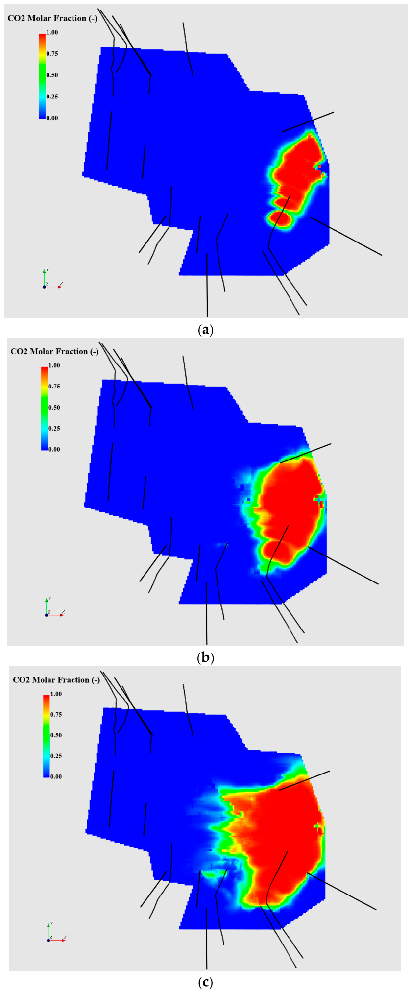
The simulated CO2 mole-fraction distributions after 2, 5, and 10 years of injection are shown in Figure 14. The CO2-enriched region expands from the injector with time and develops an irregular spatial distribution, consistent with heterogeneous reservoir connectivity and the modeled fracture system. These maps identify the preferential migration pathways represented by the simulation and complement the production comparison in Figure 13. The presence of CO2 alone does not establish the amount of methane displaced, the timing of breakthrough at individual producers, or long-term storage security. Applying the regional inventory algorithm to the same polygon after injection gives a remaining gas volume of 2.39 × 10⁸ m3. Relative to the pre-injection inventory of 2.81 × 10⁸ m3, this represents a decrease of 4.2 × 10⁷ m3, or 14.9%; approximately 48.7% of the initial regional inventory remains. The inventory calculation must retain the same hydrocarbon-component definition and exclude injected CO2.
4. Conclusions
An integrated workflow combining boundary element fracture modeling, EDFM-AI history matching, and automated polygon-based gas accounting was applied to a 14-well Sulige tight gas reservoir. The workflow links stimulation-derived fracture geometry to production-constrained flow behavior and regional resource assessment. The principal findings are as follows.
The best-matching model yields effective-to-wetted fracture half-length ratios of 57–75% and height ratios of 54–70%, with a fracture conductivity of approximately 10 mD·m. These results distinguish the stimulation-contacted extent from the equivalent conductive geometry required to reproduce the pressure history under prescribed gas-production rates. The calibrated dimensions are model-dependent effective parameters rather than a unique reconstruction of the subsurface fracture system.
Automated polygon-based accounting quantifies the remaining gas within an irregular candidate injection area containing two horizontal wells and three vertical wells. After 20 years of depletion, its gas inventory decreases from 4.91 × 10⁸ to 2.81 × 10⁸ m3, leaving 57.2% of the initial regional volume. This in-place inventory supports further evaluation of injection opportunities but does not directly quantify recoverable reserves.
For the evaluated 10-year CO2-injection scenario at 35 MPa, cumulative methane production at year 30 increases from 2.31 × 10⁸ to 2.52 × 10⁸ m3 relative to continued depletion. The incremental production of 2.1 × 10⁷ m3 represents a 9.1% relative increase, while the reported recovery factor rises from 47.0% to 51.3%, a gain of 4.3 percentage points. The simulated CO2 distributions show progressive, heterogeneous migration away from the injector.
The post-injection regional gas inventory is 2.39 × 10⁸ m3, a decrease of 14.9% from the pre-injection value. This net regional change reflects production and redistribution across the polygon boundary and must be distinguished from incremental methane recovery relative to the no-injection case. Together, the inventory analysis and production comparison provide complementary measures for screening injection targets and evaluating CO2-EGR scenarios. The predicted benefit remains conditional on the calibrated model and operating assumptions; forecast uncertainty, well-specific CO2 breakthrough, and alternative injection strategies require further assessment before operational implementation.
Author Contributions
Conceptualization, L.L., Y.Y.; methodology, P.L., W.L..; investigation, Y.S., C.W.; writing—original draft preparation, M.Y.; writing—review and editing, P.C., C.L., W.Y. All authors have read and agreed to the published version of the manuscript.”.
Funding
1. Research on Energy Replenishment Technology for Enhanced Gas Recovery in Tight Gas Reservoirs (2023ZZ25YJ05); 2. Research on Well Pattern Density Optimization for Enhancing Recovery Rate Technology (2025ZD1405503).
Data Availability Statement
Data are unavailable due to privacy or ethical restrictions.
Conflicts of Interest
The authors declare no conflicts of interest.
Abbreviations
The following abbreviations are used in this manuscript:
| CO2-EGR | CO2-enhanced gas recovery |
| EDFM | Embedded discrete fracture model |
References
- Oldenburg, C.M.; Pruess, K.; Benson, S.M. Process modeling of CO2 injection into natural gas reservoirs for carbon sequestration and enhanced gas recovery. Energy Fuels 2001, 15(2), 293–298. [Google Scholar] [CrossRef]
- Hughes, T.J.; Honari, A.; Graham, B.F.; Chauhan, A.S.; Johns, M.L.; May, E.F. CO2 sequestration for enhanced gas recovery: New measurements of supercritical CO2–CH4 dispersion in porous media and a review of recent research. Int. J. Greenh. Gas. Control 2012, 9, 457–468. [Google Scholar] [CrossRef]
- Patel, M.J.; May, E.F.; Johns, M.L. High-fidelity reservoir simulations of enhanced gas recovery with supercritical CO2. Energy 2016, 111, 548–559. [Google Scholar] [CrossRef]
- Jia, Y.; Shi, Y.; Pan, W.; Huang, L.; Yan, J.; Zhao, Q. The feasibility appraisal for CO2 enhanced gas recovery of tight gas reservoir: Experimental investigation and numerical model. Energies 2019, 12(11), 2225. [Google Scholar] [CrossRef]
- Ding, J.; Yan, C.; He, Y.; Wang, C. Supercritical CO2 sequestration and enhanced gas recovery in tight gas reservoirs: Feasibility and factors that influence efficiency. Int. J. Greenh. Gas. Control 2021, 105, 103234. [Google Scholar] [CrossRef]
- Ding, J.; Yan, C.; Wang, G.; He, Y.; Zhao, R. Competitive adsorption between CO2 and CH4 in tight sandstone and its influence on CO2-injection enhanced gas recovery (EGR). Int. J. Greenh. Gas. Control 2022, 113, 103530. [Google Scholar] [CrossRef]
- Liao, H.; Pan, W.; He, Y.; Fang, X.; Zhang, Y. Study on the mechanism of CO2 injection to improve tight sandstone gas recovery. Energy Rep. 2023, 9, 645–656. [Google Scholar] [CrossRef]
- Zhao, E.; Jin, Z.; Li, G.; Zhang, K.; Zeng, Y. Numerical simulation of CO2 storage with enhanced gas recovery in depleted tight sandstone gas reservoirs. Fuel 2024, 371, 131948. [Google Scholar] [CrossRef]
- Zhao, E.-M.; Jin, Z.-J.; Li, G.-S.; Zhang, K.-Q.; Zeng, Y. Feasibility of CO2 storage and enhanced gas recovery in depleted tight sandstone gas reservoirs within multi-stage fracturing horizontal wells. Pet. Sci. 2024, 21(6), 4189–4203. [Google Scholar] [CrossRef]
- Hu, J.; Yang, S.; Yang, K.; Deng, H.; Wang, M.; Li, J.; Gao, X. Enhanced gas recovery coupled with CO2 sequestration in tight sandstone reservoirs with different pore-throat structures. Energy Fuels 2024, 38(13), 12005–12023. [Google Scholar] [CrossRef]
- Hu, J., Yang, S., Zhang, Y., Jiang, H., Shen, B., He, Y., Zhao, S., Gao, X., and Deng, H. 2026. Reservoir-scale numerical simulation of enhanced gas recovery coupled with CO2 multi-storage mechanisms in water-bearing tight sandstone gas reservoir. Geoenergy Science and Engineering. Advance online publication, article 214664. [CrossRef]
- Wang, J.; Elsworth, D. Role of proppant distribution on the evolution of hydraulic fracture conductivity. J. Pet. Sci. Eng. 2018, 166, 249–262. [Google Scholar] [CrossRef]
- Dong, C.Y.; de Pater, C.J. Numerical implementation of displacement discontinuity method and its application in hydraulic fracturing. Comput. Methods Appl. Mech. Eng. 2001, 191(8-10), 745–760. [Google Scholar] [CrossRef]
- Moinfar, A.; Varavei, A.; Sepehrnoori, K.; Johns, R.T. Development of an efficient embedded discrete fracture model for 3D compositional reservoir simulation in fractured reservoirs. SPE J. 2014, 19(2), 289–303. [Google Scholar] [CrossRef]
- Tripoppoom, S.; Xie, J.; Yong, R.; Wu, J.; Yu, W.; Sepehrnoori, K.; Miao, J.; Chang, C.; Li, N. Investigation of different production performances in shale gas wells using assisted history matching: Hydraulic fractures and reservoir characterization from production data. Fuel 2020, 267, 117097. [Google Scholar] [CrossRef]
- Wu, K.; Olson, J.E. A simplified three-dimensional displacement discontinuity method for multiple fracture simulations. Int. J. Fract. 2015, 193, 191–204. [Google Scholar] [CrossRef]
- Wu, K.; Olson, J.E. Numerical investigation of complex hydraulic-fracture development in naturally fractured reservoirs. SPE Prod. Oper. 2016, 31(4), 300–309. [Google Scholar] [CrossRef]
- Liu, S., Valkó, P.P. 2015. An improved equilibrium-height model for predicting hydraulic fracture height migration in multi-layer formations. Paper SPE 173335, SPE Hydraulic Fracturing Technology Conference, The Woodlands, Texas, USA, 3-5 February.
- Xu, Y.; Cavalcante Filho, J.S.A.; Sepehrnoori, K.; Yu, W. Discrete-fracture modeling of complex hydraulic-fracture geometries in reservoir simulators. SPE Reserv. Eval. Eng. 2017, 20, 403–422. [Google Scholar] [CrossRef]
- Xu, Y.; Yu, W.; Sepehrnoori, K. Modeling dynamic behaviors of complex fractures in conventional reservoir simulators. SPE Reserv. Eval. Eng. 2019, 22, 1110–1130. [Google Scholar] [CrossRef]
- Liu, C., Xie, H., Mao, Z., Yu, W., Li, N., Gong, Y., Leines, J., Miao, J., Sepehrnoori, K. 2023. EDFM-AI for calibration of hydraulic and natural fracture geometry. Paper ARMA 23–0083, the 57th US Rock Mechanics/Geomechanics Symposium, Atlanta, Georgia, USA, 25-28 June.
Figure 1.
Three-dimensional geomechanical property distributions used for hydraulic-fracture modeling: (a) Young’s modulus; (b) Poisson’s ratio; (c) minimum horizontal stress; and (d) maximum horizontal stress.
Figure 1.
Three-dimensional geomechanical property distributions used for hydraulic-fracture modeling: (a) Young’s modulus; (b) Poisson’s ratio; (c) minimum horizontal stress; and (d) maximum horizontal stress.
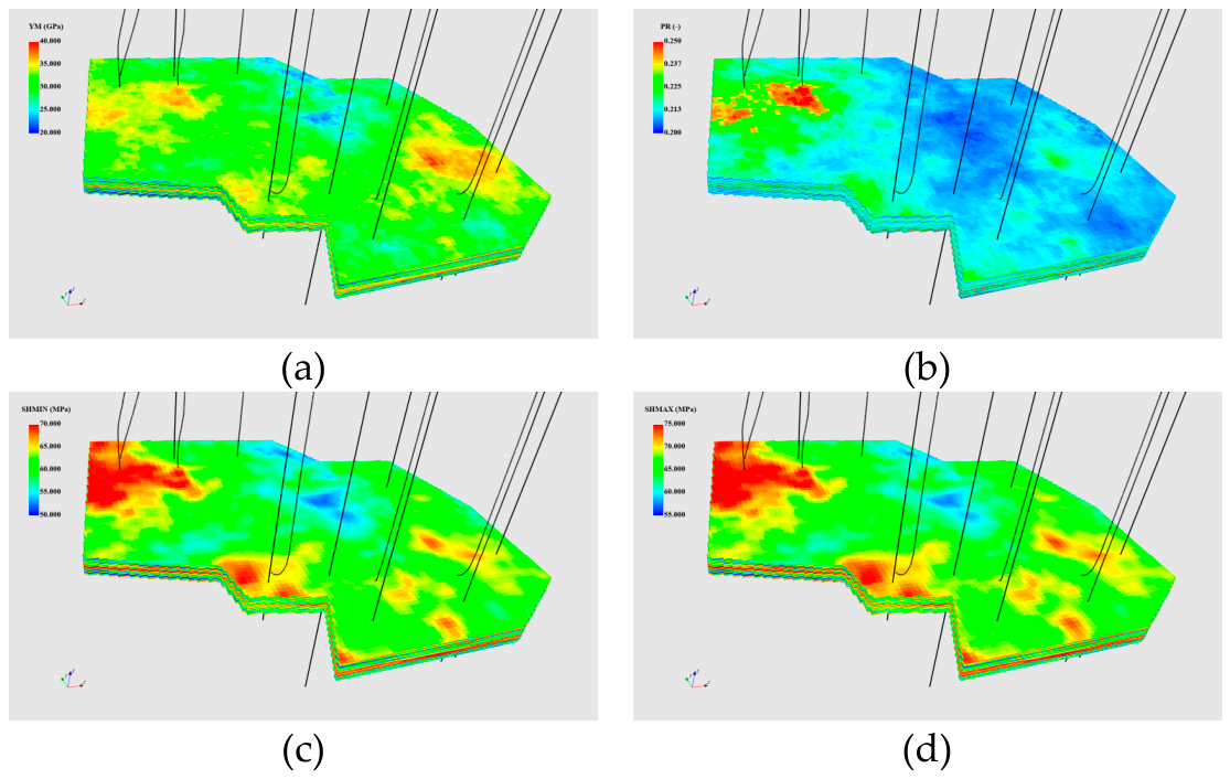
Figure 2.
Simulated hydraulically wetted fracture geometry for the 14-well study area.
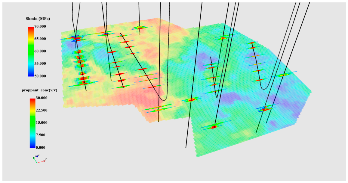
Figure 3.
Simulated wetted fracture geometry for representative wells: (a) horizontal well; and (b) vertical well.
Figure 3.
Simulated wetted fracture geometry for representative wells: (a) horizontal well; and (b) vertical well.
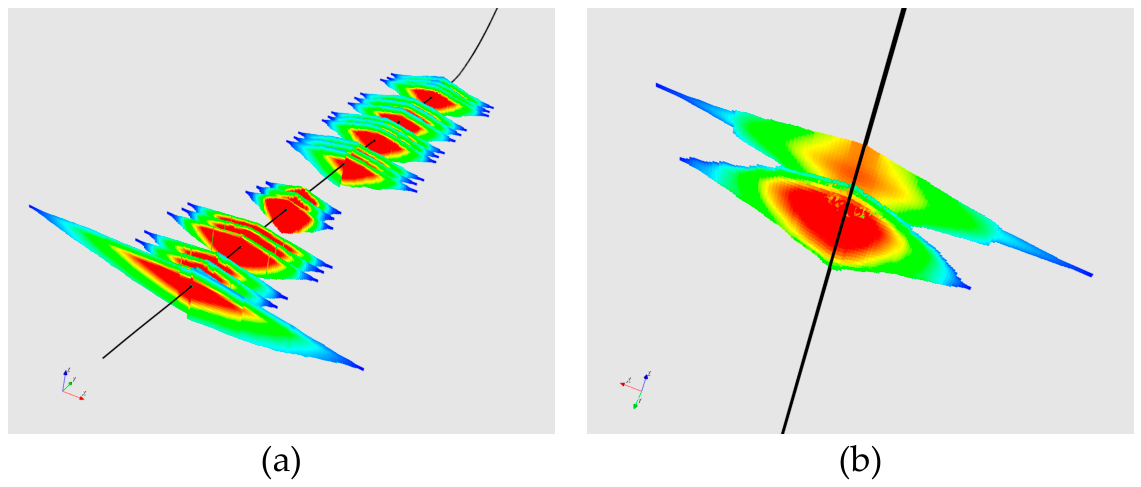
Figure 4.
Three-dimensional reservoir property distributions: (a) porosity; (b) permeability; (c) initial water saturation; and (d) initial reservoir pressure.
Figure 4.
Three-dimensional reservoir property distributions: (a) porosity; (b) permeability; (c) initial water saturation; and (d) initial reservoir pressure.
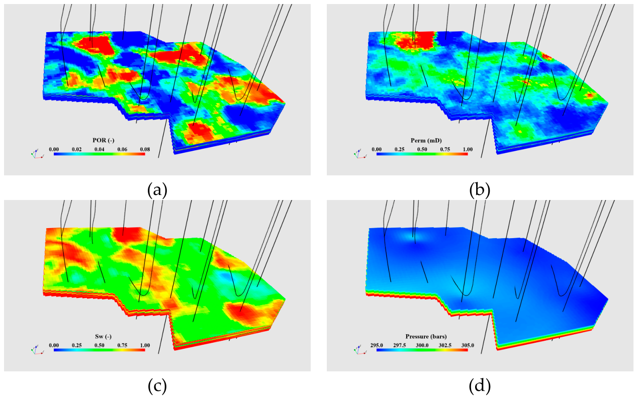
Figure 5.
Gas–water relative-permeability curves for (a) the matrix and (b) hydraulic fractures. The horizontal and vertical axes denote gas saturation and relative permeability, respectively; the red and blue curves represent gas and water.
Figure 5.
Gas–water relative-permeability curves for (a) the matrix and (b) hydraulic fractures. The horizontal and vertical axes denote gas saturation and relative permeability, respectively; the red and blue curves represent gas and water.
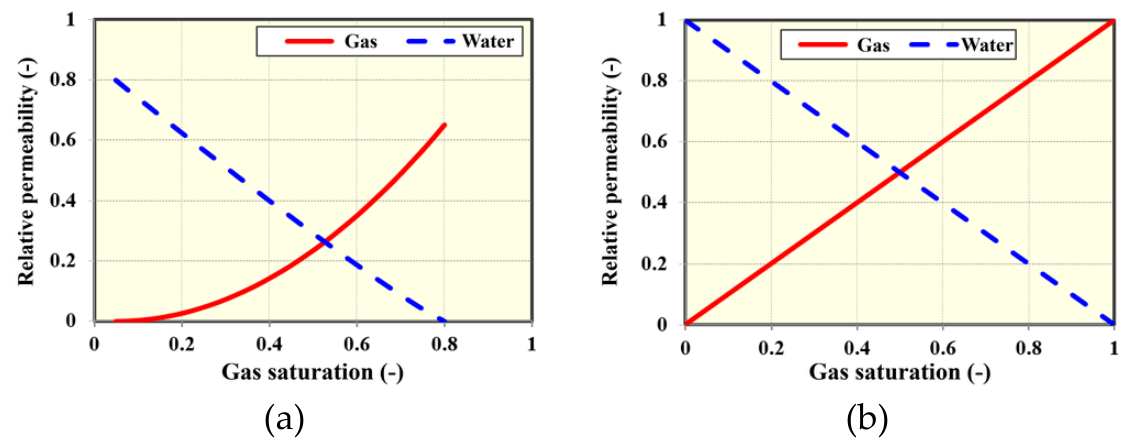
Figure 6.
Representative horizontal-well data and simulation responses used in automated history matching: (a) prescribed gas-production rate; and (b) bottomhole pressure. The pressure comparison includes the retained realizations and best-matching response.
Figure 6.
Representative horizontal-well data and simulation responses used in automated history matching: (a) prescribed gas-production rate; and (b) bottomhole pressure. The pressure comparison includes the retained realizations and best-matching response.
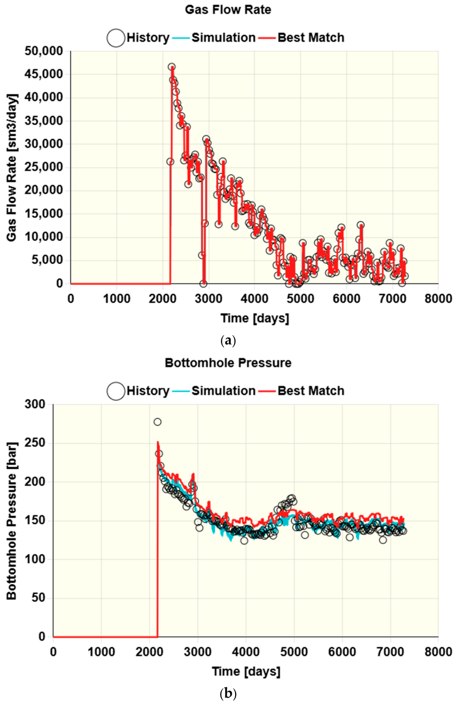
Figure 7.
Representative vertical-well data and simulation responses used in automated history matching: (a) prescribed gas-production rate; and (b) bottomhole pressure. The pressure comparison includes the retained realizations and best-matching response.
Figure 7.
Representative vertical-well data and simulation responses used in automated history matching: (a) prescribed gas-production rate; and (b) bottomhole pressure. The pressure comparison includes the retained realizations and best-matching response.
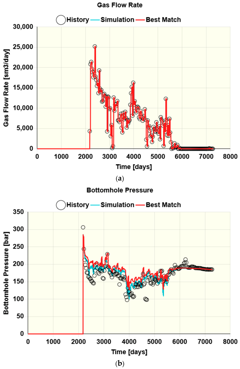
Figure 8.
Production-effective hydraulic-fracture geometry for the 14 wells in the best-matching reservoir realization.
Figure 8.
Production-effective hydraulic-fracture geometry for the 14 wells in the best-matching reservoir realization.
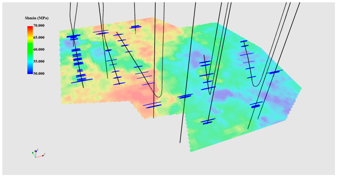
Figure 9.
Simulated reservoir-pressure distributions after (a) 10 years and (b) 20 years of depletion production.
Figure 9.
Simulated reservoir-pressure distributions after (a) 10 years and (b) 20 years of depletion production.
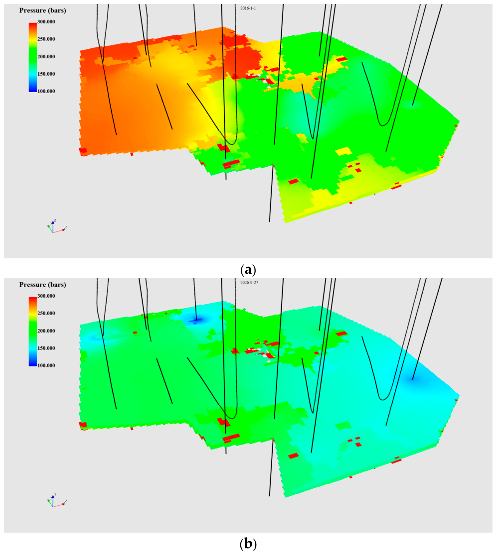
Figure 10.
Simulated gas-saturation distributions after (a) 10 years and (b) 20 years of depletion production.
Figure 10.
Simulated gas-saturation distributions after (a) 10 years and (b) 20 years of depletion production.
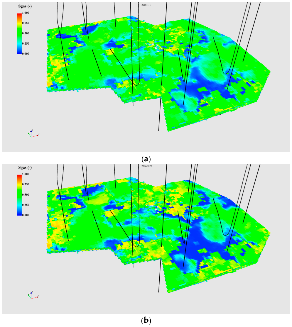
Figure 11.
Polygon-defined candidate injection area used for automated regional remaining-gas inventory calculation. The selected area contains two horizontal wells and three vertical wells.
Figure 11.
Polygon-defined candidate injection area used for automated regional remaining-gas inventory calculation. The selected area contains two horizontal wells and three vertical wells.
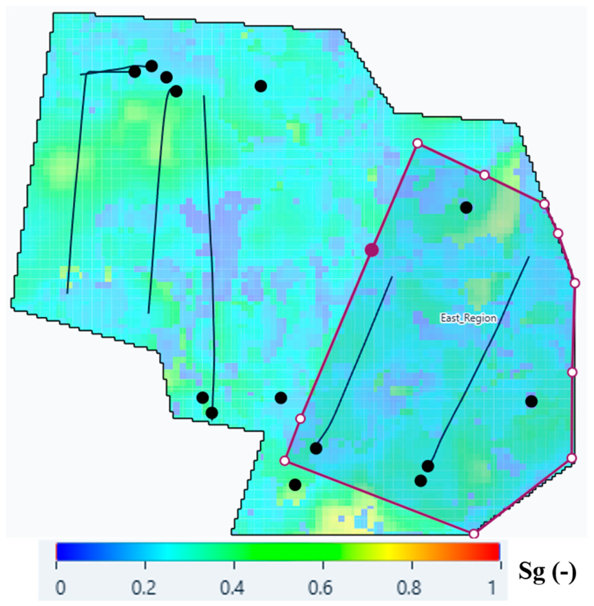
Figure 12.
Simulated CO2-injection rate and cumulative injected volume under a 35 MPa injection-pressure constraint.
Figure 12.
Simulated CO2-injection rate and cumulative injected volume under a 35 MPa injection-pressure constraint.
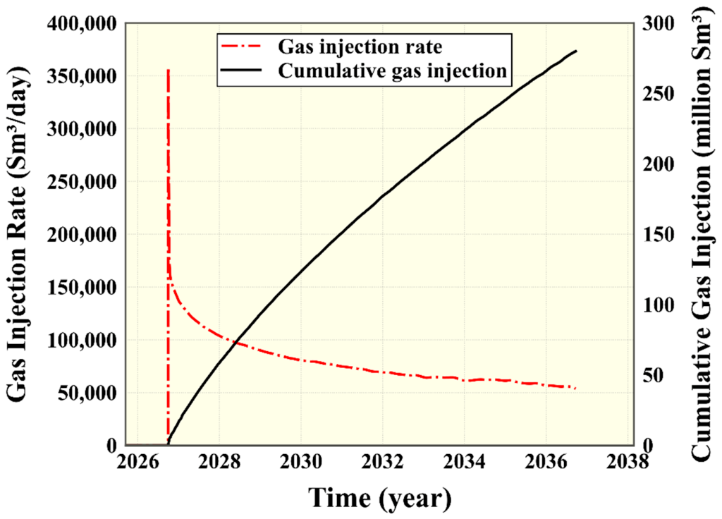
Figure 13.
Forecast comparison with and without CO2 injection: (a) cumulative methane production; and (b) the reported methane recovery factor.
Figure 13.
Forecast comparison with and without CO2 injection: (a) cumulative methane production; and (b) the reported methane recovery factor.
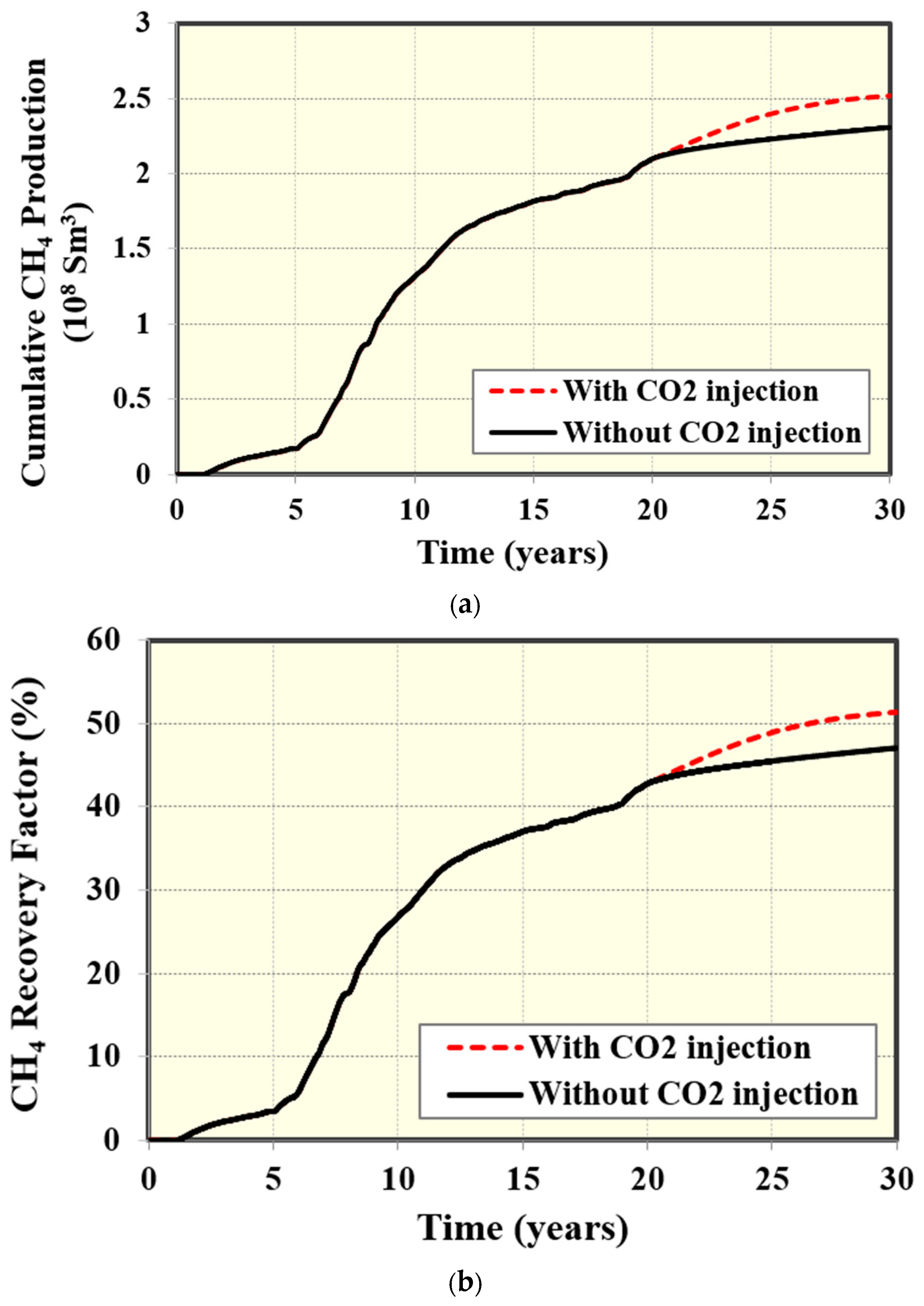
Figure 14.
Simulated CO2 mole-fraction distributions after (a) 2 years, (b) 5 years, and (c) 10 years of injection.
Figure 14.
Simulated CO2 mole-fraction distributions after (a) 2 years, (b) 5 years, and (c) 10 years of injection.
Disclaimer/Publisher’s Note: The statements, opinions and data contained in all publications are solely those of the individual author(s) and contributor(s) and not of MDPI and/or the editor(s). MDPI and/or the editor(s) disclaim responsibility for any injury to people or property resulting from any ideas, methods, instructions or products referred to in the content. |
© 2026 by the authors. Licensee MDPI, Basel, Switzerland. This article is an open access article distributed under the terms and conditions of the Creative Commons Attribution (CC BY) license (http://creativecommons.org/licenses/by/4.0/).
Copyright: This open access article is published under a Creative Commons CC BY 4.0 license, which permit the free download, distribution, and reuse, provided that the author and preprint are cited in any reuse.