

Submitted:
30 October 2026
Posted:
03 November 2026
You are already at the latest version
Abstract
A prolate spheroidal model of axisymmetric hollow ellipsoid is usually used for the analytical estimation of magnetic signature of ships and vessels. To overcome several limitations of the model such as the rotational symmetry, a general solution of the problem for a triaxial ellipsoid without the rotational symmetry is presented. The true analytical solution is derived in terms of elliptic integrals of the first and second kind. The presented solution is validated by the comparison with the results from a finite element analysis. The ellipsoidal system of coordinates implies that the outer and inner surfaces of a hollow ellipsoid are confocal. This leads to the analytical model of vessel hull with a variable wall thickness. The thickness variation depends on the hull aspect ratio, and it may lead to an inaccurate estimation of the magnetic signature. To overcome this limitation, the hollow ellipsoidal body with the non-confocal outer and inner surfaces is also considered, so that the thickness of the vessel hull is the same in all directions. The magnetic signature in this case can be significantly different from the case of the hollow ellipsoid with the confocal surfaces. In addition to the magnetic field outside the ellipsoid, the field inside the wall and in the cavity is analyzed. As a result of this analysis the formulas for the shielding effectiveness and magnetic moment are derived and validated. Also, cases of an axial symmetry when the triaxial ellipsoid transforms into the sphere, prolate or oblate spheroids are considered.
Keywords:
magnetic signature
; hollow triaxial ellipsoid
; magnetic moment
; shielding effectiveness
1. Introduction
This paper presents a general solution of magnetostatic problem of a hollow triaxial ellipsoid in the uniform applied field. In case of rotational symmetry over one of ellipsoid axes there is a complete analytical solution of the problem presented in the public domain [1,2]. Both solutions are derived in spheroidal coordinates for the prediction of ship’s magnetic signature and hull magnetization in the Earth’s field. However, these models have few major limitations. First, the wall thickness in the model is variable, and it depends on the ellipsoid aspect ratio. The ratio of maximum to minimum thickness is approximately proportional to the axis ratio of the prolate ellipsoid. The length of hull is usually few times larger than its width. Therefore, if we approximate the hull by the prolate spheroid of equivalent size the wall thickness along the hull appears to be few times smaller than along its width. Apparently, this may cause a significant error in the prediction of hull magnetization. To lift this inherent limitation of ellipsoidal system of coordinates, we propose a new analytic solution for the prolate spheroidal ellipsoid with the equal wall thickness.
A second major limitation of the known analytical solution is the axisymmetry that requires the equal sizes of the hull in the direction transverse to the applied field. The axisymmetric model also implies that the field is applied along the model symmetry axis, and this also reduces the application range of the axisymmetric model. To overcome this restriction, we present a new general solution of magnetostatic problem of a triaxial hollow ellipsoid in the uniform applied field oriented arbitrary. Usually, analytical solutions for the axisymmetric case are derived in the prolate spheroidal system of coordinates. However, if the ellipsoidal body is solid a well-known solution is given for example by Landau and Lifshitz [3] in a general ellipsoidal coordinate system. Indeed, the interface conditions for the magnetic scalar potential and its derivative are applied on the ellipsoidal coordinate surfaces regardless of two other coordinates. We extend this approach for deriving the analytical solution when the triaxial ellipsoid is hollow.
In this work, we focus on the magnetostatic solution with the application to a magnetic signature of the magnetized hollow ellipsoidal body. However, the shielding efficiency and magnetic moment of the ellipsoidal shell are also considered. The approximation of the hull using its magnetic moment is quite useful for the prediction of magnetic signatures far from the ship. The results presented can be extended to other applications related to magnetic objects or particles of ellipsoidal shape with cavities. Also, the solution easily can be applied to the electrostatic field if the magnetic permeability of ellipsoid is replaced by the electric permittivity.
The paper is structured as follows. First, the axisymmetric ellipsoidal (or prolate spheroidal) shell with the equal wall thickness in the uniform external magnetic field is considered. The solution is presented in the series of Legendre functions. Then, a general solution of magnetic field problem for the hollow triaxial ellipsoid with the confocal inner and outer surfaces is given in terms of elliptic integrals. Next, the analytical solution of the hollow confocal ellipsoid is applied to the triaxial shell with the equal wall thickness. Finally, the formulas for magnetic shielding, demagnetization, and magnetic moment of hollow triaxial ellipsoid are derived.
2. Hollow Ellipsoid with Non-Confocal Outer and Inner Surfaces
Let’s consider the ellipsoidal shell with the equal wall thickness, t placed in the uniform external field applied along z-direction. The magnetic permeability of the shell is constant, and the surrounding air has the permeability of free space. For the sake of simplicity, let’s consider the axisymmetric case first. We introduce the prolate spheroidal coordinates in accordance with Smythe [4]:
where a and c are semi-axes along the radial and axial direction, respectively, ξ and η are the ellipsoidal surfaces and hyperboloids of one sheet, respectively. The relation between the polar and ellipsoidal coordinates of the first coordinate system is
Where
Unlike a traditional way of modeling the prolate spheroid [1] we have to use now two ellipsoidal coordinate system (ξ,η) and (ξ′,η′). Indeed, the wall thickness of the hollow ellipsoid with the outer and inner surfaces coinciding with the coordinate surfaces ξ = ξ1 and ξ= ξ2 is variable (Figure 1).
The relation between the wall thickness along z- and r- axes is
or approximately tz ≈ tr a/c when a and c >> t. In order to have the same wall thickness, we introduce the second coordinate system with the same center but different aspect ratio for the axes. The axes of the second coordinate system are a1 = a − t and c1 = c − t. The hollow ellipsoidal body is between two non-confocal ellipsoidal surfaces defined in two systems of coordinates. The outer surface with the axes (a,c) coincides with the ellipsoidal surface ξ = ξ1 of the first system while the inner surface with axes (a1=a-t,c1=c-t) is defined as ξ′ = ξ′2 in the second system.
The scalar magnetic potential satisfies the Laplace equation
The solution of (5) in the area outside the hollow body l ξ > ξ1 can be presented by a series of Legendre functions of the first and second kind
Because of model symmetry only odd harmonics are kept in the series. The solution in the cavity 1 ≤ ξ′ ≤ ξ′2 is
Inside the wall ξ1 > ξ, ξ′ > ξ′2, we can express the solution either in the coordinates of the first system or using the second one:
The outer surface ξ = ξ1 can be presented by the sets of coordinates ξ′1〈ξ1,η〉 and η′1 〈ξ1,η〉 in the second coordinate system, and the inner surface ξ′ = ξ′2 is defined by the sets of coordinates ξ2〈ξ‘2,η‘〉 and η2 〈ξ‘2,η‘〉 in the first coordinate system. These sets can be determined from the relation between the coordinates of two systems:
where
These relations can be derived from (1)-(2) after expressing ρ and z consequently in coordinates (ξ,η) and (ξ′,η′ ) and then equalizing the expressions.
To map ξ = ξ1 in the second system, the coordinate η is subdivided in the interval [0,1] in N+1 points ηi =(i-1)/N, i=1,N+1 . Then the sets of coordinates ξ′1〈ξ1,ηi〉 and η′1〈ξ1,ηi〉 are calculated from (9) –(10) after substitution of ξ and η by ξ1 and ηi, respectively. The same routine is used also to find the sets of coordinates ξ2〈ξ‘2,η‘i〉 and η2 〈ξ‘2,η‘i〉 for ξ′ = ξ′2 in the first coordinate system.
The equations for the coefficients in series (6) ,(8) are found from the interface conditions for the potential and its derivative over ξ at ξ = ξ1
After substitution (6) and (8) in (11) and (12) , respectively, and multiplication of the result by Pn(η) , the integration over η in the range [-1,1] yields
where P’n(ξ) and Q’n(ξ) are the derivatives of Legendre functions dPn/dξ and dQn/dξ, respectively, δkn is the Kronecker delta . A similar manipulation is applied to the interface conditions on the inner surface ξ′ = ξ′2
As a result we obtain the relations between the coefficients of the magnetic potential in the wall and cavity
We can find two other relations between the coefficients Bn , Cn , B’n , C’n from the dual definition of the potential (8) in the wall
where
After excluding An, Dn, Cn and C’n we can reduce the system (13),14),(17)–(20) to two sets of equations for coefficients Bn and B’n only. The dimension of the resultant linear system of equations is 2N where N is the number or accounted harmonics in series (6)-(8).
The field components of induced field outside the ellipsoid are calculated by differencing the potential after omitting the excitation field. The transverse component Hr
where
The longitudinal component Hz
where
The major difference of the presented analytical solution from the known one derived by Holmes [1] is the additional Legendre harmonics caused by a non-confocal boundary of the ellipsoid walls. These harmonics have to be calculated accurately, and the precision depends on the quality of integration (21)-(24). The analytical solution has been compared with the results from 2D finite element analysis (FEA) [5] (Figure 2). The numerical tests are performed for the ferromagnetic material with the relative permeability of μ = 80, different aspect ratios a/c, and wall thickness t. The adaptive integration is used to evaluate the integrals (21)-(24) with the targeted accuracy. The number of integration points then falls within the range of few thousands (from 2000 to 3000). The required number of harmonics varies in the range between 3 and 7 depending on the ellipsoid aspect ratio, and only odd harmonics exist in the series for the magnetic potential. The lower number of harmonics gives a satisfactory result at the smaller wall thickness and aspect ratios. As we can see from Figure 2 the values for the induced field outside the magnetic hull of vessel match very well for both solutions. The discrepancy between the plotted values is less than 1% at the field peaks.
The outlined method can be extended to the case without the axial symmetry. This would require considering the third coordinateϕ, that is the same as an azimuthal angle in the spherical system of coordinates. Then, the partial solutions of the Laplace equation (5) are the products of the associated Legendre functions of the first and second kind times the angular harmonics cos mϕ or sin mϕ [4]. In general, the solution of (5) is expressed in a double series of the Legendre and angular harmonics that significantly complicates the analytical solution for the ellipsoid with the equal wall thickness. In the next Sections we will show that this may not be required, and the general solution of a triaxial hollow ellipsoid with the confocal inner and outer surfaces can be used instead to estimate the magnetic signature of the ellipsoid with the equal wall thickness.
3. Triaxial Ellipsoid in Uniform Applied Field
When the boundaries of ellipsoid coincide with the coordinate surfaces of ellipsoidal coordinate system, a general closed-form solution is possible even without a rotational symmetry [3,6,7]. The relation between the Cartesian coordinates and confocal ellipsoidal coordinates is defined as follows [3]:
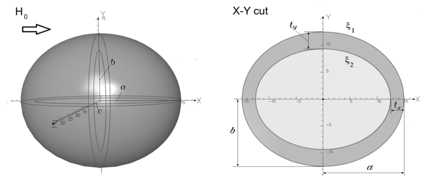
Figure 3.
Hollow triaxial ellipsoid in the uniform applied field.
Equation (27) is a cubic equation for u, and three roots are ξ, η, and ζ:
The constants ξ = const are ellipsoidal surfaces; η and ζ are hyperboloids of one and two sheets, respectively. Note, that the ellipsoidal coordinates ξ and η now are defined differently than in the previous section. The ellipsoidal coordinate plus square of semi axis ξ+a2 in this coordinate system corresponds to e2(ξ2-1) in the prolate spheroidal system of coordinates. The coordinate of hyperboloid surface η is equivalent to e2η2 in the prolate spheroidal system. We keep the notations for ellipsoidal coordinates the same. To distinguish between the systems, we add the range of definition for ellipsoidal coordinates. In this section we also use the conventional notations for the semi axes of a triaxial shell in the ellipsoidal system: a for x-axis, b for y-axis, and c for z-axis. However, in the following sections we alter this convention to have a > b> c.
The thickness of shell is variable. For example, the thickness in x-direction is the smallest root of a quadratic equation
where coordinate ξ2 = const defines the inner surface of ellipsoid. Two other values, ty , tz on axes y and z can be found from the similar equation with swapping axes a with b and c, respectively.
Assume the external field is applied in x-direction. If the field has other components the solution in general is a superposition of three similar parts of the same structure with the consequent swapping the Cartesian coordinates and semi axes. Let’s assume that the outer surface of the shell has three different semi axes: (a,b,c) , and the outer ellipsoidal surface coincides with the coordinate ξ1 = 0. The solution of (5) outside the shell ξ > ξ1 has a structure similar to this of a solid ellipsoid [3]:
where
In the shell wall ξ2 ≤ ξ ≤ ξ1
Inside the ellipsoidal cavity –c2 ≤ ξ < ξ2
Note, that integral Φ(ξ) can be expressed in terms of elliptic integrals [8] (Appendix I). The constants C1-C4 are determined from the continuity of the potential and its derivative times magnetic permeability on the inner (ξ2 < 0) and outer surfaces of the shell similar to (11)-(12),(15)-(16). The expressions for the constants are
When deriving formulas (34)-(38) the derivative Φ′(ξ) is replaced by the explicit values
Also, Rξ1 = abc and the potential on the outer boundary can be found as
where dx is the demagnetization factor along x-direction of a solid ellipsoid.
3.1. Magnetic Field Components
The component Hx of magnetic field in the direction of applied field and outside the shell is
The transverse component Hz
A similar formula can be written for Hy with replacing z by y.
The derivatives of coordinates can be found from (27) by differentiating the equation for ellipsoid by the Cartesian coordinate. For example
To find the explicit relation between Cartesian and elliptical coordinates, a cubic equation for ξ has to be solved (Appendix II)
3.2. Ellipsoidal Shell with Rotational Symmetry
The prolate and oblate spheroids can be considered now as partial cases of the triaxial ellipsoid with the rotational symmetry
3.2.1. Prolate Spheroid
In case of prolate spheroid, the equation of elliptical surface ξ is
where ρ and z are the radial and axial coordinates of cylindrical system, respectively, and a>b=c.
If the field is z-oriented the problem is axisymmetric, and we can swap x-coordinate with z in the formulas (29), (32)-(33) for the potential to keep them valid. Also, in this axisymmetric case, a is the semi axis in z-direction, and b = c is the semi axis of elliptical surface in the radial direction. The elliptical coordinate can be found from the quadratic equation
where
The elliptical coordinate is calculated from the cylindrical coordinates as
Apparently, there are only axial (or longitudinal) and radial (or transverse) field components of the induced field. The radial component of induced field is
where
The axial component of resultant field is
where
3.2.2. Oblate Spheroid
The oblate spheroid has the shortest semi axis along the axis of symmetry. Only if the field is –applied along this axis the field is axisymmetric. The equation of the ellipsoidal surface ξ is
where a=b>c. For this case, a is the semi axis in the radial direction, and b = c is the semi axis in the axial direction.
As we noticed, the analytical solution (29)-(33) for the potential can be adjusted for any arbitrary orientation of the applied field. When the field is applied in z-direction the coordinate x is replaced by z-coordinate in the expression for the potential. The function Φ(ξ) is modified as
Then, (34)–(37) for coefficients C1 – C4 are valid. The semi axes b and a should be replaced by a and c, respectively in (45)-(48). The solution for the potential in oblate spheroidal coordinates has the same structure as for the prolate spheroid given in Section 2. However, it is expressed in the products of Legendre functions of the real (for η) and imaginary (for ξ ) arguments [4].
3.3. Ellipsoidal Shell with About Equal Axes
When all three axes are of about the same value a ≈ b ≈ c, the elliptical shell apparently becomes a spherical one. The known solution for the dielectric spherical shell in the uniform applied field is given, for example, in the text book [3]. The solution for the magnetic spherical shell can be found by substitution of the dielectric permittivity by the magnetic permeability. Therefore, the field inside the spherical shell is
where a is the radius of the outer surface and t is the shell thickness.
To prove that solution (51) gives the same result when a=b=c, let’s consider the expression for the coefficient C4. For the three equal axes, the integral (30) can be expressed as follows
Note, that ξ2 =(a-t)2-a2, where t is the shell thickness. Also
After substitution of (52) and (53) in (38) we have
Also, now
After substitution C4 in (55) with the account of (54) we have
As we can conclude from (33) the field inside the cavity is equal to C2H0 that means it is the same as for the hollow sphere (51).
4. Validation of Solution for Hollow Triaxial Ellipsoid
The derived solution has been compared with the known one for the prolate spheroidal shell [1] as well as with the results from 2D finite element analysis [5] (Figure 4 and Figure 5). The numerical test is performed for the ferromagnetic material with the relative permeability of μ = 80, tz= 0.02, and different a/b ratios. The values for the induced field outside the magnetic hull of vessel [1] match very well for all three solutions. Note, that the field is applied along z-axis that is the axis of rotational symmetry.
For triaxial ellipsoids with different semi axes a ≠ b ≠ c, the results are presented in Figure 6 and Figure 7. The thickness of the shell in y- and z-axis is also different. For example, when a = 50, b = 10, c= 5 and for given tx= 0.02 m, the shell thicknesses in other directions are ty = 0.204 m and tz= 0.10 m.
Now, the field has no symmetry around x -axis aligned with the applied field. The solution (29)-(33) has been verified using 3D FEA [9]. The field is plotted along three lines parallel to x-axes equally distanced from it at 20 m. The peak of induced transverse field reaches the maximum on the line crossing y-axis. The magnetic signature has a minimum peak on the line crossing z-axis. Apparently, the peak value on the line parallel to x-axis crossing the point with coordinates y = z = 20/sqrt(2) m is in between of these two limits. For this case, the transverse field has two components Hz and Hy.
All presented results relate to the case when the applied field is oriented in x-axes, i.e., along the longest axes of shell. If the field is applied along other axis, say z, the function Φ(ξ) in the scalar potential is defined by (50). Apparently, the induced magnetic field in this case is weaker (Figure 8) than for the field applied along the longest axes (Figure 6 and Figure 7).
5. Ellipsoidal Shell with the Equal Thickness in All Directions
The analytical solution for the triaxial ellipsoid implies the shell thickness is different at least in the longitudinal and transvers directions. As we demonstrated earlier for the prolate spheroid, the equal wall thickness requires a different solution that can be presented in a series of the Legendre functions. For the triaxial hollow ellipsoid of equal wall thickness the solution is more complex, and requires a double series for harmonics. Therefore, it is of interest to consider whether the simple analytical solution for the hollow triaxial ellipsoid with the confocal surfaces can help in the estimation of magnetic signature when the thickness of elliptical shell is equal in all three directions.
Let’s consider first the prolate spheroidal shell (b = c) with the relative permeability of μ = 80. Figure 9 shows the comparison between the prediction of magnetic signature from the analytical solutions (45),(47) and (25)-(26) or FEA [5]. The non-confocal analytical and FEA models have the equal wall thickness along z- and ρ-axes, i.e., t = tz = tρ =0.02 m. The analytical solution (45),(47) is given for tρ = 0.02 m. However, the thickness in z-axes is different and depends on the axis ratio. If we neglect the quadratic term of thickness in (4) we can find that tz ≈ tρ b/a. Therefore, when a = 20 m and b = c= 10 m, tz = 0.01 m. The thickness tz is further reduced for the longer semi axis a.
Figure 9 shows that the analytical solution (45),(47) provides quite a good estimate of the magnetic signature for this selection in a wide range of a/b ratios. The relative discrepancy between the analytical solution and FEA at field peaks is less than 5% for the longitudinal component Bz and
4% for the transverse component Bρ . In contrast, if we select tz =0.02 m the analytical solution (45),(47) gives a significantly higher peaks (compare Figure 9 with Figure 4 and Figure 5). When the analytical solution is used with tz =0.02 m it may give a wrong impression that the magnetic signature is stronger for the longer hulls that is not the case if the thickness of ferromagnetic shell is held the same. The comparison for other values of wall thickness and distance from the hull is presented in Figure 10 and Figure 11. From this comparison we can conclude that the model with the confocal outer and inner ellipsoids can be used for shells with the equal wall thickness if the thickness in transverse direction tρ is equal to the actual thickness of shell, t. This conclusion is drawn for the axisymmetric shell. In case of triaxial shell the transverse thickness varies from ty to tz.. The question is what value to be used in the model of confocal ellipsoidal surfaces for the assessment of magnetic signature. The values of ty and tz can be calculated based on the equivalent amount of cross-sectional area of the wall. When equalizing the cross-sectional area of the hollow ellipsoid with the confocal boundaries and shell with the same wall thickness we have
Also, (28) yields
When tx << a, ty << b, tz << c , from (57)-(58) we can derive that the thicknesses of the equivalent confocal ellipsoid are
where t is the given wall thickness of the shell with the equally thick wall.
Figure 12 and Figure 13 present the comparison between the predictions from the analytical model (29)–(33) against the magnetic signature calculated by 3D FEA [9] for the ellipsoids of equal wall thickness. The comparison is performed along two lines parallel to x-axes, that is the direction of applied field. The magnetic signature peak on the line crossing y-axes is higher because it is closer to the ellipsoid as compared with the line crossing z-axes.
As we can see from the test results, the analytical model of confocal ellipsoids gives a good estimate of magnetic signature for the shell of equal wall thickness when the coordinate ξ2 of internal surface is selected in accordance with (59). The components of induced field are approximated with the maximum error of 5% at peaks. Therefore, in most practical cases when the wall thickness is significantly smaller than the ellipsoid axes, we may not need an additional correction of confocal model (29)-(33) similar to that considered in Section 2.
6. Shielding
So far we focused on the field outside the ellipsoid. However, there is another important application related to the magnetic field inside the cavity [10]. The field inside the ellipsoidal shield placed in the uniform field can be found from (33) as Hi = H0C2, i.e., it is a constant. Thus, the constant 1/C2 is a non-logarithmic effectiveness of the ellipsoidal shield: SE = H0 /Hi. After substitution (37) in (35) for C2 we have
To find the approximate expression for SE, let’s make few estimates. The difference of function Φ on two surfaces can be estimated as follows:
where ε is somewhere in the interval of [ξ2 , 0]. For a thin wall shell ε ≈ ξ2 /2. Alternatively, the integral (61) can be presented by any quadrature of a high accuracy. The determinant D in the expression of constant C2 can be estimated as
where dx is the demagnetization factor of the solid ellipsoid in x direction [3]:
After substitution (62) and (63) in (60) the shielding effectiveness is
For thin shells and high permeability materials, the formula for SE can be significantly simplified. If μ >> 1 and ξ2 ≈ -2atx ≈ -2bty ≈ -2ctz we can make the following approximations:
Then, SE can be approximated as
The indexes {x,y,z}and semi axes {a,b,c} are dependent on the field direction. Equation (67) is derived for the field applied along x–axis. If the field is applied in z-direction we swap the indexes and axes as follows
Similarly, swapping the indexes is required for the field applied in y-direction. For the prolate spheroidal shell, when the field is applied in x-direction and a > b= c, (67) can be simplified since ty= tz. It matches well with formula given by Mager [11] for prolate spheroidal shell with only one difference: the last term (tx/a) is ignored in [11] . From the approximate expression (67) we can see
That SE is proportional to the product of magnetic permeability and shell thickness. Thus, SE depends only on products μtu (u=x,y,z) and demagnetization factors du .
Figure 14 shows how SE for the ellipsoidal shell drops with increasing its aspect ratio. Also, from Figure 14 we can see that (67) approximates SE of thin wall shells even for relatively low values of magnetic permeability. Figure 15 illustrates the difference between the exact and approximate estimation of SE in case of ticker shells and lower magnetic permeability. The SE of a spherical shell
is given for the comparison. If the radius and thickness of spherical shell is equal to the average values of three semi axes and thicknesses, respectively, the SE of spherical shell is very close to the SE of ellipsoidal shell (Figure 14 and Figure 15). This is relevant of course for the ellipsoidal shells with the moderate values of aspect ratio. Figure 16 gives the SE for the same ellipsoidal shell in the transverse field applied along the shortest axis c. We can see that SE dependence on the aspect ratio is much weaker than for the longitudinal field. The SE limits for small and large aspect ratios are very close to SE of spherical and cylindrical shells [10], respectively calculated at the averaged wall thickness.
7. Demagnetization
Similar to a solid ellipsoid the demagnetizing field of hollow ellipsoid can be defined as a difference between the applied field and field defined by potential (32) inside the ellipsoid’s wall [3]. Unlike the solid ellipsoid, the demagnetizing field is a variable that can be defined from (32) as
Using the assessments (61)-(63), the constants C3 and C4 can be expressed explicitly. Thus, the demagnetizing field in the wall ξ2 ≤ ξ≤ 0 varies as follows:
The field reaches its maximum value on the internal surface ξ = ξ2 at x = a and minimum at x = 0. The field at these points can be calculated as:
where γ1 = 1 at ξ = ξ1 = 0 and γ1 = 0 at ξ =ξ2 ; γ2 = 1 at x = a and γ2 = 0 at x = 0.
For the thin wall and high permeability, Hdx can be assessed as
From (70) we can find that the demagnetizing field varies significantly over x (Figure 17) and a level of demagnetization of the ellipsoid’s wall is not the same. This differs from the case of a solid ellipsoid where the material is demagnetized uniformly. Figure 18 shows the demagnetizing field of ellipsoidal shell at x=0 in the longitudinal applied field for a various magnetic permeability and aspect ratios at the symmetry plane YZ.
8. Magnetization and Magnetic Moment
The magnetization of the ellipsoid and its magnetic moment can be found from the field inside the ellipsoid’s wall. The magnetization varies across the ellipsoid wall as
The magnetic moment of magnetized ellipsoid mx is the integral of magnetization over the ellipsoid’s volume. For the hollow ellipsoid, the integral of magnetization over the volume can be expressed using ∂ΨII/∂x on the outer and inner surfaces as follows:
where Vc is the volume of ellipsoid ‘s cavity
and V0 is the volume of solid ellipsoid
After substitution of coefficients C3 and C4 from (36) and (37) in (75), and accounting for (61),(63) we have
Note, that ε ≈ ξ2 /2 in (61) is true only for the relatively thin walls. For the thicker walls, the parameter ε shifts towards a larger negative value, so that it may reach ε ≈ 3ξ2 /4 when tz ≈ c.
For thin shells with a high permeability, (76) can be simplified
When tz → c, the hollow ellipsoid becomes a solid one. When the parameter Rξ2→ 0, the magnetic moment is equal to this of a solid ellipsoid [3]
When all three axes are of about the same value a ≈ b ≈ c, the consideration given above in Section 3.3 can be applied to demonstrate that (75) transforms into the expression for the magnetic moment of a hollow sphere of radius a thickness t
The magnetic moment of ellipsoid can be used, for example, when assessing the magnetic signature far enough from the magnetized body in a simple dipole approximation [12]:
where R is the distance between the center of dipole and observation point.
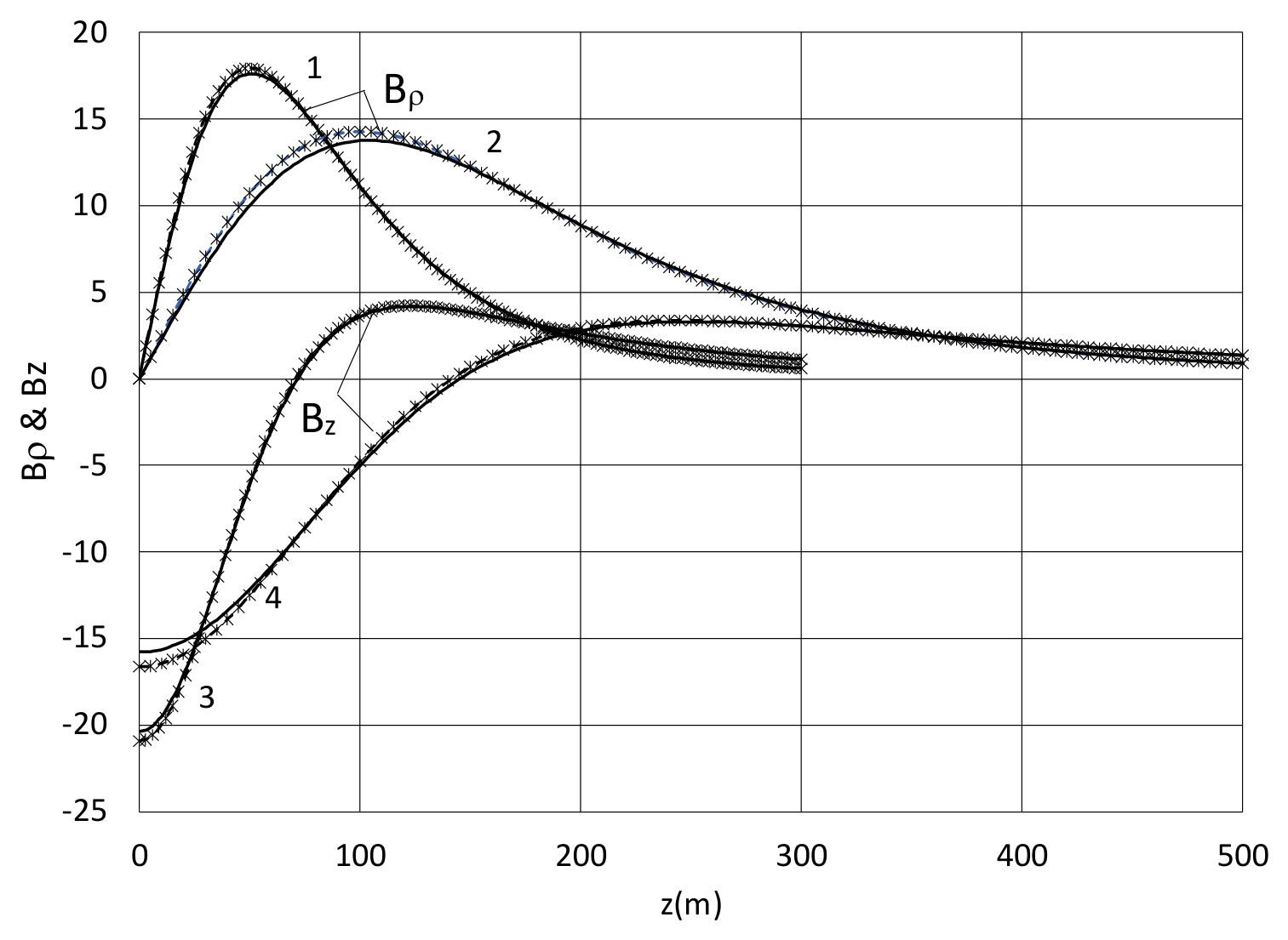
As expected, the dipole approximation (80) provides a good prediction of magnetic signature at distances far from the shell (Figure 19). For the shorter shell (a=20 m), it can be treated as a dipole at distances of order of 100 m. The relative deflection of the approximated field components Bρ and Bz from the exact peak values is less than 2% and 3%, respectively. For the longer shell (a=50m), the approximation (80) works at a larger distance. The approximation error for Bρ and Bz increases then to 3.5% and 5%, respectively.
9. Conclusions
A closed-form analytic solution for the magnetic potential of a hollow triaxial ellipsoid can be expressed in terms of elliptic integrals of the first and second kind. The solution has been validated by the comparison with FEA and previously published analytical solution for the magnetic signatures of axisymmetric vessel hulls.
The derived solution is perfectly suited for the assessment of the field outside and inside the magnetized elliptical shells and shields. The formulas for SE are derived for the cases of thick and thin walls. They agree well with the previously reported SE of the thin-walled prolate spheroids in the longitudinal field.
The solution for the triaxial ellipsoid is derived in the confocal ellipsoidal system of coordinates that imposes an unequal thickness of the ellipsoid’s wall. The predicted magnetic signature depends on the selection of the thickness taken as a reference for the distance between the outer and inner ellipsoidal surfaces. If we select the transverse thickness as a reference value the magnetic signature from the axisymmetric shell is very close to the one from a shell of the equal wall thickness.
For axisymmetric models, the solution derived earlier by Holmes [1] in prolate spheroidal coordinates is extended to the geometry with the non-confocal ellipsoidal surfaces. This allows us to predict the magnetic signature from ellipsoidal shells with the equal wall thickness. For the model with non-confocal ellipsoidal surfaces the solution is presented in the form of series of Legendre functions. This method can be extended to asymmetric models but requires a double series over the Legendre and angular harmonics. To avoid this in asymmetric models, we consider a simple method of finding the equivalent confocal ellipsoids to analyze the field of triaxial shell with the equal wall thickness. Then, the analytical solution for the triaxial ellipsoid can be used for the prediction of magnetic field outside the shell with the even wall thickness.
The accurate and approximate formulas are also derived for the magnetic moment of hollow ellipsoids. The asymptotic value of magnetic moment in case of a thick wall matches exactly to the moment of a solid ellipsoid. In addition, when all three axes are equal the magnetic moment of ellipsoid is the same as of a hollow sphere. The magnetic moment of shell can be used for the estimation of magnetic signature far from the magnetized body.
Appendix A
Scalar Potential Function
The scalar potential function can be expressed in terms of elliptic integrals as follows [8]:
where F and E are the incomplete elliptic integrals of the first and second kind, respectively.
Also.
If the external field is applied in a direction of shortest axis, c the expression for the potential is
For the external field applied in y-direction
In case of prolate spheroid a > b = c, when the field is applied along a (longest semi-axis):
In case of oblate spheroid, a = b> c, when the field is applied along c (shortest semi-axis):
Appendix B
Conversion from Cartesian to Ellipsoidal Coordinates
The expression for ellipsoidal coordinates at given Cartesian coordinates can be found as the roots of a cubic equation
where
References
- Holmes, J.J. Modeling a ship’s ferromagnetic signatures. In Syn. Lect. Comp. Electromag; 2007. [Google Scholar]
- Baker, F.E., Jr.; Brown, H. Magnetic induction of spherical and prolate spheroidal bodies with infinitesimally thin current bands having a common axis of symmetry and in a uniform inducing field, R&D report 20084; D. W. Taylor Naval Ship R&D Center: Bethesda, Maryland, 1982. [Google Scholar]
- Landau, L.D.; Lifshitz, E.M. Electrodynamics of continuous media; Pergamon Press: Oxford, 1960. [Google Scholar]
- Smythe, W.R. Static and Dynamic Electricity; Taylor and Francis, Bristol, PA, Pergamon Press: Oxford, 1989. [Google Scholar]
- Opera 2D, User Guide. Cobham Technical Services; Vector Fields Software: Kidlington, UK, Mar 2016.
- Morse, P.M.; Feshbach, H. Methods of theoretical physics; McGraw-Hill Book Company: New York, Toronto, London, 1953. [Google Scholar]
- Sihvola, A.H.; Lindell, I.V. Polarizability and effective permittivity of layered and continuously inhomogeneous dielectric ellipsoids. J. Electromagn. Waves Appl. 1990, vol.4(1), 1–26. [Google Scholar] [CrossRef]
- Gradshteyn, S.; Ryzhik, I. M. Table of integrals, Series, and Products., 2nd edition; Academic Press, 1980. [Google Scholar]
- Opera 3D, User Guide. Cobham Technical Services; Vector Fields Software: Kidlington, UK, Mar 2016.
- Kaden, H. Wirbelstrmeund Schirmung in der Nachrichtentechnick; Springer: Berlin, 1959. [Google Scholar]
- Mager, A. Magnetic shielding efficiencies of cylindrical shells with axis parallel to the field. J. Appl. Phys. 1968, vol.39, 1914. [Google Scholar] [CrossRef]
- Tamm, I.E. Fundamentals of the Theory of Electricity; Mir Publisher: Moscow, 1979. [Google Scholar]
- Abramowitz, M.; Stegun, I.A. Handbook of Mathematical Functions with Formulas, Graphs, and Mathematical Tables; Dover: New York, 1965. [Google Scholar]
Figure 1.
Ellipsoid with the equal wall thickness. The thickness t is the same along z- and ρ- axes. The outer surface coincides with the coordinate ξ = ξ1 of the first coordinate system while the inner surface aligns with the coordinate ξ’ = ξ’2 of the second system.
Figure 1.
Ellipsoid with the equal wall thickness. The thickness t is the same along z- and ρ- axes. The outer surface coincides with the coordinate ξ = ξ1 of the first coordinate system while the inner surface aligns with the coordinate ξ’ = ξ’2 of the second system.
Figure 2.
Longitudinal, Bz and transverse, Bρ (all positive) components of induced field from the ellipsoid of equal wall thickness and semi axis c = 10 m in the uniform field of 5.5E4 nTesla at r = 20 m: a = 20 m, t = 0.02 m (1); a = 20 m, t = 0.04 m (2) ; a = 50 m, t = 0.04 m (3). Solid line = analytical solution ; o = FEA.
Figure 2.
Longitudinal, Bz and transverse, Bρ (all positive) components of induced field from the ellipsoid of equal wall thickness and semi axis c = 10 m in the uniform field of 5.5E4 nTesla at r = 20 m: a = 20 m, t = 0.02 m (1); a = 20 m, t = 0.04 m (2) ; a = 50 m, t = 0.04 m (3). Solid line = analytical solution ; o = FEA.
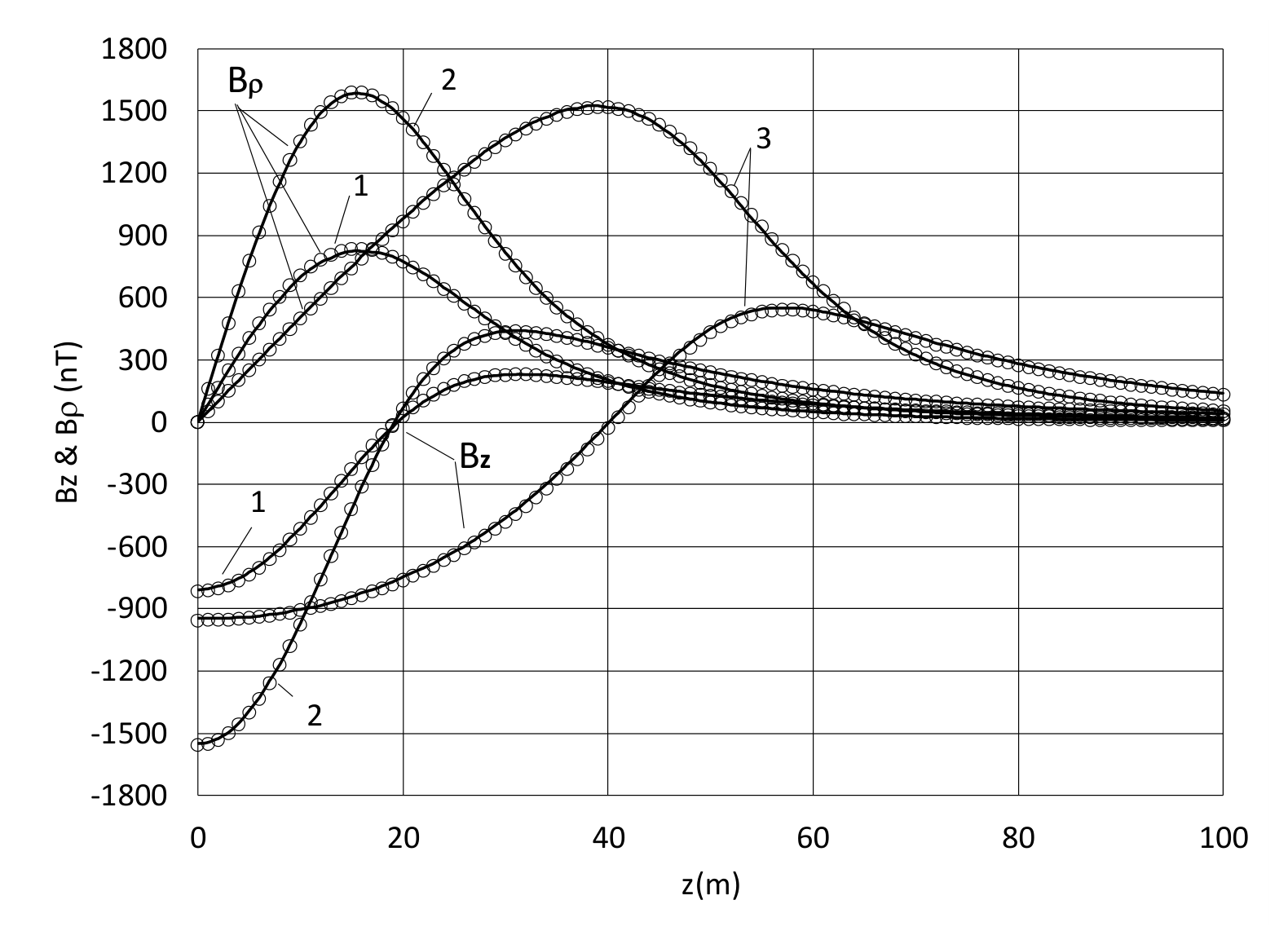
Figure 4.
Transverse component of induced field from an axisymmetric ellipsoidal shell in the uniform field of 5.5E4 nTesla at b = c = 10 m, tz= 0.02 m, ρ = 20 m: solid line = analytical solution (45), × = solution by Holmes [1], o–FEA [5]; a = 20 m (1); 50 m (2).
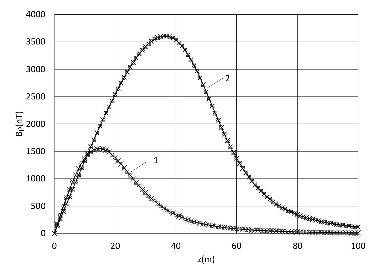
Figure 5.
Longitudinal component of induced field from the axisymmetric ellipsoidal shell in the uniform field of 5.5E4 nTesla at b = c =10 m, tz= 0.02 m, ρ = 20 m: solid line = analytical solution (47), × = solution by Holmes [1], o–FEA [5]; a = 20 m (1); 50 m (2).
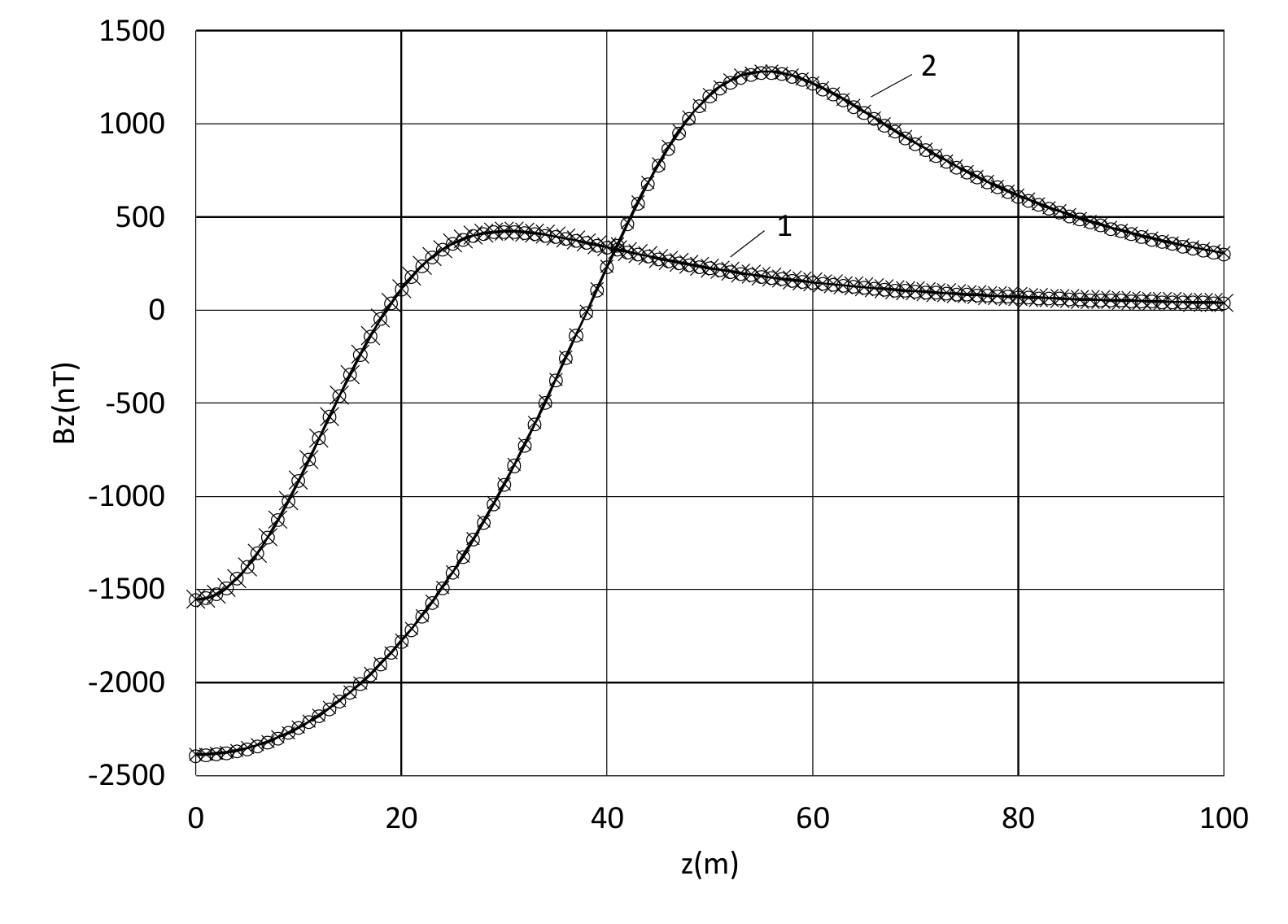
Figure 6.
Transverse components of induced field from the triaxial ellipsoidal shell of a = 50 m b = 10 m, c =5 m in the uniform field of 5.5E4 nTesla: By at y = 20 m & z=0 (1); sqrt (By^2+Bz^2) at y = z = 20/sqrt(2) m (2); Bz at y = 0 & z = 20 m (3): solid line = analytical solution (42), o–FEA [9].
Figure 6.
Transverse components of induced field from the triaxial ellipsoidal shell of a = 50 m b = 10 m, c =5 m in the uniform field of 5.5E4 nTesla: By at y = 20 m & z=0 (1); sqrt (By^2+Bz^2) at y = z = 20/sqrt(2) m (2); Bz at y = 0 & z = 20 m (3): solid line = analytical solution (42), o–FEA [9].
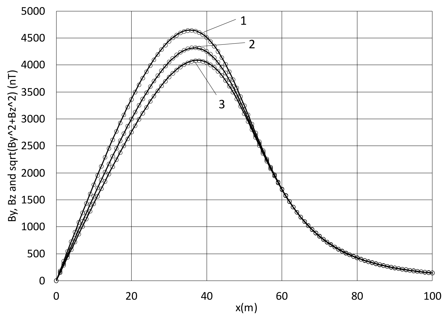
Figure 7.
Longitudinal component Bx of induced field from the triaxial ellipsoidal shell of a = 50 m, b = 10 m, c = 5 m in the uniform field of 5.5E4 nTesla at y = 20 m & z= 0 (1); at y = z = 20/sqrt(2) m (2); at y = 0 & z= 20 m (3): solid line = analytical solution (41), o–FEA [9].
Figure 7.
Longitudinal component Bx of induced field from the triaxial ellipsoidal shell of a = 50 m, b = 10 m, c = 5 m in the uniform field of 5.5E4 nTesla at y = 20 m & z= 0 (1); at y = z = 20/sqrt(2) m (2); at y = 0 & z= 20 m (3): solid line = analytical solution (41), o–FEA [9].
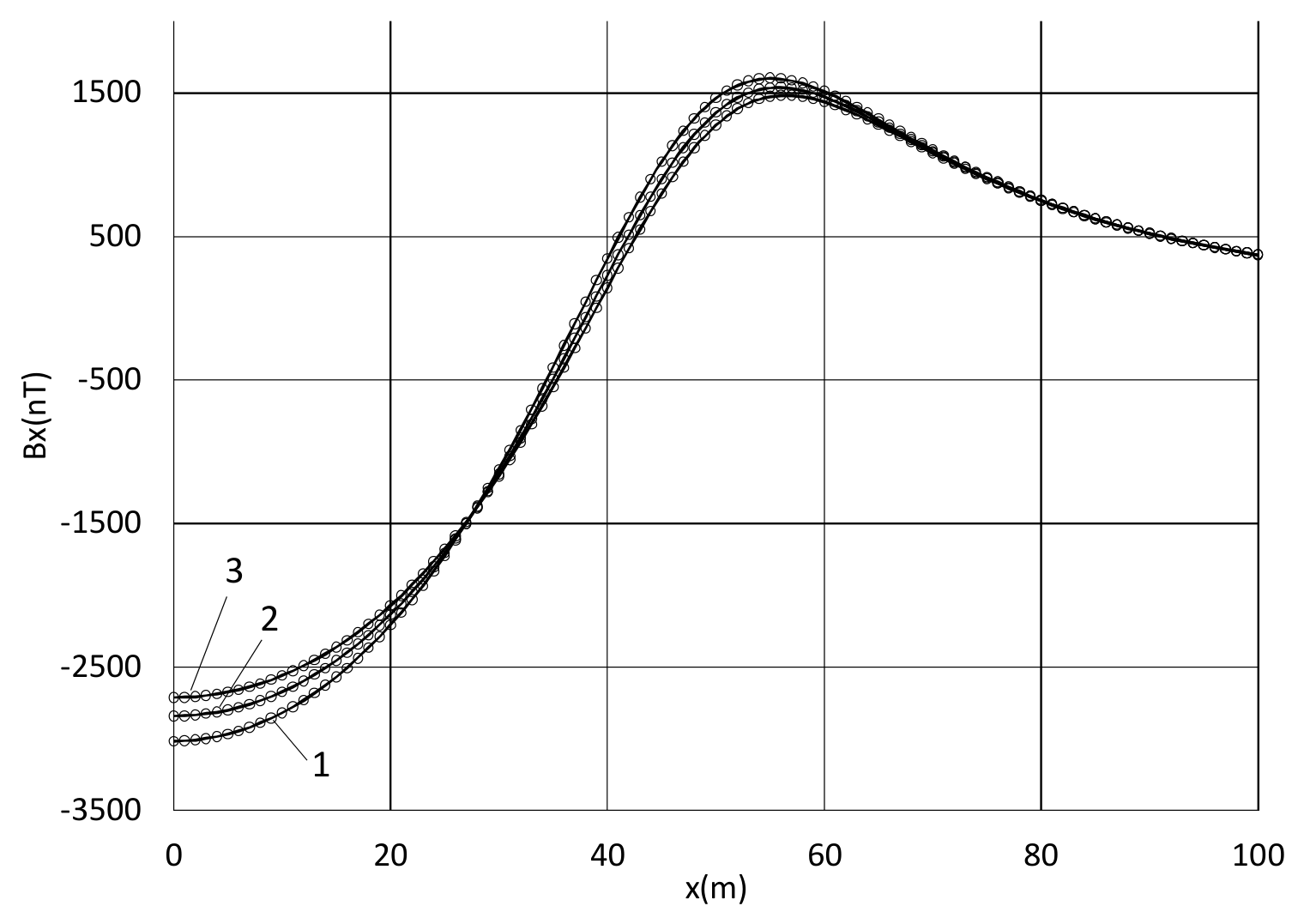
Figure 8.
Longitudinal (Bz) and transverse (By) components of induced field from the triaxial ellipsoidal shell in the uniform field of 5.5E4 nTesla applied along the shortest axes in z-direction at a = 50 m, b = 10 m, c = 5 m, when x = 0, y = 20 m : solid line = analytical solution, o–FEA [9].
Figure 8.
Longitudinal (Bz) and transverse (By) components of induced field from the triaxial ellipsoidal shell in the uniform field of 5.5E4 nTesla applied along the shortest axes in z-direction at a = 50 m, b = 10 m, c = 5 m, when x = 0, y = 20 m : solid line = analytical solution, o–FEA [9].
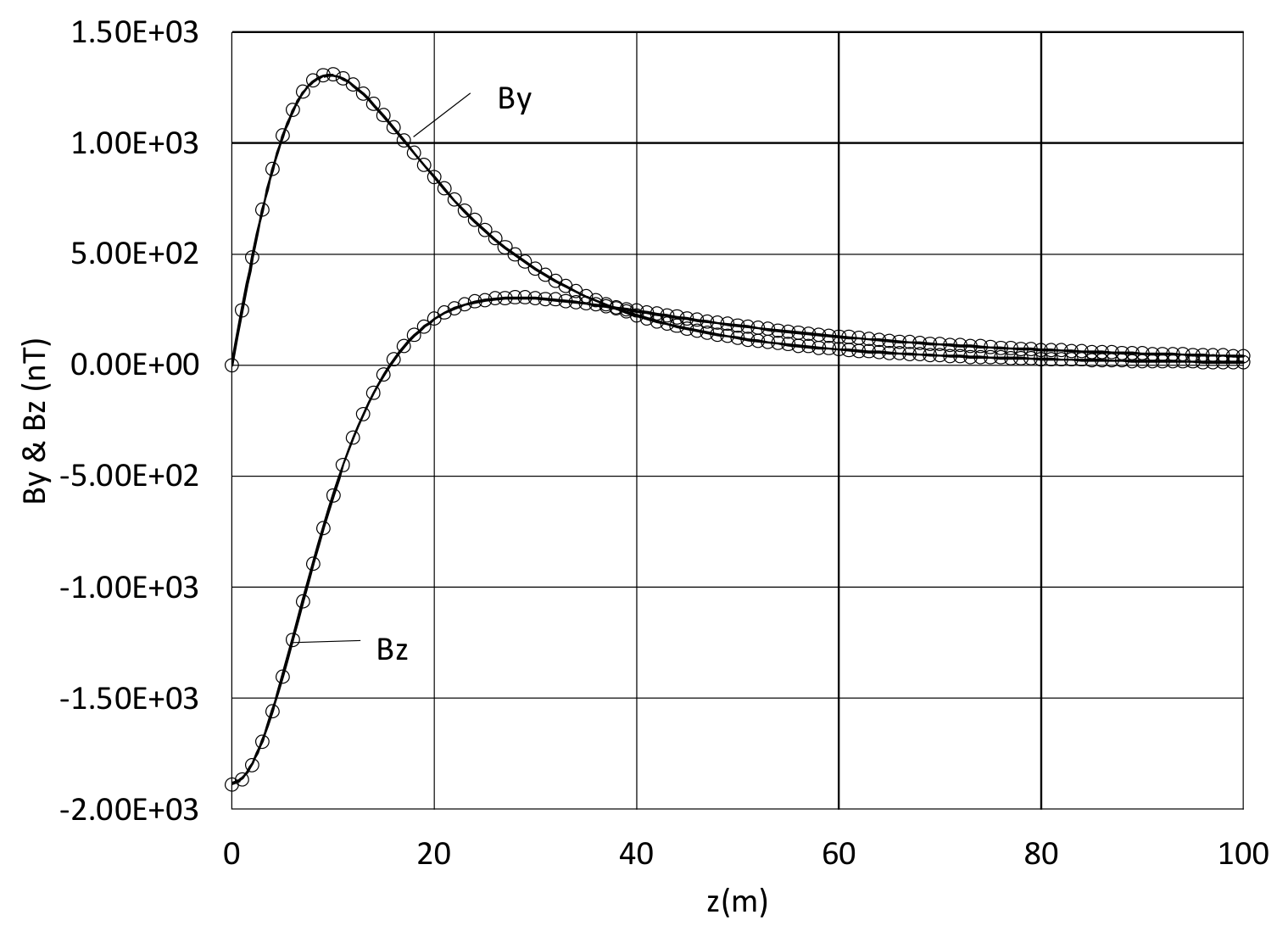
Figure 9.
Longitudinal, Bz and transverse, Bρ (all positive) components of induced field from the axisymmetric ellipsoidal shell of b = c = 10 m in the uniform field of 5.5E4 nTesla at ρ = 20 m: solid line = solution (45),(47) for tρ = 0.02 m; o = solution (25)-(26) for non-confocal ellipsoids & FEA [5] at t = 0.02 m : a = 20 m (1); 50 m (2); 100 m (3).
Figure 9.
Longitudinal, Bz and transverse, Bρ (all positive) components of induced field from the axisymmetric ellipsoidal shell of b = c = 10 m in the uniform field of 5.5E4 nTesla at ρ = 20 m: solid line = solution (45),(47) for tρ = 0.02 m; o = solution (25)-(26) for non-confocal ellipsoids & FEA [5] at t = 0.02 m : a = 20 m (1); 50 m (2); 100 m (3).
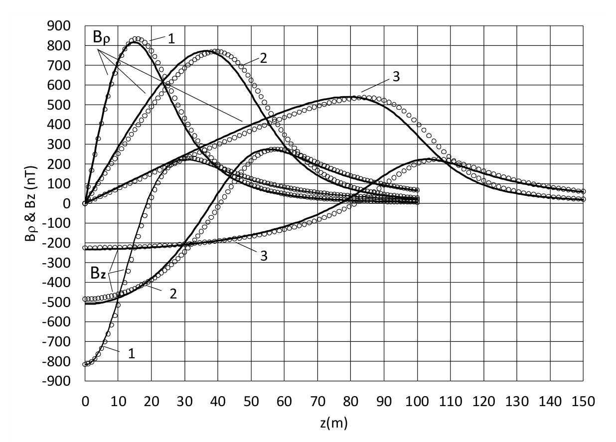
Figure 10.
Transverse, Bρ component of induced field from the axisymmetric ellipsoidal shell of b = c = 10 m in the uniform field of 5.5E4 nTesla: solid line = solution (45),(47) at tρ = 0.04 m; o = solution(25)-(26) for non-confocal ellipsoids & FEA [5] at t = 0.04 m : a = 20 m and ρ = 20 m (1); a = 50 m and ρ = 20 m (2); a = 100 m and ρ = 20 m (3); a = 20 m and ρ = 30 m (4); a = 50 m and ρ = 30 m (5); a = 100 m and ρ = 30 m (6).
Figure 10.
Transverse, Bρ component of induced field from the axisymmetric ellipsoidal shell of b = c = 10 m in the uniform field of 5.5E4 nTesla: solid line = solution (45),(47) at tρ = 0.04 m; o = solution(25)-(26) for non-confocal ellipsoids & FEA [5] at t = 0.04 m : a = 20 m and ρ = 20 m (1); a = 50 m and ρ = 20 m (2); a = 100 m and ρ = 20 m (3); a = 20 m and ρ = 30 m (4); a = 50 m and ρ = 30 m (5); a = 100 m and ρ = 30 m (6).
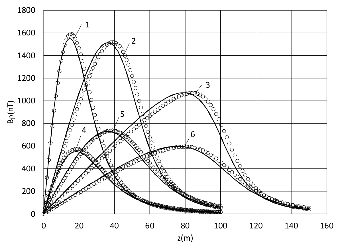
Figure 11.
Longitudinal Bz component of induced field from the axisymmetric ellipsoidal shell of b = c = 10 m in the uniform field of 5.5E4 nTesla for the same data and notations as in Figure 10.
Figure 11.
Longitudinal Bz component of induced field from the axisymmetric ellipsoidal shell of b = c = 10 m in the uniform field of 5.5E4 nTesla for the same data and notations as in Figure 10.
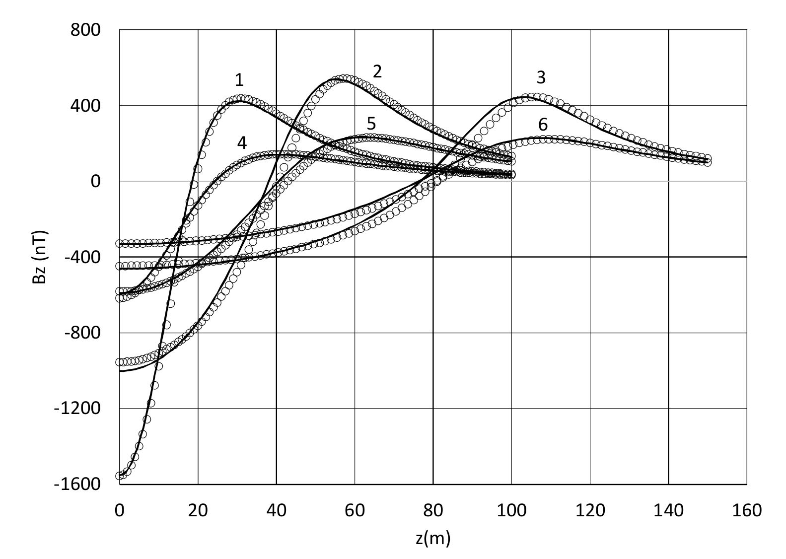
Figure 12.
Longitudinal Bx and transverse (all positive) By & Bz components of induced field of triaxial ellipsoidal shell of a = 20 m, b = 10 m, c = 5 m (labeled by numbers 1-4) and a = 50 m, b = 10 m, c = 5 m (labeled by numbers 5-8) in the uniform field of 5.5E4 nTesla in comparison to the magnetic signature of hollow ellipsoid with the constant wall thickness: By (1,5) and Bx (3,7) at y = 20 m & z=0; Bz (2,6) and Bx (4,8) at z = 20 m & y=0; solid line = solution (29)-(33) at the thicknesses defined per (59); o = FEA [9] for the shell with the equal wall thickness of t=0.02 m.
Figure 12.
Longitudinal Bx and transverse (all positive) By & Bz components of induced field of triaxial ellipsoidal shell of a = 20 m, b = 10 m, c = 5 m (labeled by numbers 1-4) and a = 50 m, b = 10 m, c = 5 m (labeled by numbers 5-8) in the uniform field of 5.5E4 nTesla in comparison to the magnetic signature of hollow ellipsoid with the constant wall thickness: By (1,5) and Bx (3,7) at y = 20 m & z=0; Bz (2,6) and Bx (4,8) at z = 20 m & y=0; solid line = solution (29)-(33) at the thicknesses defined per (59); o = FEA [9] for the shell with the equal wall thickness of t=0.02 m.
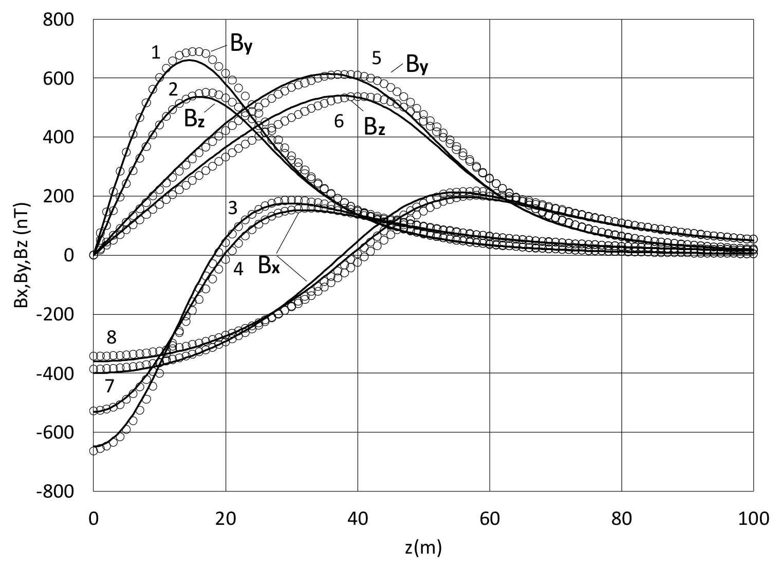
Figure 13.
Longitudinal Bx and transverse (all positive) components By & Bz of induced field of triaxial ellipsoidal shell of a = 50 m b = 10 m, c = 5 m in the uniform field of 5.5E4 nTesla in comparison to the magnetic signature of hollow ellipsoid with the constant wall thickness: By (1) and Bx (3) at y = 20 m & z=0; Bz (2) and Bx (4) at z = 20 m & y=0 ; solid line = solution (29)-(33) at the thicknesses defined per (59); o = FEA [9] for the shell with the equal wall thickness of t=0.04 m.
Figure 13.
Longitudinal Bx and transverse (all positive) components By & Bz of induced field of triaxial ellipsoidal shell of a = 50 m b = 10 m, c = 5 m in the uniform field of 5.5E4 nTesla in comparison to the magnetic signature of hollow ellipsoid with the constant wall thickness: By (1) and Bx (3) at y = 20 m & z=0; Bz (2) and Bx (4) at z = 20 m & y=0 ; solid line = solution (29)-(33) at the thicknesses defined per (59); o = FEA [9] for the shell with the equal wall thickness of t=0.04 m.
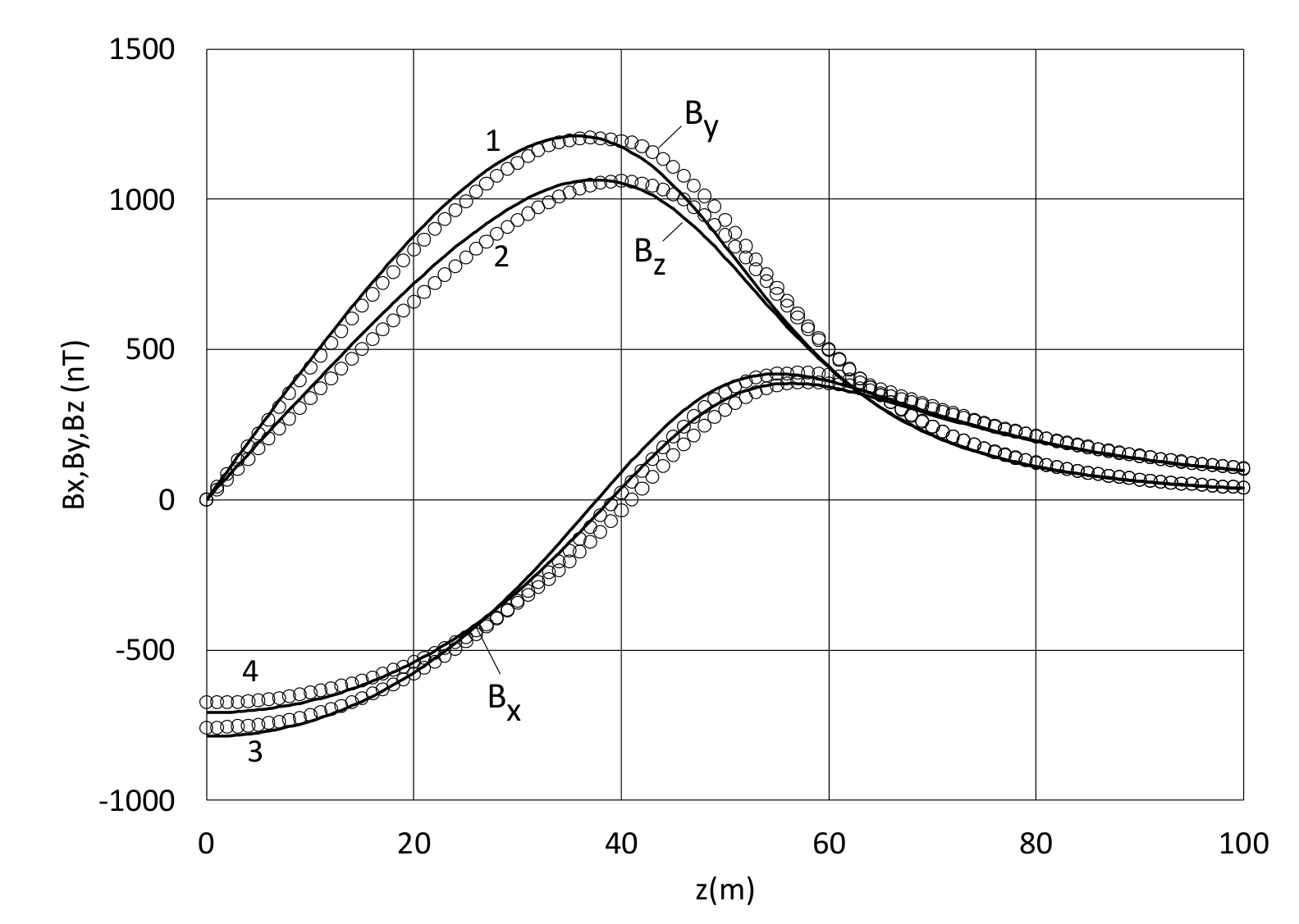
Figure 14.
Logarithmic shielding effectiveness of a thin wall shell of ty = 0.02 and b = 1.5; c = 1 in the longitudinal field Hx for different values of largest semi axis: a = 2,3,4,5,7,10; solid line = analytical solution (64); o = approximation(67) ; ∆ = spherical shell of radius = 1.5 and thickness of 0.0217.
Figure 14.
Logarithmic shielding effectiveness of a thin wall shell of ty = 0.02 and b = 1.5; c = 1 in the longitudinal field Hx for different values of largest semi axis: a = 2,3,4,5,7,10; solid line = analytical solution (64); o = approximation(67) ; ∆ = spherical shell of radius = 1.5 and thickness of 0.0217.
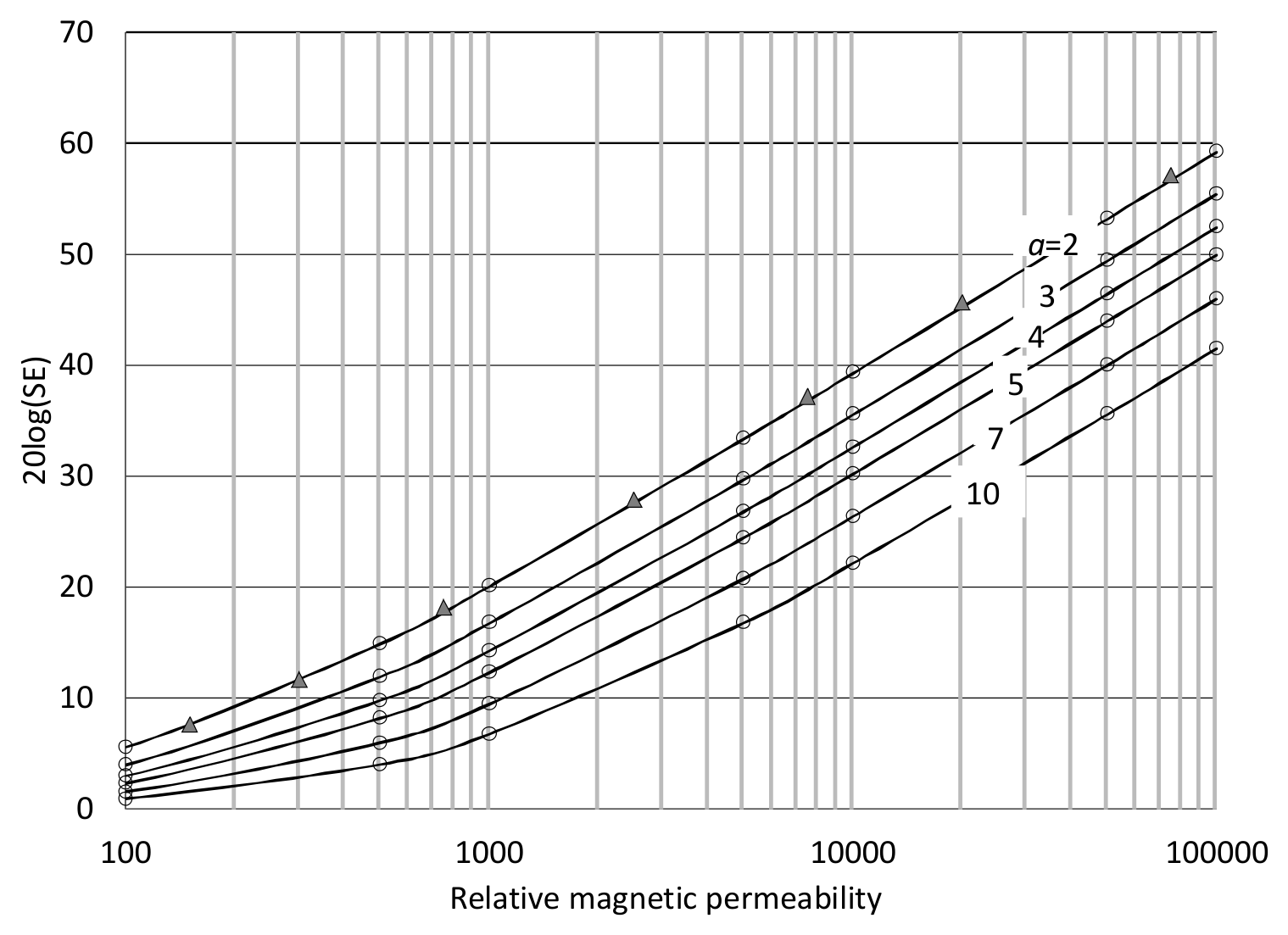
Figure 15.
Logarithmic shielding effectiveness of ellipsoidal shell with a thick wall of ty = 0.2 and b = 1.5; c = 1 in the longitudinal field Hx for different values of largest semi axis: a = 2,3,4,5,7,10; solid line = analytical solution (64); -o- = approximation (67); ∆ = spherical shell of radius =1.5 and thickness of 0.227.
Figure 15.
Logarithmic shielding effectiveness of ellipsoidal shell with a thick wall of ty = 0.2 and b = 1.5; c = 1 in the longitudinal field Hx for different values of largest semi axis: a = 2,3,4,5,7,10; solid line = analytical solution (64); -o- = approximation (67); ∆ = spherical shell of radius =1.5 and thickness of 0.227.
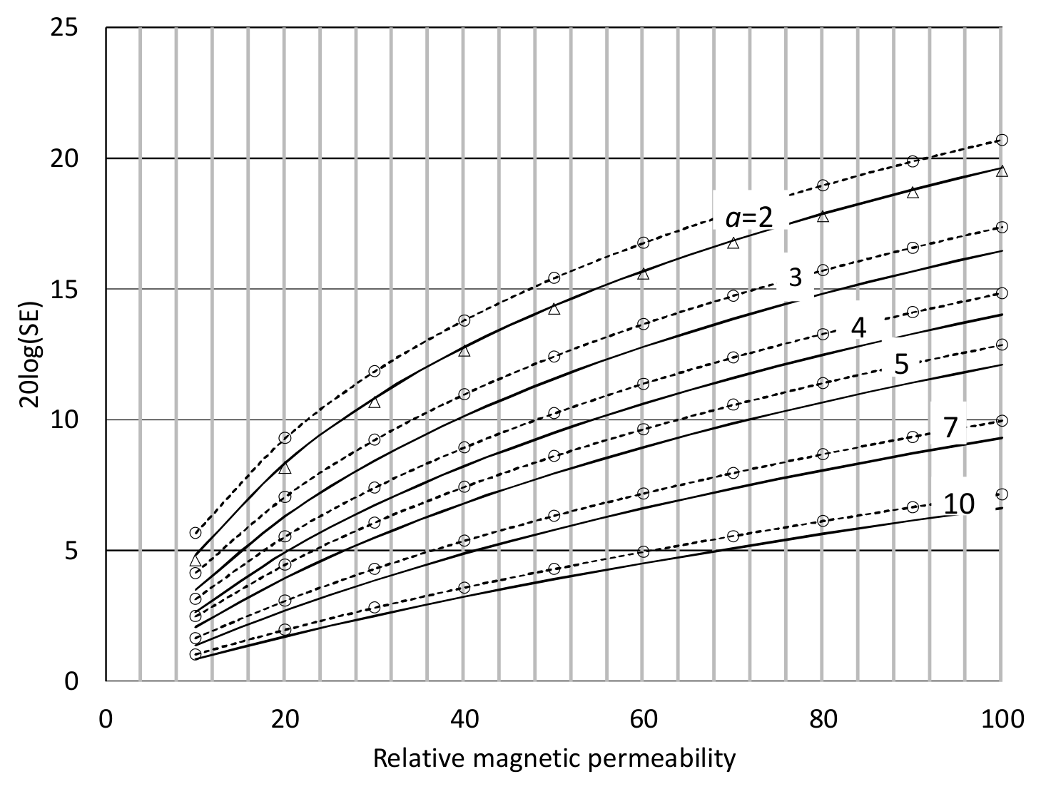
Figure 16.
Logarithmic shielding effectiveness of ellipsoidal shell of b = 1.5; c = 1and ty = 0.02 in the transverse field Hz for different values of largest semi axis: a = 2,10; solid line = analytical solution (64); o = approximation(67); ∆ and x = spherical and cylindrical shells of radius =1.5 and thickness of 0.0217, respectively.
Figure 16.
Logarithmic shielding effectiveness of ellipsoidal shell of b = 1.5; c = 1and ty = 0.02 in the transverse field Hz for different values of largest semi axis: a = 2,10; solid line = analytical solution (64); o = approximation(67); ∆ and x = spherical and cylindrical shells of radius =1.5 and thickness of 0.0217, respectively.
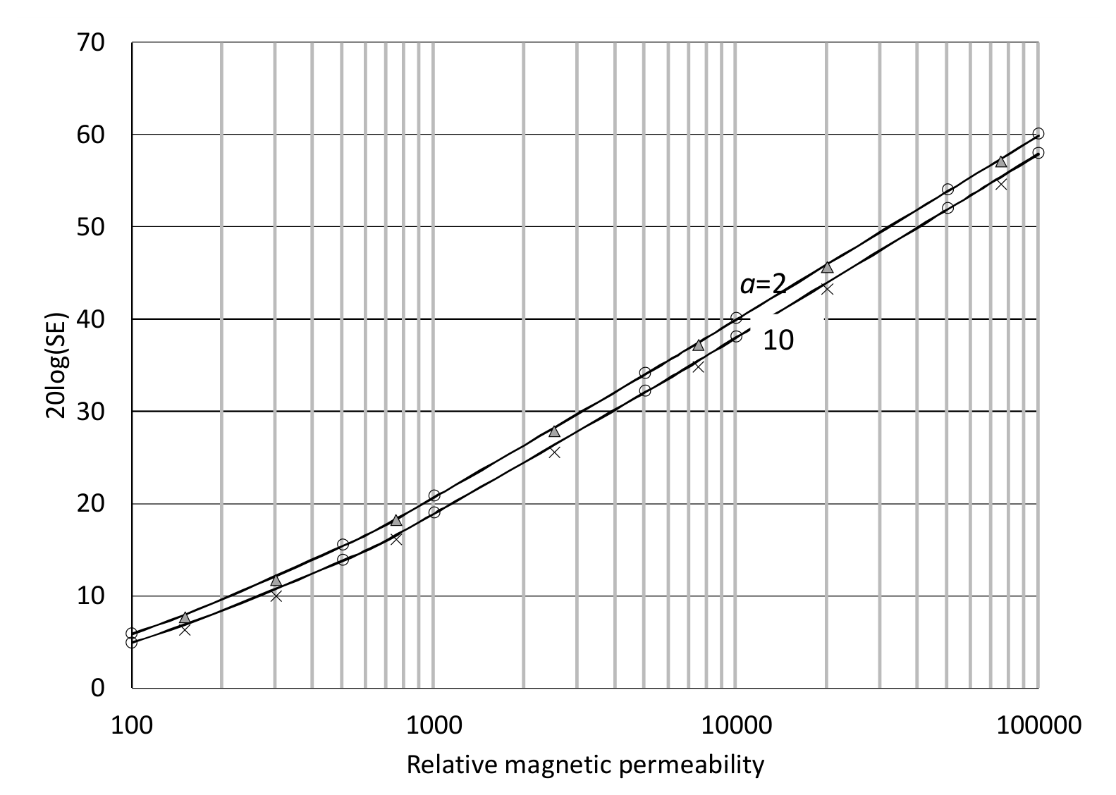
Figure 17.
Demagnetizing field Hdx /H0 of ellipsoidal shell of b = 1.5,c =1 and ty = 0.02 in the longitudinal applied field.
Figure 17.
Demagnetizing field Hdx /H0 of ellipsoidal shell of b = 1.5,c =1 and ty = 0.02 in the longitudinal applied field.
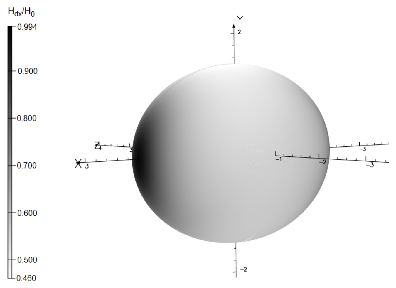
Figure 18.
Averaged demagnetizing field of ellipsoidal shell (ty=0.02) of b=1.5; c=1 at x=0 in the longitudinal applied field Hx for different values of largest semi axis: a = 2,3,4,5,7,10. Solid line = analytical solution (70); -o- = approximation (72).
Figure 18.
Averaged demagnetizing field of ellipsoidal shell (ty=0.02) of b=1.5; c=1 at x=0 in the longitudinal applied field Hx for different values of largest semi axis: a = 2,3,4,5,7,10. Solid line = analytical solution (70); -o- = approximation (72).
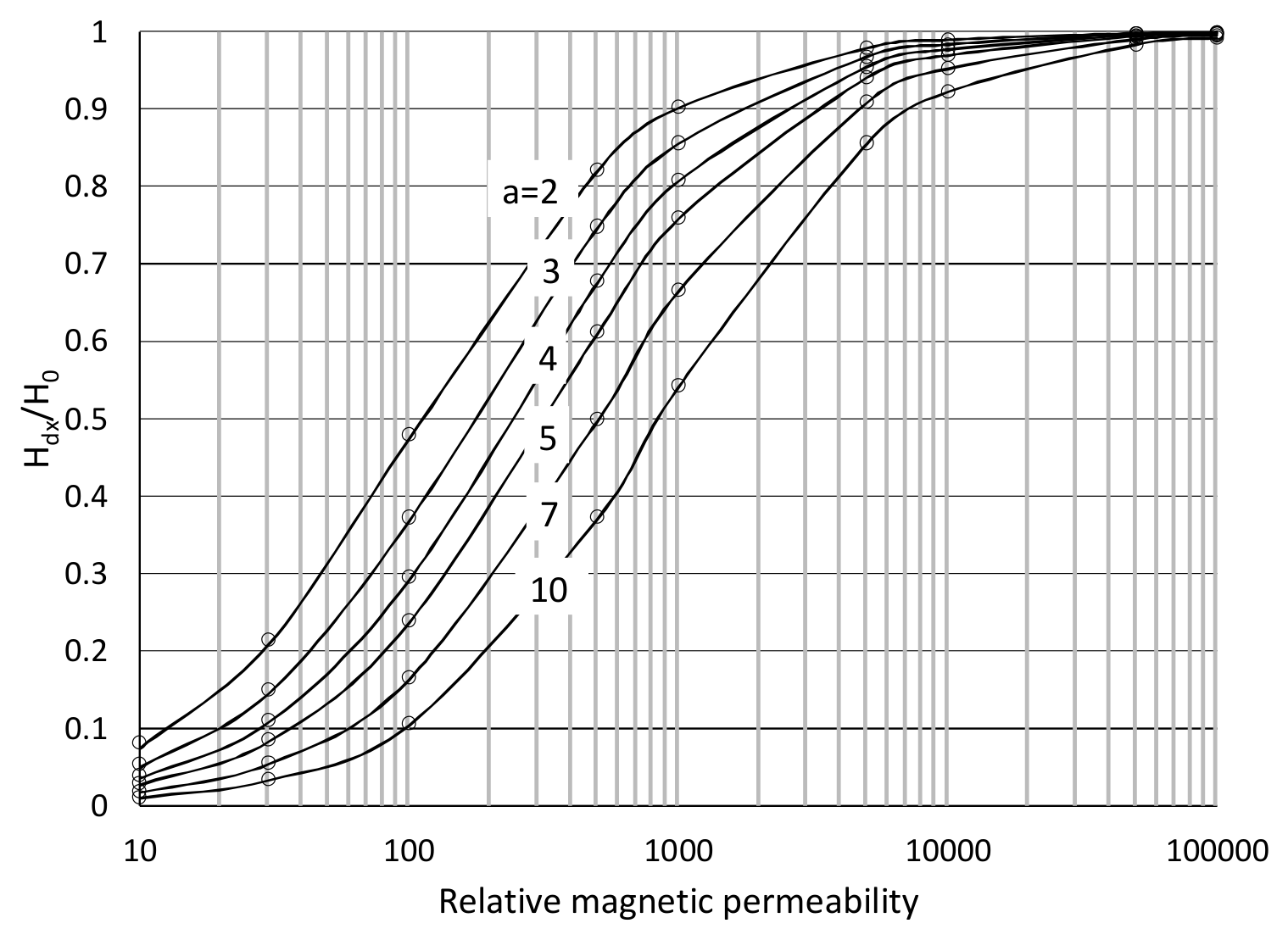
Figure 19.
Longitudinal Bz (3,4) and transverse (1,2) components Bρ of induced field from an axisymmetric ellipsoidal shell in the uniform field of 5.5E4 nTesla at b = c =10 m, tz= 0.02: solid line = analytical solution (45),(47) ;× = dipole approximation; a = 20 m & ρ=100m (1,3); a= 50 m & ρ = 200m (2,4).
Figure 19.
Longitudinal Bz (3,4) and transverse (1,2) components Bρ of induced field from an axisymmetric ellipsoidal shell in the uniform field of 5.5E4 nTesla at b = c =10 m, tz= 0.02: solid line = analytical solution (45),(47) ;× = dipole approximation; a = 20 m & ρ=100m (1,3); a= 50 m & ρ = 200m (2,4).
Disclaimer/Publisher’s Note: The statements, opinions and data contained in all publications are solely those of the individual author(s) and contributor(s) and not of MDPI and/or the editor(s). MDPI and/or the editor(s) disclaim responsibility for any injury to people or property resulting from any ideas, methods, instructions or products referred to in the content. |
© 2026 by the authors. Licensee MDPI, Basel, Switzerland. This article is an open access article distributed under the terms and conditions of the Creative Commons Attribution (CC BY) license (http://creativecommons.org/licenses/by/4.0/).
Copyright: This open access article is published under a Creative Commons CC BY 4.0 license, which permit the free download, distribution, and reuse, provided that the author and preprint are cited in any reuse.