
Submitted:
29 October 2026
Posted:
30 October 2026
You are already at the latest version
Abstract
Systematic comparisons of the classic airfoil literature with modern codes have been limited less by physics than by the labour of extracting data from scanned charts. This study shows that optical character recognition and an AI agent, working under the author’s direction, can automate this chain: source retrieval, chart calibration, visual data reading, simulation campaigns, quality control and documentation. With this workflow, all 112 section charts of NACA Report 824 and three planform figures of Hoerner’s Fluid-Dynamic Lift were recomputed with XFOIL, MSES and AVL in about 7.5 hours of elapsed time. Lift-curve slopes agree to a median +2.2 % (XFOIL), and the overprediction grows with thickness. Zero-lift angles are too negative in proportion to camber in both codes; transition modelling and tunnel-wall corrections were ruled out as causes. Drag is underpredicted by about 15 % at all Reynolds numbers. The offset vanishes for Ncrit ≈ 5, an effective parameter for surface imperfections or the shared boundary-layer model. Maximum lift is overpredicted, most for thin sections. AVL reproduces Hoerner’s planform data within a few per cent where the flow is attached and the edges are sharp. Automated checks found errors in the source, the codes and the agent’s own work; human verification remains essential.
Keywords:
airfoil aerodynamics
; NACA Report 824
; XFOIL
; MSES
; vortex-lattice method
; wind-tunnel data
; digitisation
; optical character recognition
; AI agent
; reproducibility
1. Introduction
Two compilations still anchor much of practical airfoil and wing aerodynamics. NACA Report 824 [1], republished as the data appendix of Theory of Wing Sections [2,3], gives lift, drag and moment measurements for more than a hundred NACA sections at Reynolds numbers of 3 to , smooth and with standard leading-edge roughness. Hoerner’s Fluid-Dynamic Lift [4,5] and Fluid-Dynamic Drag [6] collect experiments from many facilities into empirical design rules. The NACA four-digit, five-digit and 6-series sections remain in use. The characteristics of the 6-series are still reviewed as a reference for large wind-turbine blades [7], alongside dedicated wind-turbine families such as the Delft DU and Risø airfoils [8,9].
These collections predate the numerical tools now used to design airfoils and wings. Viscous–inviscid interaction codes such as XFOIL [10] and MSES [11,12,13], and vortex-lattice methods such as AVL [14], compute in seconds what the historical tests established over years of wind-tunnel work. Published comparisons of these codes with experiment mostly concern a few sections tested in modern facilities. Coder and Maughmer [15] compared XFOIL 6.96, PROFIL07 and the RANS solver OVERFLOW with Penn State low-turbulence tunnel data for six airfoils. They found that the integral boundary-layer codes predicted drag well in the low-drag regions and that XFOIL frequently overpredicted maximum lift. Eisele and Pechlivanoglou [16] compared XFOIL, MSES and RANS with TU Berlin measurements on two wind-turbine airfoils and a slatted configuration at . Both integral boundary-layer codes underestimated the pre-stall drag, which the authors attributed to the boundary-layer formulation. For the 30 %-thick DU 97-W-300 they had to lower the transition criterion to to obtain realistic results. Morgado et al. [17] compared XFOIL with RANS for high-lift, low-Reynolds-number airfoils, and Kallstrom [18] compared XFOIL and OVERFLOW with legacy airfoil tables and wind-tunnel data for rotorcraft airfoil tables. How much a single well-known section’s measurements vary between facilities is shown by McCroskey’s assessment of NACA 0012 data from more than 40 wind tunnels [19]. A targeted search found no systematic recomputation of the complete TR-824 collection, but no priority claim is made here. A designer who uses XFOIL to extrapolate beyond a measured polar has little systematic information on how the code’s errors depend on section family, thickness, camber, Reynolds number or surface condition. Known shortcomings, such as drag underprediction for thick sections [16,20] and the lack of a roughness model [21], are documented for individual cases rather than across a large historical data set.
Why has this gap persisted? Not because the comparison is difficult in principle, but because it is laborious: the data exist only as scanned charts and tables, and a systematic replication requires reading hundreds of pages, building geometry for every section, running and supervising about a thousand viscous polars, and checking each result against its source. Done by hand, this is months of skilled work.
The key novelty of this paper is therefore not the comparison itself, which could have been made at any time since the codes became available, but the way it was made. Data extraction from chart images has been automated before, with deep-learning pipelines for scatter plots [22] and general charts [23]. Interactive digitisers such as WebPlotDigitizer give reliable values between independent coders [24,25]. More recently, multimodal large language models have been used to build datasets from archival scans [26] and, in agentic systems, to extract data from the text and figures of the scientific literature [27]. The search found no application of these techniques to the historical aerodynamic literature. Here optical character recognition [28] and an AI agent working under the author’s direction automated the complete chain: source retrieval, text extraction, page indexing, chart calibration, visual reading of the data, geometry generation, the simulation campaigns, quality control, statistics and figure production. Work that was previously impractical at this scale became a matter of hours (Section 2.1). Every standard chart of TR-824 (112 sections) and three planform figures of Fluid-Dynamic Lift are reproduced with XFOIL 6.99, MSES 3.07 and AVL 3.52, and the computed results are drawn onto the original charts. Where simulation and experiment disagree, the controlling parameters (transition amplification factor, transition location) were varied. Where a mismatch remained, its dependence on section geometry was analysed to identify its cause.
The contributions are:
- 1.
- a demonstration, with documented provenance, quality control and error reporting, that OCR and AI-agent automation can turn a classic printed data collection into a machine-readable, code-validated benchmark (Section 2.1);
- 2.
- a complete, page-by-page replica of the TR-824 section data with XFOIL and MSES results drawn on the original charts (Supplementary File S1);
- 3.
- digitised data sets of the TR-824 summary figures, chart legends, ordinate tables, selected drag polars and three Hoerner planform figures, with the geometry, polars and scripts used;
- 4.
- statistics of code-versus-experiment error for zero-lift angle, lift-curve slope, maximum lift and drag, their trends with thickness, camber and roughness, and physical explanations for the remaining discrepancies.
2. Materials and Methods
2.1. An OCR- and AI-Agent-Based Replication Workflow
Replicating TR-824 and Hoerner by hand would require locating and reading hundreds of chart pages, transcribing ordinates and legends, building geometry, running and supervising about a thousand viscous polar computations, and checking every result against its source. Each step is routine; together they amount to months of skilled work, which is why such systematic replications are rarely undertaken. This section describes how the work was instead carried out by an AI agent under the direction of the author, within about seven and a half hours of elapsed time from the first instruction to the first complete draft (session log, including literature review and installing the codes).
2.1.1. Division of Labour
The agent was Claude Code (Anthropic), an agentic AI assistant that runs shell commands, writes and executes code, reads images and documents, and searches the web and the author’s document archive, all inside an isolated Linux container. The underlying model was Claude Opus 5.5. The author set the research goals, provided access to the sources, took the decisions that required judgement (e.g. how to treat MSES stall), and reviewed the results. The agent:
- retrieved the sources (the TR-824 scan from the NASA Technical Reports Server, the Hoerner scan from the author’s archive) and built and validated the codes (XFOIL, MSES, AVL) from source;
- extracted the text of both documents, using the text layer of the TR-824 scan (Poppler pdftotext 24.02) and Tesseract 5.3.4 [28] on 300-dpi renderings of all 507 Hoerner pages;
- indexed all 128 TR-824 chart pages and identified the 112 standard section charts;
- wrote the image-processing code that deskews each chart page, detects its two chart frames and calibrates the axes from the frame lines (Section 2.2);
- read the data visually from calibrated, magnified crops of the scans, using its multimodal (vision) capability, with pixel-to-value conversion by the calibration code;
- generated the geometry, ran and monitored the XFOIL, MSES and AVL campaigns, and restarted or repaired failed runs;
- computed the statistics, drew the figures and overlays, and drafted the manuscript. In the manuscript, every number is a macro generated from the analysis files, and every reference was checked against Crossref, OpenAlex, NTRS or the title page of the copy used.
2.1.2. Scale
2.1.3. Quality Control and Errors Found
Automation at this scale only adds value if errors are found. The agent ran consistency checks at every stage. Errors in the sources, the codes and its own work came to light, all of which are documented with the data:
- Source errors. A misprinted ordinate in the TR-824 table of NACA 63(420)-422 (“3.98” for 0.398, Section 2.2), and a non-constant offset between printed and PDF page numbers in the TR-824 data section.
- Code and tool errors. XFOIL 6.996 failing to converge on NACA 0012 and writing incorrect transition locations; XFOIL silently truncating file paths near 64 characters; folded contours in generated 6-series coordinates, which gave NaN drag; a corrupt regenerated Orr–Sommerfeld amplification map in the MSES build; an MSES polar with a non-physical lift jump (Section 2.3).
- Errors of the agent. In the first fixed-transition campaign the agent placed the XFOIL trips at without checking that they were active. As a result, 80 % of the points were not tripped on one surface. The error was found only while the manuscript was being drafted, when kinks in the computed drag polars were traced to their cause. All affected polars were recomputed, and the check is now part of the analysis. Earlier drafts of the bibliography also contained wrong author names and page references, which the verification step corrected.
The visual readings were spot-checked against an independent source. An independent digitisation of the NACA 4415 lift curves from the author’s archive gives and . The agent read from report Figure 37 and 1.57 from Figure 39 (stated reading uncertainties and ). The maximum lift agrees within the reading uncertainty. The zero-lift angles differ by , more than the stated uncertainty. Part of this difference may come from comparing a summary figure with an interpolated lift curve. In addition, the author checked all figures by hand against the original charts, and the computed statistics against the results of his own earlier studies; no discrepancies were found.
2.1.4. Why This Matters
The comparisons in Section 3.1 and Section 3.2 could in principle have been made at any time in the last three decades. What is new is the cost: the complete replication of a classic data report, with page-level visual comparison, statistics, parameter studies and documented provenance, became a task of hours rather than months. The same workflow applies directly to other historical collections, such as the remaining NACA and AGARD reports, and to Hoerner’s Fluid-Dynamic Drag. This opens the possibility of systematically turning the pre-digital literature into machine-readable, code-validated benchmarks. The remaining human tasks are to direct the work, to check that it is correct, and to interpret what it shows.
2.2. Historical Sources and Their Digitisation
2.2.1. NACA Report 824
The airfoil data are taken from Abbott, von Doenhoff and Stivers, Summary of Airfoil Data, NACA Report 824 [1], the report whose data appendix was republished in Theory of Wing Sections [2,3]. The NASA Technical Reports Server scan (record 19930090976; 261 pages, 300 dpi bilevel images with a hidden OCR text layer) was used throughout. In the text part of the report (PDF pp. 6–65), printed page numbers equal PDF page numbers minus five, and printed pages are cited. In the data section the printed numbers are not a constant offset from the PDF (PDF p. 134 is printed p. 132, PDF p. 260 is printed p. 264), so data pages are cited by PDF page.
The data section (“Aerodynamic characteristics of various airfoil sections”, PDF pp. 133–260) contains 128 chart pages: 112 standard section charts (lift and quarter-chord moment versus angle of attack; drag and moment about the aerodynamic centre versus lift coefficient), 13 pages for sections with flaps and three drawings. Each title was checked visually by the AI agent (Section 2.1) and recorded in a page index. The standard charts contain data at nominal Reynolds numbers , 6 and and, for most sections, with standard leading-edge roughness at . The actual test Reynolds numbers and the measured aerodynamic-centre positions printed in every chart legend were transcribed for all 112 charts.
The models were 24-in chord and were tested in the Langley two-dimensional low-turbulence tunnels, whose turbulence level the report gives as “only a few hundredths of 1 percent” (printed p. 54). Standard roughness is defined as 0.011-in carborundum grains over from the leading edge on both surfaces, covering 5–10 % of that area (printed p. 24). The rough data remain relevant to present-day designs. On the NACA 4415, a grit pattern derived from insect contamination measured on wind-turbine blades [29] produced nearly the same loss of performance as standard roughness, and standard-roughness tests have therefore been recommended as the worst case in wind-turbine blade design [21].
Digitisation tiers.
Three levels of extraction were used.
- 1.
- Tier A, page overlays. Each chart page is deskewed, both chart frames are detected, and the axes are calibrated from the frame lines (each frame spans 32 grid cells horizontally and 56 vertically). Computed curves are drawn directly on the faded scan, so every one of the 112 sections can be compared visually in its original presentation (Supplementary File S1).
- 2.
- Tier B, summary figures. Zero-lift angles (report Figure 37, 95 sections), faired lift-curve slopes versus thickness (Figure 38, five families, smooth and rough) and maximum lift versus thickness (Figure 39, smooth and rough) were read by the agent on calibrated, magnified grids. Grid-line spacings measured in the scans deviate from uniform axes by at most about px (about 3 % of a grid cell).
- 3.
- Tier C, drag polars. Faired drag polars at fixed for all four test conditions were read for eight sections (NACA 0009, 2412, 4415, 23012, -415, -618, -415, -415). The reading uncertainty is in .
Automatic symbol recognition was attempted and abandoned: at 300 dpi the plotted symbols are 6–15 px across, overlap grid lines and each other, and could not be classified reliably. The data were therefore read visually by the agent from magnified crops, point by point, and every reading records its uncertainty.
Geometry.
Coordinates for 102 sections were generated with NACA456 [30], which implements the procedures of NASA TM-4741 [31]. They reproduce NACA456’s own surface ordinates to , and spot checks against UIUC database files agree within . Sections with a parenthesised base thickness, e.g. 63(420)-422, were scaled linearly from the base form, as the report prescribes (printed pp. 5–6).
Two cases required the report’s own ordinate tables. Sections designated with a comma, e.g. -618, are the earlier individually derived airfoils whose ordinates the report states are “slightly different” from those of the later subscript family (printed p. 6). The 7-series sections are not supported by NACA456. The ordinates of these ten sections were transcribed visually by the agent from the tables (PDF pp. 105, 109 and 114). One table misprint was found and corrected: the second upper-surface station of 63(420)-422 is printed as “3.98” and must read for the stations to increase monotonically. The NACA456 approximations differ from the tables by 0.03–0.09 %c for the and sections but by about 0.5 %c for -420 and 63(420)-422.
2.2.2. Hoerner, Fluid-Dynamic Lift
The second edition [5] was used (title page: second edition, 1985, published by Mrs. Liselotte A. Hoerner; H. V. Borst co-author and editor). The 507-page scan was OCR’d page by page. Three planform figures that potential-flow theory should reproduce were digitised by the agent on axes calibrated from their tick marks (300 dpi): Figure 3-2 (lift angle versus , 29 points), Figure 15-9 (lift-curve slope of swept wings, –6, 29 points) and Figure 17-3 (linear lift-curve slope of low-aspect-ratio wings and plates, 53 points). Because the book’s copyright notice forbids reproduction of its illustrations without permission, Hoerner’s data appear here only as re-plotted digitised values.
2.3. Numerical Methods
2.3.1. Section Analysis: XFOIL and MSES
XFOIL 6.99 [10,12] couples a linear-vorticity panel method to an integral boundary layer with envelope transition. Each section was repanelled to 240 nodes by curvature. Polars were computed as two sweeps starting at : upward to in steps and downward to in steps, with 120 Newton iterations per point. XFOIL does not recover once a point diverges, so a stalled sweep was restarted in a fresh process beyond the last converged point, up to four times per direction; where values overlapped, the continuation points were kept. The newer release XFOIL 6.996 was not used: on NACA 0012 at it failed to converge at and wrote incorrect transition locations to its polar file, whereas 6.99, built identically, converged throughout.
MSES 3.07 [11,12,13] solves the Euler equations on a streamline grid coupled to the same family of integral boundary-layer closures. Grids were generated with the parameters of the RAE 2822 example distributed with the code, at . MPOLAR sweeps from to and were restarted beyond the last converged point with steps. The build was verified on RAE 2822 case 6 (, , ): and , against and measured.
Case matrix.
For each of the 112 sections, XFOIL was run at , 6 and with ; at with and 13; and at with transition fixed on both surfaces as a proxy for standard roughness. For the eight Tier-C sections, and 7 were added at . MSES was run at with , free transition and transition fixed at ; for the replica pages (Supplementary File S1) it was also run at and with free transition. In total 688 XFOIL and 448 MSES polars were computed. Of these, 0 XFOIL and 23 MSES polars contain no converged point.
Choice of .
The XFOIL user primer [32] recommends –12 for a “clean wind tunnel” and 9 for an “average” one. Given the turbulence level reported for the Langley low-turbulence tunnels, was adopted as the baseline, with 9 and 13 as sensitivity cases. In earlier clean-model measurements on a wind-turbine section at , gave the best agreement with the measurements [21].
Roughness proxy.
In XFOIL a trip is ignored once it lies upstream of the stagnation point, because the boundary layer of that surface then starts aft of it. The solution silently reverts to free transition, as the polar’s transition columns show. In a first campaign with trips at this happened on the pressure side from –, and 80 % of the points were affected. The XFOIL trips were therefore placed at , still inside the roughness band. Even this trip is passed by the stagnation point above . Every computed point is therefore checked: lift quantities use points at which the suction-side trip is active, drag uses points at which both trips are active. In MSES the transition point of the pressure side follows the stagnation point aft, so its trip remains effective. Fixing transition near the leading edge reproduces the transition effect of standard roughness but neither the roughness-induced increase in skin friction nor the thickening of the initial boundary layer. The resulting bias is quantified in Section 4.
2.3.2. Extraction of Section Characteristics
The same definitions were applied to every computed polar:
- : zero crossing of , by linear interpolation;
- : least-squares slope over ;
- , over the same range;
- : maximum of the upward sweep, accepted only if stall was reached, i.e. falls by at least 0.02 after the peak, or the local slope over the last before the peak is below 10 % of . A peak approached with a slope above over the preceding is rejected as non-physical. This removes one MSES polar (NACA 23018) in which jumps to 2.26. Sweeps that ended on the linear branch are excluded from the statistics.
2.3.3. Planform Analysis: AVL
AVL 3.52 [14] is a vortex-lattice method. Flat planar wings were modelled with 16 chordwise (cosine) by 40 spanwise (sine) vortices per half span. The section lift-slope factor CLAF (2D slope relative to ) was set to 1.0 and 0.9. The lift-curve slope was taken from AVL’s stability-axis derivative . Planforms were rectangular, linearly tapered () and elliptic, with –20, and swept straight-tapered wings with –6 and to . On a rectangular wing, AVL agreed within 1.5 % with two independent vortex-lattice codes (an in-house horseshoe solver and AeroSandbox).
3. Results
3.1. NACA Report 824
All comparisons are at the nominal Reynolds numbers. The actual test values printed in the chart legends differ from the nominal ones by a few per cent. Errors are given as computed minus measured. Relative errors are medians over sections, which are robust to the few cases in which a computed sweep is incomplete.
3.1.1. Zero-Lift Angle
Figure 1 compares computed zero-lift angles with the 95 values of report Figure 37. Both codes predict too negative: XFOIL by -0.21° on average (rms 0.32°, ) and MSES by -0.18° (rms 0.29°, ). The two codes agree with each other far more closely than either agrees with the experiment. The error grows with camber (Table 2): it is negligible for symmetrical sections and reaches -0.64° (XFOIL) for the sections whose design lift coefficient is 0.6.
3.1.2. Lift-Curve Slope
Figure 2 compares the lift-curve slope with the faired curves of report Figure 38. TR-824 observes that the slope of the four- and five-digit sections decreases with thickness, whereas that of the 6-series sections increases with thickness [printed p. 30 [1]. Both codes reproduce the increase for the 6-series. Neither reproduces the decrease for the older families, for which the computed slope stays near or above the thin-airfoil value. The median overprediction is +2.2 % for XFOIL () and +3.8 % for MSES (), and it grows with thickness (Table 2). With standard roughness the measured slopes of thick sections fall well below the smooth values. With transition fixed at , XFOIL overpredicts the rough slope by a median +4.8 %.
3.1.3. Maximum Lift
Maximum lift is the least reliable computed quantity (Figure 3). For smooth sections XFOIL overpredicts by a median +16.6 % ( sections with a resolved stall). MSES resolved stall for only 16 sections, because its Newton solver usually stops converging at stall onset. For these, the median error is +3.2 %, with a wide spread. For example, MSES predicts an abrupt leading-edge stall for the 9 %-thick 65- and 66-series sections at , the correct stall type but at a lift coefficient about 0.25 too low. With standard roughness the measured drops by a median of 0.30 (up to 0.49; 67 thickness–camber pairs of Figure 39). Leading-edge transition captures only a small part of this drop: the median overprediction is +56.1 % for XFOIL () and +34.1 % for MSES ().
3.1.4. Drag
Drag polars were compared for the eight Tier-C sections (Figure 5). With free transition and , XFOIL underpredicts the drag by a median -15.9, -14.7 and -15.2 % at , 6 and . The offset is therefore almost independent of Reynolds number. MSES gives -17.5, -15.3 and -16.4 % at the same Reynolds numbers. The low-drag bucket of the 6-series sections is reproduced qualitatively: its corners lie at about the measured lift coefficients, but the computed bucket floor is too low. With standard roughness the computed drag is -23.4 % below the measurements ( points at which both trips are active).
Figure 3.
Maximum section lift coefficient against thickness ratio at : TR-824 Figure 39 (one line per camber group) and computed values. Only polars in which stall was resolved are shown (Section 2.3). Top: smooth; bottom: standard roughness (XFOIL: transition fixed at ; MSES: ).
Figure 3.
Maximum section lift coefficient against thickness ratio at : TR-824 Figure 39 (one line per camber group) and computed values. Only polars in which stall was resolved are shown (Section 2.3). Top: smooth; bottom: standard roughness (XFOIL: transition fixed at ; MSES: ).
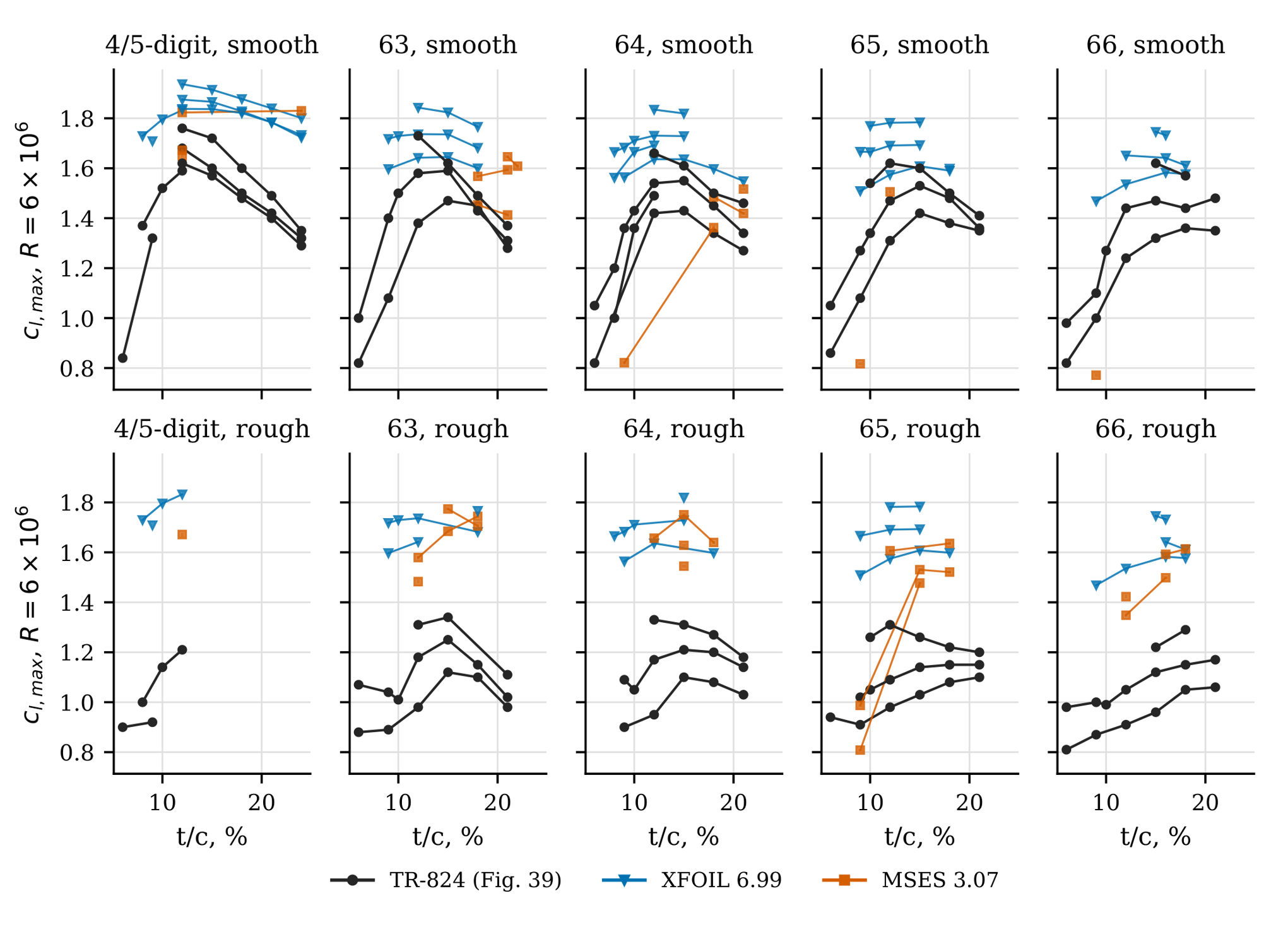
Figure 4.
Lift curve of the NACA 4415 at : an independent digitisation of the Abbott and von Doenhoff data, smooth and with standard roughness, against XFOIL and MSES.
Figure 4.
Lift curve of the NACA 4415 at : an independent digitisation of the Abbott and von Doenhoff data, smooth and with standard roughness, against XFOIL and MSES.
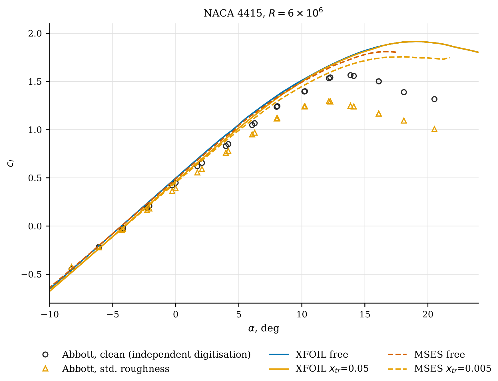
Figure 5.
Section drag polars of the eight Tier-C sections: TR-824 faired values (symbols) and XFOIL (solid; smooth , rough with both trips active) and MSES (dotted).
Figure 5.
Section drag polars of the eight Tier-C sections: TR-824 faired values (symbols) and XFOIL (solid; smooth , rough with both trips active) and MSES (dotted).
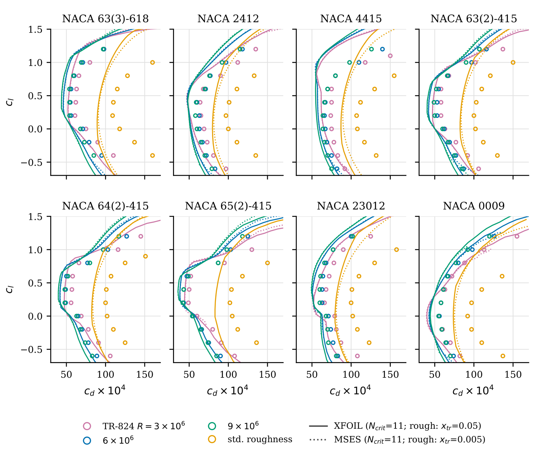

Table 2.
Error trends at , smooth, . : mean error (deg) by first digit of the camber designation (design lift coefficient for the 6-series); slope and : median relative error (%) by thickness class. n in parentheses.
Table 2.
Error trends at , smooth, . : mean error (deg) by first digit of the camber designation (design lift coefficient for the 6-series); slope and : median relative error (%) by thickness class. n in parentheses.
| XFOIL | MSES | |
|---|---|---|
| , symmetrical | -0.02 (25) | -0.03 (25) |
| , camber digit 2 | -0.19 (36) | -0.17 (35) |
| , camber digit 4 | -0.39 (20) | -0.35 (18) |
| , camber digit 6 | -0.64 (4) | -0.58 (4) |
| , –10 % | +1.3 (26) | +1.8 (25) |
| , –15 % | +2.0 (34) | +3.7 (33) |
| , –24 % | +3.6 (43) | +5.4 (42) |
| , –10 % | +25.3 (16) | -23.6 (2) |
| , –15 % | +12.6 (29) | +0.3 (4) |
| , –24 % | +19.5 (18) | +7.8 (10) |
3.2. Hoerner’s Planform Data
Hoerner’s empirical equations are referred to by their numbers in the corresponding chapter of Hoerner and Borst [5]. In every figure, the experimental points are digitised values re-plotted by the authors, not reproductions of the original figures.
3.2.1. Lift Angle Versus Aspect Ratio (Figure 3-2)
Hoerner presents the lift angle against and fits it with Eq. (6), (deg), for rectangular wings with sharp tips, and gives Eq. (7), , as an upper limit for “round” wings with rounded lateral edges or planforms (Figure 6). For –20, AVL (rectangular, CLAF 0.9) lies within to of Eq. (6), close to the sharp-tipped data. The rounded-tip data lie above all AVL curves, including the elliptic planform. Hoerner attributes their penalty to “some flow around the lateral edges”, which reduces both the effective aspect ratio and the effective wing area [5, p. 3-3]. A planar vortex lattice with a fixed tip has no such mechanism. AVL therefore represents the sharp-edged wing.
3.2.2. Swept Wings (Figure 15-9)
Figure 7 compares the lift-curve slope of swept wings with –6 against AVL for (208 cases). With CLAF and , the mean residual per aspect ratio is within per degree (about 4 %). Hoerner’s cosine-law Eq. (17) falls below the data at , whereas AVL follows them. The maximum slope does not occur at zero sweep: Hoerner places this “neutral angle of sweep” at for [p. 15-8 [5], and the largest digitised values for and 6 lie at , although the data are sparse there. On its sweep grid, AVL places the maximum at only for the tapered wing and at otherwise, so the computed shift is smaller than the measured one. The half-span measurements agree with AVL (CLAF ) within per degree for but lie 0.005–0.012 per degree below it at –. This may reflect the wall boundary layer on the reflection plane, which matters more at high sweep; the source does not allow a firmer attribution.
3.2.3. Low Aspect Ratio (Figure 17-3)
At small aspect ratio, AVL recovers slender-wing theory, per radian, i.e. per degree [Hoerner Eq. (7) of Ch. XVII]: 0.0068 against 0.0069 per degree at . The 53 digitised points separate by edge shape (Figure 8). Sharp-edged plates lie a median 4.4 % above AVL, which is consistent with the additional, non-linear lift of the side-edge vortices that a planar vortex lattice omits. Rounded-edge wings lie 7.9 % below AVL, which is consistent with Hoerner’s reduced effective span [Ch. XVII Eq. (9)]. Hoerner’s empirical Eq. (10) fits the sharp-edged data slightly better than AVL (rms 0.0017 against 0.0022 per degree), which is expected of a fit to these data.
4. Discussion: Why the Results Deviate
4.1. Drag: An Offset That Can Absorb
The drag offset is almost the same at all three Reynolds numbers and in all eight sections, so it is a natural target for parameter adjustment. Figure 9 shows the drag error against . The median error falls monotonically from -17.1 % at through -14.7 % (11), -11.7 % (9) and -7.4 % (7) to -3.3 % at . Reproducing the TR-824 drag levels therefore requires . The XFOIL user primer associates this value with a “dirty wind tunnel” (–8) [32]. The Langley tunnels, in contrast, had a turbulence level of “only a few hundredths of 1 percent” [1, printed p. 54].
We therefore read as an effective value that absorbs effects not present in the computation. It is not a statement about the free-stream turbulence. Three candidate effects were examined:
- 1.
- Model surface quality. TR-824 states that reducing waviness to permissible values is harder than achieving the required smoothness, and that the required freedom from waviness is harder to specify [1, printed p. 22]. Its Figure 22 shows the variation of drag with Reynolds number for an NACA 65(421)-420 model “with a small amount of surface waviness” (printed p. 24). Small waves and residual roughness promote earlier transition, which an method can represent only through a lower .
- 2.
- Measurement and correction. Drag was obtained from wake surveys (printed p. 54). The tunnel-wall correction multiplies the measured drag by (Eq. 40, printed p. 59), with (see below) and (printed p. 58). Explaining a 15 % discrepancy would require the shape factor to be about 4. The report also states that the wake-blocking and pressure-gradient effects it neglects are small.
- 3.
- Drag prediction in the code. Ramanujam et al. [20] report XFOIL-type drag underpredictions of up to 30 % for thick wind-turbine airfoils and attribute them to the momentum thickness used in the drag evaluation. Their abstract states that the correction is implemented in recent XFOIL versions; the drag routine (CDCALC) of the public XFOIL 6.996 was found to be identical to that of 6.99. The error found here shows no systematic trend with thickness between 9 and 18 %. It appears equally in MSES, whose median drag error is -17.5, -15.3 and -16.4 % at , 6 and , against -15.9, -14.7 and -15.2 % for XFOIL (Figure 5). This rules out a cause specific to XFOIL’s drag evaluation, and a thickness-specific one for these sections. It does not rule out a cause in the integral boundary-layer formulation that both codes share. Eisele and Pechlivanoglou [16] observed the same pre-stall drag underestimate in XFOIL and MSES at on wind-turbine sections, and attributed it to that formulation. In contrast, Coder and Maughmer [15] found that the integral boundary-layer codes predicted drag well in the low-drag regions of their Penn State data.
Two explanations therefore remain consistent with all observations: residual model surface imperfections in the TR-824 tests, and a shared shortcoming of the integral boundary-layer formulation. The present data cannot separate them. Separating them would require comparison with a RANS solver on the same sections, or modern tests of the same sections with verified surface finish. For reproducing TR-824 drag, –7 is recommended as an effective calibration. Its effect on transition-sensitive quantities other than drag was not examined here. A similar calibration was used by Eisele and Pechlivanoglou [16], who lowered to 2 to obtain realistic XFOIL and MSES results for the 30 %-thick DU 97-W-300.
4.2. Zero-Lift Angle: A Uniform Overestimate of Effective Camber
The error grows in proportion to camber, is the same in XFOIL and MSES, and does not depend on : the mean XFOIL error is for , 11 and 13. Three explanations were tested.
- Tunnel-wall correction. The correction of angle of attack (Eq. 38, printed p. 59) contains the terms and , which the report describes as usually negligible. With (Eq. 32, printed p. 57), a 2-ft chord and a 7.5-ft test section (printed p. 54), . For our sections each term is then at most about , and the two have opposite signs. Neglecting them cannot explain an error of 0.4–.
- Mean-line type. TR-824 reports that measured zero-lift angles are about 0.93 times the thin-airfoil value for four-digit sections, 1.08 times for the 230 series and 0.74 times for 6-series sections with the mean line [printed p. 30 [1]. Measured divided by computed values are much more uniform: 0.880 (four-digit, ), 0.936 (230 series, ) and 0.886 (6-series, ) for XFOIL. The codes therefore capture the dependence on mean-line type that thin-airfoil theory misses. What remains is a nearly uniform proportional excess of effective camber.
- Viscous decambering. A proportional excess of effective camber points to the boundary layer near the trailing edge, whose displacement effect reduces the effective camber. Both codes use the same family of integral closures, and both appear to underestimate this decambering. The same diagnosis, a computed boundary layer that is too thin, is consistent with the drag underprediction. Model contour deviations of the size TR-824 discusses would act in the same sense and cannot be separated from it with these data.
4.3. Lift-Curve Slope: Thickness Effects
Potential flow increases the lift-curve slope with thickness, and the codes follow this trend in all families. The measured four- and five-digit slopes instead decrease with thickness. TR-824 identifies thickness and thickness distribution as the primary variables, and Reynolds number and camber as having no systematic effect (printed p. 30). In both codes the overprediction grows with thickness (Table 2). This is the signature of trailing-edge boundary-layer growth on thick sections with aft adverse pressure gradients, which the codes model but underestimate, as for . The growth is larger in MSES than in XFOIL.
4.4. Maximum Lift: Unmodelled Stall Mechanisms
The error depends on the stall type. Thin sections () stall at the leading edge through laminar-bubble bursting. XFOIL does not capture this mechanism and overpredicts by a median +25.3 %. MSES does produce an abrupt leading-edge stall for the 9 %-thick 65- and 66-series sections, but about 0.25 too early in . Medium-thickness sections are predicted best, with a median XFOIL error of +12.6 %. Thick sections stall from the trailing edge, and their overprediction of +19.5 % is consistent with the underestimated trailing-edge boundary-layer growth discussed above. XFOIL’s tendency to overpredict maximum lift agrees with the findings of Coder and Maughmer [15] for six modern airfoils, and those of Eisele and Pechlivanoglou [16] for the thick DU 97-W-300. The roughness proxy reduces computed much less than the measured roughness does. Leading-edge transition reproduces the loss of laminar flow but not the extra skin friction and momentum deficit created by the 0.011-in grains over [1, printed p. 24]. The same deficit appears in the drag. With both trips active, XFOIL underpredicts the rough drag by -23.4 %, against -14.7 % for the smooth models. The difference of roughly 9 percentage points is the part of the roughness penalty that a trip cannot represent. The same limitation was found in earlier wind-tunnel tests of the AH 93-W-174 at , clean and with dense grit roughness over the first [21]. XFOIL with transition fixed at the leading edge matched the rough lift curve up to but overpredicted it at higher incidence. This was attributed to the extra skin friction that the grit adds along the whole path from the stagnation point to the end of the rough band. In the same study, a trip strip taller than the local boundary layer was reproduced better by modelling its contour than by fixing transition. Forced transition is therefore not a roughness model, and the rough and drag errors reported here measure what such a proxy leaves out.
4.5. Planform Data
For the planform data of Hoerner, the deviations of AVL have clear physical explanations: the reduced effective span of rounded tips, side-edge vortex lift on sharp low-aspect-ratio plates, and the neutral sweep angle. All three are flow features that a planar, attached-flow vortex lattice omits by construction. Where these features are absent, AVL agrees with the experiments to within a few per cent.
4.6. Limitations
The Tier-C drag comparison covers eight sections. The sensitivity beyond 9–13 was computed only for these. XFOIL 6.99 was used throughout. Changes in later releases, such as the trailing-edge treatment of 6.996, were not assessed beyond the convergence test reported in Section 2.3. Digitisation uncertainty is about 3 % of a grid cell for the summary figures and in for the drag polars. This is small against the deviations discussed, except for of nearly symmetrical sections.
5. Conclusions
The complete section data of NACA Report 824 and three planform figures of Hoerner’s Fluid-Dynamic Lift were recomputed with modern viscous–inviscid and vortex-lattice codes. The work was carried out by an AI agent under the author’s direction, with OCR and automated chart reading. The main findings are:
- 1.
- OCR and AI-agent automation make the systematic replication of a classic printed data collection feasible in hours instead of months. Provenance can be documented at every step, and the automated consistency checks found errors in the source, in the codes and in the agent’s own work. Human verification of the agent’s work remains essential: the most consequential error, an ineffective transition trip, was the agent’s own.
- 2.
- In the linear range, XFOIL and MSES reproduce the historical lift data well: slopes within a few per cent and zero-lift angles within a few tenths of a degree. The remaining errors are systematic. They scale with camber () and thickness (), they are common to both codes, and they are insensitive to the transition parameter. This points to an underestimate of trailing-edge boundary-layer growth, not to the transition model or to the tunnel corrections, both of which were checked against the report.
- 3.
- Smooth-model drag is underpredicted by about 15 % at all Reynolds numbers. An effective –7 removes the offset. Because this is inconsistent with the low turbulence of the Langley tunnels, it is an effective parameter. It absorbs either residual model surface imperfections or a shortcoming of the integral boundary-layer formulation shared by XFOIL and MSES, as earlier observed on wind-turbine sections [16]. The present data cannot separate the two.
- 4.
- Maximum lift and the effect of standard roughness are the weakest parts of the prediction. Leading-edge stall of thin sections is either missed (XFOIL) or predicted too early (MSES). Fixed leading-edge transition captures only a small part of the measured roughness penalty, consistent with earlier wind-turbine-section tests [21].
- 5.
- In XFOIL a transition trip upstream of the stagnation point is silently ignored. Any fixed-transition study should check the reported transition locations: with trips at , 80 % of the points in our first campaign were not tripped on one surface.
- 6.
- AVL reproduces Hoerner’s planform data wherever the flow is attached and the edges are sharp. Its systematic deviations quantify the effects of rounded tips, side-edge vortices and sweep that Hoerner’s empirical rules contain.
The digitised data, geometry, polars, overlays and scripts are released with this paper on Zenodo [33], so that the historical data set can serve as a ready-made validation benchmark for new airfoil analysis methods.
Supplementary Materials
The following supporting information is available with this article. File S1: Replica of the NACA Report 824 section data: all 112 standard chart pages with XFOIL and MSES results drawn on the original charts.
Author Contributions
Conceptualization, G.P.; methodology, G.P.; software, G.P.; validation, G.P.; formal analysis, G.P.; investigation, G.P.; resources, G.P.; data curation, G.P.; writing—original draft preparation, G.P.; writing—review and editing, G.P.; visualization, G.P.; supervision, G.P.; project administration, G.P. The author has read and agreed to the published version of the manuscript. The use of an AI agent in these tasks is described in Section 2.1 and in the Acknowledgments.
Funding
This research received no external funding.
Institutional Review Board Statement
Not applicable.
Informed Consent Statement
Not applicable.
Data Availability Statement
The digitised data (TR-824 summary figures, chart legends, ordinate tables, drag polars, Hoerner figures), section geometries, computed XFOIL, MSES and AVL results, page overlays and all scripts are openly available on Zenodo at https://doi.org/10.5281/zenodo.23709851 [33]. The TR-824 scan is available from the NASA Technical Reports Server (record 19930090976). Hoerner’s figures are represented only by re-plotted digitised values.
Acknowledgments
During the preparation of this study and manuscript, the author used Claude Code (Anthropic; command-line agent version 2.1.310, model Claude Opus 5.5) for the purposes of source retrieval, text extraction, visual reading of data from scanned charts and tables, code development, running and monitoring the simulations, data analysis, generation of figures, reference checking and drafting of the text, as described in Section 2.1. The author has reviewed and edited the output and takes full responsibility for the content of this publication.
Conflicts of Interest
The author declares no conflicts of interest.
Abbreviations
The following abbreviations are used in this manuscript:
| AI | artificial intelligence |
| AVL | Athena Vortex Lattice |
| CLAF | section lift-slope factor (AVL) |
| MSES | multi-element airfoil design/analysis system (Drela) |
| NACA | National Advisory Committee for Aeronautics |
| OCR | optical character recognition |
| TR-824 | NACA Report 824, Summary of Airfoil Data |
References
- Abbott, I.H.; von Doenhoff, A.E.; Stivers, L.S., Jr. 1945. Summary of Airfoil Data. NACA Report 824. National Advisory Committee for Aeronautics. [Google Scholar]
- Abbott, I.H.; von Doenhoff, A.E. Theory of Wing Sections, Including a Summary of Airfoil Data; McGraw-Hill: New York, 1949. [Google Scholar]
- Abbott, I.H.; von Doenhoff, A.E. Theory of Wing Sections, Including a Summary of Airfoil Data; Republication of the 1949 McGraw-Hill edition; Dover Publications: New York, 1959. [Google Scholar]
- Hoerner, S.F.; Borst, H.V. Fluid-Dynamic Lift: Practical Information on Aerodynamic and Hydrodynamic Lift; L. A. Hoerner (Hoerner Fluid Dynamics): Brick Town, NJ, 1975. [Google Scholar]
- Hoerner, S.F.; Borst, H.V. Fluid-Dynamic Lift: Practical Information on Aerodynamic and Hydrodynamic Lift, second ed.; Hoerner, Mrs. Liselotte A., Ed.; 1985. [Google Scholar]
- Hoerner, S.F. Fluid-Dynamic Drag: Practical Information on Aerodynamic Drag and Hydrodynamic Resistance; Hoerner Fluid Dynamics, 1965. [Google Scholar]
- Timmer, W.A. An Overview of NACA 6-Digit Airfoil Series Characteristics with Reference to Airfoils for Large Wind Turbine Blades. In Proceedings of the 47th AIAA Aerospace Sciences Meeting Including The New Horizons Forum and Aerospace Exposition, Orlando, FL. AIAA, 2009; pp. number AIAA 2009–268. [Google Scholar]
- Timmer, W.A.; van Rooij, R.P.J.O.M. Summary of the Delft University Wind Turbine Dedicated Airfoils. J. Sol. Energy Eng. 2003, 125, 488–496. [Google Scholar] [CrossRef]
- Fuglsang, P.; Bak, C.; Gaunaa, M.; Antoniou, I. Design and Verification of the Risø-B1 Airfoil Family for Wind Turbines. J. Sol. Energy Eng. 2004, 126, 1002–1010. [Google Scholar] [CrossRef]
- Drela, M. XFOIL: An Analysis and Design System for Low Reynolds Number Airfoils. In Low Reynolds Number Aerodynamics; Mueller, T.J., Ed.; Springer, 1989; Vol. 54, Lecture Notes in Engineering; pp. 1–12. [Google Scholar] [CrossRef]
- Drela, M.; Giles, M.B. ISES - A two-dimensional viscous aerodynamic design and analysis code. In Proceedings of the 25th AIAA Aerospace Sciences Meeting, 1987. [Google Scholar] [CrossRef]
- Drela, M.; Giles, M.B. Viscous-inviscid analysis of transonic and low Reynolds number airfoils. AIAA J. 1987, 25, 1347–1355. [Google Scholar] [CrossRef]
- Drela, M. A User’s Guide to MSES 3.05; MIT Department of Aeronautics and Astronautics, 2007. [Google Scholar]
- Drela, M.; Youngren, H. AVL 3.40 User Primer; MIT Aero & Astro / Aerocraft, Inc., 2022. [Google Scholar]
- Coder, J.G.; Maughmer, M.D. Comparisons of Theoretical Methods for Predicting Airfoil Aerodynamic Characteristics. J. Aircr. 2014, 51, 183–191. [Google Scholar] [CrossRef]
- Eisele, O.; Pechlivanoglou, G. Single and Multi-element Airfoil Performance Simulation Study and Wind Tunnel Validation. In Wind Energy – Impact of Turbulence; Hölling, M., Peinke, J., Ivanell, S., Eds.; Research Topics in Wind Energy; Springer: Berlin, Heidelberg, 2014; pp. 17–22. [Google Scholar] [CrossRef]
- Morgado, J.; Vizinho, R.; Silvestre, M.A.R.; Páscoa, J.C. XFOIL vs CFD Performance Predictions for High Lift Low Reynolds Number Airfoils. Aerosp. Sci. Technol. 2016, 52, 207–214. [Google Scholar] [CrossRef]
- Kallstrom, K. Exploring Airfoil Table Generation using XFOIL and OVERFLOW. In Proceedings of the Transformative Vertical Flight 2022, Aeromechanics for Advanced Vertical Flight Technical Meeting, 2022. [Google Scholar]
- McCroskey, W.J. A Critical Assessment of Wind Tunnel Results for the NACA 0012 Airfoil. In Proceedings of the Aerodynamic Data Accuracy and Quality: Requirements and Capabilities in Wind Tunnel Testing. AGARD/NATO AGARD Conference Proceedings, 1988; p. 429. [Google Scholar]
- Ramanujam, G.; Özdemir, H.; Hoeijmakers, H.W.M. Improving Airfoil Drag Prediction. J. Aircr. 2016, 53, 1844–1852. [Google Scholar] [CrossRef]
- Pechlivanoglou, G.; Fuehr, S.; Nayeri, C.N.; Paschereit, C.O. The Effect of Distributed Roughness on the Power Performance of Wind Turbines. In Proceedings of the ASME Turbo Expo 2010: Power for Land, Sea, and Air, Volume 5: Industrial and Cogeneration; Microturbines and Small Turbomachinery; Oil and Gas Applications; Wind Turbine Technology, Glasgow, UK, 2010; pp. 845–855. [Google Scholar] [CrossRef]
- Cliche, M.; Rosenberg, D.; Madeka, D.; Yee, C. Scatteract: Automated Extraction of Data from Scatter Plots. In Proceedings of the Machine Learning and Knowledge Discovery in Databases (ECML PKDD 2017); Springer; Lecture Notes in Computer Science, 2017; pp. 135–150. [Google Scholar] [CrossRef]
- Luo, J.; Li, Z.; Wang, J.; Lin, C.Y. ChartOCR: Data Extraction from Charts Images via a Deep Hybrid Framework. In Proceedings of the 2021 IEEE Winter Conference on Applications of Computer Vision (WACV), 2021; pp. 1916–1924. [Google Scholar] [CrossRef]
- Rohatgi, A. WebPlotDigitizer, version 5.2. Available online: https://automeris.io (accessed on 25 October 2026 2026).
- Drevon, D.; Fursa, S.R.; Malcolm, A.L. Intercoder Reliability and Validity of WebPlotDigitizer in Extracting Graphed Data. Behav. Modif. 2017, 41, 323–339. [Google Scholar] [CrossRef] [PubMed]
- Griesshaber, N.; Streb, J. Multimodal LLMs for Historical Dataset Construction from Archival Image Scans: German Patents (1877–1918). arXiv 2025, arXiv:2512.19675. [Google Scholar]
- Chandrasekhar, A.; Barati Farimani, O.; Meda, R.S.; Barati Farimani, A. Material Database Agent: A Multimodal Agentic Framework for Scientific Literature Mining. arXiv 2026, arXiv:2605.04278. [Google Scholar]
- Smith, R. An Overview of the Tesseract OCR Engine. Proc. Ninth Int. Conf. Doc. Anal. Recognit. (ICDAR 2007) 2007, Vol. 2, 629–633. [Google Scholar] [CrossRef]
- Reuss, R.L.; Hoffman, M.J.; Gregorek, G.M. Effects of Surface Roughness and Vortex Generators on the NACA 4415 Airfoil; Technical Report NREL/TP-442-6472; National Renewable Energy Laboratory: Golden, CO, USA, 1995. [Google Scholar] [CrossRef]
- Carmichael, R.L. Algorithm for Calculating Coordinates of Cambered NACA Airfoils at Specified Chord Locations. In Proceedings of the 1st AIAA, Aircraft, Technology Integration, and Operations Forum AIAA Paper, 2001; pp. 2001–5235. [Google Scholar] [CrossRef]
- Ladson, C.L.; Brooks, C.W., Jr.; Hill, A.S. Computer Program to Obtain Ordinates for NACA Airfoils. NASA Technical Memorandum 4741, NASA Langley Research Center, 1996.
- Drela, M.; Youngren, H. XFOIL 6.9 User Primer. Documentation distributed with XFOIL 6.99. 2001. [Google Scholar]
- Pechlivanoglou, G. NACA Report 824 and Hoerner’s Fluid-Dynamic Lift recomputed with XFOIL, MSES and AVL: digitised data, results and scripts, 2026. Dataset. [CrossRef]
Figure 1.
Section zero-lift angle at : (a) computed against TR-824 Figure 37; (b) deviation. XFOIL 6.99 and MSES 3.07, free transition, .
Figure 1.
Section zero-lift angle at : (a) computed against TR-824 Figure 37; (b) deviation. XFOIL 6.99 and MSES 3.07, free transition, .
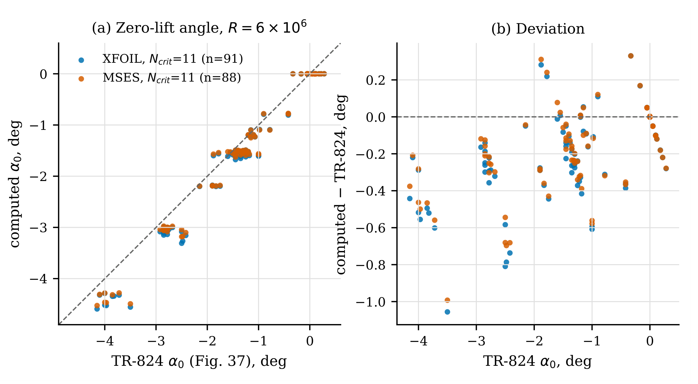
Figure 2.
Lift-curve slope against thickness ratio at , by family. Lines: faired TR-824 Figure 38 curves, smooth and with standard roughness; symbols: computed.
Figure 2.
Lift-curve slope against thickness ratio at , by family. Lines: faired TR-824 Figure 38 curves, smooth and with standard roughness; symbols: computed.
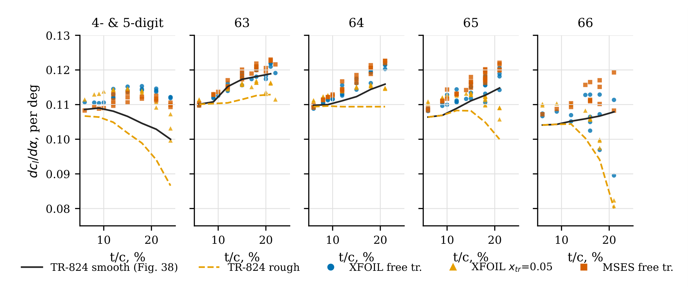
Figure 6.
Lift angle versus inverse aspect ratio: data digitised from Hoerner and Borst [5, Figure 3-2], Hoerner’s Eqs. (4), (6) and (7), and AVL 3.52 for rectangular, tapered () and elliptic planforms with section-slope factors CLAF and 1.0.
Figure 6.
Lift angle versus inverse aspect ratio: data digitised from Hoerner and Borst [5, Figure 3-2], Hoerner’s Eqs. (4), (6) and (7), and AVL 3.52 for rectangular, tapered () and elliptic planforms with section-slope factors CLAF and 1.0.
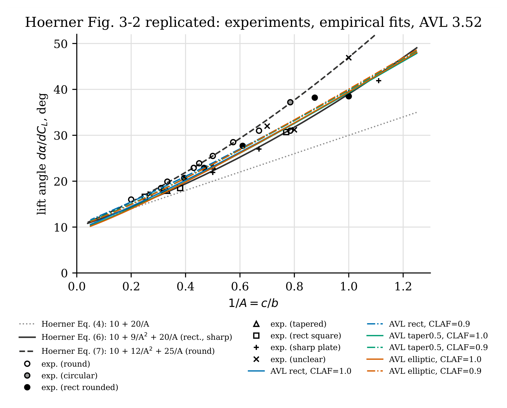
Figure 7.
Lift-curve slope versus quarter-chord sweep: data digitised from Hoerner and Borst [5, Figure 15-9], Hoerner’s Eq. (17), and AVL 3.52 for taper ratios 1.0 and 0.5. The same experimental points are shown in both panels.
Figure 7.
Lift-curve slope versus quarter-chord sweep: data digitised from Hoerner and Borst [5, Figure 15-9], Hoerner’s Eq. (17), and AVL 3.52 for taper ratios 1.0 and 0.5. The same experimental points are shown in both panels.
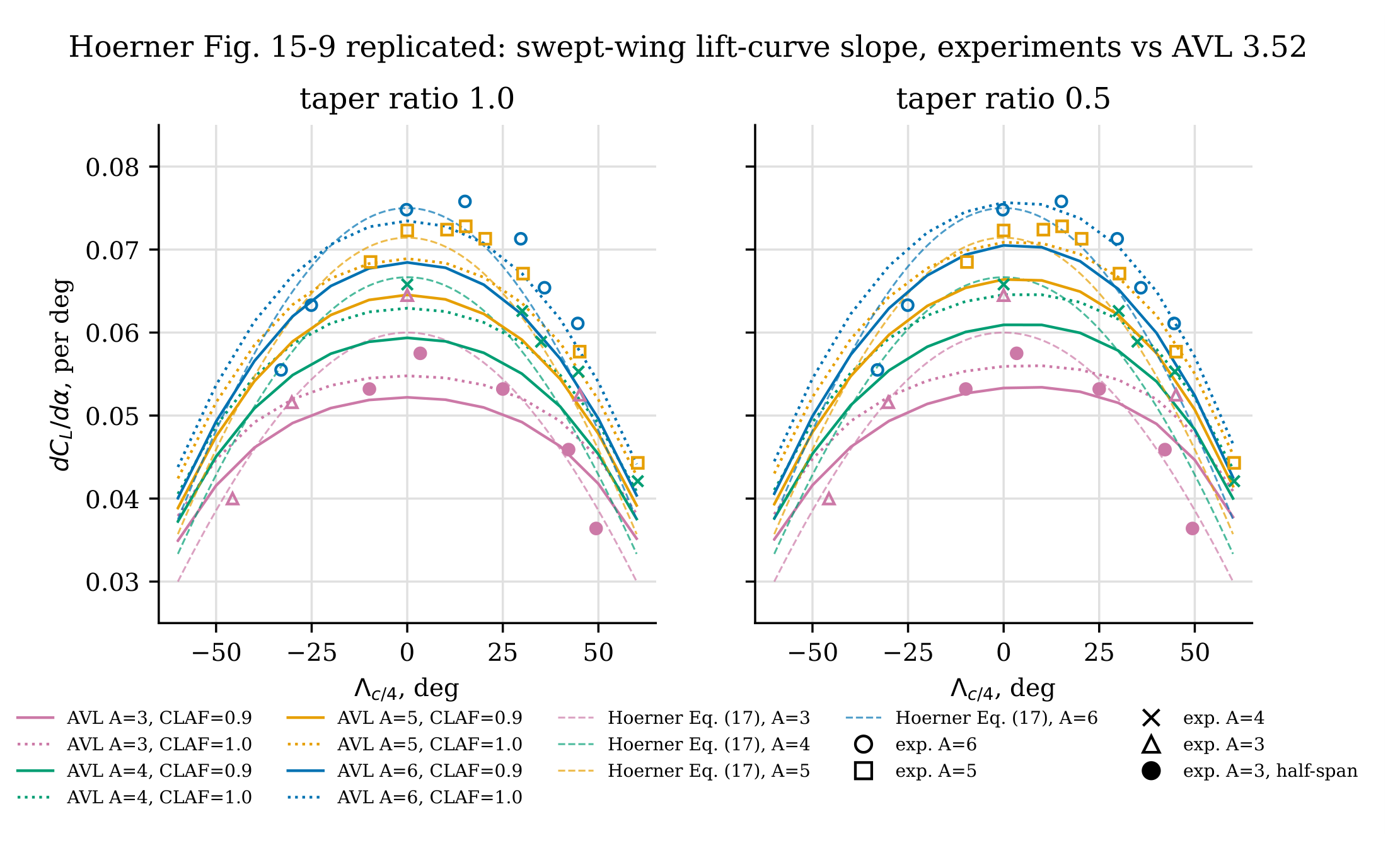
Figure 8.
Linear lift-curve slope of low-aspect-ratio wings: data digitised from Hoerner and Borst [5, Figure 17-3] (32 sharp-edged, 21 rounded-edge points), Hoerner’s Ch. XVII Eqs. (7), (9) and (10), and AVL 3.52 (CLAF ).
Figure 8.
Linear lift-curve slope of low-aspect-ratio wings: data digitised from Hoerner and Borst [5, Figure 17-3] (32 sharp-edged, 21 rounded-edge points), Hoerner’s Ch. XVII Eqs. (7), (9) and (10), and AVL 3.52 (CLAF ).
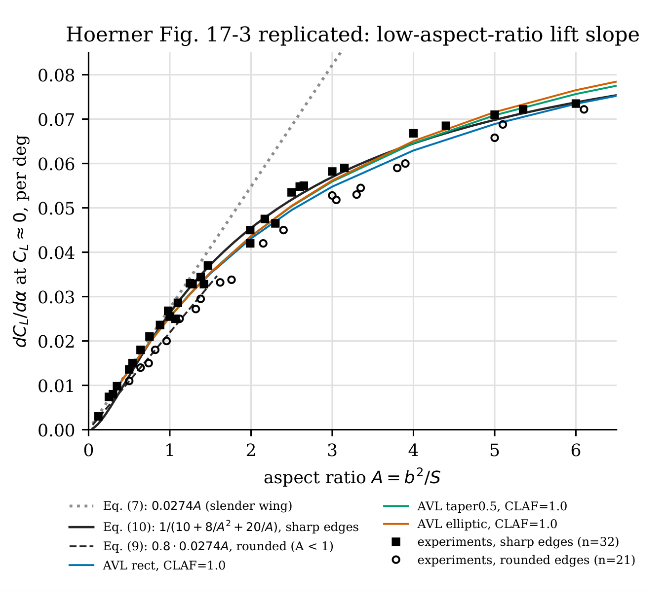
Figure 9.
Median XFOIL drag error against TR-824 (smooth, ) as a function of , per Tier-C section and over all sections.
Figure 9.
Median XFOIL drag error against TR-824 (smooth, ) as a function of , per Tier-C section and over all sections.
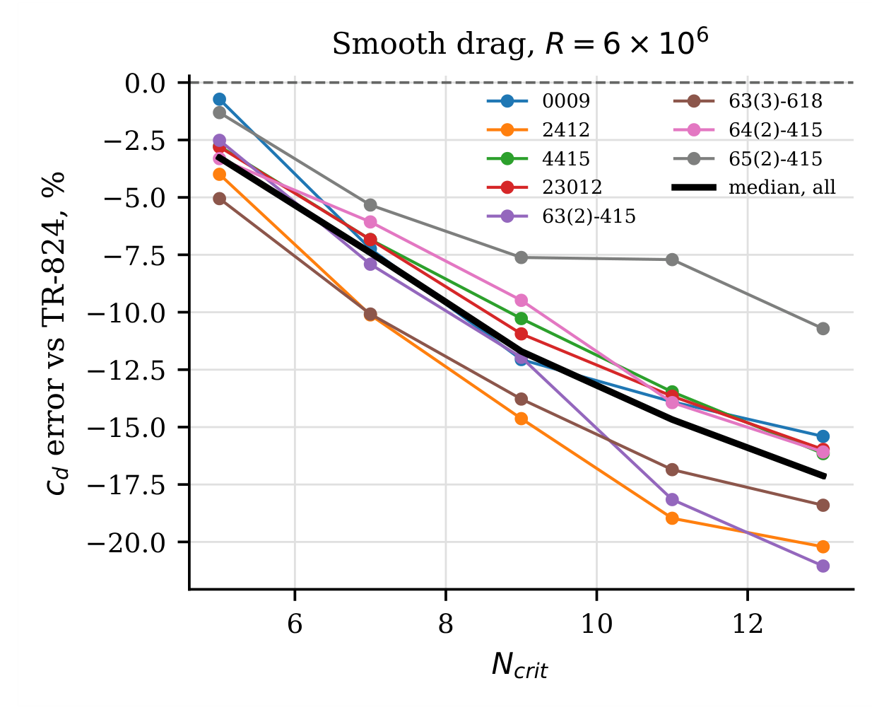
Table 1.
Scale of the automated replication.
| Item | Count |
|---|---|
| Pages text-extracted (TR-824 / Hoerner) | 261 / 507 |
| TR-824 chart pages indexed / overlaid | 128 / 112 |
| Chart legends transcribed (test R, aerodynamic-centre positions) | 112 |
| Ordinate rows transcribed from TR-824 tables (10 sections) | 270 |
| Digitised data points, TR-824 summary figures (Figures 37–39) | 315 |
| Digitised drag-polar points (8 sections, 4 conditions) | 296 |
| Digitised data points, Hoerner (3 figures) | 111 |
| Section geometries generated | 112 |
| XFOIL / MSES polars | 688 / 448 |
| AVL planform cases | 334 |
| Bibliography entries verified | 140 |
Disclaimer/Publisher’s Note: The statements, opinions and data contained in all publications are solely those of the individual author(s) and contributor(s) and not of MDPI and/or the editor(s). MDPI and/or the editor(s) disclaim responsibility for any injury to people or property resulting from any ideas, methods, instructions or products referred to in the content. |
© 2026 by the authors. Licensee MDPI, Basel, Switzerland. This article is an open access article distributed under the terms and conditions of the Creative Commons Attribution (CC BY) license (http://creativecommons.org/licenses/by/4.0/).
Copyright: This open access article is published under a Creative Commons CC BY 4.0 license, which permit the free download, distribution, and reuse, provided that the author and preprint are cited in any reuse.