Infraslow Activity in Hybrid Brain–Computer Interfaces: Signals, Derived Measures, and Validity Conditions for Wearable State Characterization

1. Introduction

From a theoretical scientific project, Brain-Computer Interfaces (BCIs) have become an important scientific and assistive technology, creating a direct communication link between the human brain and external devices. Clinical success has been achieved with conventional BCI paradigms that primarily leverage a single cortical modality, such as sensorimotor rhythms (SMRs), event-related potentials (ERPs, e.g., P300), or steady-state visually evoked potentials (SSVEPs), to provide basic communication and control for people who have severe motor impairments [1]. BCIs are used to find biomarkers of cognitive processes, and also estimate deviations from these normal processes [2]. However, single-paradigm BCIs are fundamentally limited by inherently low information transfer rates (ITRs), high classification error rates, and the phenomenon of “BCI inefficiency” in which a subset of users cannot reliably generate detectable cortical patterns[1,3].

To overcome these limitations, the paradigm of the Hybrid Brain-Computer Interface (hBCI) has emerged. By fusing two or more distinct signal modalities—either combining multiple cortical paradigms or pairing a central neural signal with peripheral physiological inputs—hBCIs significantly expand the command space, mitigate decoding ambiguities, and improve overall system performance and state characterization or classification accuracy [4,5,6,7]. While some studies show that unimodal (vs. multimodal / hBCI) meets or even sometimes exceeds multimodal hBCI decoding accuracy, these findings are specifically for binary state decoding rather than a state characterization per a geometry with graded onsets and offsets[8,9].

While contemporary hBCIs have favored integrating high-frequency or transient physiological signals (such as electromyography or electrocardiography), a largely unexploited reservoir of information resides at the opposite end of the biological frequency spectrum: infraslow dynamics. Operating at frequencies lower than 0.5 Hz, infraslow activity represents a fundamental, cross-system organizing principle of human physiology. In neural architectures, infraslow brain activity modulates cortical excitability and correlates directly with macro-scale behavioral states, vigilance, and cognitive performance[10,11]. Simultaneously, peripheral systems exhibit powerful infraslow oscillations and other types of activity, driven by autonomic, visceral, and vascular networks. These include gastric slow waves, vasomotor fluctuations, electrodermal activity (EDA), and systemic autonomic slow drifts [12,13].

Despite their ubiquity, these slow-acting biopotentials have historically been discarded as low-frequency noise or drift in traditional BCI pipelines. However, because infraslow rhythms provide the baseline physiological context and significantly affect the user's cognitive readiness, they hold unexploited promise for stabilizing and optimizing hBCI performance over extended periods. This review asks what can be rigorously measured once the range is admitted. We use the term “infraslow” throughout for activity below 0.5 Hz, following the convention that treats the band as everything beneath the standard clinical EEG range[10]. Readers should note that a narrower usage restricting the term to below 0.1 Hz is also common, and that the arguments here apply across the whole range rather than to any sub-band[14].

The exclusion of the infraslow band is more consequential than the loss of one rhythm. Respiration itself lies largely within the excluded range, and respiratory phase modulates alpha amplitude, perceptual sensitivity, and the aperiodic exponent, so a fast-band arousal measure computed without a respiratory channel is being examined in isolation with a known modulator thrown away [15,16,17]. The same holds for the other candidate common drivers of such measures (e.g. sudomotor activity, vascular tone, arterial CO₂, systemic circulatory transit) each of which has its characteristic timescale below 0.5 Hz. A high-pass at that frequency does not remove the influence of infraslow activity from the retained signal, it actually just removes the channels that would allow the infraslow band(s) to be estimated and controlled for. It also caps the longest analyzable scale at two seconds, which constrains any measure whose content is the distribution of structure across timescales, including aperiodic exponents and scaling estimates. Such high pass filtering also excludes phenomena that are constitutively slow and not recoverable from the envelope of any faster carrier: gastric–cortical coupling, slow cortical potentials, ictal DC shifts [10,18]. Without including this slower activity, changes in the faster bands already in use cannot be clearly attributed to changes in state rather than to changes in respiration, sudomotor activity, or vascular tone.

We use the phrase state characterization to refer to a combined set of metrics that describe a user identified state (e.g. level of arousal). This is different from state detection or classification. A state here is not a label drawn from a fixed inventory but a configuration across several physiological channels, no one of which is decisive e.g. cortical excitability, autonomic balance, vascular tone, and their relative timing. Characterizing such a configuration means describing where a recording sits within the range that individual has previously occupied, and how it is moving (drifting, holding, or transitioning) rather than assigning it to one of a predetermined set of categories. This is a weaker commitment than classification and a more tractable one, since it requires no prior claim about how many states there are or where their boundaries fall, questions on which the slow-band literature is not yet in a position to pronounce. The measures surveyed below (e.g. derived series computed from a single channel, summaries of their distribution, and estimators of the relationship between channels) are assessed on that basis.

Importantly, state characterization, while requiring weaker commitment, is picked not due to avoiding such commitment but for the flexibility to assay unique states and micro-trajectories towards health and pathology. Health and pathological states in mental (and also physical) health relate strongly with concepts such as arousal, autonomic balance, and wearable recording holds enormous potential to map out the trajectories over flexible time ranges[19]. Mapping out such trajectories is key for identifying interventions and optimal timing thereof.

The reason for admitting slow signals into the analysis is not that they are better arousal indices than the fast-band measures already being used, but that arousal is not the kind of thing a single index can capture[20]. Cortical excitability, autonomic balance, vascular tone, and neuromodulatory state are routinely collapsed into one latent variable and estimated through whichever proxy a given platform makes available e.g., alpha power, tonic skin conductance, heart rate variability, as though these were interchangeable. Not to mention, these proxies themselves (e.g. neuromodulatory state, autonomic balance) are themselves not monoliths. Sympathetic and parasympathetic indices can simultaneously co-exist or dissociate in complex ways[21]. Drowsiness and relaxed alertness converge on several conventional proxies while differing in what matters for most purposes related to measuring arousal. Hybrid systems are thus very sensible for correctly treating arousal as multidimensional.

While the exact function(s) and taxonomy of the infraslow band is an active area of research, strong foundational findings lay out their importance in the functioning of brain, body, and the connection between the two. Palva and Palva's (2012) taxonomy distinguishes three kinds of neuronal infraslow fluctuation: amplitude and firing-rate variability, slow scalp and cortical potentials, and BOLD fluctuations[14]. Others have replicated the associations between BOLD and EEG infraslow using simultaneous DC-EEG (EEG recording made with a DC amplifier) and resting-state fMRI[22,23]. FMRI-BOLD dynamics and cerebro-spinal fluid and vasculature changes are strongly related[24]. While there are clear correlations, and it appears that these infraslow rhythms modulate the BOLD signal, other factors also modulate BOLD as well[20].

The coupling between infraslow rhythms shows complex coordination between brain and body. For example, studies also show that infraslow vascular and neuronal fluctuations are coupled[25]. It is moreover clear that pupil size, heart rate variability, respiration, cerebro-spinal fluid flow, hemodynamics, BOLD signal and EEG power display a temporal relation with each other[26,27,28,29,30]. Many studies have links between these slow fluctuations and arousal, autonomic balance, and resting state networks. While the exact roles of the different brain and the non-neuronal slow fluctuations are still being explored, wearable hBCIs stand to harness these slow signals for improved state characterization, and also in aiding the understanding the roles of these slow fluctuations in health and disease.

We first ask what is in the band and which of its generators can be measured on a wearable device, distinguishing channels by generator character and by the stillness they demand. We then argue that the temporal assumptions an analysis makes attach to the series analyzed rather than to its physiological source, so a derived signal (time series produced by an analysis on a raw channel signal) must be assessed separately from the original raw signal. The remainder sets out the validity conditions, the hierarchy of signal types (based on analyses they lend themselves to), the analyses available without phase, and the acquisition requirements that determine which of the two possible approaches to analyze the infraslow band with.

This review is conceptual rather than systematic. Literature was identified through targeted searches of PubMed and Google Scholar on the physiological channels, derived measures, and estimator families discussed, supplemented by citation tracking from key sources, with no constraint on publication date. Coverage is deliberately uneven: the aim is to establish what a given class of signal permits, so a single well-characterized example is cited in preference to an exhaustive listing, and modeling work is cited where it bears on measurement validity rather than for its own sake.

2. Aperiodicity and the Problem of Band Definition in Infraslow Activity

The term "slow/infraslow oscillation" is applied, in practice, to a class of signals many of which display no spectral peak that is infraslow. This is not a terminological quibble, but a matter of the complexity of the slow band range space. An oscillation, in the sense that licenses phase-based analysis, is a process with a characteristic frequency to which the system returns after perturbation. What much of the infraslow literature describes is instead scale-free fluctuation, or intermittent excursion, or slow drift tracking an upstream state. The ‘infraslow’ range is not a uniform type of signal, and the term “oscillation” is not applying neatly to it.

The evidential situation is genuinely unsettled rather than merely under-reported. Across the literature, some studies emphasize the absence of peaks in infraslow spectra, others report prominent cortical oscillations with a clear peak near 0.1 Hz or near 0.02 Hz, and others still argue for multiple discrete infraslow oscillation bands rather than one [31,32]. In some cases, there is heterogeneity by state e.g. periodic in sleep, aperiodic in waking, and coupling between infraslow phase and faster-band amplitude does strengthen markedly in sleep[10,32]. But even a description taking into account of waking vs. sleep state is insufficient for a full depiction. Periodic and aperiodic character have been observed at different electrodes within the same waking recording, one trace approaching monochromatic oscillation while another was dominated by irregular sources[31]. Periodicity in this band is therefore not a property of the band, nor straightforwardly a property of the state. It is a local, intermittent, and condition-dependent property that must be established for the particular recording, the particular signal or measure derived from it, and the particular epoch in which a phase-based claim is to be made.

Thus "infraslow" names a frequency range, not a signal class, and the default expectation within that range should be aperiodicity with periodicity as the demonstrable exception. In conventional EEG one may reasonably assume alpha is oscillatory and ask whether it is present. At infraslow frequencies, one should not assume the signal is periodic, and if a peak is being claimed, one should provide evidence.

2.1. Whether to Subdivide, and on What Basis

There clearly are different bands within the infraslow range that represent different physiological processes. However, there are also gray areas about where the cuts should be made and on what basis. For example, EEG infraslow activity is sometimes partitioned into aperiodic sub-bands, on the model of the Berger bands inherited from fast EEG. But the Berger partition, whatever its own limitations, was originally motivated by visible rhythms with distinguishable spectral peaks. Partitioning aperiodic activity into bands is not something one can apply the same process to so easily. On a spectrum with no peaks, power varies continuously with frequency, and any boundary drawn across it is a choice of the analyst rather than a feature of the signal. Two consequences follow, and both are consequential for hybrid BCI work.

First, band power measured on an aperiodic background is substantially determined by the aperiodic exponent rather than necessarily by anything band-specific[33]. A steepening of the 1/f slope raises power in every low band and lowers it in every high one. If reported as "increased 0.01–0.02 Hz power," this could likely be a description of the exponent wearing a band label. Any claim about a specific infraslow sub-band therefore requires that the aperiodic component be estimated and separated first, and that the band-specific claim survive that separation.

Second, sub-bands of the infraslow range drawn from the literature carry the peak locations of the studies that proposed them, which, given the issues described above, are not always consistent with one another. A large share of “infraslow” findings are about fluctuations in band-limited power, a derived envelope, not about raw DC-coupled potential (raw potential recorded by a device without any HP filtering). Lecci's 0.02 Hz peak was in delta and sigma power during NREM[32]. Monto found that 0.01–0.1 Hz EEG fluctuations correlated with amplitudes in six faster bands and with detection performance during cognitive task execution[11]. A depression study filtered amplitude envelopes at 0.05–0.1 Hz [34]. These are different quantities from the DC potential Vanhatalo recorded[35], and there is no reason to expect them to share a peak location. Some of the apparent differences or even disagreement in ranges likely is related to these differences in the literature's own labeling.

It is notable that with envelope analyses, if one filters different amplitude envelopes together one can assess if they all go the same direction all the time which is suggestive of a gain artifact rather than modulation by slow fluctuation of neuronal origin. Hybrid BCI with multiple EEG and peripheral channels though could significantly aid in ruling out certain confounds/possibilities even if it does not fully narrow down the generator.

We therefore suggest that infraslow sub-band definition be approached through one of four principled routes rather than by inheritance.

Generator-anchored boundaries. Where a frequency range corresponds to a known peripheral generator, the boundary has physiological meaning independent of the EEG spectrum. The Stefanovska decomposition, separating myogenic, neurogenic, and endothelial contributions in the vascular signal, is boundary-setting of this kind, and its cutoffs are defensible because they refer to mechanisms rather than to observed peaks [12,36]. In a hybrid recording this route is available in a way it is not for EEG alone: the peripheral channels supply the partition, and the electrical channel can be interrogated at boundaries defined elsewhere.

Peak-anchored boundaries, verified per recording. Where a peak is demonstrated in the data at hand, a band may be defined around it, with its center and width reported for that recording rather than assumed from literature. This preserves the possibility of periodic analysis where periodicity is real, at the cost of bands that differ across subjects and sessions. This may only apply to some epochs of a signal, not necessarily as a whole as some signals are quasi-periodic.

No subdivision. Where neither route is available, which we expect to be the common case for waking infraslow EEG, the appropriate description is the aperiodic one: an exponent over a stated scale range, total power over the full range, and drift or changepoint structure. Reporting a single characterized aperiodic component is more informative than reporting four sub-band powers that are functions of it.

Provisional boundaries, declared as hypotheses. A fourth case arises where a range is neither anchored to a known generator nor to a peak demonstrated in the recording, but is suspected on other grounds to have distinct properties. A boundary adopted is a hypothesis about the signal rather than a description of it, and should be reported as one: state the range, state what motivates it, and carry forward none of the assumptions (periodicity, a stable center frequency, usable phase) that the motivating observation does not itself establish. Partitions of this kind should be held as revisable, which is what distinguishes a provisional boundary from an inherited one.

Whichever route is taken, the boundary and its justification should be reported alongside the result, and scale ranges should be given in seconds as well as in hertz. A cutoff at 0.02 Hz is a 50-second boundary. Stated that way, its relationship to the recording duration, to the stationarity assumption, and to the physiological process alleged to sit on either side of it becomes assessable by a reader in a way that the frequency alone does not permit.

3. Integrators and Oscillators

Slow physiological signals are produced by two broadly different kinds of system, and the difference matters more than the shared label "slow" suggests. A self-sustaining oscillator has an intrinsic frequency: energy circulates within the system, perturbation is followed by return, and the rhythm persists in the absence of periodic input. The cardiac pacemaker is the clearest instance, and gastric slow-wave generation is another. An integrator has no intrinsic frequency: its output accumulates the history of its inputs, and when the input changes the output moves to a new level and stays there rather than cycling back. We use "integrator" descriptively, a process whose output reflects accumulated input, so that its temporal character is set by a time constant rather than by a resonance, and intend no claim about the recurrent circuit mechanisms studied under that name in the neural-integrator literature[37]. The relevant precedent for the measurement claim is the intrinsic-timescale work, in which the autocorrelation window is used to characterize how long a system's influence persists without any assumption that it oscillates [38]. Skin temperature, tonic sudomotor level, arterial CO₂, and circulating cortisol all behave this way on the timescales at issue here. Cortisol is the partial case, the clearance kinetics are integrator-like, but the secretion is rhythmic[39].

That the slow end of physiology should be populated largely by integrators is partly a matter of loop timing. Sustained oscillation requires feedback whose delay bears a particular relation to the period[40]. At cardiac and respiratory timescales, neural and vascular delays are an appreciable fraction of the cycle, and feedback can arrive in time to shape the next one. At timescales of minutes, those same delays are a small fraction of the period, and feedback arriving promptly relative to a sixty-second cycle acts to set the level rather than to time the next excursion. Systems in this regime settle toward their inputs rather than circulating around a setpoint.

The two cases are endpoints of a continuum rather than a dichotomy, and the qualification is important. A heavily damped feedback loop with a long delay is not readily distinguishable, in a passive recording, from an integrator with no feedback at all. Slow systems frequently do possess restoring mechanisms, the baroreflex is the obvious case, that are simply too sluggish to generate rhythmic structure on the observed timescale. To describe such a system as an integrator is therefore a statement about its behavior over the window of observation, not a claim that no restoring force exists. Separating the two requires perturbation: a system with a restoring force returns to its prior level after a step input, and may overshoot in doing so, whereas an integrator moves to a new level and remains there. Resting spectra often cannot make this distinction. However, it is important to state the distinction to justify treating slow integrator processes as such rather than trying to fit them into an oscillator dynamic during a period of time where such oscillatory dynamics are not visible.

Between the two endpoints lies a regime the modeling literature has characterized more precisely than the measurement literature has. A system whose deterministic dynamics are damped (one that would ring briefly and settle) can still produce sustained irregular rhythmicity when noise repeatedly re-excites the decaying resonance[41]. Such quasi-cycles are distinguished from noisy limit cycles, where a genuine self-sustaining oscillator is perturbed, and from activity with no preferred frequency at all[42]. Usefully, intermittency is predicted by the mechanism rather than being evidence against rhythmicity: in this regime burst onsets and durations are themselves random variables[41].

The measurement consequence should be stated conservatively. This framework comes largely from modeling and cellular preparations, and no study has shown that a slow signal recorded at the scalp is a quasi-cycle rather than a noisy limit cycle. Both produce a broadened peak with variable cycle-to-cycle timing, and separating them may not be possible at wearable record lengths. What follows is therefore a caution rather than a classification. A broad peak with irregular intervals is not evidence that no resonance exists, and a verified peak is not evidence that a self-sustaining oscillator produced it. Both regimes license the same treatment (event-local rather than global phase) which is why the hierarchy below is organized by what a signal permits rather than by what generates it. Integrators fall to its lowest tier by construction: no resonance means no phase to estimate, and no recurrence means no events to mark.

4. Hardware Implementation: AC vs. DC and Confound Controls

The choice between AC-coupled and DC-coupled recording for slow-band hybrid measurement involves a genuine trade. DC-coupled amplifiers preserve the slow potential as a direct signal, offering potential access to cortical excitability shifts, direct phase relationships between cortical and peripheral slow potentials, and waveform properties that envelope-derived measures cannot capture. The cost is exposure to confounds e.g. postural drift, cable geometry changes, vascular shifts, and electrode-interface instabilities, that all manifest as slow voltage changes indistinguishable by frequency from genuine neural signals[10,43]. These confounds are theoretically tractable: accelerometry can index postural change, multiple sessions allow within-subject baselines, and shorter recording blocks limit drift accumulation. Whether these mitigations are sufficient in practice remains empirically unknown. For wearable systems deployed without continuous supervision, the AC-coupled envelope approach offers lower risk: the slow confounds never enter the recording, and the slow modulation of conventional rhythms, itself indexing arousal and excitability changes through shared physiological drivers, appears adequate for state characterization. DC-coupled slow-potential recording in wearable hybrid systems is worth pursuing as a separate research direction, with the explicit goal of validating the confound-management strategy and establishing whether the additional potential-level information illuminates aspects of brain-body coupling that envelopes miss. Until that work is complete, AC-coupled envelopes remain the more defensible choice for deployments requiring robustness.

Slow-band analysis places requirements on the recording configuration that do not arise for faster activity, because artifact and signal cannot be separated by waveform properties in this band. Two channels are conditions for interpreting slow-band results rather than improvements to them.

Motion sensing is the first. A three-axis accelerometer at the recording site is sufficient for the purpose, since electrode disturbance arises from translational movement, and the electrical consequence of a movement outlasts the movement itself, sometimes by tens of seconds while the electrode-skin junction re-equilibrates. Motion sensing therefore does not permit artifact to be excised, it identifies epochs whose slow content cannot be attributed, and a conservative post-motion exclusion window should be stated as an analysis parameter. Where a gyroscope is available it should be logged, since sustained postural change alters hydrostatic pressure and affects vascular channels at slow timescales, but rotation is not the principal mechanism of electrode disturbance and orientation is largely recoverable from the accelerometer during low-motion recording.

An adjacent skin-contacting electrode is the second. Sudomotor activity produces potentials in the same band and amplitude range as the target signal, and no property of the waveform distinguishes them[10,44]. Without a skin potential channel, slow excursions recorded at the scalp are not attributable to a cortical source, and claims resting on them are not supported.

Three further provisions are strongly recommended, and the cost of omitting each should be stated explicitly in any report that omits it.

Continuous or periodic impedance monitoring at each electrode allows junction changes to be observed directly, which is the most informative available signal about the recovery period following a disturbance. It is not universally available on wearable hardware, and where it is absent the post-motion exclusion window must be set conservatively rather than empirically.

Temperature measurement at the electrode site addresses a mechanism specific to this band: junction potential varies with temperature over timescales of minutes to tens of minutes, and in uncontrolled environments this variation is neither small nor predictable[10]. The sensor is inexpensive and adds one low-rate channel.

Timestamp synchronization across all channels should be verified rather than assumed. Absolute offsets of a few hundred milliseconds are immaterial at these timescales, but clock drift accumulating across a recording of thirty minutes or more will distort cross-channel timing relationships in precisely the range of interest, and multi-device configurations are particularly exposed[45]. Synchronization should be checked against a common reference at the start and end of each session, and the residual drift reported.

5. An Admissibility Hierarchy for Slow-Band Analysis

Analyses of infraslow signals differ not primarily in sophistication but in what they assume about the signal's temporal organization. Those assumptions are rarely stated, and are often inherited from the fast-band literature where they are usually satisfied. At infraslow ranges, they frequently are not. We therefore organize the available analyses into three tiers, ordered by the strength of the temporal assumption each requires. The ordering is a licensing hierarchy: an analysis at a given tier is admissible only if the signal satisfies that tier's assumption, and the burden is on the analyst to demonstrate this rather than presume it. Descending a tier costs specificity but never costs validity, ascending one without justification costs validity while appearing to gain specificity. The hierarchy presupposes that the series entering it has survived the confound controls set out above. Tier assignment governs which temporal assumptions a series supports, not whether its slow content is attributable to the generator of interest. A signal whose slow excursions cannot be distinguished from motion or sudomotor contamination is not a Tier 3 signal but an uninterpretable one, and Tier 3 measures computed on it describe the artifact as faithfully as they would describe physiology.

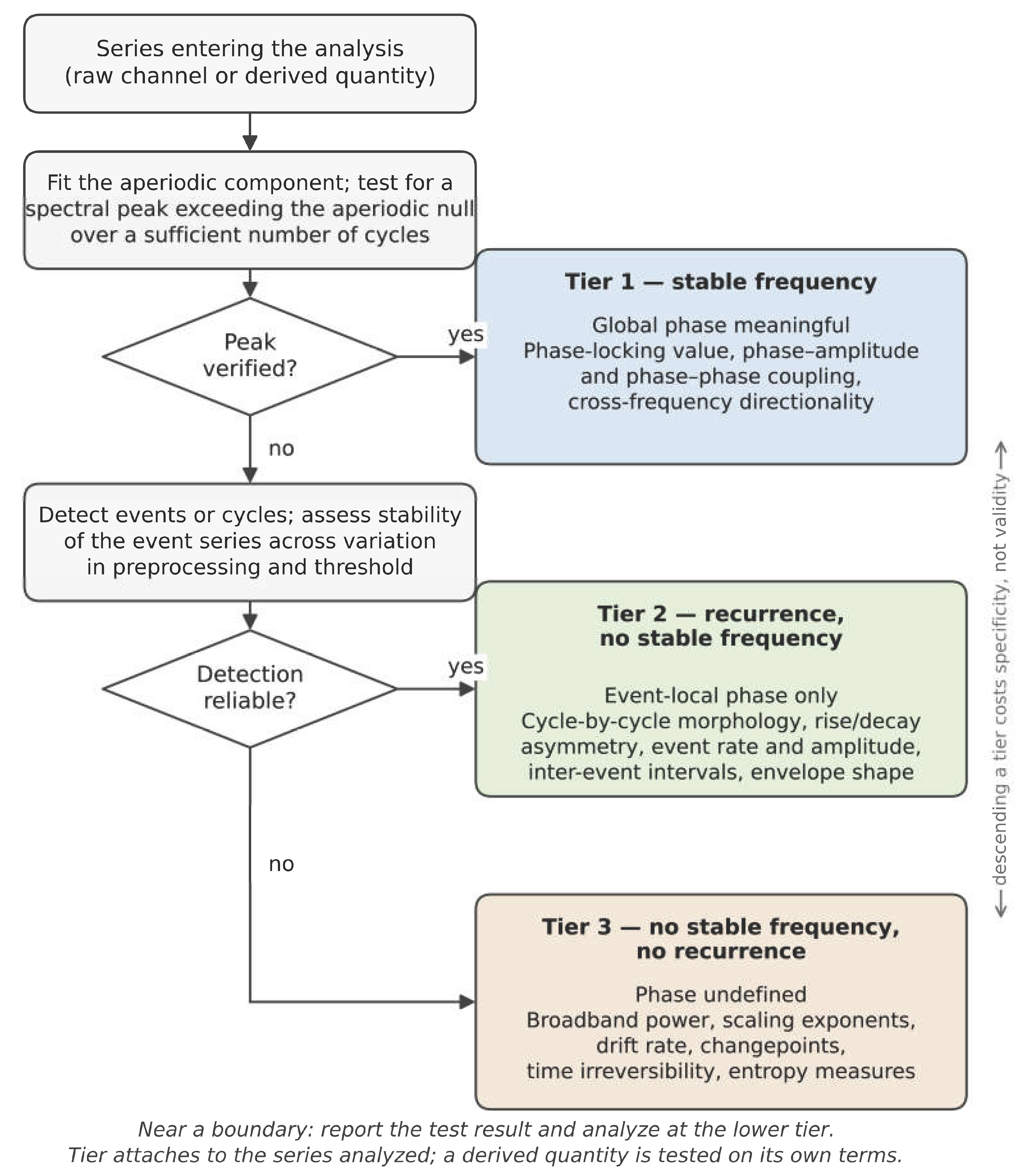
Tier 1 assumes a stable characteristic frequency, that the signal oscillates at a rate consistent enough for a phase angle to carry the same meaning at minute ten as at minute one. This licenses the full phase apparatus: phase-locking value, phase-amplitude coupling, cross-frequency directionality. It is the most informative tier and the least often warranted at infraslow frequencies. The prerequisite is a demonstrated spectral peak, not a band label. Filtering an aperiodic signal into a band and taking the analytic phase will return numbers regardless, but those numbers are properties of the filter rather than of the physiology [46]. A second prerequisite is easily overlooked: analytic phase advances nonuniformly through a non-sinusoidal cycle, so a stable frequency alone does not license phase-based coupling estimates[47]. Where the waveform is markedly asymmetric, as the gastric slow wave is, phase must either be defined cycle-by-cycle from detected waveform features or the resulting coupling estimate must be treated as potentially an artifact of waveform shape[48].

Tier 2 assumes recurrence without stable frequency, discrete events or cycles that can be individually detected, occurring at intervals that vary. Most slow physiology sits here. Phase remains meaningful but only within each detected event: one may ask where in a given burst the peak falls, or whether rise and decay are asymmetric. What is not permitted is treating that phase as a global quantity, since each event carries its own zero point and averaging angles across events with differing durations mixes reference frames. The methods native to this tier are cycle-by-cycle morphology, event statistics, and envelope structure[49].

Tier 3 assumes neither recurrence nor frequency. The signal is drift-dominated, aperiodic, or too sparse in events for reliable detection. Only magnitude and scale-structure statements survive: broadband power, scaling exponents, drift rate, changepoint structure, time irreversibility. These are the coarsest measures available and also the most robust, and for infraslow EEG in awake, seated recording they are frequently the only admissible ones.

Three qualifications govern how a tier is assigned. First, tier is a property of a recording rather than of a channel. The same signal occupies different tiers in different states: infraslow EEG is drift-dominated in awake recording but has demonstrated periodicity in postanoxic coma and in NREM sleep[50]. Respiration is event-based when spontaneous and approaches stable frequency when paced. The gastric slow wave is regular in normogastria and not during dysrhythmia[48]. Tier assignments given for particular channels in this review should therefore be read as typical for awake ambulatory recording, not as fixed attributes, and a channel found to satisfy a higher tier's assumption in a given recording may be analyzed accordingly.

Second, tier attaches to the series entering the analysis, which is usually a derived one. Raw electrocardiogram and an interbeat-interval series derived from it are different objects with different temporal organization, and as the following section develops, detection-based derivations frequently move a channel upward by converting continuous variation into locatable events. It is the derived series whose assumptions must be checked.

Third, the two criteria distinguishing the tiers, stable frequency and reliable event detection, are stated as binary but rest on continuous properties, and no threshold on either will be defensible in general. What can be specified is the test rather than the cut point. Stable frequency should be established by a spectral peak exceeding a null (null hypothesis) derived from an aperiodic fit, over a record containing enough cycles for the peak to be estimable. Reliable detection should be established by stability of event onsets and event count across a stated range of preprocessing and threshold settings, since a landmark that moves when the smoothing window changes is a property of the pipeline. The result should be reported across the range rather than reduced to a pass/fail. Instability under such variation has two possible sources, a pipeline artifact or events near the noise floor, and the two are partly separable: an event count that changes monotonically with the smoothing window points to the pipeline, whereas a stable core of onsets with marginal events entering and leaving the set points to detection sensitivity. The sensitivity of both the count and the onset locations to each perturbed parameter should therefore be reported across the range examined. Where a signal sits near a tier boundary, the appropriate response is to report the test result and analyze at the lower tier, which costs specificity and preserves validity.

Figure 1. Decision procedure for assigning an analysis tier to an infraslow series. Each gate is a test applied to the particular recording and to the series actually entering the analysis, not to a band label or a source channel. Tiers are ordered by the strength of the temporal assumption each requires. Descending a tier reduces specificity but preserves validity. Artifact rejection and confound attribution precede this procedure. The tiers govern which temporal assumptions a series supports, not whether its slow content is of physiological origin.

Figure 1. Decision procedure for assigning an analysis tier to an infraslow series. Each gate is a test applied to the particular recording and to the series actually entering the analysis, not to a band label or a source channel. Tiers are ordered by the strength of the temporal assumption each requires. Descending a tier reduces specificity but preserves validity. Artifact rejection and confound attribution precede this procedure. The tiers govern which temporal assumptions a series supports, not whether its slow content is of physiological origin.

6. Landmarks, Event Structure, and the Limits of Classification

The distinctions that follow do not change tier assignment (every signal discussed here is Tier 2) but they determine how much weight an event count can bear, and each carries its own reporting requirement.

Tier 2 admits signals that recur without a stable frequency, and licenses event-local analysis on the basis of identifiable landmarks. The signals it admits are not homogeneous, and the first distinction concerns where the landmark comes from.

In some signals the landmark is intrinsic: the waveform itself marks the event, as a discrete departure from a baseline the signal otherwise occupies. Electrodermal responses are the clearest instance, where identifying an onset requires only a threshold on rate of change[44]. Intervals between such events carry no expectation of recurrence, and a five-second interval and a four-minute interval are equally unremarkable.

In others the landmark is imposed. There is no baseline to depart from, because the signal is continuously somewhere, and the analyst must nominate what counts as the beginning of an excursion. Each candidate definition yields a different event set. Zero crossings of the demeaned signal depend on where the mean is placed, which for a drifting slow signal varies with segment length. Turning points depend on smoothing, and slow signals contain small reversals that light smoothing retains and heavier smoothing removes. Amplitude thresholds depend on the scale against which amplitude is expressed.

Imposed-landmark signals vary along three axes, which are independent of one another and each carry a distinct reporting requirement.

The first is interval regularity. Intervals may cluster tightly around a central tendency or vary over a wide range, and the interval distribution should be reported with a measure of its dispersion rather than a mean alone.

The second is whether recurrence is superimposed on independent background activity in the same frequency range. Where it is, separating excursion from background is not a preprocessing step preceding detection but a constituent of the excursion definition itself, and the choice of detrending or demeaning determines the event set. The background handling must therefore be reported alongside the detection criterion, and the two assessed together.

The third is whether recurrence is continuous or intermittent. A process may recur throughout a recording, or oscillate for a period, drift without recurring, and resume. Where intermittency is claimed, episode durations should be reported rather than assumed.

The second and third axes are difficult to separate empirically, and conflating them is a substantive risk. Weak recurrence superimposed on strong background drift will present as intermittent under a fixed detection threshold, because excursions will be detected only during periods in which the background does not obscure them. An apparent episode structure may therefore be a property of the interaction between a fixed threshold and a varying background rather than of the underlying process. Distinguishing the two requires the detection threshold to be expressed relative to local background amplitude, and the resulting episode structure to be compared against that obtained with a fixed threshold.

None of these axes affects tier assignment. All three describe signals without stable frequency whose landmarks are imposed, and all three license event-local analysis under the same conditions.

The interval distribution is computed in every case, and is standard practice for electrodermal activity. Its inferential role differs. For a candidate oscillation, the dispersion of the distribution bears on admissibility: narrow intervals support periodicity and warrant reconsidering the Tier 1 gate, while wide intervals are positive evidence that a phase-based treatment would misrepresent the signal. For an intrinsic-landmark process, the same dispersion describes the arrival pattern and is evidence against nothing.

Intermediate cases are common and should not be forced. A signal with sparse large excursions superimposed on continuous low-amplitude drift is genuinely between the available descriptions, and a clustered point process may be indistinguishable from sparsely recurrent activity at the record lengths available in wearable settings. We recommend reporting the measures that do not depend on the classification (excursion count and rate, amplitude distribution, interval distribution, and the within-excursion and sequence measures described above) and treating the classification as a stated interpretation rather than an established property. These measures are informative whichever description is correct, and they constitute the evidence by which the classification will eventually be settled.

The same reasoning governs how tier membership is assigned across a recording, given the third axis. The durations over which apparent periodicity persists in infraslow ranges have not been characterized. Two designs are available. The recording may be assigned to the lowest tier that any contributing segment supports, which is conservative and discards information. Alternatively, segments may be classified individually, with phase-based claims drawing only on segments that pass the periodicity tests.

The second design requires care. Segments selected for showing a spectral peak support claims about what occurs during periodic episodes. They do not support the claim that periodic episodes exist, since a proportion of segments drawn from an aperiodic signal will show apparent peaks by chance, particularly at the frequency resolutions available in short records. That claim requires the proportion of passing segments to be compared against the proportion obtained from aperiodic surrogates, and we recommend reporting the passing fraction with that comparison whenever segment-wise classification is used[51]. The computational cost is modest: the null distribution of passing proportions can be estimated from a limited number of surrogate realizations, since the quantity tested is a proportion across segments rather than a per-segment significance value.

Segment length is a free parameter and is not neutral. Short segments contain too few cycles to test periodicity. Long segments pool periodic and aperiodic stretches and attenuate the structure being tested. Because the episode durations that would constrain the choice are unknown, we recommend reporting the passing fraction across a range of segment lengths. A fraction stable across lengths indicates a robust result, and a fraction peaking at a particular length provides an estimate of episode duration, which is at present an open empirical question.

Table 1. Admissibility hierarchy for infraslow activity. Tier is a property of the series analyzed, established by test for a given recording.

	Tier 1	Tier 2	Tier 3
Assumption	Stable characteristic frequency	Recurrence without stable frequency	Neither
Prerequisite to demonstrate	Verified spectral peak; sufficient cycle count	Reliable event/cycle detection	None regarding temporal structure; scale range and record length must be stated
How established	Spectral peak exceeding a null hypothesis derived from an aperiodic fit, over enough cycles to estimate it	Stability of event onsets and event count across a stated range of preprocessing and threshold settings, reported across the range rather than reduced to a pass/fail	—
Phase status	Global phase meaningful	Event-local phase only	Undefined
Admissible analyses	Phase-locking value, phase-amplitude coupling, phase-phase coupling, cross-frequency directionality	Cycle-by-cycle morphology, rise/decay asymmetry, event rate and amplitude statistics, inter-event intervals, envelope shape	Broadband power, detrended fluctuation analysis and multifractal exponents, drift rate, changepoints, time irreversibility, entropy measures
Data cost	High — many cycles at a stable rate	Moderate — tens of events	Low for drift and power; scale-structure and entropy measures require long stationary windows
Failure mode if misapplied	Filter-generated phase mistaken for physiology; spurious coupling from shared arousal drive	Averaging event-local phases across variable-rate events; treating detection instability as evidence against real events	Attributing shared-driver covariance to a specific generator

Table 1. Admissibility hierarchy for infraslow activity. Tier is a property of the series analyzed, established by test for a given recording.

	Tier 1	Tier 2	Tier 3
Assumption	Stable characteristic frequency	Recurrence without stable frequency	Neither
Prerequisite to demonstrate	Verified spectral peak; sufficient cycle count	Reliable event/cycle detection	None regarding temporal structure; scale range and record length must be stated
How established	Spectral peak exceeding a null hypothesis derived from an aperiodic fit, over enough cycles to estimate it	Stability of event onsets and event count across a stated range of preprocessing and threshold settings, reported across the range rather than reduced to a pass/fail	—
Phase status	Global phase meaningful	Event-local phase only	Undefined
Admissible analyses	Phase-locking value, phase-amplitude coupling, phase-phase coupling, cross-frequency directionality	Cycle-by-cycle morphology, rise/decay asymmetry, event rate and amplitude statistics, inter-event intervals, envelope shape	Broadband power, detrended fluctuation analysis and multifractal exponents, drift rate, changepoints, time irreversibility, entropy measures
Data cost	High — many cycles at a stable rate	Moderate — tens of events	Low for drift and power; scale-structure and entropy measures require long stationary windows
Failure mode if misapplied	Filter-generated phase mistaken for physiology; spurious coupling from shared arousal drive	Averaging event-local phases across variable-rate events; treating detection instability as evidence against real events	Attributing shared-driver covariance to a specific generator

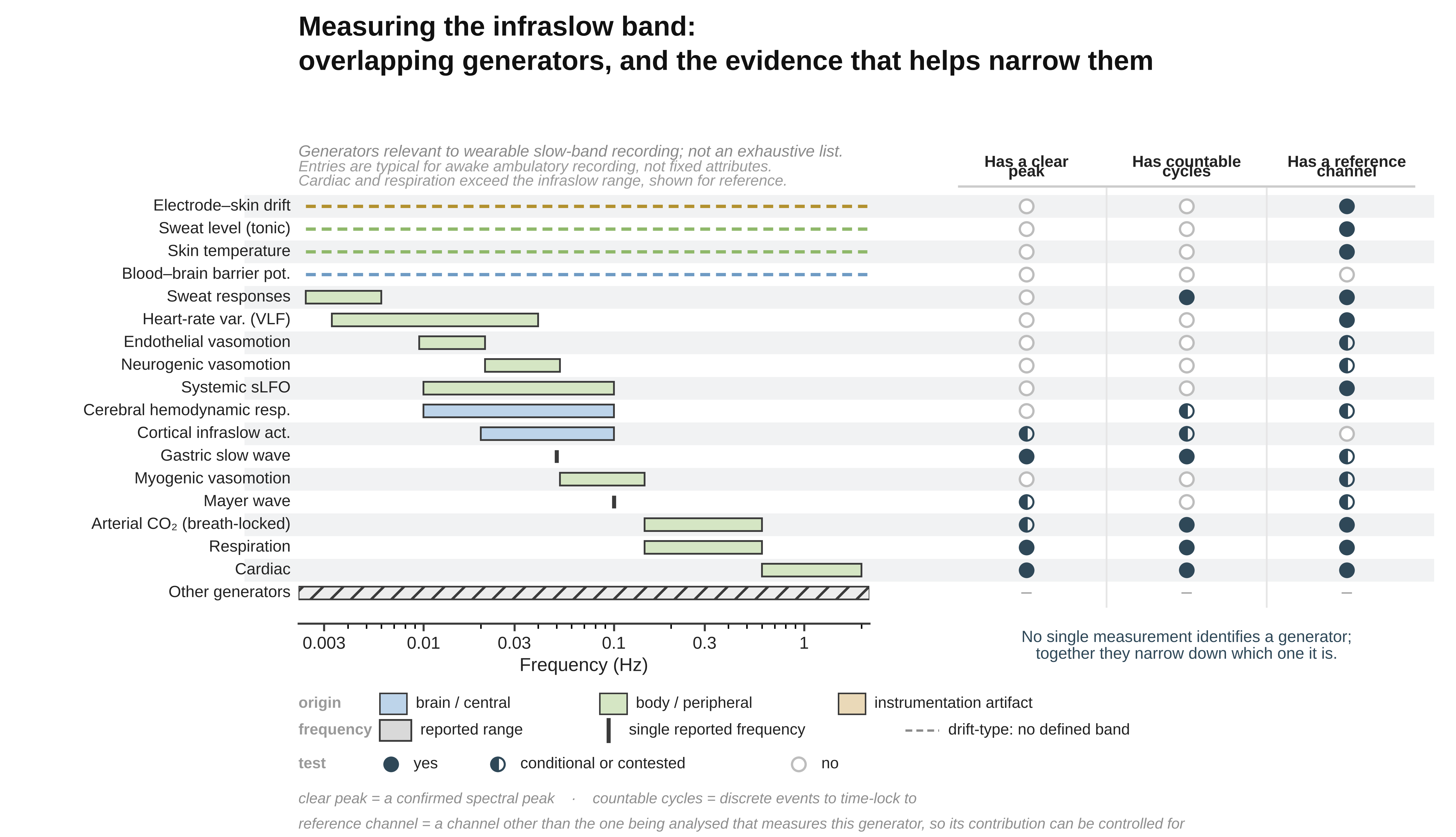
Table 2. Candidate slow channels: generator character and analysis tier. Tiers are typical for awake ambulatory recording, not fixed attributes.

Rhythm / quantity	Generator class	Characteristic band	Cycle landmarks available?	Tier
Cardiac	Pacemaker (SA node)	0.6–2 Hz	Yes	1
Respiration[15]	Central pattern generator	0.145–0.6 Hz	Yes	1–2
Gastric slow wave[48]	Pacemaker (interstitial cells of Cajal)	~0.05 Hz	Yes	1
Mayer wave[52]	Baroreflex-coupled; origin contested	~0.1 Hz	No	2–3
Myogenic vasomotion[12]	Smooth-muscle intrinsic, intermittent	0.052–0.145 Hz	No	2–3
Neurogenic vasomotion[12]	Sympathetic, intermittent	0.021–0.052 Hz	No	3
Endothelial vasomotion[12]	Intermittent, locally driven	0.0095–0.021 Hz	No	3
Cerebral hemodynamic response[25]	Driven (neurovascular coupling)	0.01–0.1 Hz	Event-locked if task-evoked	2–3
Systemic sLFO[53]	Driven (circulatory transit)	0.01–0.1 Hz	No	3
Phasic sudomotor (SCR)[44]	Event-driven, asymmetric	Events; density envelope to ~0.006 Hz	Yes (event onsets)	2
Tonic sudomotor (SCL)[44]	Drift-dominated	—	No	3
Skin temperature	Drift-dominated	—	No	3
Pupillary[54]	Events on slow drift	Events + <0.1 Hz drift	Yes (response onsets)	2
VLF HRV[55]	Derived band; contested origin	0.0033–0.04 Hz	No	3
Arterial CO₂[56]	Driven (respiratory + metabolic)	Breath-locked + slower metabolic	Yes (breath-locked component)	1–2
Blood–brain barrier potential[43]	Driven (barrier transport)	Slow drift	No	3
Electrode–skin interface drift[10]	Drift-dominated (non-physiological)	—	No	3

Cardiac and respiration exceed infraslow and are included as sources of derived slow quantities and as measured regressors for common-driver control, not as slow-band signals in their own right. The table lists generators relevant to wearable slow-band recording rather than the full space of candidates. Many further generators occupy this range without being listed, among them intracranial pressure B-waves [57], the low-frequency component of skin sympathetic outflow [58], and the thermoregulatory and hormonal mechanisms proposed for the very-low-frequency band [59].

Table 2. Candidate slow channels: generator character and analysis tier. Tiers are typical for awake ambulatory recording, not fixed attributes.

Rhythm / quantity	Generator class	Characteristic band	Cycle landmarks available?	Tier
Cardiac	Pacemaker (SA node)	0.6–2 Hz	Yes	1
Respiration[15]	Central pattern generator	0.145–0.6 Hz	Yes	1–2
Gastric slow wave[48]	Pacemaker (interstitial cells of Cajal)	~0.05 Hz	Yes	1
Mayer wave[52]	Baroreflex-coupled; origin contested	~0.1 Hz	No	2–3
Myogenic vasomotion[12]	Smooth-muscle intrinsic, intermittent	0.052–0.145 Hz	No	2–3
Neurogenic vasomotion[12]	Sympathetic, intermittent	0.021–0.052 Hz	No	3
Endothelial vasomotion[12]	Intermittent, locally driven	0.0095–0.021 Hz	No	3
Cerebral hemodynamic response[25]	Driven (neurovascular coupling)	0.01–0.1 Hz	Event-locked if task-evoked	2–3
Systemic sLFO[53]	Driven (circulatory transit)	0.01–0.1 Hz	No	3
Phasic sudomotor (SCR)[44]	Event-driven, asymmetric	Events; density envelope to ~0.006 Hz	Yes (event onsets)	2
Tonic sudomotor (SCL)[44]	Drift-dominated	—	No	3
Skin temperature	Drift-dominated	—	No	3
Pupillary[54]	Events on slow drift	Events + <0.1 Hz drift	Yes (response onsets)	2
VLF HRV[55]	Derived band; contested origin	0.0033–0.04 Hz	No	3
Arterial CO₂[56]	Driven (respiratory + metabolic)	Breath-locked + slower metabolic	Yes (breath-locked component)	1–2
Blood–brain barrier potential[43]	Driven (barrier transport)	Slow drift	No	3
Electrode–skin interface drift[10]	Drift-dominated (non-physiological)	—	No	3

Cardiac and respiration exceed infraslow and are included as sources of derived slow quantities and as measured regressors for common-driver control, not as slow-band signals in their own right. The table lists generators relevant to wearable slow-band recording rather than the full space of candidates. Many further generators occupy this range without being listed, among them intracranial pressure B-waves [57], the low-frequency component of skin sympathetic outflow [58], and the thermoregulatory and hormonal mechanisms proposed for the very-low-frequency band [59].

Table 3. Infraslow EEG sub-bands: evidential status and tier.

Sub-band	Character	Evidential status	Landmarks	Tier
~0.1 Hz[31]	Peak reported at some electrodes	Contested; collides with myogenic/Mayer band	Conditional on verified peak	1–2
0.02–0.1 Hz[35]	Best-characterized ISO range; couples to delta, sigma, alpha	Strongest evidence base	Conditional	1–2
~0.02 Hz[32]	Discrete peak reported; LC–NA linked	Sleep-dominant	Conditional	2
0.0095–0.02 Hz	Sparse; overlaps endothelial band	Weak	No	3
<0.0095 Hz	Predominantly arrhythmic	None	No	3
Aperiodic component[33]	Scale-free	Present throughout; not a band	No	3

Table 3. Infraslow EEG sub-bands: evidential status and tier.

Sub-band	Character	Evidential status	Landmarks	Tier
~0.1 Hz[31]	Peak reported at some electrodes	Contested; collides with myogenic/Mayer band	Conditional on verified peak	1–2
0.02–0.1 Hz[35]	Best-characterized ISO range; couples to delta, sigma, alpha	Strongest evidence base	Conditional	1–2
~0.02 Hz[32]	Discrete peak reported; LC–NA linked	Sleep-dominant	Conditional	2
0.0095–0.02 Hz	Sparse; overlaps endothelial band	Weak	No	3
<0.0095 Hz	Predominantly arrhythmic	None	No	3
Aperiodic component[33]	Scale-free	Present throughout; not a band	No	3

Wearability varies independently of tier, and the constraint that matters most is not sensor size but the stillness a measurement demands. Electrodermal activity, skin temperature, photoplethysmography, and respiration are measurable from wrist, finger, or chest with no postural requirement, and are the channels on which continuous ambulatory slow-band measurement realistically rests. Functional near-infrared spectroscopy is compact and can be worn with moderate movement tolerance. Pupillometry requires head-mounted optics and tolerates movement poorly, restricting it to seated or supine segments. Scalp DC-coupled EEG is more restrictive still, since the slow potentials it targets are of the same order as motion and electrode-drift artifacts. Gastric electrical activity, though generated by a genuine pacemaker at an attractive frequency, requires an abdominal montage that most wearable form factors exclude, and cerebrospinal fluid flow is not accessible outside the scanner at all. The practical consequence is that the channels best suited to unsupervised recording are largely Tier 3, while the channels that would license phase-based analysis are those that demand the most controlled conditions.

7. Derived Measures and the Tier of the Quantity Analyzed

A recorded channel and a quantity computed from it are separate objects, and the admissibility hierarchy applies to the quantity actually analyzed rather than to its source. The two frequently sit at different tiers, almost always in the same direction. Very-low-frequency HRV is derived from a channel with an intrinsic pacemaker, unambiguous cycle landmarks, and trivially wearable instrumentation, none of which transfers: the R-peaks are landmarks for the cardiac cycle, not for its modulation, and the derived band has neither landmarks nor a demonstrated peak. The Task Force standards concluded on this basis that VLF from records of five minutes or less should be avoided in interpretation, its dominant constituent being a non-harmonic component sensitive to the trend-removal algorithm applied[55]. The convenience of the source is not a discount on the cost of the derived measure, a point easily lost in wearable work, where the source channel is cheap and continuously available. The same holds above infraslow, which shows the principle concerns derivation rather than slowness. Alpha with a clear occipital peak is Tier 1, its amplitude envelope is a new time series that waxes and wanes with state on timescales that need not recur, and is commonly Tier 3[60].

Direction of movement is set by what the derivation does to landmarks. Filtering, windowing, and spectral decomposition destroy them, and the burden of demonstrating periodicity resets. Event detection can preserve or create them: the burst-density envelope of skin conductance responses is an infraslow quantity that retains individual response onsets and so remains at Tier 2. Every derived measure should therefore be reported with its timescale in seconds and its tier justified on its own terms, and where a derivation is landmark-preserving this should be stated, since it is what licenses event-based analysis at the derived timescale.

8. Individual Referencing

When doing wearable state characterization of physiology, using individual referencing as opposed to established normative databases is in many ways the only option. No normative reference exists for infraslow measures. Commercial QEEG databases high-pass at 0.5 or 1 Hz, so the band is absent from them entirely, and this holds equally for band-limited slow power, waveform-morphological quantities, and scale-structure measures such as scaling exponents or irreversibility indices. Different processing and comparison obstacles exist for each of these. Quantities expressed in microvolts depend on the reference, the electrode and gel chemistry, and the amplifier's measured low-frequency cutoff, so norms for them would have to be conditioned on a non-standardized set of acquisition steps/choices. Dimensionless quantities (scaling exponents, variability coefficients, ratios formed within a single channel) are less exposed to gain and electrode details, though still sensitive to the low-frequency response and to record length, and are correspondingly the more tractable class should such databases be assembled.

In the absence of population norms, the reference must be the individual's own accumulated distribution[61]. We suggest it be established over a fixed enrollment period defined in sessions not just minutes, since what such a period samples is contexts (times of day, task loads, sleep histories, postures) rather than duration, and that it be expressed as a distribution against which a given recording occupies a quantile, rather than as a mean from which deviation is measured. Whether the reference is then updated is a design decision with consequences: an adaptive reference will absorb any change slower than its own update interval, so if updating is permitted its timescale must be stated and must exceed the timescale of the states being characterized. Re-enrollment should be required after any change of montage, electrode type, or amplifier, since slow-band absolute values are not portable across acquisition chains. Whether a reference so constructed is stable enough to support inference is an empirical question that has not been tested for measures in this band, and we present the scheme as a proposal requiring validation rather than as established practice.

9. Families of Derived Measure Likely to Earn Their Place

Four families cover most of what a hybrid slow-band study will want, and they are worth distinguishing because they fail in different ways. The families cut across the tiers rather than mapping onto them: each is computable on most channels, and the tier determines which are licensed and how their output may be interpreted.

Event and interval series. Detection-based derivations (R-peak and interbeat-interval series, breath onsets, skin conductance response events, pupillary response onsets) convert a continuous trace into a sequence of timed events. These are the most valuable derivations available at infraslow ranges precisely because they are landmark-preserving: they license event-triggered and cycle-by-cycle analyses at timescales where nothing else does. Their cost is detection quality, and detection thresholds should be reported as analysis parameters rather than buried in preprocessing, since event rate is the quantity most sensitive to them. The derivations listed above all rest on intrinsic landmarks, where the waveform marks the event. Where events must instead be imposed on a continuously varying signal, detection additionally requires an excursion definition and a stated treatment of background activity at overlapping timescales. Where feature and background occupy the same range, the threshold determines how many events are found, so the criterion, the background handling, and the sensitivity of the event count and the onset locations to both should be reported together, the conditions under which such event series are admissible are set out above.

Envelope and density measures. Band-limited amplitude envelopes, burst-density envelopes, and tonic-level traces describe magnitude as it unfolds. They are cheap, robust, and applicable to every channel in the table, and they are the workhorse of Tier 3 analysis. Two cautions attach. Envelope extraction requires a smoothing window whose length sets the timescale of the resulting series and should be stated in seconds. And event amplitude must be normalized by prevailing tonic level before any claim that responses have grown larger rather than merely more frequent, recruitment and gain are separable, but only by a design that separates them.

Scale-structure measures. Scaling exponents, aperiodic exponents fitted to the spectrum, multifractal spectrum width, and multiscale entropy describe how structure is distributed across timescales without requiring a peak at any of them. They are the natural description of an integrator and the most defensible summary of an aperiodic slow channel. All of them are defined relative to a scale range and a detrending order, and all are inflated or distorted by unremoved trend. On channels that have not equilibrated (which is most slow channels in the first five to ten minutes) the reported exponent is a statement about the drift [62]. A further caution applies where recurrence is intermittent: an exponent estimated over a record containing both recurrent and quiescent periods summarizes the mixture rather than either regime, and where episode structure is suspected it should be reported alongside the proportion of the record contributing each regime, with the detection criterion that produced it, since apparent intermittency may reflect the interaction between a fixed threshold and a varying background rather than a property of the signal.

Distributional and dynamical measures. Sample and permutation entropy, Lempel–Ziv complexity, and time irreversibility characterize predictability and the arrow of time without assuming periodicity, linearity, or stationarity in the strong sense [63]. Time irreversibility deserves particular mention in this setting: it distinguishes actively driven from equilibrium dynamics, which is close to the integrator-versus-oscillator question and is one of the few ways to approach it without perturbation, and it also serves as a sequence-level descriptor of detected excursions where an event series is available [64]. Its cost is interpretive rather than computational, these measures answer real questions but map onto physiology less directly than the others, and should be reported alongside a measure whose physiological meaning is transparent.

10. Simple Measures, Sufficient Inference

The methods surveyed above are ordered by what they assume, not by sophistication, and the least demanding of them are often sufficient for the inference a hybrid BCI actually needs to make. A system designed to detect and track state transitions is not required to identify the generator of a slow fluctuation, establish its periodicity, or resolve its phase relationship to faster activity. It is required to distinguish one state from another in the same individual and to register when the transition occurs. Drift rate and direction, changepoint location, event rate and amplitude distribution, envelope smoothness, and rise-to-decay asymmetry are all defined on aperiodic, non-stationary, drift-dominated traces, and all of them can differ systematically between states. Where they do, the state is decodable, and nothing has been assumed that the signal does not supply. What the phase-based alternative would add is discussed below. What is given up by declining phase is therefore smaller than it first appears, and what is gained is that the analysis no longer fails silently when the periodicity assumption is unmet.

The simpler measures are also well matched to the referencing scheme set out above: a claim that a participant's morphology differs between their own states is a within-subject comparison, and is therefore unaffected by the montage, electrode chemistry, empirically characterized low-frequency response, and individual vascular and autonomic baseline that make between-subject norms unavailable in this band.

11. Simple Measures, Benefits for Wearable Acquisition

This choice has direct consequences for what hardware and what protocol are required. Two constraints dominate the feasibility of slow-band recording outside the laboratory: the duration of the recording and the stillness of the participant. Cycle-based analysis binds both. The convention that a record should contain roughly ten cycles of the lowest frequency of interest is a heuristic rather than a derived criterion[55]. It underlies the familiar five-minute short-term HRV standard, but no analytical justification for it appears to have been published[65], and even as a rule of thumb it places a 0.02 Hz component at roughly eight minutes and a 0.006 Hz component at nearly half an hour, before any allowance for interface equilibration. Because the estimate is of a frequency, epochs corrupted by movement cannot simply be excised without consequence: excision introduces discontinuities at the joins, and sharp deflections of this kind are an established source of spurious cross-frequency coupling[66]. Measures defined on morphology and distribution are bound differently. Event statistics accumulate across whatever epochs are clean, so corrupted segments can be rejected and the remainder pooled, subject to the sampling bias that any rejection procedure introduces, which should be reported. Drift and changepoint measures are local in time and do not require a stationary segment spanning the whole session. Scaling exponents still require the longest analyzed scale to be a small fraction of the record and so retain a duration cost, but one set by the scale range chosen rather than by the slowest component present.

The motion argument requires more care than it is usually given. It is not that slow measures are insensitive to movement, movement is among the largest contaminants of slow-band recording, and the DC-coupled potential in particular responds to any change in electrode–skin contact, scalp perfusion, or sustained muscle tension with excursions comparable to or larger than the signal. The argument is narrower: the measures differ in how well a partially corrupted record can be salvaged. A morphological or distributional estimate is computed over surviving epochs and degrades roughly in proportion to how many are lost, whereas a spectral or phase estimate is degraded both by the loss and by the discontinuities that removal creates. This distinction favors the simpler measures in any setting where artifact-free continuous recording cannot be guaranteed, which describes most wearable deployment. It does not license recording during ambulation or during speech, and it does not remove the need for an equilibration interval at the start of a session.

The band-limited envelope route inherits these advantages and adds one of its own. Because the envelope is computed from carriers well above the movement and drift bands, it is protected from the additive slow contaminants that reach the potential directly, and because it can be computed in several carrier bands simultaneously, it supplies a within-signal test: a coherent excursion across all carriers is characteristic of a gain change, whereas a band-differentiated one is not. Together these suggest a plausible minimum configuration for a wearable slow-band hybrid system, a small number of electrodes, an individual baseline recorded under controlled conditions, and subsequent recording in less controlled conditions evaluated against that baseline.

12. Coupled-Oscillator Analysis When One Limb Is Not an Oscillator

The coupled-oscillator framework is a genuine achievement of the fast-band literature and it presumes what its name says. Phase difference, phase-locking value, synchronization index, and the whole apparatus of entrainment are defined for systems that each possess a phase, an intrinsic frequency and a reproducible zero. When one limb is an integrator, these quantities can still be computed and will still return numbers, but the numbers describe the filter applied to the integrator rather than the coupling between the systems. The framework does not degrade gracefully here, it fails silently, which is worse.

We suggest the governing rule be that the admissible analysis for a coupled pair is set by the lower-tier limb. What matters is that this is a redirection rather than a loss. A Tier 3 analysis of the pair still has a full inventory available: amplitude-to-amplitude covariance and its state-dependence; lagged amplitude relations, where the lag is itself a finding and carries transmission-delay information that a phase statistic discards; event-triggered averaging of the fast channel around detected excursions in the slow one; conditional entropy or mutual information where the relationship may be nonlinear; joint state-space description of the two channels together. Where the slow limb reaches Tier 2 (a demonstrable recurring excursion, a gastric wave, an identified sudomotor burst sequence) timing can be defined relative to detected events rather than to an abstract phase, which is a real gain in specificity and is available considerably more often than Tier 1 methods are.

The temptation is to treat these as fallbacks, and it should be resisted, because the coupling question a hybrid BCI actually needs to answer is usually within their reach. Detecting that two channels covary differently in one state than another, and registering when that changes, requires no phase at all. It requires only that the association structure be measurable and that it differ between states. Phase appears to add a direction, that the slow limb governs the fast, and that appearance is what makes the alternatives look like concessions. But the non-phase measures answer the question posed above, and they work on the aperiodic, drifting, intermittent signals of the slow band.

Two constraints apply throughout. The first is identifiability: two channels driven by a common upstream state will co-vary regardless of any coupling between them, and no analysis of the two channels alone separates the cases. In a hybrid recording this is tractable in a way it is not for EEG alone, since the candidate drivers (respiration, CO₂, sudomotor activity, systemic circulation) can be measured directly and entered as regressors, which is the strongest argument for building the peripheral limb out fully rather than treating it as ancillary. The second is the choice of null: coupling should be tested against surrogates that shift one channel in time relative to the other, leaving each signal otherwise intact, rather than against phase-randomized surrogates, which discard the waveform structure these analyses depend on[51].

Phase–amplitude coupling can only express one direction: the phase of the slower signal against the amplitude of the faster[46]. The finding that slow rhythms appear to govern fast ones is therefore partly constitutive of the measure rather than discovered by it, since a symmetric analysis is rarely computed within the same formalism. How far this accounts for the observed asymmetry in the literature is not fully known.

13. Estimators for the Non-Phase Inventory

Estimators licensed at Tier 3. Amplitude covariation is the entry point, and lagged cross-correlation extends it at negligible cost[67]. Where several peripheral channels are available, a distributed lag regression (modeling the cortical measure as a function of each peripheral measure across a range of lags) generalizes this without additional machinery, yields interpretable coefficients, and admits covariates directly. It is the plainest available treatment and should be the baseline against which more elaborate estimators are judged, since an analysis that adds complexity without improving on it has not earned the complexity. Where both channels carry long-range temporal correlations, as slow physiological signals characteristically do, ordinary cross-correlation becomes unreliable: shared trend inflates the estimate and the effective number of independent samples falls well below the nominal one. Detrended cross-correlation analysis addresses this directly, asking whether two long-memory series share scaling structure across a range of timescales rather than whether their raw values track[68]. Where a scaling exponent has already been computed for each channel separately, its bivariate counterpart is a short additional step and a better-founded one.

Conditioning (regressing out a third variable possibly accounting for a correlation in two variables) is available at any tier and is the cheapest response to the identifiability problem (figuring out what drives a correlation, is it the first variable that drives the second, the second that drives the first, or alternatively a third, or fourth, or fifth, etc. variable driving the first two simultaneously). Where a candidate common driver has been measured (respiration, motion, sudomotor activity) partial correlation between the two channels of interest, controlling for that third series, distinguishes an association that survives the control from one that does not. Partial coherence and partial regression extend this to the frequency domain and to multiple simultaneous controls. None of this establishes coupling, since an unmeasured driver remains possible, but it converts a general worry into a specific and testable one at no cost beyond the peripheral channels a hybrid system already records.

Where the relationship may be nonlinear but no directional claim is intended, distance correlation is a better first move than mutual information: it requires no binning, no embedding parameters, and no long record, is zero exactly when two variables are independent including under nonlinear dependence, and admits a straightforward permutation test[69]. Mutual information answers a similar question with a richer interpretation but at substantially higher data cost, and with estimator choices (binning scheme or nearest-neighbor parameter) that materially affect the result and are seldom reported[70].

Directional inference is likewise licensed at Tier 3, which is worth stating plainly because direction is widely assumed to require phase. Granger causality asks whether one channel's past improves prediction of another's future beyond that channel's own history. It is estimable on records of moderate length and has mature bias corrections and standard inferential procedures[71]. It assumes linearity, requires stationarity or explicit differencing, and is vulnerable to unmeasured common inputs as any predictive criterion is, but for the record lengths a wearable study will realistically produce, it is the directed estimator that can actually be computed. Transfer entropy generalizes the same logic without the linearity assumption and is defined for aperiodic and non-stationary signals. Its cost is data: strongly biased at short record lengths, sensitive to embedding dimension and lag, and requiring either substantial data or explicit bias correction to be trustworthy[72]. An estimate accompanied by neither a bias correction nor a surrogate distribution should not be reported.

Estimators licensed at Tier 2. Where the slow limb supports reliable event detection, a further set opens, and it contains the most specific estimators available without a periodicity assumption. As mentioned, their specificity is contingent on the event definition holding up. A peri-event time course built around detected events (skin conductance response onsets, respiratory onsets, detected excursions in a slow channel) yields not a scalar association but a temporal profile, and the position of the cortical change relative to the event carries the interpretive weight. A cortical change preceding the peripheral event does not by itself support central drive, since a common driver reaching two effectors through pathways of different latency produces the same ordering. What matters is whether the observed lag departs from what those known latencies predict. A change following the event indicates feedback or instrumental contamination, which the cross-band consistency check distinguishes. This narrows the gap between common causation and genuine coupling empirically rather than conceding it, and it requires no Tier 1 assumption. Peri-event variance is worth computing alongside the mean, since a change in dispersion without a change in central tendency is a real and easily missed effect. Where both channels yield event series, their coincidence can be tested against a permutation null, a complete coupling test requiring nothing but two sets of timestamps[73]. Detected changepoints are themselves events in this sense, and testing whether changepoints in two channels co-occur above chance asks whether the channels transition together, a question closer to what a state-characterization system needs than any continuous coupling measure, and answerable with machinery the analysis already contains[74]. Point-process methods extend this by modeling event rate as modulated by a continuous covariate without binning, avoiding the arbitrary window length that binning imposes[75].

These event-based estimators are the practical return on the tier framework. They are more specific than anything available at Tier 3 and require no periodicity, which is why establishing whether a slow channel supports reliable event detection is worth the effort the taxonomy asks of it.

Beyond the inventory. Cross-recurrence quantification describes when two trajectories visit similar regions of their respective spaces and how long they remain there, assuming neither periodicity nor stationarity, though its sensitivity to embedding, delay, and recurrence threshold makes reported values difficult to compare unless all three are stated[76]. Beyond it lie the methods proper to a dynamical-systems treatment, delay-embedding reconstruction and convergent cross mapping, the latter offering a principled separation of coupling from common driving[77]. These presume deterministic dynamics on a low-dimensional attractor, an assumption this framework holds should be demonstrated rather than adopted. They are noted as the direction in which validated individual characterization opens rather than as present recommendations.

Cost. These estimators do not carry equal data requirements, and the gradient does not follow the tier ordering. Amplitude covariation, distributed lag regression, partial correlation, distance correlation, peri-event averaging, coincidence testing, and changepoint concordance are stable on short and fragmented records and are appropriate for ambulatory deployment. Granger causality occupies a middle position, requiring stationarity but not extensive data. Detrended cross-correlation, mutual information, transfer entropy, and cross-recurrence require long, approximately stationary windows and belong to a research layer rather than a deployed system. Tier licensing determines what may be computed. Data length determines what can be computed well, and the two constraints are independent.

14. Conclusions

Infraslow activity is measurable in a hybrid recording, and much of what makes it difficult is not intrinsic to the band but inherited: analytical conventions developed where stable oscillations could be assumed, applied where they cannot. The central claim of this review is that admissibility in this range is a property of a particular recording and a particular derived quantity, established by test, rather than a property of a frequency range or a channel. The three-tier hierarchy is a way of making that determination explicit and of keeping the analysis within what the determination licenses.

Three consequences follow. First, the burden of proof inverts at infraslow ranges. Aperiodicity is the reasonable default and periodicity the demonstrable exception, so a phase-based analysis requires positive evidence of a spectral peak in the recording at hand rather than a band label inherited from the literature. Analyses that skip this step do not fail visibly, they return well-behaved numbers describing the filter that produced them.

Second, the constraint is narrower than it appears. Declining phase does not cost the ability to detect states, register transitions, or estimate directional relationships between channels. Magnitude covariation, scale-structure measures, changepoint detection, event-locked analysis, and predictive directional estimators are all defined on aperiodic, non-stationary, intermittently corrupted signals. What phase adds is mechanistic specificity within transitions, for the reasons set out above. The measures that survive the constraint are also those that survive fragmented ambulatory recording, which is what makes wearable slow-band measurement appear realistic rather than aspirational.

Third, the two acquisition routes into this band are not variants of one method. Band-limited envelopes and DC-coupled potentials are different physical quantities with different confound structures, and the choice between them is a choice about which risks to accept. Envelopes are the more defensible default for unsupervised deployment. DC-coupled recording offers strictly more information and remains, in the wearable case, an unvalidated proposition rather than a recommended practice.

What the field lacks is not analytical technique but the empirical work that would let these recommendations be replaced by evidence: validation of individual referencing across sessions, characterization of the confound structure of ambulatory DC recording, and minimum-record-length results for the entropy, irreversibility, and changepoint measures on which so much of the tractable inventory depends. In the meantime, the requirement that costs least and returns most is reporting. Because tier assignment is established by test rather than assumed, a slow-band result is interpretable only if the reader can see which tests were passed: the empirically characterized low-frequency response of the recording chain, the scale range in seconds, the detrending order and method, the segment length, and the number of cycles or excursions the analysis rests on. Where an event definition is used, the excursion criterion and the handling of background should be stated. Where surrogates are used, their construction should be given, since surrogates that destroy timing test a different null hypothesis than those that preserve it. None of this is specific to infraslow activity, but the absence of population norms in this range makes it consequential in a way it is not at faster frequencies. That is a low bar, and the band will not become interpretable until the literature clears it.

15. Limitations

This review is a methodological argument rather than an empirical study, and its recommendations carry the status appropriate to that. None has been validated against slow-band physiological data. The tier boundaries are proposed on the basis of what each class of analysis assumes, not derived from a demonstration that analyses fail in the manner predicted when those assumptions are violated. The estimator guidance is reasoned from the statistical properties of the estimators and from simulation work conducted largely on synthetic signals, rather than benchmarked on the strongly autocorrelated, non-stationary, artifact-prone recordings that motivate it. The individual-referencing scheme is a design proposal whose central premise, that a within-subject distribution accumulated across sessions is stable enough to support inference, has not been tested for any measure in this band. Where the text recommends a practice, it recommends it as the more defensible of the available options given what is currently known, which is a weaker warrant than evidence of superiority.

Several specific gaps should be noted. The data requirements given for measures other than spectral and scaling estimates are extrapolations: the methodological literature on minimum record length is firm for cycle-based and detrended fluctuation estimates and thin for entropy, irreversibility, and changepoint measures, particularly in the low-frequency regime where the effective number of independent samples falls far below the nominal one. The confound structure of DC-coupled wearable device recording is described from known mechanisms rather than measured, and no study has systematically disentangled postural drift from neural signal in ambulatory slow-band EEG. The channel taxonomy assigns tiers typical of awake ambulatory recording, and its assignments will not hold in sleep, in pathology, or under paced protocols. Finally, this review does not address the ethical and privacy questions that continuous physiological state characterization raises, which are substantial and are treated elsewhere.

References

- Edelman, B.J.; Zhang, S.; Schalk, G.; Brunner, P.; Müller-Putz, G.; Guan, C.; He, B. Non-Invasive Brain-Computer Interfaces: State of the Art and Trends. IEEE Rev. Biomed. Eng. 2025, 18, 26–49. [Google Scholar] [CrossRef] [PubMed]
- Zander, T.O.; Kothe, C. Towards Passive Brain–Computer Interfaces: Applying Brain–Computer Interface Technology to Human–Machine Systems in General. J. Neural Eng. 2011, 8, 025005. [Google Scholar] [CrossRef] [PubMed]
- Thompson, M.C. Critiquing the Concept of BCI Illiteracy. Sci. Eng. Ethics 2019, 25, 1217–1233. [Google Scholar] [CrossRef] [PubMed]
- D’Mello, S.K.; Kory, J. A Review and Meta-Analysis of Multimodal Affect Detection Systems. ACM Comput. Surv. 2015, 47, 43:1–43:36. [Google Scholar] [CrossRef]
- Debie, E.; Fernandez Rojas, R.; Fidock, J.; Barlow, M.; Kasmarik, K.; Anavatti, S.; Garratt, M.; Abbass, H.A. Multimodal Fusion for Objective Assessment of Cognitive Workload: A Review. IEEE Trans. Cybern. 2021, 51, 1542–1555. [Google Scholar] [CrossRef] [PubMed]
- Pfurtscheller, G.; Allison, B.Z.; Bauernfeind, G.; Brunner, C.; Solis Escalante, T.; Scherer, R.; Zander, T.O.; Mueller-Putz, G.; Neuper, C.; Birbaumer, N. The Hybrid BCI. Front. Neurosci. 2010, 4, 30. [Google Scholar] [CrossRef] [PubMed]
- Hong, K.-S.; Khan, M.J. Hybrid Brain–Computer Interface Techniques for Improved Classification Accuracy and Increased Number of Commands: A Review. Front. Neurorobotics 2017, 11, 35. [Google Scholar] [CrossRef] [PubMed]
- Booth, L.; Mehmood, A.; Zeinali, M. Benchmarking Multimodal Workload Classification: Effects of Modality, Validation Protocol, and Segmentation Contrast on an Open Graded-Arithmetic Dataset. Bioengineering 2026, 13, 820. [Google Scholar] [CrossRef] [PubMed]
- Hogervorst, M.A.; Brouwer, A.-M.; van Erp, J.B.F. Combining and Comparing EEG, Peripheral Physiology and Eye-Related Measures for the Assessment of Mental Workload. Front. Neurosci. 2014, 8, 322. [Google Scholar] [CrossRef] [PubMed]
- Tallgren, P.; Vanhatalo, S.; Kaila, K.; Voipio, J. Evaluation of Commercially Available Electrodes and Gels for Recording of Slow EEG Potentials. Clin. Neurophysiol. 2005, 116, 799–806. [Google Scholar] [CrossRef] [PubMed]
- Monto, S.; Palva, S.; Voipio, J.; Palva, J.M. Very Slow EEG Fluctuations Predict the Dynamics of Stimulus Detection and Oscillation Amplitudes in Humans. J. Neurosci. 2008, 28, 8268–8272. [Google Scholar] [CrossRef] [PubMed]
- Stefanovska, A.; Lotric, M.; Kvernmo, H. Wavelet Analysis of Oscillations in the Peripheral Blood Circulation Measured by Laser Doppler Technique. IEEE Trans. Biomed. Eng. 1999, 46, 1230–1239. [Google Scholar] [CrossRef] [PubMed]
- Azzalini, D.; Rebollo, I.; Tallon-Baudry, C. Visceral Signals Shape Brain Dynamics and Cognition. Trends Cogn. Sci. 2019, 23, 488–509. [Google Scholar] [CrossRef] [PubMed]
- Palva, J.M.; Palva, S. Infra-Slow Fluctuations in Electrophysiological Recordings, Blood-Oxygenation-Level-Dependent Signals, and Psychophysical Time Series. NeuroImage 2012, 62, 2201–2211. [Google Scholar] [CrossRef] [PubMed]
- Kluger, D.S.; Gross, J. Respiration Modulates Oscillatory Neural Network Activity at Rest. PLoS Biol. 2021, 19, e3001457. [Google Scholar] [CrossRef] [PubMed]
- Kluger, D.S.; Forster, C.; Abbasi, O.; Chalas, N.; Villringer, A.; Gross, J. Modulatory Dynamics of Periodic and Aperiodic Activity in Respiration-Brain Coupling. Nat. Commun. 2023, 14, 4699. [Google Scholar] [CrossRef] [PubMed]
- Kluger, D.S.; Balestrieri, E.; Busch, N.A.; Gross, J. Respiration Aligns Perception with Neural Excitability. eLife 2021, 10, e70907. [Google Scholar] [CrossRef] [PubMed]
- Richter, C.G.; Babo-Rebelo, M.; Schwartz, D.; Tallon-Baudry, C. Phase-Amplitude Coupling at the Organism Level: The Amplitude of Spontaneous Alpha Rhythm Fluctuations Varies with the Phase of the Infra-Slow Gastric Basal Rhythm. NeuroImage 2017, 146, 951–958. [Google Scholar] [CrossRef] [PubMed]
- Jin, Y.; Yao, H. Spatiotemporal Dynamics of Brain-Heart Communication: From Asymmetric Neural Regulation to Systemic Neuro-Immune-Endocrine Interactions. Rev. Neurosci. 2026. [Google Scholar] [CrossRef] [PubMed]
- Watson, B.O. Cognitive and Physiologic Impacts of the Infraslow Oscillation. Front. Syst. Neurosci. 2018, 12, 44. [Google Scholar] [CrossRef] [PubMed]
- Berntson, G.; Cacioppo, J.; Quigley, K. Autonomic Determinism: The Modes of Autonomic Control, the Doctrine of Autonomic Space, and the Laws of Autonomic Constraint. Psychol. Rev. 1991, 98, 459–487. [Google Scholar] [CrossRef] [PubMed]
- Hiltunen, T.; Kantola, J.; Elseoud, A.A.; Lepola, P.; Suominen, K.; Starck, T.; Nikkinen, J.; Remes, J.; Tervonen, O.; Palva, S.; et al. Infra-Slow EEG Fluctuations Are Correlated with Resting-State Network Dynamics in fMRI. J. Neurosci. 2014, 34, 356–362. [Google Scholar] [CrossRef] [PubMed]
- Grooms, J.K.; Thompson, G.J.; Pan, W.-J.; Billings, J.; Schumacher, E.H.; Epstein, C.M.; Keilholz, S.D. Infraslow Electroencephalographic and Dynamic Resting State Network Activity. Brain Connect. 2017, 7, 265–280. [Google Scholar] [CrossRef] [PubMed]
- Liu, X. Decoupling Between Brain Activity and Cerebrospinal Fluid Movement in Neurological Disorders. J. Magn. Reson. Imaging 2024, 60, 1743–1752. [Google Scholar] [CrossRef] [PubMed]
- Mateo, C.; Knutsen, P.M.; Tsai, P.S.; Shih, A.Y.; Kleinfeld, D. Entrainment of Arteriole Vasomotor Fluctuations by Neural Activity Is a Basis of Blood-Oxygenation-Level-Dependent “Resting-State” Connectivity. Neuron 2017, 96, 936–948.e3. [Google Scholar] [CrossRef] [PubMed]
- Bolt, T.; Wang, S.; Nomi, J.S.; Setton, R.; Gold, B.P.; deB. Frederick, B.; Yeo, B.T.T.; Chen, J.J.; Picchioni, D.; Duyn, J.H.; et al. Autonomic Physiological Coupling of the Global fMRI Signal. Nat. Neurosci. 2025, 28, 1327–1335. [Google Scholar] [CrossRef] [PubMed]
- Gu, Y.; Sainburg, L.E.; Kuang, S.; Han, F.; Williams, J.W.; Liu, Y.; Zhang, N.; Zhang, X.; Leopold, D.A.; Liu, X. Brain Activity Fluctuations Propagate as Waves Traversing the Cortical Hierarchy. Cereb. Cortex 2021, 31, 3986–4005. [Google Scholar] [CrossRef] [PubMed]
- Yang, Y.; Leopold, D.A.; Duyn, J.H.; Liu, X. Sensory Encoding and Memory Retrieval Are Coordinated with Propagating Waves in the Human Brain. Nat. Commun. 2026, 17, 2343. [Google Scholar] [CrossRef] [PubMed]
- Chen, J.E.; Lewis, L.D.; Coursey, S.E.; Catana, C.; Polimeni, J.R.; Fan, J.; Droppa, K.S.; Patel, R.; Wey, H.-Y.; Chang, C.; et al. Simultaneous EEG-PET-MRI Identifies Temporally Coupled and Spatially Structured Brain Dynamics across Wakefulness and NREM Sleep. Nat. Commun. 2025, 16, 8887. [Google Scholar] [CrossRef] [PubMed]
- Lyu, J.; Yeh, C.-H.; Shi, W.; Penzel, T. Dynamic Brain-Heart Interaction in Sleep Characterized by Variational Phase-Amplitude Coupling Framework. Commun. Biol. 2025, 8, 1235. [Google Scholar] [CrossRef] [PubMed]
- Kropotov, J.D. The Enigma of Infra-Slow Fluctuations in the Human EEG. Front. Hum. Neurosci. 2022, 16, 928410. [Google Scholar] [CrossRef] [PubMed]
- Lecci, S.; Fernandez, L.M.J.; Weber, F.D.; Cardis, R.; Chatton, J.-Y.; Born, J.; Lüthi, A. Coordinated Infraslow Neural and Cardiac Oscillations Mark Fragility and Offline Periods in Mammalian Sleep. Sci. Adv. 2017, 3, e1602026. [Google Scholar] [CrossRef] [PubMed]
- Donoghue, T.; Haller, M.; Peterson, E.J.; Varma, P.; Sebastian, P.; Gao, R.; Noto, T.; Lara, A.H.; Wallis, J.D.; Knight, R.T.; et al. Parameterizing Neural Power Spectra into Periodic and Aperiodic Components. Nat. Neurosci. 2020, 23, 1655–1665. [Google Scholar] [CrossRef] [PubMed]
- Sihn, D.; Kim, J.S.; Kwon, O.-S.; Kim, S.-P. Breakdown of Long-Range Spatial Correlations of Infraslow Amplitude Fluctuations of EEG Oscillations in Patients with Current and Past Major Depressive Disorder. Front. Psychiatry 2023, 14, 1132996. [Google Scholar] [CrossRef] [PubMed]
- Vanhatalo, S.; Palva, J.M.; Holmes, M.; Miller, J.; Voipio, J.; Kaila, K. Infraslow Oscillations Modulate Excitability and Interictal Epileptic Activity in the Human Cortex during Sleep. Proc. Natl. Acad. Sci. 2004, 101, 5053–5057. [Google Scholar] [CrossRef] [PubMed]
- Kvandal, P.; Landsverk, S.A.; Bernjak, A.; Stefanovska, A.; Kvernmo, H.D.; Kirkebøen, K.A. Low-Frequency Oscillations of the Laser Doppler Perfusion Signal in Human Skin. Microvasc. Res. 2006, 72, 120–127. [Google Scholar] [CrossRef] [PubMed]
- Major, G.; Baker, R.; Aksay, E.; Mensh, B.; Seung, H.; Tank, D. Plasticity and Tuning by Visual Feedback of the Stability of a Neural Integrator. Proc. Natl. Acad. Sci. 2004, 101, 7739–7744. [Google Scholar] [CrossRef] [PubMed]
- Murray, J.D.; Bernacchia, A.; Freedman, D.J.; Romo, R.; Wallis, J.D.; Cai, X.; Padoa-Schioppa, C.; Pasternak, T.; Seo, H.; Lee, D.; et al. A Hierarchy of Intrinsic Timescales across Primate Cortex. Nat. Neurosci. 2014, 17, 1661–1663. [Google Scholar] [CrossRef] [PubMed]
- Lightman, S.L.; Birnie, M.T.; Conway-Campbell, B.L. Dynamics of ACTH and Cortisol Secretion and Implications for Disease. Endocr. Rev. 2020, 41, bnaa002. [Google Scholar] [CrossRef] [PubMed]
- Novák, B.; Tyson, J.J. Design Principles of Biochemical Oscillators. Nat. Rev. Mol. Cell Biol. 2008, 9, 981–991. [Google Scholar] [CrossRef] [PubMed]
- Powanwe, A.S.; Longtin, A. Determinants of Brain Rhythm Burst Statistics. Sci. Rep. 2019, 9, 18335. [Google Scholar] [CrossRef] [PubMed]
- Powanwe, A.S.; Longtin, A. Mechanisms of Flexible Information Sharing through Noisy Oscillations. Biology 2021, 10, 764. [Google Scholar] [CrossRef] [PubMed]
- Voipio, J.; Tallgren, P.; Heinonen, E.; Vanhatalo, S.; Kaila, K. Millivolt-Scale DC Shifts in the Human Scalp EEG: Evidence for a Nonneuronal Generator. J. Neurophysiol. 2003, 89, 2208–2214. [Google Scholar] [CrossRef] [PubMed]
- Boucsein, W.; Fowles, D.C.; Grimnes, S.; Ben-Shakhar, G.; Roth, W.T.; Dawson, M.E.; Filion, D.L. Society for Psychophysiological Research Ad Hoc Committee on Electrodermal Measures Publication Recommendations for Electrodermal Measurements. Psychophysiology 2012, 49, 1017–1034. [Google Scholar] [CrossRef] [PubMed]
- Kothe, C.; Shirazi, S.Y.; Stenner, T.; Medine, D.; Boulay, C.; Grivich, M.I.; Artoni, F.; Mullen, T.; Delorme, A.; Makeig, S. The Lab Streaming Layer for Synchronized Multimodal Recording. Imaging Neurosci. 2025, 3, IMAG.a.136. [Google Scholar] [CrossRef] [PubMed]
- Aru, J.; Aru, J.; Priesemann, V.; Wibral, M.; Lana, L.; Pipa, G.; Singer, W.; Vicente, R. Untangling Cross-Frequency Coupling in Neuroscience. Curr. Opin. Neurobiol. 2015, 31, 51–61. [Google Scholar] [CrossRef] [PubMed]
- Cole, S.R.; Voytek, B. Brain Oscillations and the Importance of Waveform Shape. Trends Cogn. Sci. 2017, 21, 137–149. [Google Scholar] [CrossRef] [PubMed]
- Wolpert, N.; Rebollo, I.; Tallon-Baudry, C. Electrogastrography for Psychophysiological Research: Practical Considerations, Analysis Pipeline, and Normative Data in a Large Sample. Psychophysiology 2020, 57, e13599. [Google Scholar] [CrossRef] [PubMed]
- Cole, S.; Voytek, B. Cycle-by-Cycle Analysis of Neural Oscillations. J. Neurophysiol. 2019, 122, 849–861. [Google Scholar] [CrossRef] [PubMed]
- Hofmeijer, J.; van Putten, M.J.A.M. EEG in Postanoxic Coma: Prognostic and Diagnostic Value. Clin. Neurophysiol. 2016, 127, 2047–2055. [Google Scholar] [CrossRef] [PubMed]
- Lancaster, G.; Iatsenko, D.; Pidde, A.; Ticcinelli, V.; Stefanovska, A. Surrogate Data for Hypothesis Testing of Physical Systems. Phys. Rep. 2018, 748, 1–60. [Google Scholar] [CrossRef]
- Julien, C. The Enigma of Mayer Waves: Facts and Models. Cardiovasc. Res. 2006, 70, 12–21. [Google Scholar] [CrossRef] [PubMed]
- Tong, Y.; Hocke, L.M.; Frederick, B.B. Low Frequency Systemic Hemodynamic “Noise” in Resting State BOLD fMRI: Characteristics, Causes, Implications, Mitigation Strategies, and Applications. Front. Neurosci. 2019, 13, 787. [Google Scholar] [CrossRef] [PubMed]
- Joshi, S.; Gold, J.I. Pupil Size as a Window on Neural Substrates of Cognition. Trends Cogn. Sci. 2020, 24, 466–480. [Google Scholar] [CrossRef] [PubMed]
- Task Force of the European Society of Cardiology and the North American Society of Pacing and Electrophysiology. Heart Rate Variability: Standards of Measurement, Physiological Interpretation, and Clinical Use. Circulation 1996, 93, 1043–1065. [Google Scholar] [CrossRef]
- Wise, R.G.; Ide, K.; Poulin, M.J.; Tracey, I. Resting Fluctuations in Arterial Carbon Dioxide Induce Significant Low Frequency Variations in BOLD Signal. NeuroImage 2004, 21, 1652–1664. [Google Scholar] [CrossRef] [PubMed]
- Martinez-Tejada, I.; Arum, A.; Wilhjelm, J.E.; Juhler, M.; Andresen, M. B Waves: A Systematic Review of Terminology, Characteristics, and Analysis Methods. Fluids Barriers CNS 2019, 16, 33. [Google Scholar] [CrossRef] [PubMed]
- Cogliati, C.; Magatelli, R.; Montano, N.; Narkiewicz, K.; Somers, V.K. Detection of Low- and High-Frequency Rhythms in the Variability of Skin Sympathetic Nerve Activity. Am. J. Physiol.-Heart Circ. Physiol. 2000, 278, H1256–H1260. [Google Scholar] [CrossRef] [PubMed]
- Taylor, J.A.; Carr, D.L.; Myers, C.W.; Eckberg, D.L. Mechanisms Underlying Very-Low-Frequency RR-Interval Oscillations in Humans. Circulation 1998, 98, 547–555. [Google Scholar] [CrossRef] [PubMed]
- Linkenkaer-Hansen, K.; Nikulin, V.; Palva, J.M.; Ilmoniemi, R. Long-Range Temporal Correlations and Scaling Behavior in Human Brain Oscillations. J. Neurosci. 2001, 21, 1370–1377. [Google Scholar] [CrossRef] [PubMed]
- Fisher, A.; Medaglia, J.; Jeronimus, B. Lack of Group-to-Individual Generalizability Is a Threat to Human Subjects Research. Proc. Natl. Acad. Sci. 2018, 115, 6105–6115. [Google Scholar] [CrossRef] [PubMed]
- Hardstone, R.; Poil, S.-S.; Schiavone, G.; Jansen, R.; Nikulin, V.; Mansvelder, H.; Linkenkaer-Hansen, K. Detrended Fluctuation Analysis: A Scale-Free View on Neuronal Oscillations. Front. Physiol. 2012, 3, 450. [Google Scholar] [CrossRef] [PubMed]
- Zanin, M.; Papo, D. Algorithmic Approaches for Assessing Multiscale Irreversibility in Time Series: Review and Comparison. Entropy 2025, 27, 126. [Google Scholar] [CrossRef] [PubMed]
- Lynn, C.; Cornblath, E.; Papadopoulos, L.; Bertolero, M.; Bassett, D. Broken Detailed Balance and Entropy Production in the Human Brain. Proc. Natl. Acad. Sci. 2021, 118, e2109889118. [Google Scholar] [CrossRef] [PubMed]
- Quintana, D.S.; Heathers, J.A.J. Considerations in the Assessment of Heart Rate Variability in Biobehavioral Research. Front. Psychol. 2014, 5, 805. [Google Scholar] [CrossRef] [PubMed]
- Tort, A.B.L.; Kramer, M.A.; Thorn, C.; Gibson, D.J.; Kubota, Y.; Graybiel, A.M.; Kopell, N.J. Dynamic Cross-Frequency Couplings of Local Field Potential Oscillations in Rat Striatum and Hippocampus during Performance of a T-Maze Task. Proc. Natl. Acad. Sci. 2008, 105, 20517–20522. [Google Scholar] [CrossRef] [PubMed]
- Cai, Z.; Gao, H.; Wu, M.; Li, J.; Liu, C. Physiologic Network-Based Brain-Heart Interaction Quantification During Visual Emotional Elicitation. IEEE Trans. Neural Syst. Rehabil. Eng. Publ. IEEE Eng. Med. Biol. Soc. 2024, 32, 2482–2491. [Google Scholar] [CrossRef] [PubMed]
- Podobnik, B.; Stanley, H.E. Detrended Cross-Correlation Analysis: A New Method for Analyzing Two Nonstationary Time Series. Phys. Rev. Lett. 2008, 100, 084102. [Google Scholar] [CrossRef] [PubMed]
- Székely, G.J.; Rizzo, M.L.; Bakirov, N.K. Measuring and Testing Dependence by Correlation of Distances. Ann. Stat. 2007, 35, 2769–2794. [Google Scholar] [CrossRef]
- Kraskov, A.; Stögbauer, H.; Grassberger, P. Estimating Mutual Information. Phys. Rev. E 2004, 69, 066138. [Google Scholar] [CrossRef] [PubMed]
- Seth, A.K.; Barrett, A.B.; Barnett, L. Granger Causality Analysis in Neuroscience and Neuroimaging. J. Neurosci. 2015, 35, 3293–3297. [Google Scholar] [CrossRef] [PubMed]
- Vicente, R.; Wibral, M.; Lindner, M.; Pipa, G. Transfer Entropy—a Model-Free Measure of Effective Connectivity for the Neurosciences. J. Comput. Neurosci. 2011, 30, 45–67. [Google Scholar] [CrossRef] [PubMed]
- Donges, J.F.; Schleussner, C.-F.; Siegmund, J.F.; Donner, R.V. Event Coincidence Analysis for Quantifying Statistical Interrelationships between Event Time Series. Eur. Phys. J. Spec. Top. 2016, 225, 471–487. [Google Scholar] [CrossRef]
- Truong, C.; Oudre, L.; Vayatis, N. Selective Review of Offline Change Point Detection Methods. Signal Process. 2020, 167, 107299. [Google Scholar] [CrossRef]
- Truccolo, W.; Eden, U.T.; Fellows, M.R.; Donoghue, J.P.; Brown, E.N. A Point Process Framework for Relating Neural Spiking Activity to Spiking History, Neural Ensemble, and Extrinsic Covariate Effects. J. Neurophysiol. 2005, 93, 1074–1089. [Google Scholar] [CrossRef] [PubMed]
- Marwan, N.; Carmen Romano, M.; Thiel, M.; Kurths, J. Recurrence Plots for the Analysis of Complex Systems. Phys. Rep. 2007, 438, 237–329. [Google Scholar] [CrossRef]
- Sugihara, G.; May, R.; Ye, H.; Hsieh, C.; Deyle, E.; Fogarty, M.; Munch, S. Detecting Causality in Complex Ecosystems. Science 2012, 338, 496–500. [Google Scholar] [CrossRef] [PubMed]
Disclaimer/Publisher’s Note: The statements, opinions and data contained in all publications are solely those of the individual author(s) and contributor(s) and not of MDPI and/or the editor(s). MDPI and/or the editor(s) disclaim responsibility for any injury to people or property resulting from any ideas, methods, instructions or products referred to in the content. |
© 2026 by the authors. Licensee MDPI, Basel, Switzerland. This article is an open access article distributed under the terms and conditions of the Creative Commons Attribution (CC BY) license (http://creativecommons.org/licenses/by/4.0/).
Copyright: This open access article is published under a Creative Commons CC BY 4.0 license, which permit the free download, distribution, and reuse, provided that the author and preprint are cited in any reuse.