

Submitted:
27 October 2026
Posted:
28 October 2026
You are already at the latest version
Abstract
Observation-field feedback and observation-induced gravity quantify different contributions of the observation sector. We derive relations for their scale dependence within a physical--observation dual-axis (PODA) realization of MLO relations between laws and their conditions of formation. Field feedback compares differential responses with observation-sector perturbations allowed and frozen on the same background. The gravitational fraction divides the observation-sector active mass by the total active mass of the same solution. Energy and metric variations of a common action determine the two quantities. On stable static branches, the field-feedback derivative separates changes in the probe from rearrangement of the background. The derivative of the gravitational fraction separates motion of the measurement boundary from changes in the internal source. A two-field model with a quartic restoring term allows the inhomogeneous background, response spectrum, and active source to be calculated together. Positive feedback can coexist with negative observation-sector active mass, so feedback strength alone does not determine the gravitational contribution. For this model, two resolvable nonzero spectral components determine the linear parameters through their interaction ranges and relative strengths, provided the normalization is fixed. The third-order conjugate response, or an absolutely calibrated finite-amplitude response, then determines the quartic coefficient when the source excites the observation sector. Numerical calculations test these relations and their convergence under grid refinement. Published instrument-calibration summaries are reproduced; a fit of the two-component signal still requires pointwise data and complete apparatus inputs. Numerical fractions depend on the chosen action, source, boundary conditions, and readout. Their actual values and ordering across macroscopic, mesoscopic, and microscopic regimes remain to be established by independent measurements.
Keywords:
physical–observation dual-axis structure
; observation-field feedback
; active gravitational source
; scale dependence
; parameter identification
The two fractions
The first expression assumes a stable joint kernel H, a nonzero conjugate probe j, and a compatible frozen subspace; P is the physical block. The second applies to concentric, spherically symmetric sources in the static weak-field regime, with nonzero total active mass. The first compares responses on the same background; the second decomposes the gravitational source of one complete solution. These fractions are not complementary.
Sections 1–13 develop the response of laws to formation conditions and the geometry needed to compare states. Section 14–24 introduce the two fractions and their spectral properties on fixed backgrounds. Section 25–36 extend the analysis to inhomogeneous sources and conserved carriers, and examine the conditions for matching model solutions to physical systems. Section 37 brings these results together in scale equations, parameter-identification relations, and experimental readouts. A scale enters the calculation through the source, background, and probe. Structural assumptions, constitutive choices, and measured parameters therefore play different roles; the labels “macroscopic,” “mesoscopic,” and “microscopic” alone determine none of the fractions.
1. Theoretical Levels and the Four-Quadrant Classification
1.1. Meta-Laws, First-Order Laws, and Conditions of Formation
M denotes a meta-law, which constrains laws and their relation to objective conditions of formation. denotes an object-level (first-order) law, and denotes the formation conditions. A law L may specify evolution equations, admissible histories, or a complete probability law; the realization determines which meaning applies. The conditions O are objective: they do not depend on human consciousness and extend beyond the settings of artificial instruments.
In PODA [1], is the physical state and is the observation state. The distinction separates a law from the states and changes it constrains. The meta-law M adds no third state axis. MLO constrains relations between laws and formation conditions; PODA supplies the dual-axis realization whose response we study.
1.2. A Relational Classification into Four Quadrants
The four quadrants distinguish whether the two associations and are retained:
| Quadrant | ||
| I | Absent | Absent |
| II | Absent | Present |
| III | Present | Absent |
| IV | Present | Present |
We use the IV-C relation within the fourth quadrant, which also retains . The IV-A and IV-B cases do not enter the derivations below.
The strict third quadrant classifies ontological associations. An effective description of third-quadrant type instead approximates a law without explicit dependence on O, over a stated range and accuracy. A fourth-quadrant realization may admit this approximation without losing its underlying associations.
1.3. Mathematical Representation of the Meta-Relation
The MLO meta-relation is written as
The relation object , meta-level extraction , and structural equivalence ∼ require definitions before numerical use. Locally, a differentiable constraint represents the relation; the chosen realization supplies its content.
2. From MLO Relations to a Common Constraint
2.1. Admissible Relations and Local Constraints
For a fixed meta-law M, define
A single O may admit several laws L, while other pairs may be inadmissible. The set specifies compatibility; time evolution requires a further rule.
Choose local coordinates on the physical equivalence classes in a regular region. If independent differentiable constraints define , the relation takes the form
The local theorems below use finite-dimensional coordinates, . Field-theoretic extensions require function spaces on which the relevant derivatives have bounded inverses; finite-dimensional invertibility alone does not suffice.
2.2. Limits of the Relational Classification
Proposition 2.1
(Relational structure does not fix the response). Retaining nontrivial M–L, M–O, and L–O associations does not uniquely determine the response of a first-order law to formation conditions. It also does not imply a scale dependence that is pronounced at both ends and weak in between.
Proof.
Consider dimensionless scalar examples with , and define three meta-relations by
Each permits M to be associated with both L and O. At fixed , , so each also has a nontrivial L–O relation. Their responses, however, are respectively
The response magnitudes are respectively constant, increasing with , and decreasing with . The common pattern of associations selects none of these alternatives. □
The classification constrains the pattern of associations, not the detailed response. A fully specified M need not retain the freedom of these examples.
3. Local Response of Laws to Formation Conditions
3.1. Regular Branches and First-Order Response
Theorem 3.1
(Local MLO response). Let be continuously differentiable near , with , and suppose that
is invertible. Then a sufficiently small neighborhood contains a unique branch through that point. Along this branch,
Proof.
Local existence and uniqueness follow from the implicit function theorem. Differentiating the identity gives
Multiplication by yields Eq. (3.1). The derivatives are evaluated at each current point along the branch. □
The condition identifies a direction that changes the law, but need not affect every state or observable. Where A is invertible,
Dependence on formation conditions can be eliminated along the branch only if the response vanishes in every admissible direction.
3.2. Second-Order Response and the Scope of Linearization
If is twice continuously differentiable, let for arbitrary directions . Then
Differentiating the composite identity a second time gives
Zero first-order response at one point can therefore coexist with observation dependence in its neighborhood. For example, has zero first-order response at , while its finite change is still .
3.3. Physical Equivalence and the Choice of Coordinates
Under independent reparameterizations that preserve the two physical identities, and , with invertible Jacobians ,
Vanishing response and rank are invariant; matrix entries and unnormalized norms generally are not. If the law coordinates are allowed to depend explicitly on the conditions, so that , the chain rule instead gives
For example, has response 1, whereas the invertible mixed transformation makes identically zero along the branch. The condition dependence has moved into the coordinate definition: recovering the original law as restores it. A weak effect must therefore be defined with a fixed physical comparison rule, dimensional normalization, and error tolerances. Redundancies in the representation should be quotiented out; singular points require separate treatment.
4. The Effective Limit of Third-Quadrant-Type Descriptions
4.1. Finite Changes of Conditions and Path Integrals
Let , , be a piecewise smooth path within the same regular branch and coordinate chart. Then
Integration of the chain rule gives this identity. If along the path,
A common normalization is required when using the bound to compare responses.
Theorem 4.1
(Criterion for exact elimination). On a path-connected open domain of conditions , suppose that a single-valued regular branch has been selected. Then is constant on if and only if everywhere on .
Proof.
A constant map has zero derivative. Conversely, the domain assumptions allow any two points to be connected by a piecewise smooth path. Substituting the zero response into Eq. (4.1) makes the laws at its endpoints equal. □
Fixing alone establishes no eliminability across conditions. Nor does local zero response imply a common law across separate branches, a projection without a global single-valued graph, or a disconnected domain.
4.2. Approximate Reduction Defined by Error Tolerances
Let be comparable predictions determined by the law under a matched physical comparison protocol e. Initially exclude direct changes of the response map to isolate law dependence. For allowed errors , define
When , the fixed law meets the tolerances throughout the chosen domain and prediction family. This defines an effective description of third-quadrant type on , for those predictions and tolerances.
The local change in these predictions is
If the outcome also depends directly on the formation conditions, so that , the complete expression is
Even when , the direct term may be nonzero. Conversely, the change in a particular outcome may vanish because the two terms cancel. Outcome changes therefore need not identify changes of law.
5. Information Criteria for Eliminating Observation Conditions
5.1. Target Information and Lossless Compression
Statistical sufficiency and comparison of experiments ask which distinctions a description retains [2]. Here the target is exact recovery of a specified quantity from a deterministic description. Let be an admissible relational instance, the target to be preserved, and its compressed description. The target may be the physical equivalence class of a law or a set of predictions sufficient to distinguish that class.
Theorem 5.1
(Fiber criterion for lossless compression). A recovery map satisfying exists if and only if
Proof.
A recovery map assigns the same target to identical compressed inputs. Conversely, define on the image of . The fiber condition makes the assigned value independent of the representative. □
Deleting observation conditions loses information when it merges different targets. Preserving an outcome alone does not establish preservation of the law; the target must distinguish the law. Section 7 applies the same fiber criterion to evolution laws.
Equip a finite set with a probability distribution of full support, and define the random variables and . In terms of conditional entropy [3], the criterion above is equivalent to
Nonnegativity makes zero conditional entropy equivalent to a unique target at each compressed value of positive probability. Without full support, recovery is only almost sure.
5.2. Law Dependence Versus Direct Dependence of Outcomes
Let E be a matched physical test protocol, O the formation conditions, and Y the quantity being compared. First express the responses in a common physical standard, giving
Standardization must remove direct dependence on O; otherwise the test identifies total outcome dependence, not a law change. The test family must also distinguish the relevant law equivalence classes.
On a finite comparison domain, choose normalized positive weights , compare conditions with their product , and require every such pairing to be realizable. These are comparison weights, not a natural probability law derived from MLO. Define
Using natural logarithms and Kullback–Leibler relative entropy [4], the conditional mutual information is
Theorem 5.2
(Exact reduction in the information-theoretic sense). On the finite comparison domain with positive weights specified above, if and only if the standardized predictive distribution under every protocol is independent of o. If the test family also separates physical equivalence classes of laws, this is equivalent to the laws being identical in that sense under the conditions considered.
Proof.
Concavity of the logarithm gives , and hence , with equality exactly when the probability distributions coincide. Equation (5.2) is a positively weighted sum of nonnegative terms, so it vanishes if and only if every term vanishes. Separation then turns equality of predictions into equivalence of the corresponding laws. □
5.3. Average Information Loss and Prediction Error
Write the total variation distance as . Pinsker’s inequality in the natural-logarithm convention [5] gives
To verify the first inequality, partition the outcomes into the set and its complement, compressing the distributions into two classes. The log-sum inequality bounds the original relative entropy below by that of the binary distributions. With the second binary distribution fixed, the second derivative of the relative entropy with respect to the first probability is . The second-order integral remainder therefore yields . Taking the weighted average over conditions gives the first inequality; Cauchy–Schwarz gives the second. Zero-probability boundaries are treated by limits.
Averages can hide large differences at rarely weighted conditions. They alone do not imply the worst-case bounds of Section 4; one needs condition-wise relative-entropy control or a positive lower bound on the weights.
5.4. The Local Relation Between MLO Response and Fisher Information
Consider a twice continuously differentiable local model with finitely many outcomes, positive probabilities, and fixed support. Write the law coordinates as , and, at a fixed protocol, define
Probability normalization removes the first-order change in relative entropy. The second-order expansion defines the Fisher information metric [6]:
Substitution of the meta-level response from Section 3 yields
The pullback in Eq. (5.4) measures the change in statistical distinguishability induced by the law response. Direct dependence on O adds a score contribution and modifies Eq. (5.4).
Null directions of the positive-semidefinite Fisher matrix can make a substantial parameter change statistically small. This statistical metric supplies neither Lorentzian geometry nor dynamics; both require additional physical structure.
6. Two Criteria for Weak Solar System Corrections and Significance Across Scales
6.1. Low Sensitivity Does Not Imply a Small Gravitational Correction
Let be the prediction for relative motion or tidal effects in a specified PODA realization, where b denotes matched matter sources, boundary conditions, and physical backgrounds, and let be a reference prediction under the same conditions. Changes in the background b must be distinguished from changes in the observation conditions O.
The difference from the reference separates exactly into
After normalization by the same error scale, denote the respective maxima by and . The triangle inequality gives
Negligible Solar System corrections require bounds on both terms. A small can coexist with a large deviation that is nearly independent of O.
6.2. Constraint Sensitivity and Response Enhancement
In normalized coordinates, take the singular-value decomposition . For a condition-variation direction u, Eq. (3.1) gives
The coupling determines how a change of conditions drives the law, while A determines the constraint’s resistance to that change. A small amplifies the response only when the corresponding numerator is not suppressed. Thus a large allows, but does not establish, a large physical effect. At singular A, Eq. (3.1) ceases to apply; the branches or additional degrees of freedom must be examined through the original implicit constraint.
6.3. Physical Conditions for Comparing Three Scale Regimes
A cross-scale comparison requires branches and predictions calculated from the same on the actual backgrounds of quantum processes, the Solar System, and galaxies. The length scale ℓ alone fixes neither O nor the background or couplings; scale dependence must follow from the corresponding solutions.
Suitable quantum readouts include phases, correlations, and probabilities; suitable gravitational readouts include matched measurements of motion, propagation, and tides. Their dimensions and error criteria differ. The definitions below therefore distinguish field feedback from gravitational contribution.
7. Realizing MLO Relations within PODA
7.1. Families of Laws and Joint State Evolution
Choose a realization map , and set
Specify also a rule by which a law acts on physical states, and a rule h for the formation of facts:
The maps , h, and domain B are inputs of the realization. Equation (7.2) also leaves open whether . Coordinate pairs need not all be realizable or identifiable from a single output.
If has no additional explicit dependence on s, then
Equation (7.3) carries the condition dependence of a law into state evolution. Null directions in any factor can suppress the response of a particular process, so need not produce an observable difference in every system.
7.2. A Descent Theorem for the Physical Axis
Let . Compare evolution vectors at the same physical state, using the same time convention.
Theorem 7.1
(Criterion for descent of physical evolution). A map satisfying
exists if and only if V is constant on every fiber of the physical projection, that is,
Existence and uniqueness hold here at the level of sets. Smoothness of v additionally requires smooth-descent conditions on the projection and its fibers.
Proof.
Necessity follows because both sides equal . Conversely, for each , choose any realizable s and define . Constancy along the fiber makes the definition independent of that choice. □
A single realizable pair violating Eq. (7.4) rules out autonomous evolution on the original physical axis. An enlarged variable containing retains the information in s, rather than eliminating it. Non-eliminability concerns this physical projection; it does not exclude abstract single-variable encodings.
7.3. Outcome Dependence Versus Evolution Dependence
Consider two purely mathematical examples, with all variables dimensionless. In the first,
The outcome depends on s, but physical evolution is constant along each fiber. In the second,
Evolution violates fiber constancy wherever . Dependence of fact formation and of evolution on both axes are thus distinct claims.
If s also evolves and the admissible domain B is a smooth submanifold, a complete realization further requires
The evolution rule W requires more than meta-level compatibility. If is controlled externally, it enters as an input, and the control source must be included in the dynamics of the complete system.
8. Joint Dynamics and Effective Response
To quantify field feedback and gravitational contributions, the elimination criteria must be applied to a joint dynamics and readout. For a joint linear response, separate the variables into q, to be retained, and u, to be eliminated:
If is invertible, the effective response kernel for the retained variables is
Solving the second block equation gives ; substitution into the first gives the reduced kernel. Its elimination structure resembles the meta-level expression , although the variable spaces differ. Identifying the corresponding derivatives requires a map from the meta-constraint to the realization.
Tensor degrees of freedom, a causal cone, and gravitational field equations are not fixed by this reduction. The gravitational fractions use the effective geometric equations specified in Section 23.
9. Information-Preserving Comparison Equations
9.1. An Information-Preservation Assumption Along Condition Paths
Beyond statistical distinguishability, impose the comparison requirement that infinitesimal differences between laws preserve their quadratic information measure along a specified path of objective formation conditions.
Let parameterize a calibrated path of formation conditions, and let be a positive-definite information matrix on the law coordinates. For an infinitesimal law-difference vector v, the quadratic information distance is . Here v is a law difference, not a physical state x, and need not be time. Consider the linear comparison rule
The comparison generator K must be distinguished from the constraint derivative A in Section 3.
9.2. Metric Compatibility and Its Freedom
Theorem 9.1
(Information-preserving linear comparison rules). Let be continuously differentiable and K continuous. Equation (9.1) preserves for every initial vector if and only if
All solutions are of the form
Proof.
Differentiating the quadratic form gives
The matrix in parentheses is symmetric. Invertibility of the fundamental solution matrix means that v ranges over the entire vector space at each parameter value as the initial vector varies. The quadratic form vanishes for every v precisely when the symmetric matrix vanishes. Set . Equation (9.2) becomes , so , with an arbitrary antisymmetric matrix. Multiplication by gives Eq. (9.3); direct substitution establishes sufficiency. □
The first term compensates for changes in the information matrix; the remaining freedom changes direction while preserving information length. On an n-dimensional regular branch, this freedom has independent matrix components. Although it vanishes in one dimension, the reference law, the physical interpretation of the path, and time evolution still require separate input.
9.3. Nonuniqueness of Information-Preserving Comparison Rules
Take two dimensions with , and let
The information-preservation condition holds for every constant , with solution
For the same initial value , at the same calibrated position ,
The vectors have equal length but different directions; with calibration and prediction coordinates fixed, relabeling cannot identify them.
The directional difference can affect a prediction. Consider the statistical law in fixed output coordinates. Taking the logarithm of the ratio of Gaussian densities and integrating directly gives
A common rotation of any pair of means preserves this relative entropy. Nevertheless, using and along the same condition path produces different from the same initial mean. The different means establish nonuniqueness despite information preservation, continuity, invertibility, and additive composition of the path parameter.
9.4. From Comparison Rules to Dynamics
Law response, comparison across conditions, and state evolution require distinct inputs:
- 1.
- Once the particular meta-relation is specified, Section 3 determines the law response .
- 2.
- If information preservation is used to select a comparison rule, the present result fixes only the symmetric part of , leaving undetermined.
- 3.
- Additional MLO constraints or a common-origin comparison rule from the realization must determine .
The next section determines from calibrated common-origin responses and a projection principle.
Relating Eq. (9.1) to physical evolution, , or gravity still requires the realization map of Section 7 and a dynamical model.
10. A Projection Connection Determined by Common-Origin Responses
10.1. Response Embedding and the Projection Principle
To determine the freedom left by the metric, retain responses of common origin, fixed outcome labels, and a common comparison standard. Let their embedding be given by a smooth matrix on the domain of formation conditions:
The law difference v is represented by in the common response space, whose calibrated inner product is taken to be Euclidean. A condition-dependent inner product would require an ambient connection in place of ordinary differentiation. The formation law or complete probability family must determine B; an arbitrary matrix square root is insufficient.
Along a condition path, adopt the additional principle that the current v is transported with chosen to minimize the change in the response:
The minimization retains the normal change caused by rotation of the response subspace and removes the tangential change accessible to w. This is an additional assumption about the comparison process, independent of the four-quadrant classification.
Theorem 10.1
(Unique solution of common-origin projection comparison). Under the full-rank assumption in Eq. (10.1), Eq. (10.2) uniquely gives
The corresponding antisymmetric part is
Equation (10.3) defines pathwise transport. A nonzero section parallel over the entire domain would further constrain the curvature and is not assumed.
Proof.
Transport requires a known B; the physical embedding B is not uniquely determined by F alone. For example, B and , with , have the same F, but
At fixed comparison standard, changes the embedding. If U only changes ambient coordinates, the ambient connection transforms as well and physical comparison is unchanged.
10.2. Basis Covariance and an Explicit Curvature Formula
Under a change of basis in the law fiber, and ,
The transformation law confirms that Eq. (10.3) defines a connection across coordinate systems. Set . Differentiating the connection and using gives
Curvature is determined by the normal change of the response subspace within the common space. For and invertible B, the projector is and the curvature vanishes. Thus yields zero curvature. Comparison curvature has no automatic identification with spacetime curvature.
10.3. A Realization Based on Fisher Information
Consider a statistical family with finitely many fixed outcome labels, , and . For the connection and its classical curvature to be defined, assume that the probability functions are and the selected branch is . Take the square-root response
The final identity follows term by term from the definition of Fisher information. On a law-coordinate domain where E has full column rank, set and apply Eq. (10.3). If has been computed from a particular meta-constraint, then
Commuting the mixed partial derivatives makes the law-space coefficients symmetric in . Together with metric compatibility, this yields
These are the Levi–Civita coefficients of the Fisher metric. Torsion-freeness follows from the tangent-map identity for the statistical-manifold embedding. A general vector bundle has no such tangent-space identification, so its comparison connection cannot be fixed by imposing torsion-freeness alone.
The law-fiber metric differs from its pullback to condition space, . When lacks full column rank, the pullback is degenerate and has no inverse. The comparison rule is therefore conditional on the branch determined by the meta-constraint.
10.4. The Comparison Connection for a Three-Outcome Probability Family
Consider the three-outcome family
The square-root response gives . Along a path of constant and varying , , yet Eq. (10.3) uniquely gives
Substitution verifies . The embedding fixes a directional change even at constant information matrix.
11. Coherent Responses and PTFE Phase Transport
Intensity distributions need not retain the relative phases of common-origin responses. When the physical process supplies a normalized coherent response,
then direct calculation in a phase coordinate chart with gives
The first term is one quarter of the Fisher metric; the second retains information about phase differences. A common phase transformation sends , while leaving and the curvature invariant. For an unnormalized response Z, the appropriate expression is . These identities belong to the coherent-state geometry and geometric-phase framework of Refs. [7,8]; their dynamical realization remains to be specified. The formation law of the process must determine both the probability response and its coherent phases, since the probabilities alone do not determine . For example, consider the two-channel response
The Fisher matrix of its separate channel intensities is , whereas the full coherent geometry is
Along the closed path , , the channel intensities remain , but
The positive-sign convention for PTFE [9] gives the inverse transport factor , in agreement with the closed-path factor of the coefficient equation . To measure the phase in Eq. (11.6), the physical process must implement this comparison and control the dynamical phase. A loop in parameter space alone does not ensure an additional phase readout.
12. Comparison Connections and Joint Linear Dynamics
12.1. The Common Action and Its Physical Coefficients
Suppose perturbations produce response increments . Given temporal and spatial response weights , one may take and . The response map fixes directions and the weights their dynamical costs; both belong to the realization. Here is the response map, distinct from the law L. On a background branch, let denote physical- and observation-sector perturbations after constraints and gauge redundancies have been removed. Unlike law differences v, these perturbations require their own response embedding before Eq. (10.3) can be applied. Denote the resulting connection by and pull it back along the background conditions to define
For a local, nondissipative linear response with at most two derivatives, take the candidate action
We require , , and a spatial stiffness satisfying and for every nonzero real wave vector. The dimensional coefficients require a common action or source–response calibration; Fisher information alone cannot fix inertia. The calculations below use the class of realizations defined by Eq. (12.2). Varying at fixed background and integrating by parts gives the field equations. With the formal adjoint defined using the flat integration measure, they read
For a constant background, constant matrices, and , the joint equations reduce to
Background evolution and nonlinear terms require the full action beyond this linearized equation.
12.2. A Common Propagation Cone
If a single constant satisfies
then the principal symbol is , and all surviving modes share one characteristic cone. One possible constitutive choice is , , for which . These proportionality constants are not fixed by the dimensionless metric; a shared cone alone establishes no gravitational tensor modes. The examples below retain temporal and spatial mixing in the proportion required by Eq. (12.5), so their modes share a characteristic cone.
13. Eliminating Observation Perturbations and Bounding the Freezing Error
Consider a finite-dimensional real symmetric response kernel at zero or Euclidean frequency, including fixed-spectral-variable kernels and positivity-preserving discretizations. Write
For continuum fields, the same formulas require function spaces and boundary conditions on which the relevant inverse operators and normalized products are bounded. Section 25 establishes these properties for the Dirichlet realization. The physical–observation coupling kernel is distinct from the response embedding B of Section 10. Initially assume that there is no independent observation-sector source, so . The second block equation gives ; substitution into the first yields
This Schur-complement reduction is the block-elimination step used in projection formulations of effective dynamics [10]. It retains the full kernel’s mixing feedback and any frequency or wavenumber dependence. An independent observation-sector source changes the right-hand side to . Dynamical elimination also requires causal boundary conditions and generally produces memory rather than an instantaneous local equation. Free initial data in the observation sector contribute a homogeneous solution and hence an effective source , whose size is not bounded merely by the size of the feedback kernel.
13.1. The Meta-Level Constraint on the Effective Law Kernel
At the fixed frequency band above, let O parameterize background conditions allowed by the common action, from which , , and can be calculated. Taking L to be the effective linear law kernel on the original physical axis, elimination gives
The joint equations realize the constraint introduced in Section 2. Its form depends on the chosen action and defines an effective law; the four-quadrant classification alone does not select it. Since , any actual background variation , together with , gives
The four terms describe changes in the physical kernel, the two coupling ends, and the observation-sector stiffness. At fixed source and readout conventions, their sum measures dependence on formation conditions; individual terms may cancel. The derivatives are taken at fixed spectral variables. Isolating observation dependence also requires a comparison at fixed physical background within a realizable domain. If the path changes , the contribution must be separated from the observation-sector variation. Background conditions O differ from the spectral variable k: scanning k at fixed parameters tests the scale response of one effective law and does not by itself vary its formation conditions.
13.2. A Quantitative Criterion for Freezing the Observation State
Theorem 13.1
(Response error bound for a frozen observation state). For , let
Then , and every nonzero source satisfies, in the norm ,
Thus is sufficient for a relative response error no greater than δ.
Proof.
Since and , we have ; together with , this implies . Set and . Then , giving . The operator on the right has norm at most . □
Weak coupling, a stiff observation direction, or cancellation within a frequency band can make small enough for a third-quadrant-type approximation. Small information distance, a small individual partial derivative, or a constant observation variable alone does not establish this bound. The reference freezes the observation perturbation on the same physical axis; equality with a general-relativistic prediction has not been established. Near real-frequency poles, the blocks may lose positive definiteness, and the full causal response must replace this static positivity argument.
14. Enhancement at Both Spectral Ends with Fixed Parameters
In Eq. (12.4), choose two real perturbations with the same scaling and normalized units , and set
The parameter m has units of inverse length; the matrices and values define an illustrative realization of MLO. The eigenvalues of C and V are and , respectively, and are all positive. The quadratic energy of the source-free system, , is therefore positive definite. The propagation modes satisfy
Both modes have positive kinetic energy and share the same characteristic cone. The matrix C also admits a concrete common-origin response representation:
For example, the Gaussian response family under a fixed protocol has Fisher information C. Choosing this family and making inertia proportional to its information matrix are separate physical assumptions. Its constant gives a vanishing comparison connection. The scale dependence below therefore comes from dynamical mixing, not connection curvature.
14.1. The Exact Strength of Observation-Field Feedback
At a static wavenumber k,
Writing , elimination gives
The example attains the error bound, with zero error at and endpoint values
Mass mixing controls the low-wavenumber limit, gradient mixing controls the high-wavenumber limit, and the two cancel in between. The cancellation produces the weak intermediate response; applying this mechanism to a real system requires independent evidence for the two couplings. If or , enhancement at the corresponding end disappears; if the mixing terms have the same sign, the intermediate zero disappears. Table 1 evaluates the same equation at fixed and throughout the spectrum.
14.2. Width of the Intermediate Weak-Response Interval
Let . If , then
The result follows by splitting into two linear inequalities. For the present example, gives approximately . The wavenumber ratio is only about , too narrow to establish suppression over the many orders of magnitude from terrestrial to Solar System scales. The limit is also formal: applications of the two-derivative model must remain below its effective cutoff.
15. Spectral Enhancement and Gravitational Fractions
15.1. Frozen and Newtonian-Type Baselines
The enhancement in Figure 1 is measured against the frozen-observation baseline . A gravitational interpretation requires a separate comparison with the massless Newtonian-type kernel . For the same source j, the full static response is
Both residues are positive. For , the two squared masses are and . These are two massive scalar responses, not massless spin-two gravitons.
Theorem 15.1
(Static monotonicity of a positive spectral response with a common cone). Suppose finitely many reduced real modes have , , and , with no additional contact terms. Let the external source couple along a fixed direction e and the readout be its conjugate response, so that
Then there exist and such that
Proof.
Since is symmetric, it can be diagonalized as . Setting , diagonalization of the inverse immediately gives ; differentiation term by term yields the result. If massless modes are present, the calculation is performed at and the limit is taken separately. A massless term contributes zero to the derivative on the right. □
The proof retains all temporal and spatial cross-mixing in C. Under the stated fixed-background, positive-spectrum, two-derivative assumptions and conjugate readout, the ratio to a fixed baseline () cannot be larger at a lower wavenumber than at an intermediate one. This exclusion concerns the specified model class. Applying it to a constrained gravitational system requires checking the same assumptions.
15.2. Relating the Common Action to Physical Readouts
If the actual formation conditions change with the material background, the linear response kernel must be written as . Unlike a scan over k at fixed H, this comparison uses different backgrounds solving the same action. Along a regular branch of the meta-relation, . Connecting that response to the physical realization requires
The chain rule gives the first identity. In the second, the minus sign follows from the real-time action convention; the Fourier kernel is taken at fixed source and boundary conditions after the constraints have been reduced. A positive Euclidean action would instead give its positive second variation as the kernel. This relates the meta-level law response to the second variation of .
For gravity, the readout is the mechanical or tidal response to the complete observation-sector source on the adopted geometric branch; Section 23 defines its fraction and radial growth law. A quantum comparison requires the process’s coherent formation law. High wavenumber alone supplies neither that law nor a correspondence between the classical two-field model and a microscopic experiment.
16. Determining the Observation Background from a Common Potential
To compare feedback across physical conditions, we determine the background and response kernel together from the common action. The derivation uses finite-dimensional real coordinates. For field functionals, it additionally requires fixed boundary conditions, function spaces, and constraints, with a bounded inverse for the relevant operator. For a three-times continuously differentiable internal potential and a linear physical source J, define
The internal potential U is assumed to have no additional explicit dependence on J. The physical source J and the MLO formation conditions O remain distinct inputs unless their relation is established. If the source enters the internal potential as well, the source derivatives below acquire additional terms and .
16.1. Static Reduction and Its Stability
In a neighborhood of the stationary point, write
The implicit function theorem gives a local branch through this point, satisfying and . Define the reduced potential . Since , the chain rule gives
The static reduction therefore recovers the Schur kernel from the potential that determines the background. For arbitrary vectors , completing the square gives
With , the full second variation is positive definite exactly when , which ensures a strict local minimum. Degenerate second variations stabilized by higher-order terms fall outside this criterion. By itself, establishes only a local minimum in the observation direction at fixed x; it gives neither joint stability nor global uniqueness.
16.2. Background Dependence of the Effective Law
Theorem 16.1
(Third-derivative formula for a self-consistent static reduction). On the regular branch above, physical tangent vectors satisfy
If L is invertible, the derivatives of the joint equilibrium with respect to the source are
The source derivative of the effective law kernel therefore satisfies
Proof.
Differentiating along c produces the third-derivative term and two additional terms, and its symmetric counterpart. For every h, however,
so both additional terms vanish identically, giving Eq. (16.5). Differentiating yields ; differentiation along then gives Eq. (16.6). Substituting the same background variation into Eq. (16.5) gives Eq. (16.7). □
The common potential fixes together through along the background branch. The derivative describes the state response, while describes the response of the effective law. Interpreting the latter as an MLO law response requires the map among J, the background, and O.
17. The Unique Equilibrium of the Quartic Restoring Model
A quartic restoring term allows the background dependence to be calculated while retaining the two response coordinates and temporal and spatial mixing of Section 14:
In normalized units with , the quartic term specifies nonlinear restoring behavior. The results below concern this constitutive choice in Eq. (17.1).
17.1. Existence and Uniqueness of the Homogeneous Background
First consider equilibrium in a finite periodic box with a constant homogeneous source. The equations are
Eliminating gives
The cubic left-hand side has derivative with respect to and ranges over the entire real line. Hence every real source J has exactly one real root. More strongly,
The potential is therefore strongly convex and grows at infinity, making the root its unique global minimum. Because the gradient energy is nonnegative and the constant background minimizes the potential pointwise, that background also uniquely minimizes the field energy in the periodic box. Positive kinetic energy and strong convexity ensure stability in the energy norm. Without dissipation, however, arbitrary initial states need not converge to equilibrium.
Set
The background equations and a real-root expression that avoids cancellation loss are
The root is valid for either source sign and connects the small-source limit to the large-source limit with all parameters fixed.
17.2. The Background Ratio and the Differential Response
The first ratio extends continuously to and compares the equilibrium with its source J; the differential response compares increments about that equilibrium. The factor of 3 distinguishes perturbative suppression from the total background correction.
Although both baselines equal , they impose different constraints: the background ratio uses the secant response with imposed separately, whereas the differential response freezes at the original equilibrium. The corresponding relative deviations are
Both deviations decay as when , while their ratio tends to 3. The growing observation-sector stiffness suppresses feedback without changing the coupling a.

Table 2.
Self-consistent background, secant response, and differential response at fixed . The ratio at is its continuous limit. All values are from the dimensionless model.
Table 2.
Self-consistent background, secant response, and differential response at fixed . The ratio at is its continuous limit. All values are from the dimensionless model.
| j | |||
|---|---|---|---|
| 0 | 0 | 1.562500 | 1.562500 |
| 1 | -0.600000 | 1.360000 | 1.209302 |
| 10 | -1.699893 | 1.101994 | 1.038673 |
| 100 | -3.860378 | 1.023162 | 1.007939 |
18. Suppression over a Finite Wavenumber Band and the Full Stable Spectrum
18.1. Two Propagation Modes on the Same Background
Write and set . To linear order, the joint perturbation equation is exactly
Since and , all linear modes are stable. In terms of , the full kernel and the two dispersion relations are
Solving gives these roots. The principal matrix remains C, preserving the characteristic cone on every background. Setting and recovers and . At large background amplitude, one squared mass grows approximately as and the other approaches .
18.2. An Exact Threshold for an Entire Finite Wavenumber Band
For static small perturbations at fixed background, let and . Then
Relative to the response with frozen on the same background, the feedback coefficient is
The relation shows how the background modifies the zero-background result: at fixed finite v, increasing reduces feedback, while the cancellation at remains exact.
To bound the error over an entire finite band, first locate its maximum. Differentiation gives
The expression in braces is strictly positive, so decreases before the zero and increases after it. The maximum on must therefore occur at one of the two endpoints:
Let be the allowed relative error in the differential response, and write . Solving the two endpoint inequalities gives the necessary and sufficient background condition
The background must also satisfy Eq. (17.7), which converts this condition into the source threshold
The threshold specifies the finite-band domain of the third-quadrant-type approximation.
For and :
| 1 | 35.36 | 3.433172 | 71.104797 |
| 10 | 3427.36 | 33.800197 | 64394.633547 |
At the first threshold, the differential response ratio is , yet the total background ratio is . The bound on the differential response therefore does not bound the total correction by . The stronger background in the second row suppresses a broader band, but the all-wavenumber limit behaves differently.
18.3. Noncommuting Limits
Endpoint monotonicity also gives the exact supremum over the entire static wavenumber axis:
No finite background can therefore reduce the differential error over all wavenumbers below . For this example, that value is . There is no contradiction with the error tending to zero on any fixed finite band, because
Both limits refer to static spatial wavenumbers at ; they do not describe high frequencies along a propagating branch . Applications remain restricted by the effective cutoff.
19. Inertial Corrections and the Dynamical Validity of Static Reduction
19.1. Low-Frequency Inertia as a Pullback to the Same Branch
Static elimination yields only the potential kernel L. Consider a general quadratic kernel with a common propagation cone, , where . Let the blocks of V be , with invertible. Using the Schur differentiation formula of Section 13, expansion at gives
Expanding to first order gives four terms, whose sum is precisely . If , then . The effective inertia is the pullback of the dynamical inner product to the static branch; its identification with Fisher information requires a physical normalization.
For the example, set and to obtain the exact decomposition
Substitution of into Eq. (19.1) gives exactly . For , with , the truncation remainder satisfies
The bound controls the effective equation for small , without requiring k and to be small separately. It excludes the poles of the eliminated branch. Keeping the kinetic coefficient at 1 while replacing only the potential would miss the inertial correction. The factor multiplies both the temporal kinetic and spatial gradient terms, so is the approximate squared mass of the truncated kernel. The exact squared masses are given by Eq. (18.3).
19.2. Causal Elimination Retains Initial Data and Memory
Write and, on a fixed background, define , , and . If is the retarded inverse with a specified initial-data prescription, and is the homogeneous solution associated with the observation-sector initial data, then
Exact elimination generally retains temporal memory and the homogeneous term, even for a unique static background. Memory in reduced dynamics is also central to projection methods [11,12]; here it follows directly from the observation-sector initial-value problem. The retarded kernel defines the causal solution prescription. Inserting it into an ordinary single-copy real action does not in general preserve retardation in the equations obtained by variation [13].
19.3. Observation-State Dependence of the Initial Acceleration
The full dynamics admit the same physical initial state with different observation-sector initial states. For spatially homogeneous initial data, the original equations give
At fixed , varying s generally changes , violating the constancy-on-physical-fibers criterion of Section 7. A single-valued static relation therefore cannot establish autonomous evolution on the original physical axis over the full initial-data domain.
For example, fix and , and take . The choices and give and , respectively. The difference occurs within one stable model, with no change of law or parameters. Static reduction thus describes a restricted equilibrium and low-frequency regime. Its dynamical use also requires control of memory, fast-mode initial data, and the truncation error in Eq. (19.4).
20. From Self-Consistent Backgrounds to Scale-Dependent Fractions
The quartic model now supplies a unique equilibrium, its stable differential response, finite-band suppression thresholds, and controlled low-frequency inertial corrections. The static reduction leaves the dynamical dependence on observation-sector initial data and memory intact.
The source j still requires a matter realization before this scalar feedback can be interpreted as Solar System gravitational screening. The fixed-background monotonicity theorem of Section 15 still applies. Varying J compares different equilibria: both and change. Such a scan differs from an intervention at fixed physical state, even when the kernel depends explicitly only on .
Finite sources require the inhomogeneous solutions and with their boundary conditions, rather than a uniform threshold evaluated at an average source. We therefore define fractions for finite-source readouts before testing three-scale requirements and gravitational contributions.
21. Observation-Field Feedback Fractions for Finite Sources
Field feedback is defined through static differential responses, first for one channel and then for finite-source readouts. The physical source, background, boundary conditions, and readout remain fixed while the baseline freezes observation-sector perturbations. The fraction measures the feedback increment, excluding contributions already incorporated into the background.
21.1. Two Fractions for a Single Channel
Apply a small source near a specified background and measure the same physical quantity Y. Define
The source amplitude J requires a fixed calibration, and the source profile and readout protocol must be held fixed. Each ratio requires a nonzero denominator: uses the full response, whereas uses the frozen baseline. Both ratios are invariant under an affine readout calibration , with . Defining them through derivatives removes the arbitrary zero-point dependence that would enter a direct comparison of state values.
For the scalar source–response channel considered here, take . The joint equations are
Eliminating gives
The positive-definite structure of this channel gives . For a general observable, cancellations can change the sign or make the response vanish. Equation (21.1) remains defined whenever its denominators are nonzero, although a positive-share interpretation may then be lost.
21.2. Positive-Weight Averages for Finite Sources and Multiple Channels
Begin with a positive-definite finite-dimensional static kernel. The extension to self-adjoint operators uses fixed boundary conditions and quadratic-form domains; every operator and composition below must be defined on the chosen source space. Writing and , define
Here T is required to be bounded; the strict bound holds automatically in the finite-dimensional positive-definite case. Choose a fixed nonzero source profile j and measure the response to its amplitude through the conjugate readout :
Set and . Direct substitution yields
Equation (21.6) holds even when P and do not commute. The source profile determines the fraction, while the operator norm bounds it uniformly.
For a translation-invariant scalar background, Fourier modes are independent, and Eq. (21.6) reduces to
The Fourier normalization factors cancel in the ratio. Suppose that within the weak-response band, that throughout the spectrum, and that the response weight outside the band is . Then
22. Joint Feasibility of Three-Scale Requirements on the Same Background
Retain Eq. (18.5), with all coupling and restoring terms unchanged:
In these normalized units, m has dimensions of inverse length. Choosing gives ; a wavelength convention would instead use throughout. The dimensional mapping, background, and effective cutoff determine the physical scales covered.
22.1. The Joint Feasibility Region
Specify a finite long-wavelength point , a closed intermediate interval , and a finite short-wavelength point , usually ordered as . Require the fractions of the full response at the two endpoints to be at least and , respectively, while the correction relative to the frozen baseline in the intermediate interval is at most :
Let and , take and , and define
Theorem 22.1
(Joint feasibility for three finite scale ranges). On the same uniform background, Eq. (22.2) holds if and only if
Such a common background therefore exists if and only if .
Proof.
The denominator is positive, so is equivalent to , and is equivalent to . Moreover,
so attains its maximum at an endpoint of the closed interval. The intermediate requirement therefore contributes two lower bounds; the long- and short-wavelength requirements contribute two upper bounds. Combining them with gives the stated interval. □
The background still obeys the original cubic equation. Rewriting Eq. (17.7) gives
Since is strictly increasing for , the feasible background interval maps to . The three-scale fraction requirements thus select a source interval within the same action.
22.2. Exact Endpoints and Width of the Weak-Response Region
The intermediate weak-response condition is equivalent to the quadratic inequality
When both limits lie above the threshold, so that , set . The endpoints are
The discriminant satisfies : the weak-response condition holds strictly at but fails at and at sufficiently large v. The smaller root is written in a form that avoids subtractive cancellation near zero. The remaining branches follow directly from Eq. (22.7): for , the weak-response region is ; for , it is ; for , it is the entire nonnegative axis; and for , it is . These are intervals in v, not in q.
If the long-wavelength limit must also retain , then
Assume and . Measure the width of the weak-response region by . With , the sum and product of the roots give
For fixed , B rises and C falls as d increases. Hence W increases strictly, up to the attainable bound
Equality is attained at . The requirement of an appreciable long-wavelength effect therefore limits how far a stronger background can broaden the weak-response region.
22.3. Compatible and Incompatible Examples at Fixed Parameters
Take the original parameters , an intermediate tolerance , and endpoint lower bounds . The table tests these requirements within the model; none of its values is an astronomical constraint.
| Intermediate q interval |
Common background |
||||
| 0.1 | 10 | 0 | 2.483426 | Exists | |
| 0.01 | 100 | 3427.360000 | 2.598820 | Does not exist |
The first row corresponds to . At , both endpoint fractions are , while the largest intermediate correction relative to the baseline is only . For the second row, suppressing the entire intermediate interval requires , whereas retaining at least at the long-wavelength point requires . The requirements are incompatible. At the smallest background that suppresses the intermediate interval, the long-wavelength fraction has already fallen to .
With the original parameters, retaining an appreciable long-wavelength effect rules out a weak-response region spanning several orders of magnitude on one uniform background. Different sources and initial and boundary conditions may produce different backgrounds under the same action. Comparing them requires the inhomogeneous field equations and response operators; patching uniform Fourier curves does not suffice.
23. Observation-Induced Gravitational Fractions and Their Spatial Growth
The field-feedback fraction must now be distinguished from the contribution of the observation sector to the geometric equation. For the effective geometric branch used here, the lowest-derivative field equation is
Set and hold G and fixed. The fractions derived below apply wherever this effective branch is valid. Equation (23.1) is the assumed geometric branch. The common action must fix and the allocation of mixed terms. Conservation constrains the total source; exchange between sectors can make their individual sources nonconserved.
23.1. Active Gravitational Sources and Component Fractions
Assume a linear weak-field, static regime in which background curvature is negligible on the target scale and the spatial metric is nearly Euclidean, and write . Retain the common background contribution from and any imposed boundary potential separately. For the source-induced potential, the trace-reversed 00 equation gives
Hatted indices refer to a local orthonormal frame, and . The derivation uses only and . Restoring units, the active mass density is . Only when pressure is negligible does the usual mass density suffice; the stress contribution is the weak-field counterpart of active gravitational mass in static systems [14]. A time-dependent background requires retaining the time derivatives and deriving the corresponding response rather than reusing this static expression.
In infinite space, assume that the active sources decay sufficiently rapidly for the potential integrals below and the required spatial derivatives to converge, and impose a vanishing source potential at infinity. Then
On a finite domain, replace this kernel by the Green function for the common boundary conditions. The fraction generally compares nonlocal source integrals, not local densities. Its components belong to one full solution; removing the observation field and solving anew would also include matter rearrangement.
For spherically symmetric sources with a common center, take inward acceleration as positive and write
If both enclosed active masses are positive, then
If an active source produces repulsion or the contributions point in different directions, signed components or vector comparisons must be retained; the result cannot be interpreted as a positive share in .
23.2. Necessary and Sufficient Conditions for Radial Growth
On the positive-mass interval specified above, define
Theorem 23.1
(Growth law for concentric gravitational fractions). If the active densities are continuous and , then
Proof.
Since , one has . Differentiating and substituting gives the result. □
The fraction therefore has a positive local derivative with respect to precisely when the enclosed observation-sector active mass has the larger relative growth rate. Integration gives
For example, the requirements and , with , imply
The solution of the common field equations determines whether this requirement can be met. Once both enclosed masses have saturated in the outer region, and the fraction remains constant while the total acceleration falls as . Distance and acceleration alone therefore do not determine how the observation-induced gravitational fraction varies.
A weak contribution is ensured if every relevant ball satisfies and : integration gives . The pointwise condition is sufficient, not necessary, and does not bound acceleration ratios at arbitrary points in a nonspherical system.
23.3. Matching Backgrounds and Readouts Across Systems
Equation (23.7) relates two radii about the same center in the same solution. The Solar System and a galaxy generally have different centers and different initial and boundary conditions. Their comparison must use the same action while solving separately for their backgrounds. Within the Solar System, a common acceleration due to an external field must also be distinguished from relative motion. For a separation ,
The common constant acceleration cancels directly. Solar System orbital or tidal readouts and galactic dynamical readouts therefore probe the same source term through different observables.
24. Microscopic Statistical Differences and Cross-Scale Comparison
Microscopic phases and probabilities depend on the probability-forming dynamics and readout. Their changes need not equal the gravitational contribution determined by the observation-sector stress–energy source.
For a fixed preparation procedure and a finite set of outcomes that can be matched across conditions, let denote the probabilities obtained from the common dynamics and readout. To compare and , use the total variation distance, which avoids division by small probabilities:
Along a path from to , assume that and that the probabilities are continuously differentiable. The Fisher matrix is . The triangle and Cauchy–Schwarz inequalities give, in succession,
The bound can be capped at 1 and holds for general probability distributions, without a prior Born-rule assumption. If the probabilities vary through an effective law as well as directly through observation conditions, the total derivative contains . The two contributions must be distinguished when attributing a change to the law. A short information length bounds the statistical difference, but a long path may return near its starting distribution. Determining the endpoint difference requires the probabilities or coherent responses.
Thus , (or its signed extension), and describe distinct readouts: static feedback, weak-field gravity, and microscopic statistics.
The cross-scale calculation. Under a common action and normalization, solve each system with its own initial and boundary conditions. The proposed pattern “appreciable macroscopically, weak mesoscopically, and appreciable microscopically” is then tested through the finite-source response, active-mass growth, and statistical bounds derived above.
25. Inhomogeneous Observation Backgrounds from Finite Spatial Sources
To determine how spatial source structure affects the response, we retain the action and parameters of Eqs. (17.1)–(17.2) and replace the uniform background of Section 22 by the solution for a finite source. Take a bounded domain , homogeneous Dirichlet boundary conditions, and . The static energy is
Theorem 25.1
(Existence, uniqueness, and regularity of an inhomogeneous background). If and , the energy in Eq. (25.1) has a unique minimizer in . This minimizer satisfies .
Proof.
The second variation satisfies
The bound establishes strong convexity. Cauchy–Schwarz and Young inequalities control the linear source term, giving coercivity; weak lower semicontinuity then yields a minimizer by the direct method. Strong convexity makes it unique. For regularity, the three-dimensional Sobolev embedding first gives , so . Multiplying the field equations below by the constant positive-definite matrix produces two Poisson equations with right-hand sides in . Dirichlet elliptic regularity gives regularity, and the three-dimensional embedding then gives boundedness. □
The unique background satisfies
For a spherically symmetric domain and source, rotating a solution leaves the problem unchanged. Uniqueness therefore forces the background to share that symmetry. The positive-definite kinetic energy and Eq. (25.2) bound the squared perturbation norm in by the energy difference. Energy conservation therefore gives Lyapunov stability over the evolution’s interval of existence, but does not imply asymptotic convergence without dissipation.
25.1. Noncommuting Response Kernels and Stiffness Changes
On , take the Dirichlet Laplacian with domain . The blocks share these boundary conditions; Schur-complement compositions are defined through closed quadratic forms and their associated self-adjoint realizations. Set
For a nonzero source profile , the linear response obeys . Exact elimination gives . When is inhomogeneous, is nonlocal: it cannot be replaced by a pointwise reciprocal, nor can the blocks be treated as commuting Fourier multipliers.
Hold , and the source j fixed, and suppose is differentiable in the norm. For the conjugate readout , differentiation of the inverse operator and self-adjointness give
For , the full response and feedback fraction are nonincreasing in every fixed source–readout channel. The ordering almost everywhere gives the same conclusion for two backgrounds through the order relation for inverse operators, with the frozen baseline unchanged.
Changing the background source need not increase everywhere; its effect must be found by differentiating the field equations. The background lies in , where the stationarity equations are continuously differentiable in both fields and source. Their linearization is the coercive elliptic operator H, so the implicit function theorem permits differentiation along a real source direction . For a fixed probe , solve and use to obtain
The sign depends on both the background and its source-induced response.
26. Response Suppression on Inhomogeneous Backgrounds
To handle the noncommuting operators in Eq. (25.4), define the bounded self-adjoint operators
The equalities hold through the associated closed quadratic forms and bounded extensions. The condition implies , hence
The last step follows from the spectral representation of A: lies in . Together with Eq. (21.6), this gives, for every nonzero conjugate source–readout channel,
Individual probes can have smaller feedback than this uniform bound.
26.1. A Bounded Background Cannot Suppress All High-Wavenumber Feedback
On the bounded domain considered here, is compact, and the preceding section established that V is bounded. Consequently,
are compact, and so is . Let be -normalized eigenfunctions of the Dirichlet Laplacian, with and . For the choice in the mathematical source space,
The compact-perturbation identity for resolvents shows that is compact. The eigenfunction sequence converges weakly to zero, hence
In particular, at the original parameters , the global bound coincides with this limit:
These exact suprema hold for every bounded inhomogeneous background in the two-derivative model. They allow suppression of smooth local probes alongside finite high-frequency feedback. Experimentally accessible suprema must instead be restricted to realizable sources within the model’s physical cutoff; a finite grid cannot establish attainment of the formal supremum.
26.2. An Exact Weak-Response Criterion for a Probe Space
Choose linearly independent source profiles and define
Both matrices are positive definite. Writing the largest generalized eigenvalue as , the Rayleigh quotient gives directly
Thus every linear combination in the probe space satisfies if and only if
The inequality tests every mixture in the chosen finite-dimensional probe space, including on inhomogeneous backgrounds; separate single-wavenumber tests do not suffice.
27. Spatial Response Calculations for a Common Finite Source
Take and , retaining the normalized units of the original parameters. Within a ball of radius , impose the smooth localized source
with at the outer boundary and regularity at the origin. These source parameters test the spatial mechanism and are not fitted to an astronomical system.
27.1. Radial Equations and a Reproducible Discretization
Set and , so that the radial Laplacian reduces to a one-dimensional second derivative. For , the background equations become
Impose and recover the original fields at the origin by the finite limits of the smooth solution. On a uniform interior grid, represent by the positive-definite second-order difference matrix . The blocks and give a Newton kernel with second diagonal block . Energy backtracking selects the Newton steps; after convergence, every probe uses the same full linear kernel.
Take radial probes of the form
The physical inner product is , and the transformed source vector is . The full and frozen responses are therefore
The common factor cancels in their ratio, which is also unaffected by the amplitude normalization of any probe.
27.2. Spatial Variation, Short-Wavelength Recovery, and the Full Probe Space
The main calculation uses radial interior points with spacing . Convergence takes 9 Newton updates, each decreasing the discrete energy. The final residual of the stationarity equations is relative to the source-vector norm. Holding the probe width at separates the effects of position and carrier wavenumber in the following table:
| w | k | (%) | (%) | |
| 5 | 1 | 0 | 0.0465 | 0.0465 |
| 5 | 1 | 3 | 0.3700 | 0.3714 |
| 5 | 1 | 30 | 23.0197 | 29.9034 |
| 25 | 1 | 0 | 21.0227 | 26.6187 |
The smooth core probe has a feedback fraction of approximately , whereas the external probe of the same width gives approximately . Increasing the core carrier wavenumber to restores the fraction to approximately . The same core probe has a fraction of on the zero background, showing that its weak response in the inhomogeneous solution results from the computed background.
Next take the four core source profiles with and . Apply QR orthogonalization, then calculate the generalized eigenvalues of the full response matrix. Equation (26.9) gives, in this discrete probe space,
This discrete result includes every mixture in the four-dimensional probe space. The convergence tests below support the computed values but do not provide a rigorous continuum error bound.
Under grid refinement, the core feedback fraction at is
| N | 3999 | 7999 | 15999 | 31999 |
| 0.22881934 | 0.22986996 | 0.23013161 | 0.23019696 |
The change between the two finest grids is , and the ratio of successive changes is , consistent with second-order finite-difference convergence. The final changes for the other three principal probes are all at most , while the change in the worst-case fraction of the four-dimensional space is . Increasing the outer boundary from 60 to 80 at fixed spacing changes each of the four principal probe fractions by less than .
A finite envelope has nonzero spectral width even at , so it is not a pure zero-wavenumber perturbation. For example, substituting the background at the external probe center into the uniform-plane-wave formula gives approximately , whereas the full finite-probe response is . Both the envelope’s spectral weight and the kernel’s nonlocal action contribute to this difference (Figure 4); the central background value alone is insufficient.
Core and external probes have different supports and do not sample one constant d, so these results respect the uniform-background theorem of Section 22. Suppression in the four-dimensional probe space also remains consistent with the finite high-frequency feedback in Eq. (26.6).
28. Scale Suppression of Macroscopic Observation-Induced Gravity in Small Systems
The gravitational response of Section 23 supplies another scale mechanism. In the weak-field, nearly Euclidean, quasistatic regime, place a small system within a smooth external observation-induced gravitational field, generated by an external observation-sector active source. The system center and test body share the metric coupling fixed on this effective branch.
28.1. An Exact Bound from Relative Motion
Let the center of the small system be , the relative position be , and , with . If is twice continuously differentiable along the segment , the fundamental theorem of calculus gives
Relative to the baseline acceleration of a central point mass , define the external-field correction ratio . The operator norm gives directly
Subtracting the accelerations removes the common part. The remaining difference is bounded by the separation times the maximal tidal norm; division by the inverse-square central acceleration gives the cubic factor. The result follows from the assumed common metric coupling and does not require a small external observation-induced field.
28.2. Relation to the Macroscopic Gravitational Fraction
For a spherically symmetric macroscopic observation-sector source, require the entire comparison segment to lie in a region where and the enclosed active mass . Define . Since , the radial and two tangential eigenvalues of the Hessian are
Thus, with , its norm is exactly
Substitution into Eq. (28.2) bounds the effect by the supremum along the segment, with no local expansion. To express the result using central values, suppose further that
then
Under the positive-source conditions of Section 23, , where . The same bound can therefore be written in terms of the macroscopic fraction and the scale ratio. Where the stated tidal-variation bound holds, a sufficient condition for a weak effect is
The condition can also be expressed as a comparison of mean densities. Define
Then Eq. (28.6) is equivalent to
The density averages the central mass over the orbital scale; it is not the material density of the central body. The mass ratio thus matters alongside the scale ratio, and alone does not ensure suppression.
An appreciable macroscopic gravitational fraction can therefore coexist with a weak smooth-external-field correction to local relative motion. Internal observation-sector sources, nearby sharp structures, and direct physical–observation forces require separate calculations, as do absolute-field and time-delay readouts. The relative-acceleration bound alone does not fix the total Solar System correction.
Quantitative cross-scale comparisons require both mechanisms to be evaluated for each system’s source, boundary conditions, and readout. We next determine the internal active source that is absent from the external tidal bound.
29. Computing the Internal Active Gravitational Source from the Observation Field
The internal gravitational contribution follows from metric variation of the field action, as in the relativistic PODA formulation [15]. The flat-spacetime action of Section 17 first requires a covariant extension. For the effective geometric equation of Section 23, we adopt signature and the minimal covariant realization
The geometric action represents the branch in Eq. (23.1), while denotes the physical source carrier. We assume no direct source dependence on s and retain the kinetic matrix and potential of Section 17, preserving both original field equations. Equation (29.1) specifies a physical choice not fixed by the flat-spacetime equations. In the flat-spacetime, fixed-source approximation, variation of with respect to u gives J and recovers Section 25. The field stress tensor is now determined; the complete source still requires the carrier equation of state.
29.1. Energy Density and the Active Gravitational Source
With the definition , we obtain
Adding the diagonal components in a local orthonormal frame gives
The spatial-gradient and mixed-gradient terms cancel in this combination. Although the static energy density is , the active source in the weak-field equation of Section 23 is . The difference arises because Eq. (29.4) includes pressure and anisotropic stress; energy density alone cannot replace the active source.
To fix the decomposition used in Section 23, we assign all terms containing s, including the mixed physical–observation terms, to the observation sector:
The remaining u-field terms, together with the complete source carrier, constitute . With this fixed decomposition, at static weak-field order,
The field solution now determines the internal observation-sector active source. Assigning the mixed terms fixes the decomposition convention, which must be retained when comparing fractions through measurements of the total metric.
29.2. Volume and Boundary Identities for Inhomogeneous Fields
Integration over the same smooth, spherically symmetric background gives
All derivatives in the integrand are evaluated at t. Agreement with the direct integral provides an independent check. The surface term vanishes at an outer boundary satisfying , but must generally be retained at interior radii.
At homogeneous equilibrium, , so that
Inhomogeneous fields also contribute the flux and cross-gradient terms in Eq. (29.8). Their sign must be evaluated on the solution; positivity at homogeneous equilibrium alone is insufficient.
30. Enhanced Feedback Does Not Determine the Sign of the Gravitational Source
A small-amplitude mode provides a counterexample to identifying positive feedback with a positive observation-sector active source. Let be a Dirichlet eigenfunction on a smooth bounded domain, with , and prescribe . Near the zero field, the positive operator uniquely determines the solution of the second field equation:
the first equation then determines the corresponding J. This expansion follows from the implicit function theorem: the linearization is invertible, and the nonlinearity begins at . Hence
To compare both quantities on the same background, take the probe and denote the above solution by . Since , the resolvent identity for the positive-definite response kernel gives
When , we have . A sufficiently small nonzero amplitude therefore yields both and on the same background. For example, and give
The admissible source J may change sign, unlike the positive Gaussian source above. This counterexample establishes that positive feedback need not imply an attractive gravitational contribution even in the minimal covariant realization; it is not an astronomical source model.
Energetic stability is preserved: and control the field response to a prescribed source. The active-source combination includes pressure and mixed terms, so the observation sector need not satisfy a positive-energy condition in isolation. The total static scalar active source is also always . The fields alone therefore cannot supply an attractive astronomical gravitational source; the carrier and its support stresses are essential.
31. Internal Gravitational Contributions on the Same Inhomogeneous Background
We evaluate Eq. (29.7) on the background of Section 27, retaining , source amplitude , source width 4, and outer radius 60. For , with canonically normalized scalar-field dimensions in units , define
The original dimensional equations still define the linear model at , for which the present rescaling involving is unavailable. The dimensionless radial coordinate x is distinct from the physical-state axis X introduced earlier. With this normalization, m has mass dimension and is dimensionless. Define
The inward observation-induced gravitational component in the static, spherically symmetric weak-field limit is then
If is chosen on the same finite ball, then
The boundary fixes only the additive potential constant. This component is part of a linear geometric decomposition with a conserved total source, rather than a complete Einstein solution sourced by a nonconserved partial stress tensor. Weak-field validity requires a small total potential. The observation-sector condition is , with corresponding checks for the remaining physical sources.
Table 3.
Observation-sector active source and gravitational profile for the same Gaussian-source background, with . The common factor is excluded from ; the last column must be multiplied by to obtain the physical acceleration.
Table 3.
Observation-sector active source and gravitational profile for the same Gaussian-source background, with . The common factor is excluded from ; the last column must be multiplied by to obtain the physical acceleration.
| x | |||
|---|---|---|---|
| 5 | |||
| 10 | |||
| 25 | |||
| 50 |
The table reports normalized source integrals: neither nor its ratio at different radii is a fraction of the total gravitational field. On the Gaussian-source background the observation-sector active source is positive. As saturates in the exterior region, approaches an decay. The contribution is attractive for this source, whereas the different source in Section 30 supplies the sign-changing counterexample.
The full-domain integral is . The relative discrepancy between direct integration of the density and the discrete integration-by-parts identity is . At four interior radii, the maximum relative discrepancy with the surface term retained is . Refining the grid from 15999 to 31999 points changes the four enclosed masses by at most in relative terms. At fixed spacing , moving the outer boundary from 60 to 80 changes the full-domain integral by in relative terms. These convergence tests do not constitute a rigorous continuum error bound.
The small-amplitude counterexample is checked separately in a ball of radius , with . We independently solve the nonlinear s equation and then determine J from the u equation. On a 4095-point grid, halving twice from leaves the normalized active-mass coefficient negative and brings it toward the discrete linear limit . Each halving reduces the discrepancy by approximately a factor of four, as predicted by the expansion.
31.1. The Observation-Sector Source Integral and the Complete Gravitational Denominator
Let denote the remaining active mass in the same complete solution, and write . On an interval where both contributions are positive,
The numerator follows from the field solution, whereas also includes the u field, the carrier, and its support; J alone does not determine it. If the contributions are not both positive, remains a signed ratio when , and remains defined when . A vanishing denominator makes the corresponding ratio undefined, so the acceleration components must then be reported directly.
The dimensionless feedback fraction contains no absolute field-energy scale, whereas the gravitational strength in Eq. (31.4) contains . Using in a computation does not constitute a measurement of these physical parameters. More generally, multiplying the entire field action and its external-source action by a constant leaves the original flat-spacetime stationary point and feedback ratio unchanged, but multiplies the Hilbert stress tensor by Z. An absolute physical normalization is therefore needed to obtain a gravitational fraction relative to an independently specified matter mass.
32. Covariant Coupling and Conserved-Source Conditions for Gravitational Fractions
32.1. Flat-spacetime field equations do not fix all metric couplings
The scalar curvature coupling underlying improved stress tensors [16] illustrates the freedom left by the flat-spacetime action. On the same low-energy geometric branch, add
On a strictly flat background, where , it leaves the original equations unchanged. Its metric variation nevertheless gives
In a static weak-field expansion about the flat-spacetime field solution, with finite and , the leading changes in the active source and enclosed mass are
Feedback through and curvature corrections to the field solution enter the gravitational equation at higher order. The expansion is regular at fixed source and fixed only while the total background curvature remains a controlled perturbation of the field equations. For example, is a sufficient smallness condition for the nonminimal mass perturbation. The perturbations from the minimal geometric terms must also remain controlled on the same operator scale. At a complete outer boundary where , the mass change above vanishes, although it generally does not vanish at interior radii. For decay at infinity or the homogeneous Dirichlet boundary used here, the leading potential change is . Identical flat-spacetime responses can therefore coexist with different internal gravitational distributions, owing to metric couplings unconstrained by the flat-spacetime equations. All numerical results in the preceding three sections use the minimal choice .
32.2. An External Source Requires a Conserved Physical Carrier
For the pure-field stress tensor derived from Eq. (29.1), the field equations give directly
A complete covariant source action must give when the equations hold. Only their sum satisfies the conservation constraint imposed by the geometric equation. If is simply inserted into the field action as an external scalar term independent of the metric, it adds , and one instead finds
A nonconstant Gaussian source leaves a nonzero divergence. If matter density generates J, its metric dependence must be included in the variation.
The driving strength J does not determine the carrier stress tensor. For a static isotropic fluid in flat spacetime, the exchange equation gives only ; conserved matter variables and an equation of state are needed to recover the energy density. Thus J fixes the field background without fixing its complete gravitational source.
32.3. Source Decomposition and the Response to Removing the Observation Sector
Removing the observation sector and re-solving the system can change both u and the carrier state. Using the same weak-field Green operator and marking a physically matched reference solution by 0, the potential difference is
Here . If the external source can be held fixed in a matched experiment, ; otherwise, J itself must be re-solved together with the carrier. The component potential therefore differs in general from the total change produced by switching observation conditions. Orbital readouts also depend on test-body coupling, including any direct physical–observation force from the source action.
The remaining task is to supply a conserved carrier that determines the denominator on the same background. Covariant couplings, absolute energy normalization, and readout must remain fixed in that calculation.
33. Determining the Gravitational Denominator with a Conserved Carrier
We include the matter generating J through an isentropic fluid action, retaining and the minimal covariant extension. The fluid constitutive law and its parameters specify this realization and are not fixed uniquely by the MLO classification.
33.1. Driving, Mass, and Pressure from the Same Source Action
On the static irrotational branch, adapt the particle-current variational formulation [17] to isentropic matter coupled to the physical field. Introduce the current vector density and constraint potential ℓ through
Variation of ℓ gives , expressing conservation of particle number. Varying the metric at fixed gives , and hence
One action now determines the driving source J together with the carrier energy and pressure. On solutions of the source equations, the carrier and fields exchange energy and momentum through equal and opposite source terms:
Their cancellation ensures conservation of the total source.
33.2. Solving for the Density and the Free Surface
Write the static metric as . The source Euler equation and the differential of the constitutive law give, respectively,
Using , we obtain, in each connected region of equilibrium fluid,
Here . The bracket vanishes at the fluid surface, where . The profile and free surface are solved together without an external confining wall. We calculate the zeroth-order background in the weak-gravity expansion by setting and , and solving
Prescribing the central density or total particle number allows h and the field background to be solved together. For and fields decaying at infinity, the density reaches a finite free surface. Equation (33.8) then supplies the complete source for the metric at first weak-gravity order. At fixed parameters, the regular expansion gives ; the calculated component ratio is the leading term in . For finite G, both the total potential and the induced change of background must remain small for this approximation to hold.
33.3. Computing Total Mass and Gravitational Components Together
Within the same solution, the observation-sector source remains Eq. (29.7), while the remaining active source is
It contains the carrier energy, pressure, and the u-field contribution. Integrating separately for and defines
The denominator must be nonzero. With two positive active-mass contributions, the ratio reduces to of Section 23. A negative observation-sector active mass gives a signed gravitational component ratio.
On the zeroth-order background at , the local static total stress satisfies . Multiplication by and integration, using at the free surface and field decay at infinity, give
The active mass over all space and the total energy therefore satisfy
If , then ; since the original model satisfies , the full-domain total active mass of a nonzero isolated solution is positive. The observation-sector component may still be negative, and positivity of the full-domain mass does not ensure a positive denominator in every interior sub-ball. We check those denominators pointwise. Applying the identity on a finite truncated domain also requires estimates of the omitted tail and surface terms.
34. Field-Feedback and Gravitational Fractions on the Same Carrier Background
34.1. Different Self-Consistent Sources with One Parameter Set
We retain the normalized units of Section 31 and fix
Varying only the central density generates a family whose particle number, free surface, and observation field are all determined by the coupled equations. The radial boundary conditions are . The two decaying small-field modes in the exterior are and , with masses 2 and , respectively. Their corresponding spherically symmetric decay conditions are imposed at , and truncation errors are checked at . The scalar fields retain tails beyond the solved fluid surface.
34.2. Feedback at Fixed Particle Number and at Fixed Density
Apply a small radial probe on the same background and compare the static physical-field responses to this common source. We compare fixed total particle number, which allows density rearrangement, with density frozen pointwise. For the first protocol, the quadratic kernel of the complete response is
Here , , and . Density perturbations are restricted to finite-energy values in the fluid region, and denotes the coupling on that region. A multiplier for the particle-number constraint is included when solving . Let . The reference response is obtained by fixing on the same background and under the same constraint. Define
If the radial quadratic energy is positive definite under the constraint, imposing restricts the minimization space, giving and . The protocol with similarly defines and recovers the two-field response kernel used earlier. Allowing the carrier to rearrange changes the response system, so the fixed-source upper bound of in Section 26 cannot be applied to Eq. (34.3). The feedback and stability kernels use the outer Dirichlet condition to approximate decay, while the background uses Robin conditions. Boundary displacement at fixed grid spacing tests the Dirichlet truncation. Both probe and response are radial, so they do not excite the translational zero modes of the isolated system. For general spatial probes, the center of mass must first be fixed, or the inverse operator must be defined on the orthogonal complement of those zero modes. Relating this differential-response fraction to microscopic probabilities requires a separate readout map.
In the first row of Table 4, allowing density rearrangement gives a field-feedback fraction of approximately , while the full-domain observation-induced gravitational ratio is approximately . The former depends on the constrained response kernel; the latter integrates the active source, including mass and pressure. Freezing the carrier reduces the feedback on this same background to , illustrating its dependence on the readout protocol. The negative components in the last two rows reduce the inward field under the fixed decomposition; all three total active masses remain positive.
34.3. Local Stability Under the Particle-Number Constraint
Strong convexity of the field energy at fixed J does not automatically ensure stability after the fluid is included. Eliminating the field perturbations from Eq. (34.2) gives the density quadratic kernel at fixed total particle number:
Its positivity must be tested on the admissible subspace . For spherical-harmonic order l, define . In the transformed density variable , the radial constraint is , so the kernel must be projected onto this subspace. On a 5999-point grid, the largest radial eigenvalues on the three branches are approximately , all below the threshold 1. With a boundary at infinity, free translations generate zero modes; the largest eigenvalue at this order is close to 1 under numerical truncation. The largest eigenvalues are all below . Higher l increases through the positive centrifugal term, decreasing the corresponding attractive kernel in the operator order. The spectra and their grid dependence support local stability, while nonlinear global stability remains unproved. The binding energy of the branch relative to fully dispersed particles is approximately , so this branch is at most a candidate for local metastability. The corresponding values on the other two branches are approximately and .
All three branches satisfy , with minimum values approximately . At fixed u, the fluid sound speed squared is ; its maximum values on the three branches are approximately . The sound-speed check concerns the local carrier constitutive law; stability of the coupled system remains governed by the complete kernel above.
Numerically, the largest residual of Eq. (33.11), normalized by the total energy, is , and the largest relative difference between total active mass and total energy is . A separate four-point metric-difference calculation of the source action, holding the particle-current vector density fixed, gives a maximum normalized discrepancy of over 40 stress-tensor checks.
The scaled residual of the background boundary-value problem is below . Changing the solver tolerance from to changes the tabulated gravitational fractions by at most in absolute value; moving the outer radius from 30 to 40 changes them by less than . For the response kernel, moving the outer radius from 30 to 40 at the same spacing changes by less than in absolute value. Independent discretizations of the feedback kernel with points yield a maximum absolute change of in between the last two grids. The tabulated feedback percentages are therefore reported to two decimal places only. These tolerance, tail, and grid tests provide numerical convergence evidence, not rigorous continuum error bounds.
34.4. A Mass Threshold for a Small Gravitational Fraction
At fixed particle number in the zeroth-order weak-gravity equilibrium, adds only a constant to the energy, so changing leaves the background shape unchanged. Within a fixed radius, define
Then . On an interval with , , and ,
The effective mass must remain positive and the weak-gravity expansion valid. For the full-domain solution in the table, the requirement gives . A larger carrier mass can thus reduce the metric fraction without necessarily reducing field feedback on this background. The threshold identifies no actual particle mass and requires re-solving the background once gravitational feedback matters.
The source carrier reaches zeroth-order equilibrium through direct scalar interaction and pressure, whereas compares only metric gravitational components. For example, a pressureless test body with point-particle action has, when , an additional direct acceleration . Fluid or composite test bodies require their own actions. The metric fractions alone therefore do not determine orbital readouts.
35. Compatibility Conditions Between Computational Quantities and Physical Scales
To identify the Section 34 solutions with physical systems, field energy, carrier particle number, rest energy, and gravitational strength must be restored within one action.
35.1. Nondimensionalizing the Fields and the Carrier Together
We retain the canonical scalar-field normalization of Section 31 and continue to assume . For the moment, set , so that m denotes an energy scale. To distinguish computational from physical quantities, define
The density scaling must also be applied to the conserved particle number. Substitution into the carrier energy gives
Pressure acquires the same factor , the chemical potential acquires a factor m, and the source satisfies . Under this map, the values in the Section 34 example must therefore be read as . Once the canonical field normalization is fixed, is a dimensionless physical coupling; it cannot be set to unity merely by changing units of length or time. Equation (35.1) sets the quartic coefficient in the dimensionless potential to unity, but leaves an overall in the action. The carrier coupling and particle number change at the same time. Varying at fixed dimensionless parameters therefore changes the physical model, rather than merely its units.
Let be the fluid free-surface radius, , and let denote the active-source integral computed with the factor already included. The full-domain zeroth-order equilibrium satisfies . The change of variables gives
Here is measured as an energy in natural units, and must not be multiplied by again. Particle-number outputs such as represent and equal actual particle numbers only if the physical normalization gives .
For directly usable SI expressions, set , denote the carrier particle mass by , and denote the full-domain total mass in kilograms by M:
Here ℏ enters through canonical normalization and unit conversion, without assuming that the observation field is quantized.
35.2. Invariance of the Fractions Under Nondimensionalization
Every active-mass component on the same background acquires the same factor , leaving unchanged. For the same dimensionless probe, the static source–response pairing satisfies , while the fixed-particle-number constraint is merely multiplied by the overall factor . The fractions and are therefore unchanged as well. Invariance requires the probe shape, boundary, and constraint protocol to be preserved together. The unit-width probe of Section 34 has physical width . Holding the physical probe fixed while varying changes its dimensionless width, so the feedback must be recalculated.
The absolute gravitational strength contains the additional factor
Since the hatted mass already includes , one has . Although the overall unit factors cancel from both percentages, the validity of their background still depends on .
35.3. Matching Actual Mass, Radius, and Particle Number
Proposition 35.1
(Physical matching conditions for a specified branch). For a nonzero dimensionless solution branch to match independently determined physical values through Eq. (35.4), it is necessary that
If the carrier particle mass is also independently known, one must additionally have
Proof.
The radius relation first fixes , and the total-mass relation then fixes . Substitution into gives the third relation; elimination of from the particle-mass relation gives the last one. □
Matching these scales is necessary, but the equation of state, stability, and measurement process must also agree with the actual object. Inferring from the same mass measurement adds no independent datum and must not be counted as an additional validation. For a common carrier species, a common physical action also requires the same in every system. If the constitutive parameter K changes with the state of matter, that change must be explained by the same matter theory.
With one fixed set of physical parameters, . The ratio of the largest to the smallest radius among the three solutions of Section 34 is only
A common unit conversion cannot therefore assign these three branches to macroscopic, mesoscopic, and microscopic systems simultaneously. Other sources and boundary conditions may yield a wider range of scales under the same action; the conclusion is limited to the computed branches.
36. Solar-Source Calibration and Matter Re-Equilibration
36.1. Compatibility of carrier identity and length scale
To test a concrete scale assignment, use the IAU nominal solar radius and mass parameter:
These are defined conversion constants, not error-free measurements of the actual Sun [18]. For the carrier-identity test, use the CODATA 2022 proton mass [19]. The proton identification is a physical hypothesis, not a PODA consequence; the fluid constitutive law must also apply to the Sun.
Retaining , Eq. (35.7) gives
Conversely, matching the radius of the same branch to would require the carrier rest energy . Table 5 reports both tests.
Values such as in the earlier table therefore cannot be interpreted as Solar-System fractions: the current parameters are incompatible with a solar source carried by ordinary protons. Interpreting n as a conserved quantity other than proton number requires a physical definition and constitutive law for that quantity before the matching test can be repeated.
36.2. A Weak Metric Does Not Guarantee Negligible Carrier Rearrangement
Section 34.4 established that, at and fixed particle number, varying adds only a constant energy and leaves the original field and density shapes unchanged. The corresponding finite-gravity equilibrium requires a further check. Eliminating between the center and the free surface in the exact static first integral of Section 33 gives
The first term supplies support in the original zeroth-order background; the second is the equilibrium contribution from gravitational redshift. The original background satisfies . With central enthalpy and , measure the term omitted from that background relative to the central enthalpy:
When , the omitted term dominates the retained support, invalidating a small correction to the background. Conversely, is only a necessary central check; the approximation must also hold throughout the fluid and in the constrained response kernel. Equation (36.4) uses the potential difference between center and surface, eliminating both the additive potential constant and any common potential from exterior spherical shells.
For the complete active source evaluated on the original dimensionless background, the center-to-surface potential difference is
The second expression follows by integration by parts and can be checked independently against the enclosed-mass integral. If the rest-mass term dominates the total source, define
so that and therefore . The controlling quantity includes the carrier-to-field mass ratio. Small compactness, , alone does not imply small source rearrangement.
36.3. Residual Test for Simultaneous Proton-Mass and Solar-Radius Matching
Suppose the three zeroth-order shapes are retained while the particle mass is set to and the free-surface radius to . The required parameter is then no longer 100, but
The total mass then fixes , with nominal compactness . These substitutions test the original profile rather than assume a solar equilibrium.
Table 6.
Omitted central equilibrium term for the original profiles after matching the nominal solar radius, nominal mass parameter, and proton mass. The calculation uses the complete active source; the rest-mass limit explains only the order of magnitude.
Table 6.
Omitted central equilibrium term for the original profiles after matching the nominal solar radius, nominal mass parameter, and proton mass. The calculation uses the complete active source; the rest-mass limit explains only the order of magnitude.
| Required | F | |||
|---|---|---|---|---|
| 10 | 1.75161 | |||
| 30 | 1.58671 | |||
| 100 | 1.46184 |
The metric potential difference is small, yet the omitted equilibrium term is approximately times the original central enthalpy. The source must therefore be re-solved: the valid zeroth-order mass threshold of Section 34.4 cannot be extrapolated to solar matching. Inserting the required only into the mass denominator would use a background that no longer satisfies equilibrium.
In 300 independent dimensional-restoration checks, direct evaluation of the physical constitutive law and comparison with the hatted expression give a maximum normalized difference of . The largest relative error in the radius, mass, and particle-number matching relations is . After the three backgrounds are re-solved, independent particle-number integration differs from the Section 34 results by less than . Source-density and enclosed-mass integrals provide separate checks of the potential difference on two grid levels. The numerical errors and sources of constants are recorded in verification_results_R09.json.
A solar proton-carrier interpretation requires a suitable constitutive law and a new static equilibrium including gravitational rearrangement. The computed branches supply no measured three-scale percentages. We now return to the fraction definitions to derive scale criteria for more general actions and carriers.
37. Scale Dependence of the Two Fractions from a Common Action
For a family of backgrounds, probes, and readout locations, the common action determines the scale derivatives of both fractions. The resulting relations also specify the inputs needed to recover them from experimental readouts.
37.1. Structural Assumptions and Physical Inputs
Section 12 separates response maps from dynamical weights through , . The comparison connection relates states; the dynamics determines . The results below follow by varying the chosen action, whose constitutive form and coefficients require independent justification.
| Input | Role in the calculation | What remains to be fixed |
| Dual-axis structure and comparison rules | Distinguish physical and observation directions and their comparison across states | Energy coefficients are not fixed by structure alone |
| Common action and admissible variations | Determine the background and response blocks | Parameters remain open until the constitutive law is independently determined |
| Covariant coupling and allocation of mixed terms | Determine the total and observation-sector active sources | Couplings and allocation must be stated on the chosen geometric branch |
| Sources, boundaries, and readout protocol | Determine the probe , comparison domain, and denominator | Inputs must be supplied for each physical system |
The second energy variation determines the static response; metric variation additionally requires the covariant source terms discussed in Section 32.
37.2. The Scale Equation for Field Response Under a Fixed Action
Let denote the comparison scale and set , where is a fixed reference length and a dot denotes . The parameter t labels logarithmic scale rather than physical time. Both the background and the probe may vary along this path, but all backgrounds obey the same action with fixed fundamental constants. After eliminating the constraints, write the static-energy Hessian in independent physical variables as
The variable u includes every physical degree of freedom that the protocol allows to rearrange; s is the observation-sector perturbation, and is the mixed kernel. The response is computed with observation-sector perturbations frozen, , on the same background. Assume that this restriction is compatible with the constraints and that . The identities are first established in a fixed finite-dimensional reduced space, with continuously differentiable along the comparison path. For field operators, the extension requires a common domain, the relevant self-adjointness properties, bounded inverses, and valid inverse-operator differentiation on the source space. A scale-dependent domain, measure, or set of constraint coordinates must be pulled back to a common space before differentiation, including the measure in the pullback. To preserve a source acting only on the physical sector, let the pullback act separately on the two axes:
Each transformation must be boundedly invertible on the relevant spaces, preserve the common domain, and be continuously differentiable in scale. The work-pairing source transformation gives and ; scale differentiation also retains the dependence of T. Preservation of the subspace alone does not suffice. For example, take
The frozen subspace is preserved, but the transformed kernel and source are and . Consistent transformation leaves , , and unchanged. Resetting the source to instead gives , because that operation changes the excitation and its conjugate readout. General mixed coordinates must retain both the full source and the frozen subspace; the block formulas below then cannot be used without modification. We exclude unresolved zero modes and branch-instability points and impose positive definiteness only on the reduced static energy kernel.
Retaining the full response as the denominator, define
Schur-complement comparison on the same background gives , and hence . Using the inverse-operator identity yields
The field-response fraction therefore obeys the exact scale identity
The quantity compares the relative rates of change of the full response and the response with observation-sector perturbations frozen.
37.3. Separating Probe Variation from Background Variation
With the physical coordinates, domain, constraint space, and background fixed, varying only the probe width gives , so only the probe term remains. A pure amplitude or common-phase variation cancels exactly in Eq. (37.5); the linear-response fraction is therefore unchanged by an overall rescaling of the excitation on a fixed background. Varying the finite source that generates the background also changes H, so comparisons between systems at different scales must retain the background term. The split depends on the common space and comparison protocol; its sum governs the total scale change of the feedback fraction.
Positive definiteness bounds the fraction but does not determine the sign of its scale derivative. If the entire path from to lies on the stable differentiable branch specified above, integration gives
The fraction rises when the integral is positive and falls when it is negative. Prediction requires calculating from the action, background, and probe family rather than fitting it freely.
37.4. Scale Derivatives of the Background and Response Kernel from Stationarity
To evaluate , we use the background derivative derived for a linear source in Section 16 and extended to inhomogeneous fields in Section 25. In the common reduced coordinates, let denote the background and its static energy. Only the prescribed sources, boundaries, or comparison protocol introduce explicit dependence on t; the fundamental couplings remain fixed. Assume that is three times continuously differentiable and that the entire branch satisfies
Retain every matter variable that can rearrange, and include in the energy contribution obtained by reconstructing any eliminated geometric constraints. Scale-dependent constraints or boundaries require reduction in coordinates that preserve the frozen subspace; their explicit dependence is then included in . The positivity assumption applies to the reduced energy, not directly to the unreduced gravitational action.
Differentiating the stationarity equation determines the background tangent by a linear equation involving the same Hessian:
Differentiating H then gives
The partial derivatives are taken at fixed q and then evaluated at ; contraction of the third-order term leaves a bilinear form. The result follows by combining with Eq. (37.9). The blocks of this single determine through Eqs. (37.5)–(37.6). The second and third variations thus fix the response and its change along the background branch; the blocks cannot be adjusted independently.
For the inhomogeneous two-field energy (25.1) on a fixed physical domain, keep the coefficients fixed and vary the linear background source . The formulas reduce to
The background source is distinct from the small probe j used to measure the response. Writing the probe-induced observation-sector perturbation as , we obtain
The result holds for inhomogeneous backgrounds and retains the noncommuting kernels. For a fixed probe, almost everywhere implies that the feedback fraction cannot increase. Otherwise, Eq. (37.11) must be solved to determine whether background rearrangement enhances or suppresses the fraction.
37.5. Necessary Conditions for a Three-Scale Distribution
Let denote the microscopic, mesoscopic, and macroscopic scales to be compared. A proposed distribution with strong effects at both ends and a weak intermediate regime can be written as
Define . Equation (37.7) immediately gives the necessary conditions
If is continuous, it must take a negative value on the first interval and a positive value on the second. If the mesoscopic fraction is known, the necessary and sufficient condition for the macroscopic fraction to reach the threshold is
These inequalities test the proposed ordering through opposite integrated scale changes in . The gravitational fraction requires the active source and gravitational observable of the same realization.
37.6. Radial Variation of the Gravitational Contribution and Comparison Across Scales
Metric variation of the common action determines the gravitational fraction. Assume a branch on which the low-energy Einstein–Hilbert description is valid, and work in the static, weak-field, spherically symmetric approximation. Fixing the allocation of mixed terms on the same joint background, write and define
Here , hatted indices refer to a local orthonormal frame, and the volume element is evaluated to the retained weak-field order. We assume a regular center with no omitted central point mass; if a point source is present, its mass must be added to . Using the same reference background and boundary conditions for both components, and subtracting the external gravitational field, gives . On any interval where , the signed fractional contribution of observation-induced gravity is therefore
Using and the quotient rule gives
Because the derivation never uses , it does not require . The observation-sector active mass may cross zero, provided the denominator remains nonzero and the source distribution is sufficiently regular. On an interval with , the bracket determines the sign of the change; increasing radius alone does not imply stronger observation-induced gravity. A fraction in is obtained only when both active-mass components are nonnegative.
Varying r moves the readout within one source; comparing different systems requires a background and fraction for each member of a physically comparable family. The ratio concerns metric gravity and excludes direct observation-field forces that may affect orbital readouts.
37.7. Internal Source Rearrangement in Comparisons Between Systems
For a family of physical systems labeled by , let the gravitational readout be at and the active density be . Keep the static, weak-field, spherically symmetric assumptions and source decomposition of the preceding subsection, with fields and sources on the same differentiable branch. For a regular center and differentiable densities, the Leibniz rule gives
The first term comes from motion of the boundary of the measurement region; the second comes from changes in the source distribution at fixed spatial position. A central point source contributes its mass and mass derivative, and discontinuous interfaces require the corresponding interface terms. On intervals where , the two changes jointly give
Inside the integral, is taken at fixed physical position; the boundary densities are evaluated at . Equation (37.18) is recovered for unchanged internal densities and ; otherwise both terms are needed.
The same covariant action also fixes the internal source variation through its active density. Differentiating with respect to the reduced background variables gives
The first term comes from explicit changes in the physical protocol; the second uses the background tangent in Eq. (37.9). Any dependence of the density on spatial field derivatives, the reconstructed metric, or carrier variables must be included in . The scale derivative remains subject to the validity of the static weak-field approximation and the error bounds on background backreaction.
The role of relative source structure is especially clear for a family satisfying , with the same amplitude factor for both components. Compare the systems at . Then , and hence
Within this similarity family, only changes in relative distributions or amplitudes affect the fraction. Systems outside a common, physically comparable branch must be solved separately.
37.8. Identifying the Fraction from Joint Response
A scale derivative still leaves the baseline fraction to be determined. Fix the background, constraint space, and physical–observation decomposition, and work in finite-dimensional reduced coordinates. Pair sources and states through the linear work term in the energy, with a fixed unit normalization that does not depend on the fraction sought. If only the full physical response is known,
then G and positive definiteness are generally insufficient to determine , because the frozen baseline remains unknown.
To see the ambiguity, take physical and observation blocks of equal dimension. For fixed G and any , define
Direct calculation gives
The Schur-complement criterion makes every joint kernel positive definite, with the same full physical response, while every nonzero probe has fraction . Even exact measurement of G cannot resolve this ambiguity. The counterexample parameter does not vary a fully fixed action, which may determine P through independently established coefficient relations.
The missing input can be supplied either by calculating P from an independently fixed common action or by determining the full joint source–response map on the same background. For the second route, write
Here ; in this subsection, G denotes a response operator, not Newton’s constant. The block is the observation-sector self-response at with the physical variables allowed to respond jointly; it is not , which would instead freeze the physical perturbations. Block inversion of , using , gives
Since , the conditions and ensure that the numerator is nonnegative and strictly smaller than the denominator. The reconstructed fraction consequently satisfies .
For a single probe, the full block inverse is unnecessary. Obtain the observation-sector response to the physical source j, then solve
Only the response-operator action needed to solve in this direction is required; gives zero feedback in that channel. If the linear intervention is implementable, the added observation source enforces , and the physical response becomes . Clamping freezes perturbations about the current background. Removing the observation field and finding a new equilibrium would define a different comparison.
Each block must come from conjugate sources and readouts on the same background, boundaries, and constraints, or from an independently fixed action. Assigning to reproduce a target would be circular. If is not independently implementable, clamping remains theoretical. The map characterizes only that background; other scales require their own responses, and gravity requires metric variation.
37.9. Gravitational Component Constraints and Bounds on the Fractions
On the static, weak-field, spherically symmetric branch used above, assume that Newton’s constant is known and let denote the signed metric acceleration, positive inward. Then . Once the source decomposition has been fixed,
Even exact total-gravity data leave undetermined without independently established source dynamics and its background solution, or additional component constraints. The mass includes the physical component’s energy, pressure, stresses, and assigned mixed terms, so visible rest mass alone is insufficient. An orbital readout must also be separated from any direct observation-field force before it can be interpreted as metric acceleration. A complete action and joint solution fix this decomposition without requiring direct measurement of the observation field.
Interval-valued inputs already give bounds on the fraction. Suppose rigorous positive response intervals and are available on the same background and under the same readout protocol. Then
Monotonicity of in its two positive arguments gives these bounds. The condition makes the input intervals incompatible with a stable conjugate response; absolute values or clipping at zero cannot repair that inconsistency. A nonempty intersection establishes algebraic compatibility; the dynamics must also support the inputs.
For gravitational inputs satisfying and ,
A negative lower bound is admissible and must not be clipped using the rule for field-response fractions. If the interval for includes negative values, use the minimum and maximum of the four endpoint combinations . The extrema are taken over the rectangle of input intervals, so correlations or additional field-equation constraints can make these bounds conservative. Applying them to statistical error bars also requires a coverage argument.
| Quantity | Sufficient inputs on the same background | Input insufficient on its own |
| Field-feedback fraction | , or independently determined joint-response blocks | Full physical-sector response alone |
| Gravitational component ratio | , including the specified active stresses | Total metric acceleration alone |
These inputs must be independently determined on an admissible branch, with shared parameters constrained by the same action. Probability or coincidence readouts additionally require a map to the static fraction.
37.10. Short-Range Forces from the Two-Field Kernel
The action (25.1) and source coupling (29.2) connect the fractions to forces measurable with a short-range torsion balance. Work first in the linear static limit near the zero-field background, with , sources for the two bodies, and decay at infinity. The approximation requires control of the quartic-potential correction , the environmental background, matter rearrangement, and geometric feedback. For solid test bodies, these conditions must be checked from their material couplings and complete background; the fluid constitutive law of Section 33 is not by itself a model for platinum.
The original two-field kernel gives
Fourier transformation of the two static branches gives the real-space kernel governing the interaction energy and force. With the three-dimensional Fourier convention,
Substituting the stationary fields into the original energy gives . Subtracting the self-energy of each body leaves
This term is the interaction energy for the stated source coupling.
When the body sizes are negligible compared with both their separation and the two interaction ranges, the sources can be approximated by point charges and . The source charge is distinct from the restoring operator Q of the observation sector. Additivity of the original linear particle coupling gives . For charges of the same sign, the pair potential and inward force are
The fields exert this force directly on their source carriers. Their contribution to metric gravity through requires a separate calculation.
For comparison with the Yukawa parameters commonly used in experiments, denote the two interaction ranges in physical units by , avoiding confusion with the quartic coupling . Let be the inertial masses in kilograms and retain dimensionless source charges. Then
The last line includes the Newtonian and direct scalar terms only. At experimental precision, any significant metric corrections from field energy, binding energy, or support stresses must be added separately; absorbing them into would obscure the distinction from observation-induced gravity. An absolute signal amplitude also requires calibration of the numerical parameter q and mass unit to the charge-to-mass ratio of the actual metal, which has not been performed here.
For the parameters used earlier,
These model-specific shape constraints leave and the source charges to be determined independently.
37.11. A Response Zero Need Not be a Zero of the Force Difference
Freezing observation-sector perturbations on the same zero background gives , so
Nonnegativity here is an ordering of quadratic forms evaluated on the same source. For two different sources, is a bilinear term, and the force difference obtained by spatial differentiation has no corresponding sign restriction. An experiment also does not read out a single Fourier wavenumber: volume integration and angular harmonics together determine the relevant weights.
For the original parameters , set . Factoring out in physical units, the difference between the full-field force and the frozen-baseline force has coefficient
The frozen baseline still contains the direct force of the u field and is therefore distinct from Newtonian gravity. Numerical root finding gives two zero crossings, at and . The spectral zero at thus does not imply a force-difference zero at : . Assigning a physical length to and recovering the feedback fraction require independent inputs, as in Eq. (37.27).
37.12. Finite-Volume Torsion-Balance Signals and Existing Experimental Constraints
Submillimeter torsion-balance experiments constrain Yukawa corrections through apparatus-specific torque signals [20,21,22]. Their finite dimensions preclude treating the components as point bodies. Let be the angle of the detector pendulum relative to the attractor disk. Substituting for the measured geometry into Eq. (37.34) gives the static torque on the pendulum,
Here h denotes the apparatus separation. Harmonic extraction must use the same angle, phase, and instrument-response corrections as the experiment. If all relevant materials have the same known ratio of source charge to inertial mass, the sum of the two spatial kernels can be written as
Here is the torque obtained by integrating a unit-strength Yukawa kernel over the actual volumes and projecting onto the measured harmonics. The vector contains geometric, separation, and calibration parameters; the last term retains metric corrections beyond the adopted Newtonian baseline. If charge-to-mass ratios differ between materials, the source integrals must be evaluated material by material rather than represented by a single . When Eq. (37.37) holds, the direct-field signal reduces to
The model thus constrains the fitted shape. Its effect on the calibration source must also enter that source’s prediction, rather than being absorbed into Newton’s constant or instrument gain.
The short-range experiment of Lee et al. measured the torque harmonics over separations from to . Its single-Yukawa analysis constrained the range of a potential correction with to be less than at 95% confidence [23]. A joint constraint on the present two-term template requires a new analysis. Attractive point-body forces can contribute with different signs to a torque harmonic, and their signs do not determine correlations between the templates and apparatus parameters. The fit must use Eq. (37.41) together with separation errors, geometric calibration, and the corresponding independent measurement constraints. Separate single-Yukawa exclusion curves provide no established coverage for the joint model unless the ranges coincide, one term is demonstrably negligible, or another controlled simplification applies.
Reference [27] of the original article identifies its Supplemental Material as the source of numerical torque data and analysis details [23]. Those tables have not been reanalyzed here, so no two-term experimental fit or exclusion interval is reported. Apparatus separation alone does not determine a mesoscopic fraction.
For , Eq. (37.42) fixes both ratios to four. Testing this template requires the actual material couplings and data, validation of the linear approximation, and a joint confidence region. The published single-Yukawa bounds determine neither nor .
37.13. Linear Field-Feedback Calibration from Spectral Parameters
Resolving both interaction branches allows their ranges and relative strengths to determine the linear-kernel parameters. The inversion assumes the original action and normalization, sources coupled only through u, and the static linear branch near zero field, with material, finite-volume, and calibration-source effects treated as above.
Let be the independently identified ranges and the nonzero potential coefficients of the same sign. Both coefficients refer to the same material pair and source normalization. Define
In this subsection, q denotes an inverse squared length, not the source-coupling constant. Writing , Eq. (37.36) gives , , and . Eliminating the parameters gives
If m is expressed in the energy units used earlier, it is recovered as . The identities
show that, for positive , the exact feasibility conditions for the original branch are
These conditions fix the plus and minus mode labels on the chosen branch and exclude parameter estimates that fall outside it.
Substitution into the spectral fraction on the same background gives an expression determined directly by the three spectral parameters:
Express k and in the same inverse-length units. Cancellation of the absolute source amplitude leaves only two ranges and one relative strength as inputs for linear field feedback in this model. The inversion uses the coefficient relations of the original action, supplying the information missing for a general positive-definite block kernel in Section 37.8. Changing the field normalization, the relation between the diagonal kernels, or the source coupling requires a new inverse formula.
The two endpoint limits and the zero of the linear spectrum are then also fixed:
The high-wavenumber limit is formal and remains subject to the model’s effective cutoff in physical applications. The three expressions characterize one zero-background spectrum, not three different systems. A finite probe j still requires the evaluation described in Section 21, . A real-space force difference or torque fraction cannot replace Eq. (37.47).
Imposing and and then recovering through Eq. (37.44) checks inversion only. Calibration requires independently measured ranges and strength ratio, held fixed when predicting other backgrounds.
Finite precision may prevent resolution of both interactions despite the analytic inverse. Nondetection, resolution of a single branch, strong template correlations, or ranges outside the apparatus sensitivity window require a joint allowed region. Include the zero-signal case by writing and . The shape parameter R is identifiable as the ratio of two nonzero strengths only when . Let be the full allowed set under the material coupling and experimental statistical model, containing , with apparatus parameters . Projection onto the original branch gives
When zero amplitude is compatible with the data and no independent amplitude lower bound is available, all corresponding feasible shape parameters remain allowed: a null signal cannot determine their strength ratio. For , report
using the joint allowed set rather than separate parameter error bars. An empty intersection indicates incompatibility with this branch. No experimental allowed set is reported here.
37.14. Nonlinear and Gravitational Information Beyond Linear Calibration
The two spectral branches and their intensity ratio determine the linear fraction above. The quartic coupling , however, is absent from the zero-field Hessian. At fixed , all positive values of therefore give the same zero-field linear spectrum while permitting different finite-source backgrounds. The homogeneous stationarity equations expose this ambiguity directly. Eliminating u in natural units gives
On the same background, the full kernel determines the response to a small homogeneous probe, while the minimal covariant realization determines the active density:
At fixed nonzero J, changing the uncalibrated changes s and both quantities while preserving the zero-background linear spectrum. Nonlinear calibration therefore needs the source strength as well as the response; a finite body additionally needs a complete conserved source.
With their normalization fixed, the absolute potential coefficients also constrain the source coupling. Define the ratios of source charge to inertial mass by and . Equation (37.36) then gives
Only the product of the charge-to-mass ratios is determined. Separating the two material couplings requires same-material measurements or other independent conditions, and the carrier’s pressures and stresses remain undetermined. The total active mass and physical-sector active mass in Eq. (37.29) therefore require information beyond linear spectral calibration.
On the branch in Eq. (37.46), the spectral data determine ; the nonlinear response below identifies . Gravity still requires the carrier and support stresses.
37.15. Identifying the Quartic Coupling from the Nonlinear Physical-Sector Response
With calibrated, the two-field action has one remaining scalar coefficient, . Varying the source amplitude at fixed source shape and boundary probes its nonlinear effect. Consider a fixed bounded Lipschitz domain in three dimensions, homogeneous Dirichlet boundary conditions, and a real source profile j. Use natural units and the canonical normalization fixed above. Write , with dimensionless control parameter , and set and . Then
Here and ; must first be calibrated independently. On , the conditions ensure coercivity and strict convexity. The three-dimensional Sobolev embedding makes the quartic integral and its variations well defined. The direct method in the calculus of variations then gives a unique stationary point for each . The operator is coercive as a map from to its dual, and the cubic nonlinearity is analytic between the same spaces. The analytic implicit function theorem therefore applies near zero source. Invariance of the stationarity equation under , together with uniqueness, makes the solution odd in the source amplitude. Small positive-amplitude data suffice to identify the expansion coefficients when negative sources are physically unavailable.
Expanding the stationarity equation order by order gives
For the physical readout conjugate to the source, , self-adjointness allows to be moved to the source side, yielding
Direct measurement of s is unnecessary because the calibrated linear kernel and source profile determine . The measured Y must nevertheless be the conjugate readout defined above; torsion-balance torques and other instrument outputs require a readout map before substitution. For and , the cubic coefficient is negative. A statistically significant sign discrepancy would challenge the model, source protocol, or readout assumptions and cannot be removed by changing the normalization.
The sensitivity condition holds precisely when , because elimination yields . If the chosen source lies in a zero-coupling channel, then and at every amplitude, and the physical readout is entirely independent of . Increasing the amplitude cannot resolve this zero-coupling degeneracy. Away from zero amplitude, higher-order terms preclude identifying an arbitrary third-order divided difference with .
37.16. Finite-Amplitude Calibration: Uniqueness and the Feedback Fraction
The full nonlinear response offers a second calibration method beyond the small-amplitude cubic coefficient. Fix and a source j that excites the observation sector, and define
Coercivity of allows the implicit function theorem to be applied at each finite . The resulting locally differentiable solutions lie on a single continuous branch by uniqueness. Combining with gives
For any test direction v, the weighted Cauchy–Schwarz inequality gives . Together with , this implies, for ,
At , Eq. (37.58) also gives a negative derivative directly. Thus, for a fixed source, the secant response decreases strictly with the quartic coefficient.
Its range follows by eliminating the physical field. Set and . Eliminating u gives
Under the assumptions of this subsection, . Pairing the equation with s gives , and . Hence as , whereas at . Continuity and strict monotonicity therefore imply
A single absolutely calibrated finite-amplitude conjugate response in this interval uniquely determines a positive within the model. Near either endpoint, however, measurement error can make the inversion unstable despite its mathematical uniqueness. The admissible interval for follows by applying the monotone inverse to the measured response interval.
The source strength must also be calibrated. If the actual source is and the instrument reports , with unknown but fixed linear gain g, then
The square brackets denote coefficients of the indicated powers. The gain cancels in this ratio, but the unknown source strength leaves the degeneracy . The source profile, boundary, source strength, and readout linearity must all be checked independently.
Identifying does not make the secant response the appropriate denominator of the feedback fraction. On the same finite-source background, an infinitesimal probe j instead gives
The secant response is not this denominator. Independently determined and source data fix the nonlinear background, differential fraction, and minimally covariant observation-sector active density. Knowledge of alone leaves the carrier and support contributions to gravity undetermined.
37.17. Published calibrations and requirements for an experimental fit
Lee et al. report instrument calibrations in the main text and pointwise torques in the supplemental material [23]. The following checks use the published summaries to verify units, instrument scale, and uncertainty propagation; a two-term fit requires the unreanalyzed torque tables and apparatus predictions.
Figure 2 of that paper gives the nominal and expected torques produced by the calibration spheres as
The resulting instrument-scale correction is
If the two errors are uncorrelated, first-order propagation gives
The propagated result agrees with the reported . If the two quantities are correlated, the variance also contains the correction
The rounded summaries agree, but the reconstructed ratio and the reported are not independent calibration constraints.
Figure 3 of the experimental paper gives the horizontal center as and . At a separation of , its Figure 4 gives the magnetic-background difference in the harmonic as , or . The quoted difference applies only to that separation and harmonic; other points require the corresponding magnetic-response model. Figure 5 of the experimental paper already includes a magnetic-background correction, and some neighboring separations are combined for display. The plotted points therefore cannot replace the individual records at the 95 positions and three harmonics used in the fit. The gain and magnetic-background correction status of the supplemental tables must be established before analysis to avoid applying either correction twice.
Figure 3.
Three-scale fraction test at fixed . Left: the feedback fraction of the full response and the threshold corresponding to a correction relative to the baseline. Right: lower and upper bounds on the background as the intermediate weak-response region is widened while both finite endpoint fractions remain at least . No common uniform background exists once the bounds cross.
Figure 3.
Three-scale fraction test at fixed . Left: the feedback fraction of the full response and the threshold corresponding to a correction relative to the baseline. Right: lower and upper bounds on the background as the intermediate weak-response region is widened while both finite endpoint fractions remain at least . No common uniform background exists once the bounds cross.
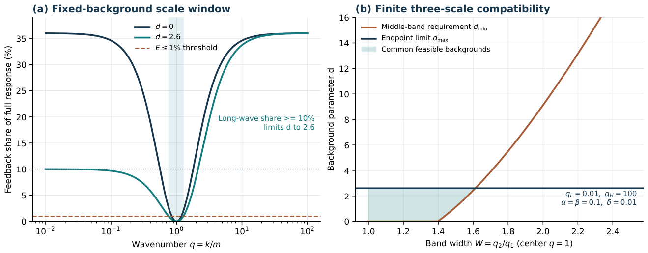
Figure 4.
Inhomogeneous background and probe responses for the localized source. The radial equations determine the background and the full noncommuting kernel determines the feedback fractions. Coordinates and source parameters are normalized; the fractions describe model field feedback, not astronomical gravitational shares.
Figure 4.
Inhomogeneous background and probe responses for the localized source. The radial equations determine the background and the full noncommuting kernel determines the feedback fractions. Coordinates and source parameters are normalized; the fractions describe model field feedback, not astronomical gravitational shares.
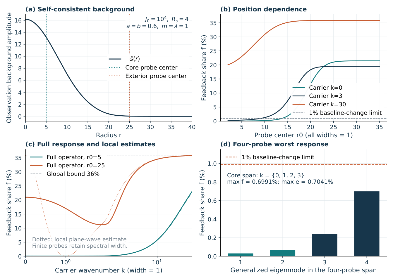
Figure 5.
Internal observation-sector source in the minimal covariant realization. The first three panels show active density, enclosed component mass, and normalized acceleration on the Gaussian-source background of Section 27; the mass is not a total-field fraction, and the acceleration amplitude is uncalibrated. The fourth panel gives the analytical small-amplitude example in which positive feedback accompanies negative active gravitational mass.
Figure 5.
Internal observation-sector source in the minimal covariant realization. The first three panels show active density, enclosed component mass, and normalized acceleration on the Gaussian-source background of Section 27; the mass is not a total-field fraction, and the acceleration amplitude is uncalibrated. The fourth panel gives the analytical small-amplitude example in which positive feedback accompanies negative active gravitational mass.
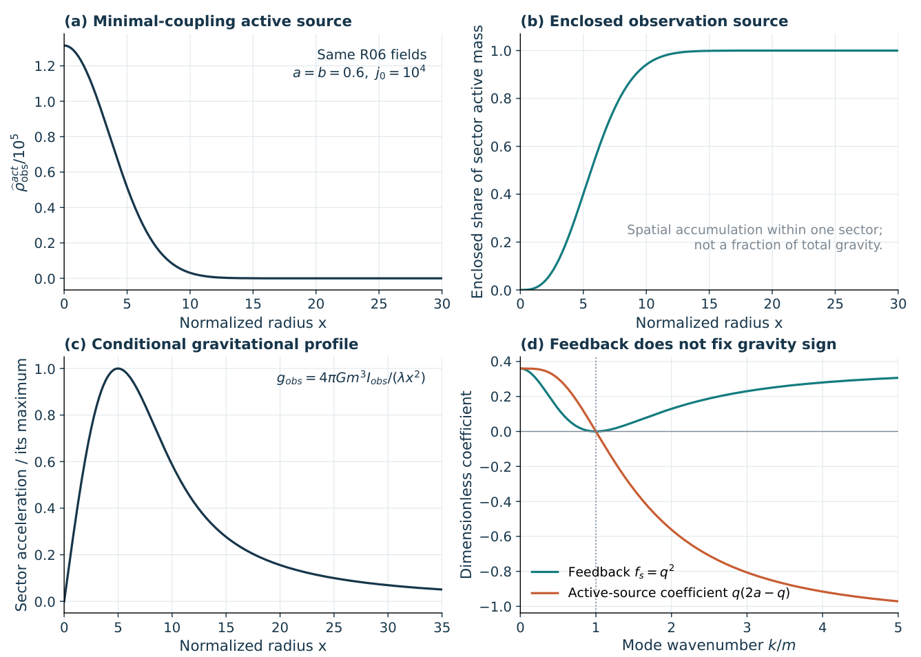
Fit objective and required data. Let denote the measured torque at position j and harmonic , with error , and let and denote the separation and its error. Writing for the field parameters under test and for the apparatus parameters, reproduction of the original analysis uses
The original analysis uses this effective-error fitting criterion, which differs from the full Gaussian negative log-likelihood. A Gaussian model must retain its normalization whenever the variances depend on the estimated parameters, including for independent errors; correlated errors also require off-diagonal covariances. For torque-residual vector r and covariance , the Gaussian model gives
where is a fixed reference covariance and is the contribution from independent calibration measurements. Coverage of a joint admissible region depends on both the statistical model and the interval construction. Replacing the original objective in Eq. (37.67) with this probability model therefore requires a separate justification. The five fitted apparatus parameters concern the horizontal center, separation offset, surface roughness, and angular gain. The remaining geometric and material parameters must likewise be fixed to values measured for the original apparatus.
Figure 6.
Conserved-carrier solutions at fixed parameters: density and free surface (upper left), observation field (upper right), signed enclosed gravitational ratios (lower left), and feedback for a fixed-width probe with mobile or frozen carrier density (lower right). All quantities use the same background. The dimensionless scales are not assigned to actual astronomical or microscopic systems.
Figure 6.
Conserved-carrier solutions at fixed parameters: density and free surface (upper left), observation field (upper right), signed enclosed gravitational ratios (lower left), and feedback for a fixed-width probe with mobile or frozen carrier density (lower right). All quantities use the same background. The dimensionless scales are not assigned to actual astronomical or microscopic systems.
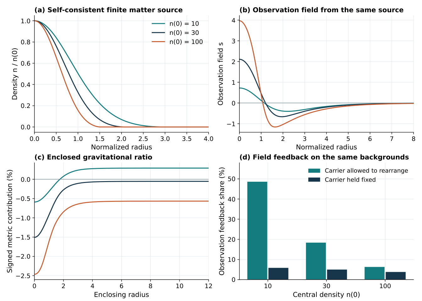
Figure 7.
Physical-scale matching and background validity. Left: fixing and identifying the carrier as protons places all three radii at tens of femtometers. Right: the central equilibrium term omitted when the original profiles are retained at nominal solar compactness. Crosses mark simultaneous proton-mass and solar-radius matching. The curves diagnose mismatch; they are not stellar evolutionary tracks.
Figure 7.
Physical-scale matching and background validity. Left: fixing and identifying the carrier as protons places all three radii at tens of femtometers. Right: the central equilibrium term omitted when the original profiles are retained at nominal solar compactness. Crosses mark simultaneous proton-mass and solar-radius matching. The curves diagnose mismatch; they are not stellar evolutionary tracks.
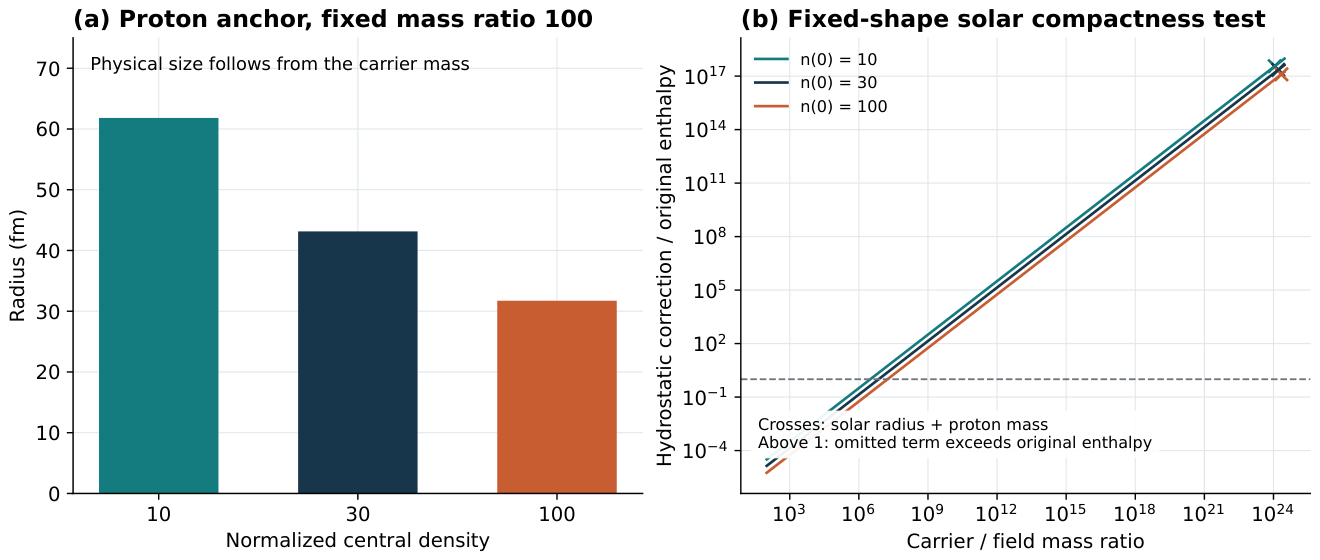
A refit should first reproduce the Newtonian result , . After adding the two-term signal in Eq. (37.41), the apparatus parameters must be optimized under the same calibration constraints at every tested field-parameter point. For a likelihood fit, this optimization is nuisance-parameter profiling [24]. The published summary values give in the accompanying calculation. Only this goodness-of-fit conversion has been reproduced; the 285 individual torque residuals have not. Fixing in advance permits fitting only the common length scale and amplitude of that template. Independent identification of requires both interaction ranges and their relative intensity to be constrained by the data. In the absence of a detection, a joint admissible region should be reported; the intensity ratio, which is undefined at zero amplitude, cannot be assigned the value four.
Limits on identifying the quartic coefficient from linear torque data. Here continues to denote the quartic restoring coefficient, while the Yukawa ranges are denoted by . The zero-background linear template is independent of the quartic coefficient, so
Without an additional prior on , the corresponding row and column of the information matrix for this linear fit vanish; is therefore unidentifiable. A dependence on the coefficient may emerge in the full nonlinear apparatus response, which requires recomputing both the background and instrument readout. The separation scan in the original experiment changes the source geometry; it is not the fixed-profile amplitude scan in Sec. Section 37.15. Nor can torque be identified directly with without a readout map.
The required dataset comprises pointwise torques, uncertainties and positions; geometric and material specifications; the five priors and their correlations; and Newtonian, Yukawa, and magnetic-background templates or records sufficient to reconstruct them. The files run_r17.py and experimental_calibration_R17.json record the summary checks and missing inputs, without field-parameter estimates.
37.18. Numerical Tests of Scale Dependence, Identification, and Readout Maps
The calculations below test Eqs. (37.9)–(37.12) for field feedback and Eqs. (37.20)–(37.21) for gravity. They check analytic consistency and numerical convergence using synthetic inputs, not measured fractions. The action, background, and probe family determine and ; establishing a three-scale ordering also requires the fractions themselves, since derivatives leave integration constants undetermined.
The scale-derivative calculation in run_r10.py uses 160 paths of complex noncommuting positive-definite matrices, using full-matrix solutions and independent five-point differences. The maximum absolute difference is . For 24 paths, the integrated relation has a maximum absolute difference of . At 101 radii, including zeros of the enclosed observation-sector active mass, the signed gravitational formula has a maximum absolute discrepancy of . A further 250 endpoint tests verify the directions of the three-scale threshold inequalities. The matrix paths and analytic densities isolate the algebraic identities.
The inhomogeneous model of Eq. (25.1) provides a test of the action derivatives in run_r11.py. The parameters remain , with a computational radius of 60 and zero Dirichlet boundary conditions. The original Gaussian background source is assigned width while its peak remains . The probe retains center 5 and wavenumber 3, its width becomes , and its norm remains unity. This protocol does not hold the total amount of matter fixed. At , using 7999 interior points, the calculation gives
Background rearrangement reverses the sign of the logarithmic scale derivative predicted from probe variation alone.
Comparison with independently recomputed solutions for neighboring sources gives a relative error of for the background derivative on the fine grid and for the response-kernel derivative. The maximum absolute difference in the fraction derivative is . Refinement through 1999, 3999, and 7999 interior points gives a ratio of successive differences close to ; the fraction derivatives on the two finest grids differ by . The derivative comparison establishes consistency of differentiation, whereas grid refinement tests spatial convergence.
The gravitational numerator uses the same field solution and minimally covariant active source. Both the boundary term and internal-rearrangement term are evaluated at readout radius . The fine-grid relative difference in the derivative is , and the relative difference between two quadrature resolutions is below . The full signed-fraction formula is checked separately by independent integration and finite differences of analytic density functions, with a maximum absolute difference of . Since the original imposed Gaussian source does not specify all masses and pressures of a conserved carrier, the field-solution check reports only the derivative of the active-source numerator. Parameters, contributions, and errors are recorded in verification_results_R11.json.
For 160 complex positive-definite joint kernels, run_r12.py compares the frozen response obtained directly from the energy kernel with its reconstruction from the joint response. The maximum relative difference is , and the maximum absolute difference in the fraction is . Under invertible changes of observation coordinates with consistent calibration of the conjugate source, the fraction changes by at most . A further 200 structural counterexamples verify that the fraction can change while the full physical response remains unchanged; the maximum relative response difference is . A total of 1000 interval checks cover signed gravitational contributions and incompatible field-response intervals. The results are recorded in verification_results_R12.json.
In run_r13.py, independent evaluations of the spatial kernel and torque map give the following comparisons. Across 1000 cases, the full joint-kernel solution and two-branch decomposition differ by at most in relative terms. Direct integration of the undecomposed rational propagator agrees with the analytic spatial kernel at nine radii to a maximum relative error of . At 80 radii, five-point differences of the potential energy agree with the analytic force to a maximum relative error of . For finite geometries, the calculation uses synthetic discrete sources. Pointwise force cross products and angular differences of the total potential energy are compared at 121 angles; the maximum discrepancy divided by the peak torque is . Angular quadrature with 2048 points also verifies the derivative relation between torque and energy harmonics. Section 37.12 discusses the experimental constraints to which this signal map could be applied.
For linear inverse calibration, run_r14.py applies five common amplitude scalings to each of 1000 parameter sets, then reconstructs the parameters from the two spectral branches. The maximum absolute errors in are , and the maximum relative error in is . Across 5000 full joint-kernel solutions, the fraction differs from Eq. (37.47) by at most in absolute terms. The program also rejects 11 types of input that lie outside the selected branch or do not admit an intensity ratio; a nondetection is not interpreted as a calibrated parameter value.
Nonlinear nonidentifiability can be seen by taking in the same action and comparing the uncalibrated values and 10. Their zero-field linear spectra are identical, but their finite-source stationary values are and , respectively. The corresponding homogeneous feedback fractions are and , and the observation-sector active densities are and . The residuals of the original two stationary equations are below . With the carrier unchanged, these solutions demonstrate nonlinear nonidentifiability from linear data; their active densities are not complete gravitational fractions.
The nonlinear calibration calculation in run_r15.py uses a radial Gaussian source of width 4 in a domain of radius 60, with zero Dirichlet boundary conditions. The parameters are ; only the source amplitude and the original quartic coefficient are varied. With 1599 interior points, , , and . Small-amplitude readouts are calculated from the full nonlinear solutions and then used to recover through the cubic formula. As the source amplitude is successively halved from to , the error ratios between the final two levels are and for , respectively, consistent with an truncation error. The final Richardson extrapolations give relative errors of and , respectively.
At fixed , both full solutions satisfy . Equation (37.58) agrees with independent five-point differences to a maximum relative error of ; the derivatives are negative and satisfy the bounds in Eq. (37.59). Inverting these synthetic finite-amplitude readouts recovers with absolute errors below . Predictions at amplitudes , which were not used in the inversion, have a maximum relative response error of . The resulting errors measure inverse consistency within the same discrete model and do not quantify continuum accuracy or experimental uncertainty.
Spatial convergence is checked independently with 799, 1599, and 3199 interior points. At , the ratio of successive readout changes is , and the relative change between the two finest grids is . Using the finest-grid response as a common target, inversion on the two coarser grids gives errors in of and . The coarser-grid bias resolves spatial discretization error that remains hidden in the much smaller same-grid substitution error.
Independent five-point differences in source amplitude reproduce the differential response with a maximum relative difference of . At , the original synthetic system gives
| 1 | 444.6312015 | 441.7424993 | 0.25910793 |
| 10 | 435.0999744 | 419.0347147 | 0.21895847 |
The table gives differential feedback fractions for this source and background. The file verification_results_R15.json records all parameters, stationarity residuals, and errors.
Conclusions
A common action relates observation-field feedback to observation-induced gravity while keeping their definitions distinct. Field feedback compares differential responses with observation-sector perturbations allowed or frozen on the same background; a stable conjugate-response channel gives . The gravitational fraction instead compares components of the active source in one covariant realization and may lie outside because the observation-sector source can have either sign. Shared background equations therefore lead to two calculations with different variations and independent physical inputs.
For comparable source, boundary, and probe families under the same action, scale dependence follows from probe variation, background rearrangement, and, for gravity, the measurement boundary and internal source distribution. The finite-band criteria, scale derivatives, and identification relations derived here make a proposed macroscopic–mesoscopic–microscopic ordering testable. They do not imply a universal pattern of stronger effects at macroscopic and microscopic scales with a weaker mesoscopic regime, nor do scale labels alone determine a fraction.
In the two-field model, independent identification of both spectral branches fixes the linear parameters. A nonlinear conjugate response also fixes the quartic coefficient when the source strength is calibrated and the observation channel is excited. The resulting background gives the field-feedback fraction and observation-sector active source for the chosen source; the full gravitational denominator still requires the actual carrier and support stresses. Independent numerical calculations and spatial-convergence tests support the analytic relations. Physical fractions across the three scale regimes remain to be determined from measurements of the respective systems; the published calibration summaries reproduced here do not supply them.
Appendix A. A Nonlinear Example
The implicit-response and second-order formulas can be checked in the following purely mathematical example. Let
The positive-root branch satisfies , so the local theorem applies for every real O. Direct calculation gives
Differentiating the explicit solution also gives
The two expressions agree identically. At ,
The code below evaluates the derivatives and Schur elimination by independent methods. The resulting discrepancies are floating-point and finite-difference truncation errors, not measurement errors.
import numpy as np
def law(o):
return (-o + np.sqrt(o*o + 4.0))/2
o = 0.4
l = law(o)
a = 2*l + o
d1 = -l/a
d2 = -(2*d1*d1 + 2*d1)/a
h1, h2 = 1e-5, 1e-3
fd1 = (law(o+h1)-law(o-h1))/(2*h1)
fd2 = (law(o+h2)-2*law(o)+law(o-h2))/(h2*h2)
assert abs(fd1-d1) < 1e-9
assert abs(fd2-d2) < 1e-7
H = np.array([[4.0, 0.6], [0.6, 3.0]])
q, u = np.linalg.solve(H, np.array([1.0, 0.0]))
schur = 4.0 - 0.6**2/3.0
assert abs(q - 1.0/schur) < 1e-14
print(l, d1, d2, abs(fd1-d1), abs(fd2-d2))
Appendix B. Computational Methods and Reproducibility
The run.py entry point in the accompanying source package runs directly in a Python 3 environment with NumPy, SciPy, and Matplotlib:
python run.py
xelatex MLO_PODA_English_v1_3_20261027.tex
xelatex MLO_PODA_English_v1_3_20261027.tex
The initial calculations evaluate Eq. (10.11) for the three-outcome probability family and test the two-channel closed-loop phase. At 1501 logarithmically spaced wavenumbers, the full two-by-two matrix solution, Schur expression, and positive spectral decomposition agree to relative discrepancies below . The kinetic and restoring matrices are positive definite, both dispersion branches are stable, and is monotone over the tested range. Central differences reproduce the four derivative terms in Eq. (13.4) to an absolute discrepancy below . Parameters, errors, and tabulated values are saved in verification_results.json; Fig. Figure 1 uses the same calculation.
By default, run.py executes the R03–R09 checks, followed by the R10–R15 scale and identification checks, the R18 same-background counterexample, and the coordinate/source-transformation checks introduced in v1.1. To run only R10–R15, R18, and v1.1, use python run.py –scope-only. The R13 spatial-kernel and torque checks can be run with python run.py –experiment-only, the R14 inverse-calibration checks with python run.py –calibration-only, and the R15 nonlinear-calibration checks with python run.py –nonlinear-calibration-only. The same-background counterexample can be run separately with python run.py –audit-only.
The command python run.py –coordinate-audit-only runs the coordinate and source-transformation tests. For the counterexample in Sec. 37.2, setting gives under a consistent source transformation, but if the source is reset. Four logarithmic scale points test S, , , and their total derivatives under nonorthogonal scale-dependent block transformations. Analytic derivatives and independent finite differences agree to a maximum absolute discrepancy below . The parameters, difference steps, and errors are saved in verification_audit_v1_1.json.
R04 compares analytic cubic roots with independent polynomial root finding, evaluates stationarity residuals at 182 source values, and compares the generalized eigenvalue and analytic spectra, as well as full-matrix and Schur responses. Five-point differences test the source derivatives and third-derivative formulas. Further calculations cover the finite-band thresholds, endpoint maxima, dynamic-kernel identity, and remainder bound for complex z. Background residuals and direct-response errors are below ; spectral and derivative errors are below . The errors and fixed parameters are saved in verification_results_R04.json, with the same equations used for Fig. Figure 2 and Table 2. Numerical units, source ranges, and model parameters are documented in the same file.
R05 tests 600 random scalar responses, 3006 finite three-scale intervals, and 100 response fractions for noncommuting positive-definite matrices, together with monotonicity of the weak-response width on 301 backgrounds. Equation (23.7) is additionally checked using an analytic positive mass function and five-point differences, and Eq. (23.8) by independent integration. The maximum discrepancy between scalar direct inversion and the analytic fraction is ; the maximum matrix-fraction error is , and the maximum absolute error in the radial gravitational derivative is . For the three-outcome probability family used in the main text, choosing , , , gives a total variation of and half the Fisher path length of , satisfying Eq. (24.2). Parameters, actual errors, and the two sets of feasible-region results are recorded in verification_results_R05.json; Fig. Figure 3 is generated by the same script.
The R06 calculation, run_r06.py, solves for the unique radial background before evaluating the full response. The resulting data are saved in verification_results_R06.json and used for Fig. Figure 4. Besides the grid and boundary studies described in the main text, five-point differences test Eq. (25.5) with relative error . Separate solutions at nearby source amplitudes test Eq. (25.6) with relative error . The derivative is local to the chosen background. An analytic smooth potential tests Eqs. (28.3) and (28.1).
R07 verifies Eq. (29.4) by direct contraction of the Hilbert stress tensor for 300 sets of random spacetime gradients, with a maximum absolute discrepancy of . Reusing the R06 background solver, the internal-source calculation compares direct integration with the boundary-inclusive integral identity, varies the grid and outer boundary, and solves a separate counterexample with negative active source. The divergence and surface terms from nonminimal coupling are independently checked using analytic test functions, with a maximum absolute discrepancy of . The results are saved in verification_results_R07.json, and Fig. Figure 5 is generated by the same script.
In R08, carrier_r08.py solves for the background of the conserved fluid and two scalar fields. The companion script run_r08.py evaluates stresses, enclosed masses, constrained spectra, and feedback for the two carrier readouts. The background is obtained from a radial boundary-value problem with the origin singularity regularized: both field derivatives vanish at the origin, and decay conditions for the two mass modes are imposed at the outer boundary. The free surface is determined by the density first integral. Results are saved in verification_results_R08.json; Fig. Figure 6 and Table 4 use the same parameters and solution. The script also checks the exact threshold in Eq. (34.6) and the fixed-particle-number constraint residuals in both the full and reference responses.
The R09 calculation in run_r09.py recomputes the background independently for the calibration and potential-difference tests of Sec. 36. Results, sources of constants, and applicability conditions are recorded in verification_results_R09.json.
The scale-identity tests of Sec. Section 37 run in run_r10.py. Results are saved in verification_results_R10.json. Their fixed finite-dimensional matrices do not test changing constraint spaces or infinite-dimensional operator domains.
The script run_r11.py reuses the R06 background solver at neighboring sources, with two finite-difference steps, three spatial grids, and two quadrature resolutions. Analytic densities separately test the full gravitational fraction.
The script run_r12.py uses synthetic positive-definite kernels for the joint-response reconstruction, coordinate-invariance, nonidentifiability, and interval tests reported above.
The script run_r13.py compares the full kernel, its oscillatory Fourier integral, and the analytic potential and force, and evaluates synthetic finite-source torques by two methods. The source specification, errors, and force-difference zero are saved in verification_results_R13.json. No data from Ref. [23] are read.
The script run_r14.py writes inverse-calibration errors, feasibility checks, and nonlinear-identifiability counterexamples to verification_results_R14.json.
The script run_r15.py solves the radial nonlinear stationarity equations for the calibration and differential-feedback tests. Three grids distinguish spatial error from fixed-grid inverse consistency; verification_results_R15.json records the readouts and errors.
The script run_r18.py evaluates the integrated observation-sector active source and full differential response to probe on three nonzero small-amplitude backgrounds of Eq. (30.1). At , all three give and . Successive amplitude halvings reduce the feedback’s deviation from its discrete zero-background value by factors of and . The fractions from the full block solution and independent Schur elimination differ by less than . The results in verification_results_R18.json test the sign counterexample on the same nonzero background and its expansion. They establish fixed-grid consistency, without providing a continuum error bound or measured fraction.
The published experimental calibration quantities can be checked separately:
python run.py –published-calibration-only
The file experimental_calibration_R17.json records the published measurement summaries, first-order uncertainty-propagation assumptions, and missing inputs.
Appendix C. Physical Inputs and Sources
The four-quadrant relations, MLO hierarchy, and physical–observation dual-axis terminology used here are defined in Sec. 1. The mathematical objects , , , and the information criteria are defined under the regularity and comparison conditions given in the main text.
The low-energy geometry, mixed-source allocation, and exchange relations are specified in the main text. The active source uses the chosen minimal covariant realization; it is not fixed by the flat-spacetime action alone.
The quartic potential, isentropic-fluid law, and source coupling are constitutive choices. Applying them to a physical system requires independent material, source, boundary, and readout data, with stability and weak-field checks; unit conversion alone is insufficient, as the proton/solar matching example shows.
Reference [6] supplies the classical information-geometric background, while Refs. [7,8] concern coherent-state geometry and phase comparison. References [18,19] provide the physical constants used for unit conversion and scale matching. Reference [23] supplies the apparatus readouts, data sources, and single-term Yukawa constraints from the short-range gravity experiment. The calibration summaries are distinguished from the synthetic calculations throughout; no two-term experimental fit is reported.
References
- X. Meng, The Natural Dual-Axis Structure of Observation: Categorical Foundations and Consequences for Quantum Theory, Preprints.org (2026), version 4, preprint (not peer-reviewed). 202609.0572. v4.
- Blackwell, D. Equivalent comparisons of experiments. Ann. Math. Stat. 1953, 24, 265–272. [Google Scholar] [CrossRef]
- C. E. Shannon, A mathematical theory of communication. Bell Syst. Tech. J. 1948, 27, 379–423. [CrossRef]
- Kullback, S.; Leibler, R. A. On information and sufficiency. Ann. Math. Stat. 1951, 22, 79–86. [Google Scholar] [CrossRef]
- Fedotov, A. A.; Harremoës, P.; Topsøe, F. Refinements of Pinsker’s inequality. IEEE Trans. Inf. Theory 2003, 49, 1491–1498. [Google Scholar] [CrossRef]
- Amari, S.-I. Differential geometry of curved exponential families—curvatures and information loss. Ann. Stat. 1982, 10, 357–385. [Google Scholar] [CrossRef]
- Provost, J. P.; Vallée, G. Riemannian structure on manifolds of quantum states. Commun. Math. Phys. 1980, 76, 289–301. [Google Scholar] [CrossRef]
- Berry, M. V. Quantal phase factors accompanying adiabatic changes. Proc. R. Soc. A 1984, 392, 45–57. [Google Scholar] [CrossRef]
- X. Meng, The Phase Transport Fundamental Equation on the Physical–Observation Dual-Axis Structure, Preprints.org (2026), version 2, preprint (not peer-reviewed). 202608.1128. v2.
- Feshbach, H. Unified theory of nuclear reactions. Ann. Phys. 1958, 5, 357–390. [Google Scholar] [CrossRef]
- Zwanzig, R. Memory Effects in Irreversible Thermodynamics. Phys. Rev. 1961, 124, 983. [Google Scholar] [CrossRef]
- Mori, H. Transport, Collective Motion, and Brownian Motion. Prog. Theor. Phys. 1965, 33, 423–455. [Google Scholar] [CrossRef]
- Galley, C. R. Classical Mechanics of Nonconservative Systems. Phys. Rev. Lett. 2013, 110, 174301. [Google Scholar] [CrossRef] [PubMed]
- Tolman, R. C. On the Use of the Energy-Momentum Principle in General Relativity. Phys. Rev. 1930, 35, 875. [Google Scholar] [CrossRef]
- Meng, X. Physical–Observation Dual-Axis (PODA) Relativity: Continuous Observation Fields, Recovery of General Relativity, and Experimental Tests, Preprints.org (2026), version 1, preprint (not peer-reviewed). 202609.1261. v1.
- Callan, C. G., Jr.; Coleman, S.; Jackiw, R. A new improved energy-momentum tensor. Ann. Phys. 1970, 59, 42–73. [Google Scholar] [CrossRef]
- Brown, J. D. Action functionals for relativistic perfect fluids. Class. Quantum Gravity 1993, 10, 1579–1606. [Google Scholar] [CrossRef]
- Prša, A.; et al. Nominal Values for Selected Solar and Planetary Quantities: IAU 2015 Resolution B3. Astron. J. 2016, 152, 41. [Google Scholar] [CrossRef]
- Mohr, P. J.; Newell, D. B.; Taylor, B. N.; Tiesinga, E. CODATA recommended values of the fundamental physical constants: 2022. Rev. Mod. Phys. 2025, 97, 025002. [Google Scholar] [CrossRef]
- Hoyle, C. D.; Kapner, D. J.; Heckel, B. R.; Adelberger, E. G.; Gundlach, J. H.; Schmidt, U.; Swanson, H. E. Submillimeter tests of the gravitational inverse-square law. Phys. Rev. D. 2004, 70, 042004. [Google Scholar] [CrossRef]
- Kapner, D. J.; Cook, T. S.; Adelberger, E. G.; Gundlach, J. H.; Heckel, B. R.; Hoyle, C. D.; Swanson, H. E. Tests of the Gravitational Inverse-Square Law below the Dark-Energy Length Scale. Phys. Rev. Lett. 2007, 98, 021101. [Google Scholar] [CrossRef] [PubMed]
- Tan, W.-H.; et al. Improvement for Testing the Gravitational Inverse-Square Law at the Submillimeter Range. Phys. Rev. Lett. 2020, 124, 051301. [Google Scholar] [CrossRef] [PubMed]
- Lee, J. G.; Adelberger, E. G.; Cook, T. S.; Fleischer, S. M.; Heckel, B. R. New Test of the Gravitational 1/r2 Law at Separations down to 52μm. Phys. Rev. Lett. author manuscript; Supplemental Material. 2020, 124, 101101. [Google Scholar] [CrossRef] [PubMed]
- Cowan, G.; Cranmer, K.; Gross, E.; Vitells, O. Asymptotic formulae for likelihood-based tests of new physics. Eur. Phys. J. C 2011, 71, 1554. [Google Scholar] [CrossRef]
Figure 1.
Dependence of the inferred enhancement on the reference response, with all parameters fixed. Left: the change relative to the frozen-observation baseline is larger at both spectral ends. Right: multiplying the same response by gives a strictly monotone curve, excluding low-wavenumber enhancement relative to a fixed baseline. The shaded band identifies relative errors of at most in the left panel.
Figure 1.
Dependence of the inferred enhancement on the reference response, with all parameters fixed. Left: the change relative to the frozen-observation baseline is larger at both spectral ends. Right: multiplying the same response by gives a strictly monotone curve, excluding low-wavenumber enhancement relative to a fixed baseline. The shaded band identifies relative errors of at most in the left panel.
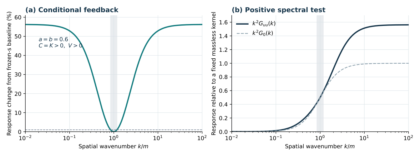
Figure 2.
Analytic responses of the same nonlinear model. Left: the total background and differential responses are both suppressed as the source grows, but their values differ; the vertical dashed line marks the differential-error threshold for . Right: increasing the source weakens feedback at finite wavenumbers, while the static high-wavenumber limit remains . Every curve uses .
Figure 2.
Analytic responses of the same nonlinear model. Left: the total background and differential responses are both suppressed as the source grows, but their values differ; the vertical dashed line marks the differential-error threshold for . Right: increasing the source weakens feedback at finite wavenumbers, while the static high-wavenumber limit remains . Every curve uses .
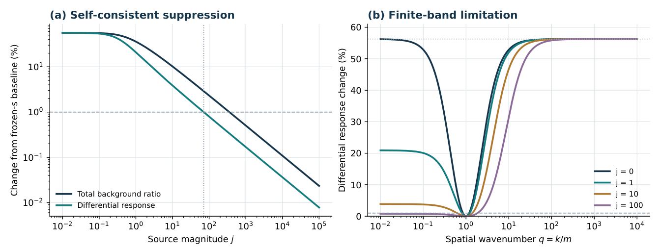
Table 1.
Dimensionless two-state calculation at fixed parameters, checked against the full two-by-two system. The entries are model values, not measurements.
Table 1.
Dimensionless two-state calculation at fixed parameters, checked against the full two-by-two system. The entries are model values, not measurements.
| 0.01 | 0.359856 | 1.562149 | 56.2149% |
| 0.10 | 0.345884 | 1.528780 | 52.8780% |
| 1.00 | 0 | 1 | 0 |
| 10.00 | 0.345884 | 1.528780 | 52.8780% |
| 100.00 | 0.359856 | 1.562149 | 56.2149% |
Table 4.
Two types of contribution on self-consistent backgrounds with the same parameters. Field feedback is measured with ; the gravitational column is the signed ratio of full-domain enclosed masses and has not been calibrated to an actual system.
Table 4.
Two types of contribution on self-consistent backgrounds with the same parameters. Field feedback is measured with ; the gravitational column is the signed ratio of full-domain enclosed masses and has not been calibrated to an actual system.
| Free-surface radius | (%) | (%) | (%) | |
|---|---|---|---|---|
| 10 | 2.9393 | 48.59 | 5.83 | +0.2900 |
| 30 | 2.0512 | 18.34 | 4.98 | -0.0536 |
| 100 | 1.5088 | 6.29 | 3.79 | -0.5670 |
Table 5.
Incompatible physical calibrations when the example value is retained. The two columns fix different physical inputs; they are not two unit representations of one object.
Table 5.
Incompatible physical calibrations when the example value is retained. The two columns fix different physical inputs; they are not two unit representations of one object.
| [r]Radius for a | ||
|---|---|---|
| proton carrier (m) | [r]Carrier rest energy at the | |
| nominal solar radius (eV) | ||
| 10 | ||
| 30 | ||
| 100 |
Disclaimer/Publisher’s Note: The statements, opinions and data contained in all publications are solely those of the individual author(s) and contributor(s) and not of MDPI and/or the editor(s). MDPI and/or the editor(s) disclaim responsibility for any injury to people or property resulting from any ideas, methods, instructions or products referred to in the content. |
© 2026 by the authors. Licensee MDPI, Basel, Switzerland. This article is an open access article distributed under the terms and conditions of the Creative Commons Attribution (CC BY) license (http://creativecommons.org/licenses/by/4.0/).
Copyright: This open access article is published under a Creative Commons CC BY 4.0 license, which permit the free download, distribution, and reuse, provided that the author and preprint are cited in any reuse.