
Submitted:
22 October 2026
Posted:
23 October 2026
You are already at the latest version
Abstract
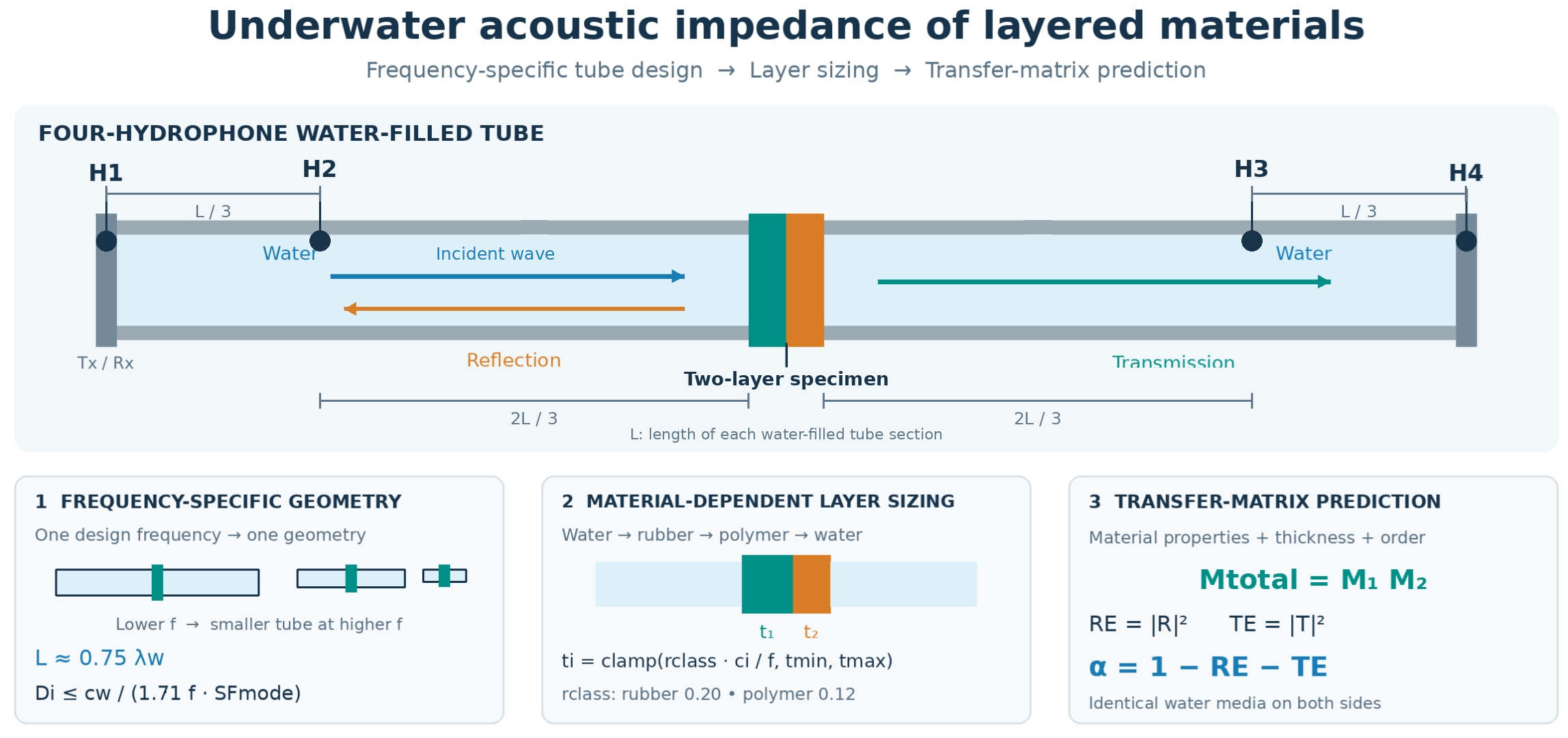
The paper presents an integrated methodology for designing water-filled acoustic impedance tubes and interpreting measurements of the acoustic impedance of single- and multilayer polymer and elastomer in underwater conditions. The first part consolidates a family concept of three circular, water-filled tubes dedicated to different frequencies, respectively, based on a plane-wave criterion, wall-stiffness constraints and a four-hydrophone configuration with two end-cap sensors and two mid-span sensors positioned symmetrically around the sample. The proposed geometry sizing algorithm derives tube length, inner diameter, wall thickness, tube material selection and deaeration requirements for the laboratory stand. The second part links the hardware proposal to the physics requirements in water by recalling the relations between sound pressure, par-ticle velocity and specific impedance. Moreover, there is a proposal for formulating reflection, transmission and absorption coefficients for normal incidence at water–solid plates. Using a Transfer-Matrix Method (TMM), single-layer and multilayer configurations such as water–elastomer–water and water–rubber–polymer–water are modelled with complex wavenumbers to account for frequency-dependent phase velocity and attenuation. This approach enables prediction of resonance bands and broadband absorption behaviour in the 10–100 kHz range.
Keywords:
underwater acoustic impedance
; water-filled impedance tube
; multilayer polymer specimens
; transfer matrix method
; two-layer materials in water
1. Introduction
The characterisation of acoustic wave interaction with solid materials in water is an important problem in underwater acoustics, naval engineering and the design of protective and functional material systems. In contrast to air-borne acoustics, measurements performed in water are strongly affected by the much higher density and acoustic impedance of the surrounding medium, which significantly changes reflection, transmission and absorption phenomena at water–solid interfaces. This makes the direct transfer of standard air-filled impedance-tube concepts insufficient, especially when the objective is to study polymer, elastomer, composite or multilayer specimens under conditions representative of underwater applications.
For this reason, there is a clear need for research that combines two complementary aspects, i.e. the physically consistent design of water-filled acoustic impedance tubes and the reliable interpretation of the acoustic response of finite-thickness material layers immersed in water. The main objective of this study is to develop an integrated approach that links the preliminary design of a family of water-filled impedance tubes with the analysis of the acoustic impedance of two-layer material systems in underwater conditions. The work aims to define frequency-specific tube geometries, and deaeration methods, and to connect these design choices with a TMM-based description of reflection, transmission and absorption in layered specimens. A further goal is to establish sample-sizing rules that account for the acoustic properties of different material classes.
The theoretical basis for this area was established in the general acoustics literature. Randall and Maxwell discussed the relations between sound pressure, particle velocity, reflection, and transmission [1]. Lurton and Jackson described the propagation of sound in water, and the practical implications of attenuation and boundary interaction in submerged systems [2]. Jacobsen et al. presented an elementary introduction to acoustic fundamentals and noise-control concepts that remain directly relevant to water-filled impedance tubes [3].
The standardized methodological background of impedance-tube research is mainly defined by ISO and ASTM documents. ISO 10534-2 established the standing-wave-ratio method for determining the sound absorption coefficient and impedance in impedance tubes [4]. ASTM E1050 provided the equivalent standardized framework widely used in engineering laboratories for normal-incidence acoustic measurements [5]. In addition, ASTM E2611 extended tube-based methodology toward transmission-loss measurements, which is particularly relevant for layered underwater barriers and through-transmission fixtures.
Bobber and Beatty presented an impedance tube for underwater sound transducer evaluation [6]. Their work is important because it demonstrated that underwater impedance-tube concepts are not merely theoretical analogies to air acoustics, but can be built as dedicated laboratory tools for submerged devices. Another historically important contribution is the study titled Measurement of Acoustic Impedances of Surfaces in Water [7]. This line of work established the practical feasibility of controlled normal-incidence acoustic characterization directly in a water medium, which remains one of the core motivations for current research on submerged polymer and multilayer specimens.
The literature has also shown growing interest in extending underwater impedance-tube techniques to realistic service environments [8]. This work demonstrated that underwater impedance measurements can be adapted to pressure-dependent conditions, which is important for marine applications where the acoustic response of elastomers, polymers, or porous systems may vary with depth.
The second major body of literature focuses on modelling wave interaction with finite-thickness plates and layered media. Lee and Xu proposed a modified transfer matrix method for predicting transmission loss of multilayer acoustic materials [9]. Their work is directly applicable to submerged layered specimens when the surrounding medium is water rather than air. Broader methodological support for the Transfer Matrix Method (TMM) was later provided by Verdière and co-authors, who applied the transfer matrix method to parallel assemblies of sound-absorbing materials and showed how non-uniform layered systems can be represented within an extended matrix formalism [10].
Several authors specifically addressed polymeric and composite materials. Fahad and Al-Jadiri studied the acoustic impedance of polymer–polymer hybrid composites intended as insulating materials, demonstrating how composition and internal structure affect acoustic response [11]. Nastac et. al. investigated the acoustic performance of expanded-perlite composites reinforced with waste and natural polymers, showing the ongoing relevance of impedance-based methods for evaluating heterogeneous soft materials [12]. Although these studies are not always underwater-specific, they are methodologically valuable because they analyse the connection between microstructure, losses, and effective acoustic behaviour.
Underwater layered absorbers and metamaterials form another highly relevant cluster of literature. Qu and co-authors presented an underwater metamaterial absorber with an impedance-matched composite configuration, demonstrating that carefully designed composite layering can significantly improve underwater absorption [13]. Liu and co-authors evaluated a hybrid underwater sound-absorbing megastructure using the transfer matrix method. They showed that combined mechanisms, including viscoelastic substrate response and microperforated effects, can produce high absorption in the kilohertz range [14]. These studies are especially important for the present topic because they demonstrate the application of the TMM-based design.
The metrological literature also emphasizes that specimen mounting details can strongly influence measured impedance. A dedicated study on the influence of the interstice of water around a sample in an impedance tube demonstrated that even a thin water gap can distort the apparent acoustic properties of the specimen [15]. Additional methodological context is provided by Hiremath et. al., who reviewed acoustic impedance measurement techniques and prospects across different measurement systems and confirmed that impedance measurement is moving toward more specialized water-filled tubes [16]. Mihajlov and other co-authors reviewed methods for measuring sound absorption coefficients in impedance tubes, confirming the metrological importance of proper design configurations [17].
Taken together, the literature shows that the present research area is scientifically justified and technically timely. Against this background, the present thematic direction occupies a distinct position in the literature: it does not treat tube design and layered-material modelling as separate issues, but instead integrates them into one engineering methodology. Such an approach is necessary for the reliable determination of the underwater acoustic impedance of two-layer materials, especially when the final goal is to develop practical underwater barriers, sound-absorbing coatings, polymer–elastomer layered specimens, or other functional structures for marine engineering applications.
The expected utility of the obtained results is both methodological and application-oriented. From a metrological standpoint, the proposed framework may support the development of repeatable laboratory procedures for determining the underwater acoustic properties of engineered materials, including polymers, elastomers, composites and metal-backed layered systems. From an engineering standpoint, the results may be used in the design and optimisation of underwater acoustic barriers, sound-absorbing coverings, layered protective elements and material systems intended for defense of marine infrastructure-related applications, where control of reflection, transmission and energy dissipation in water is required.
2. Acoustic Impedance in Water and Solid Layers
The basic parameters characterizing the subject of this work require a brief reminder of the basic relationships in the field of underwater acoustics, i.e. pressure, sound velocity and specific impedance in water. An acoustic wave in water is described by the wave equation for pressure p(r,t) as follows: [16,18].
where c is the speed of sound in the given medium.
For a plane harmonic wave defined as:
and the corresponding particle velocity defined as:
The relation holds, where the specific acoustic impedance is:
where, for freshwater, Zw ≈ 1.485 MRayl (ρ ≈ 1000 kg/m³, c ≈ 1490 m/s) [3,19]. For underwater polymers (including POM/polyacetal), the impedance is typically of the order of several MRayl, higher than in water, which leads to a significant impedance mismatch and strong reflection at a smooth, stiff plate [20].
Let us now consider the issue of Reflection and transmission at the water–polyacetal interface. For a plane wave incident normally on the interface between two media with impedances Z0 (water) and Z1 (polyacetal), the amplitude reflection coefficient is:
and the amplitude transmission coefficient is:
The power (energy) reflection coefficient is |R|2, and the power transmitted into the material is: for two fluids; for a solid the description is more complex, but the principle of energy conservation remains valid [18]. When Z1≫Z0, then |R| → 1, i.e. almost all energy is reflected (low absorption for a thin, stiff plate without internal losses) [18].
Let's now consider the example of single-layer propagation and damping in a polyacetal. Upon entering the plate, the wave changes its speed and wavelength and undergoes internal damping (viscoelastic losses) [20]. In a lossy medium, the wavenumber is complex:
Here, cp(f) is the longitudinal phase velocity in the material, αatt ≥ 0 is the amplitude attenuation coefficient expressed in Np/m, and j2 = −1. The time-harmonic convention ejωt is used throughout.
The pressure in the material at depth x decays exponentially:
which corresponds to an amplitude decay factor e−αx and a power decay factor e−2αx [16]. For a plate of thickness g = 0.03 m at high frequencies, which gives a shorter wavelength and higher αatt(f), the material behaves as significantly more absorbing, whereas at low f, i.e. small α, thickness small compared to wavelength, internal attenuation is weaker.
Next, consider the transmission of an acoustic wave through a plate of finite thickness. In the case of a plane wave incident from water onto a flat plate with impedance Zs, wavenumber ks, and thickness g, immersed in water (water–plate–water), the Transfer Matrix method (TMM) is used [12,21]. The input impedance of the plate (seen from the water side) is:
for an elastic plate treated as a 1D layer under normal incidence. The reflection coefficient of the whole layer, not just the bare interface, is then:
and the absorption coefficient, for no further transmission, is α = 1 − |Rlayer|2. In a water–plate–water system, part of the energy is transmitted, and the transmission through the entire layer must also be taken into account [13]. Thickness resonances occur when ksg ≈ nπ, at which the plate can become more transparent (high transmission) or more absorbing, depending on internal losses and impedance matching.
Energy absorption in the material quantifies the fraction of energy that is converted in the material primarily into heat in the forms of viscoelastic friction, microcracking, etc [21]. The absorption coefficient under normal incidence is defined as:
where |R|2 is the fraction of reflected energy and |T|2 is the fraction of energy transmitted beyond the barrier (after accounting for impedance changes) [21]. In a simple water-filled impedance tube experiment, α can be obtained, for example, from the maximum and minimum pressure in the standing wave:[12]
which illustrates the relationship between reflection and absorption [17].
3. Design Concept of Water-Filled Impedance Tubes
This work proposes a concept for a family of water-filled acoustic impedance tubes dedicated to measurements at different frequencies. It uses two identical tube sections with a sample mounted between them and a four-hydrophone arrangement with H1 and H4 in the end caps and H2 and H3 positioned at two-thirds of the single-tube length from the sample on each side – see Figure 1. The design scripts in MATLAB and calculations assume a one-frequency vs one-geometry philosophy because the plane-wave condition in a circular duct rapidly forces smaller tube diameters as frequency increases. In contrast, wall compliance in water-filled tubes simultaneously drives the need for relatively stiff and thick walls.
In each tube section, the pressure field is modelled as the superposition of forward- and backward-propagating plane waves. The two hydrophones on the left (H1 in the end cap, H2 at 2L/3 from the sample) provide a pair of pressure measurements p1(f), p2(f) at known positions, which are used to solve for the amplitudes of the incident and reflected waves in the left tube. Similarly, the two hydrophones on the right (H3 at 2L/3, H4 in the end cap) provide p3(f), p4(f), from which the forward (transmitted) and backward waves in the right tube are obtained. Once the complex incident, reflected and transmitted amplitudes are reconstructed, the amplitude coefficients R(f) and T(f) follow directly, and the energy coefficients:
are computed in the usual way.
This project conceptually is a four-sensor extension of the standard two-microphone transfer-function method. In the left tube, the two pressures define the incident–reflected pair, and in the right tube, the two pressures define the transmitted–reflected pair. The use of four hydrophones allows a symmetric treatment of both sides of the sample. This supports an inverse problem for layered specimens and sensitivity analysis to sensor phase and positioning errors.
The design approach utilizes the standard impedance tube principle of reconstructing incident, reflected, and transmitted wave fields based on pressure measurements at known positions. A new feature of the tube design is the introduction of a four-hydrophone system suitable for aqueous media instead of two sensors. Considering the recommendations of ISO 10534-2 and ASTM E1050 as the normative reference framework for impedance measurements with a transfer function, this solution treats the proposed water-filled system as a research adaptation, rather than a replica of a standard air-filled tube [4,5,22]. For the initial geometry sizing, the core assumptions used across the attached scripts are the following:
- Each operating frequency is assigned its own dedicated tube geometry.
- The single-tube length is initially set to 0.75 of the wavelength in water. In classical wave theory in acoustic tubes, the length of the tube closed at one end and open at the other for the fundamental mode is approximately λ/4. In impedance tubes operating in air, the length of the measuring section is often chosen as a fraction of the wavelength, e.g., λ/4 or slightly more, to obtain a well-developed wave state without entering higher transverse modes.
- The inner diameter is limited by a plane-wave criterion in a circular tube, implemented in the interactive script as dinner=cwater/(1.71 SFmode∙ f) with an initial modal safety factor of 1.8 up to 1.5.
- Hydrophones H2 and H3 are positioned at 2L/3 from the sample, whereas H1 and H4 are integrated in the end caps.
- The sample diameter is smaller than the inner diameter of the pipe by the total assembly clearance, and the seal is made using O-ring technology without interference fit.
- The values L=0.75 and assumed in the design are calculated as initial geometry parameters of the device design and may be optimised in the future.
A simplified calculation algorithm can be formulated as follows:
- Select the design frequency and water properties.
- Compute wavelength in water, λ=cwater/f.
- Analyse and compute the preliminary single-tube length, L=0.75λ, to obtain a compact but still wave-resolving geometry.
- The inner diameter must be calculated based on the plane wave criterion, using a safety factor to protect against higher-order modes.
- The selection of the tube wall thickness should take into account the wall thickness that can be technologically produced, and be adjusted upward for tube materials with lower stiffness, e.g. aluminium.
- Based on the technological data sheets of the transducers and vent valves, determine the thickness of the plug, the geometry of the hydrophone socket and the thread parameters of the vent channels.
- For a portfolio of test sample materials, calculate the longitudinal wave velocity and acoustic impedance, then determine the sample thickness based on the material class rule related to the wavelength fraction in the sample. Include lower and upper limits for performance and production realism.
These recommendations refer to ISO 10534-1, ISO 10534-2, and ASTM E1050 as the primary standards for impedance tube measurements and the transfer function method. In this work, these standards were treated as a conceptual measurement base, with the actual equipment viewed as a test platform requiring additional validation.
Technical analysis of the tube materials offers carbon steel, stainless steel 316L, and aluminum 6082-T6 as candidates. All three are workable at the preliminary-design stage, but they do not offer the same performance when corrosion resistance, stiffness, mass, and production realism are evaluated together. Preferred material by frequency family is presented in Table 1.
4. Engineering Design of Frequency-Specific Tube Geometry
The design of a water-filled acoustic impedance tube requires a physically justifiable geometry that ensures plane wave propagation and remains technologically feasible. In the present work, a MATLAB interactive script is used to implement a preliminary sizing procedure for a family of tubes dedicated from 1000 Hz to 30000 Hz. In this study, the decision was made to analyse the tube geometry for three frequencies: 1 kHz, 5 kHz, and 30 kHz. The script consolidates the core design algorithm, including the one-frequency–one-geometry philosophy. The plane-wave criterion in a circular duct and wall-thickness rules are transferred into an interactive engineering tool that outputs key geometric parameters and visualisations. The idea is that, for each design frequency, the tube length, inner diameter, wall thickness, end-cap geometry, and hydrophone positions should be chosen such that higher-order modes are minimised. Higher-order modes are minimized and practical features such as venting and sample mounting are accommodated without excessive distortion of the acoustic field. Because water has high density, and acoustic impedance, the tube walls must be significantly stiffer and thicker than in air-filled designs.
4.1. Calculation Algorithm for Tube Length and Inner Diameter
The interactive script begins by requesting or defining the design frequency f and water properties, i.e. density ρw and sound speed cw, corresponding to fresh water at the chosen temperature, which in the report is 15 °C. From these values, the acoustic wavelength in water is computed as:
Hence, it was decided that the length of a single tube L on one side of the sample is set to a constant fraction of the wavelength L≈0.75λw was assumed, which gives a compact but at the same time resolved wave geometry, allowing sufficient spatial separation of the hydrophones from the sample. The inner tube’s diameter Di is determined from a plane-wave criterion in a circular duct. In the MATLAB script, this is implemented through an inequality of the form:
where the factor 1.71 corresponds to the classical cut-off condition for the first non-planar mode in a rigid circular waveguide and SFmode is a safety factor against higher-order modes, in the range 1.5–1.8. The paper proposes a plane-wave criterion based on the cutoff frequency condition for the first higher-order mode in a rigid circular waveguide. This assumption requires perfectly rigid tube walls, which is acceptable in theoretical analyses. The proposal complies with the requirements of the ISO 10534-2 and ASTM E1050 standards regarding the design of impedance tubes. For water-filled tubes with large diameters and relatively thin walls, the actual boundary condition deviates from the assumption of wall rigidity. The actual cutoff frequency for non-plane modes may be lower than the value predicted for a rigid tube. This effect is particularly important when the tube walls are made of lower-stiffness materials e.g. aluminium or when the diameter-to-thickness ratio is high, because wall motion couples to the water column and modifies the modal structure. In the present design, the risk of wall-compliance effects is mitigated at the preliminary stage in two ways i.e. by using a modal safety factor, which moves the operating point away from the rigid-wall cut-off and by selecting relatively thick walls and favouring high-stiffness materials like the carbon steel or stainless steel 316L.
The interactive tool calculates geometric data for a selected frequency and provides the inner diameter that ensures the tube operating point below the onset of higher-order modal propagation. By applying the plane wave criterion to the geometry dimensioning, the MATLAB script ensures the tube cross-section is consistent with one-dimensional transfer function analysis and TMM-based layered sampling.
4.2. Wall Thickness and End-Cap Geometry
The wall thickness of the water-filled impedance tube must satisfy two simultaneous requirements: ensuring rigidity under water-loading conditions and allowing for fabrication using available technologies and materials.
The inner diameter Di is determined for successive frequencies by applying the plane-wave criterion for circular ducts and a safety factor to prevent the occurrence of higher-order modes. The outer diameter and wall thickness are calculated based on the wall-thickness-to-diameter ratio and a stiffness correction factor. This approach ensures that the diameter-to-wall-thickness ratio does not result in operation within a range where elastic wall deformation would influence the acoustic field during measurements. This necessitates a thick-walled, high-rigidity design—for instance, using 316L stainless steel.
The dimensions of the end caps are selected to be a specific multiple of the tube's wall thickness, typically tcap ≈ 1,2∙twall. This ensures adequate bending rigidity at the hydrophone mounts and venting channels, while preventing deformation caused by acoustic excitation.
4.3. Geometry of the Four-Hydrophone Configuration
The four-hydrophone configuration is chosen to enable symmetric reconstruction of incident, reflected and transmitted waves by extending the classical two-sensor transfer-function method. In the implemented algorithm, hydrophones H2 and H3 are positioned at distances xH2 = xH3 = 2L/3 from the sample on each side, while H1 and H4 are flush-mounted in the end caps at the distal ends of the tube sections. Hydrophone H1 operates as a combined transmitter and receiver. These positions are treated as preliminary symmetric choices. The initial design assumptions assume that they should be optimised in future iterations by sensitivity analysis of the four-sensor inverse problem, including phase uncertainty, etc. Consequently, the axial separation within each hydrophone pair is s = L/3. This arrangement is a preliminary design choice rather than an experimentally validated optimum. The usable frequency range remains to be established through conditioning and sensitivity analyses accounting for hydrophone phase mismatch, positioning tolerances and deviations from the ideal plane-wave model.
4.4. Technological Feasibility and Production Constraints
A four-hydrophone configuration was selected to enable the symmetrical reconstruction of incident and reflected waves. Moreover, it needs quite different manufacturing technology. The low-frequency geometry, with its large internal diameter and long tube, creates a heavy body with sample, and water. This device requires a rigid support frame, sample holder, and precise assembly. The high-frequency tubes, over 3 kHz are easier to produce. Its inner diameter is compatible with standard precision machining, and conventional hydrophone ports. Wall thickness is easier to produce, and overall mass and size remain suitable for laboratory use without extraordinary handling equipment. Manufacturing problems begin for the tube with a dedicated frequency above 30 kHz, where the calculated inner diameter of the tube is below 20 mm, which causes difficulties in finding and mounting a small hydrophone.
5. Sample Design for Single- and Two-Layer Materials and Transfer-Matrix Method of Multilayer Specimens
The material-dependent sample-thickness rule in the attached chapter is based on material class. For example, rubber-class samples use the largest wavelength fraction, polymers are intermediate, composites are thinner, and metals are thinnest. The goal is to keep each material in a physically meaningful regime relative to its own wave speed, attenuation, and internal resonance behaviour. Theoretical analysis indicates that for the same acoustic wave frequency, samples made of different materials should have different thicknesses. This assumption stems from the goal of making impedance tube measurements in water physically reliable. This is because thickness is not solely a matter of geometry. The material-to-sample geometry relationship affects the physics of the waves within the sample, such as wavelength, internal resonances, and impedance matching. Therefore, the correct thickness for a given frequency depends on the material properties.
For a given frequency f, the acoustic wavelength in a material is:
where cm is the wave speed in that material.
If it chooses thickness as some fraction of λm (which is what physically motivated algorithms do), then at a fixed frequency it will automatically get different thicknesses for different materials, because each material has a different cm and hence a different λm. This is desirable because it keeps each material’s sample in a physically interesting regime for that material, rather than forcing everything into one arbitrary geometry.
For materials with strongly attenuating properties, e.g. rubbers, the wave has a finite penetration depth. Beyond a specific distance into the material, the wave amplitude has decayed. Therefore, before making a design decision, two issues should be considered:
- If the sample is too thin compared to this penetration depth, then most of the interaction is actually at the first interface; the material doesn’t fully “show” its bulk absorption;
- If the sample is too thick in a lightly attenuating material (e.g. metal, stiff polymer), multiple internal reflections and standing waves can dominate, which may be undesirable if you want a simple impedance-like behaviour;
At a fixed frequency, rubbers typically need relatively thicker samples to exhibit their absorption clearly. In contrast, metals often need thinner samples if you want to avoid excessive internal resonance and treat them more like impedance boundaries. That automatically leads to different thicknesses for different materials at the same frequency.
A finite-thickness layer has its own internal resonances. In a simple longitudinal model, a plate of thickness t in a material with speed cm has resonant frequencies roughly like:
Equivalently, for a given operating frequency f, resonant thicknesses are tn ≈ n cm/(2f).
For a fixed f:
- the same thickness will put different materials at very different positions relative to their first resonance,
- if the goal is that one material to be near its first resonance (for maximum sensitivity to its elastic and loss properties) and another to be away from resonance (to behave more like a quasi-uniform impedance boundary), it must choose different thicknesses.
So the thickness is a "knob" for controlling whether a material is measured in a pre-resonant, near-resonant, or post-resonant regime. Because cm differs between materials, the same regime at the same frequency requires different thicknesses.
The intrinsic acoustic impedance of a material is:
where ρm is density.
Different materials can have impedances orders of magnitude different from that of water. But what is seen in an impedance tube is often an effective surface impedance Zs(f, t) that depends on both the material properties and the thickness t:
- A thin plate of a high-impedance material, e.g. metal, may present a very high effective impedance and cause strong reflection.
- A thicker, lossy sample, e.g. rubber or composite, may produce an effective impedance closer to water, thus more transmission and absorption.
At a given frequency f, the goal is that each material’s sample is to be in a useful matching or mismatching regime relative to water. It generally needs different thicknesses, i.e. rubbers thicker, metals thinner, to avoid unmanageably large effective impedance and strong, narrow resonances, etc.
The class-dependent coefficients come directly from the engineering and physical properties of how different materials behave acoustically in water, not from arbitrary fitting.
The thickness ratios rclass for rubbers, polymers, composites and metals were selected on a physics-based engineering basis. For each material class, the ratio is chosen so that the sample operates in a physically meaningful regime with respect to wave speed, attenuation, thickness resonances and impedance matching to water. Rubbers have relatively low sound speed and high internal attenuation, so a “larger fraction of the wavelength”, at the level of 0.20, was used to obtain a sufficiently thick, strongly dissipative layer in which bulk absorption dominates over interface effects. Polymers such as POM, PA6, PA66 and PEEK have intermediate wave speeds and losses. Therefore, an intermediate coefficient of 0.12 was adopted. This accounts for the effects of internal resonance and absorption. For metallic materials, the high speed of sound and low damping must be taken into consideration. They behave as almost lossless, stiff obstacles, so a “small fraction of the wavelength” equal to 0.05 is sufficient, and larger thicknesses would mainly increase reflection and produce narrow resonances rather than informative impedance behaviour. In addition, the ratios were constrained by practical manufacturing limits for minimum and maximum thickness ranges. This ensures that, at low frequencies, the target thicknesses do not exceed realistic sample dimensions, and at high frequencies they do not become too thin. The thickness of the sample is defined as:
where: f is the operating frequency, cm is the longitudinal wave speed in the material, λm = cm/f is the acoustic wavelength in that material, tmin,class and tmax,class are lower and upper manufacturing limits for that class, rclass is the thickness ratio for the material class:
- rubber: rclass=0.20,
- polymer: rclass=0.12,
- composite: rclass=0.08,
- metal: rclass=0.05.
The formula (19) gives the practical target thickness of a sample for a given frequency and material class, consistent with design rules and technological limits.
For a two-layer specimen in water, each layer is first sized according to its material class, using the same wavelength-based rules as for single-layer samples. If layer 1 has longitudinal wave speed c1 and layer 2 has c2, then for a given operating frequency f, the wavelengths in the two materials are:
Using the class-dependent thickness ratios rclass, the nominal thicknesses of the two layers are:
with rclass equal to 0.20 for rubbers, 0.12 for polymers, 0.08 for composites and 0.05 for metals. These nominal values are then similarly bounded by manufacturing limits for each class, using minimum and maximum thicknesses as in the single-layer case:
The total specimen thickness is:
which must remain compatible with the available sample seat depth and O-ring sealing concept in the tube.
For a given pair of materials, the order of layers relative to the incident wave from water is not arbitrary. It affects reflection, transmission and absorption. In a two-layer system (water – layer 1 – layer 2 – water), the first layer is primarily responsible for impedance matching with the water and for damping in the near-surface zone. The second layer acts as a backing layer that shifts resonant frequencies and ensures the acoustic barrier has adequate stiffness. In the first configuration, if soft rubber with a high loss factor is used as the first layer and a stiffer polymer as the second, the rubber layer will provide strong near-surface damping, while the load-bearing layer will reduce acoustic wave transmission. In the reverse system, if a composite faces water and polymer is behind, the first layer behaves more like a reflective impedance boundary, while the second layer has a stronger role in damping internal reflections.
In both cases, the thickness of each layer determines whether the layer operates in a pre-resonant, near-resonant or post-resonant thickness regime at the chosen frequency:
so at fixed fdifferent thicknesses ti and wave speeds ci place each material at a different position relative to its own resonances. The wavelength-based sizing rules ensure that for typical frequencies each layer experiences a physically interesting regime.
Under normal incidence, the two-layer specimen between water and water can be described by the transfer matrix method. Each layer i is characterized by thickness ti, complex wavenumber ki(f) and acoustic impedance Zi, and represented by a 2 × 2 matrix:
For a two-layer sample, the total transfer matrix is:
With water on both sides of the two-layer sample, the global reflection and transmission coefficients can be obtained from the elements of Mtot in the standard way, and the absorption coefficient follows from energy conservation. In practice, this means that once t1 and t2 are determined by the thickness rules above, the acoustic behaviour of the two-layer sample is fully determined by its material properties and layer order. It can be predicted as a function of frequency.
6. Examples for One- and Two-Layer Simulations
For a plane wave incident from water on a flat plate with impedance Zs, wavenumber ks and thickness g, submerged between water (water–plate–water), the TMM is used. The input impedance of the plate, seen from the water side, for an elastic plate treated as a 1D layer under normal incidence is presented in (9). The reflection coefficient of the whole layer (not just the bare interface), is presented in eq. (10) and the absorption coefficient (for no further transmission) is α = 1 − |Rlayer|2. In a water–plate–water system, part of the energy is transmitted, and the transmission through the entire layer must also be taken into account. Thickness resonances occur when ksg ≈ nπ, at which the plate can become more “transparent” i.e. high transmission or more absorbing, depending on internal losses and impedance matching.
Absorption and transmitted energy are defined in equations (11) and (12).
Considering a single POM plate as a sample and assuming POM data: density , sound speed in POM in water of order cs∼2300 m/s, and frequency-dependent attenuation αs(f). Model and equations for the POM layer are as follows POM plate: ρs, cs, αs(f) → Zs = ρscs.
For frequency f:
- ω = 2πf
- Complex wavenumber in POM:
- Phase across thickness g: ϕ(f)=ks(f)g.
The transfer matrix of a single layer between two fluids (1 = water, 2= POM, 3 = water) under normal incidence is:
For identical media on both sides (Z1 = Z3 = Zw), the amplitude reflection and transmission coefficients can be written, for normal incidence, fluid–fluid layer, as:
The corresponding power coefficients for identical media on both sides are:
For a lossy layer α(f) > 0, while for an ideal lossless elastic layer α(f) ≈ 0 and RE(f) + TE(f) = 1. The results of simulations for POM material calculated in the MATLAB script presented in the Figure 2.
The script assumes the example POM plate thickness g = 0.03 m, simple damping model αs(f) = a0 + a1f (only as an example – measurement data can be used instead), plots RE(f), TE(f) and α(f) vs frequency in log scale in f.
For two layers between medium under normal incidence for each layer i the thickness di, complex wavenumber ki(f), and impedance Zi:
- Total matrix:
- For input and output media with impedances Z0,ZN+1:
For water–layers–water, Z0 = ZN+1 = Zw.
Results of numerical simulations of the normal-incidence R(f), T(f) and α(f) for two layer system in the water and absorption vs frequency (log Y) are presented in Figure 3 and Figure 4.
This simulation examples the two-layer sample in the tube as follows: water → rubber → POM → water. The script defines the layers in a matrix of layers, computes the total transfer matrix as a product of individual matrices, and plots RE(f), TE(f) and α(f), where RE(f) is the energy reflection coefficient, TE(f) is the energy transmission coefficient, and α(f) is the absorption coefficient.
7. Discussion
The proposed approach shows that the design of a water-filled impedance tube and the modelling of layered specimens should not be treated as separate tasks. The tube geometry, hydrophone configuration and sample dimensions jointly determine the physical meaning and reliability of the measured acoustic response. The main contribution of the present work is not only a preliminary hardware concept, but an integrated framework linking frequency-specific tube geometry, wave decomposition, and transfer-matrix interpretation of reflection, transmission and absorption in water.
The results should be interpreted as a first-order engineering methodology which should be validated in practice. The current geometry rules rely on the plane-wave assumption, conservative wall-thickness selection and class-based sample-thickness ratios. These limitations are especially relevant for the largest tube, where wall–fluid coupling may shift the effective cut-off behaviour. Similarly, for the smallest tube, miniature sensors, micro-venting and tight tolerances become dominant design constraints.
From a practical perspective, the methodology is realistic for the intermediate-frequency rig around 5000 Hz, because offers the most acceptable balance between manufacturability, sensor integration and expected measurement robustness. The low-frequency design remains feasible but mechanically demanding, whereas the high-frequency concept should be regarded as a dedicated precision micro-instrument. Future work will therefore focus on experimentally calibrating the four-hydrophone inverse procedure, validating the TMM predictions against reference samples, and refining material models.
8. Conclusions
The study shows that a physically consistent and production-aware design of water-filled acoustic impedance tubes can be combined with wavelength-based sample sizing and TMM modelling of single- and two-layer specimens in water. The single-frequency, single-geometry physics requirement, along with the plane wave criterion in circular channels, reduces to constructing a family of tubes for different frequencies. As a result, the calculation algorithms cannot be directly scaled with wall stiffness and sample thickness without re-evaluating the underlying assumptions. Depending on the material class, the samples operate under controlled conditions of wave velocity, attenuation, thickness resonances, and impedance matching to the water.
On the modelling side, the TMM method applied to single POM plates and to two-layer systems confirms that impedance mismatch, internal losses and thickness resonances jointly control the redistribution of acoustic energy between reflection, transmission and absorption under underwater conditions. The same formalism provides a practical design and interpretation tool for layered underwater barriers and absorbers once realistic material data and sample geometries are available. On this basis, the proposed tube family and sample design rules form a robust preliminary foundation for future experimental determination and optimisation of underwater acoustic impedance of single- and two-layer materials, with a clear roadmap toward more complete calibration and uncertainty control in subsequent work. Figure 5 presents the first water-filled impedance tube, ready for the tests (the model for testing and validation).
This work is only a theoretical analysis confirmed by numerical simulation results obtained using two MATLAB scripts. Conservative theoretical assumptions were adopted, derived from fundamental physics and literature analyses. Currently, three water-filled impedance tubes are being constructed for a frequency range from 1 kHz to 30 kHz to validate the obtained results and to make any necessary corrections to the arbitrarily assumed coefficients. The obtained results will enable the introduction of transverse wave phenomena in the sample and boundary effects into the theoretical model. Furthermore, it is planned to introduce a more complex frequency dependence into the simulation model, such as the Kramers-Kronig model, which has been well-described for polymeric materials.
Author Contributions
Conceptualization, A.G.; methodology, A.G.; writing—original draft, A.G.; writing—review and editing, A.G.
Funding
This research was funded by the sources of scientific research of the Polish Naval Academy.
Institutional Review Board Statement
Not applicable.
Informed Consent Statement
Not applicable.
Data Availability Statement
Data and MATLAB scripts are available from the author upon reasonable request..
Acknowledgments
During the preparation of this manuscript the author used Grammarly Pro (premium version) for the purposes of grammar, spelling and style editing. Furthermore, the graphical abstract was prepared with the assistance of the AI tool Perplexity. The author has reviewed and edited the output and takes full responsibility for the content of this publication.
Conflicts of Interest
The author declare no conflicts of interest.
Abbreviations
The following abbreviations are used in this manuscript:
| TMM | Transfer Matrix Method |
| SPL | Sound Pressure Level |
| RE(f) | Energy reflection coefficient as a function of frequency |
| TE(f) | Energy transmission coefficient as a function of frequency |
| α(f) | Absorption coefficient as a function of frequency |
| Dinner | Inner diameter of the tube |
| SFmode | Modal safety factor against higher-order modes |
References
- Randall, R.H.; Maxwell, H.N. An Introduction to Acoustics. Am. J. Phys. 1952, 20. [Google Scholar] [CrossRef]
- Lurton, X.; Jackson, D.R. An Introduction to Underwater Acoustics. J. Acoust. Soc. Am. 2004, 115. [Google Scholar] [CrossRef]
- Jacobsen, F.; Poulsen, T.; Rindel, J.H.; Gade, A.C.; Ohlrich, M. Fundamentals of Acoustics and Noise; 2010. [Google Scholar]
- ISO. 10534-2:1998; Acoustics - Determination of sound absorption coefficient and impedance in impedance tubes - Part 2: Transfer- function method. 1998.
- American Society for Testing and Materials. ASTM E1050-19, Standard Test Method for Impedance and Absorption of Acoustical Materials Using a Tube, Two Microphones and a Digital Frequency Analysis System. In Book of Standards Volume; 2019. [Google Scholar]
- Bobber, R.J.; Beatty, L.G. Impedance Tube for Underwater Sound Transducer Evaluation. J. Acoust. Soc. Am. 1959, 31. [Google Scholar] [CrossRef]
- Fay, R.D.; Brown, R.L.; Fortier, O.V. Measurement of Acoustic Impedances of Surfaces in Water. J. Acoust. Soc. Am. 1947, 19. [Google Scholar] [CrossRef]
- Shen, Z.Y.; Huang, C.J.; Liu, K.W. Development and Applications of a Pressurized Water-Filled Impedance Tube. Sensors 2022, 22. [Google Scholar] [CrossRef] [PubMed]
- Lee, C.M.; Xu, Y. A modified transfer matrix method for prediction of transmission loss of multilayer acoustic materials. J. Sound Vib. 2009, 326. [Google Scholar] [CrossRef]
- Verdière, K.; Panneton, R.; Elkoun, S.; Dupont, T.; Leclaire, P. Transfer matrix method applied to the parallel assembly of sound absorbing materials. J. Acoust. Soc. Am. 2013, 134. [Google Scholar] [CrossRef] [PubMed]
- Fahad, B.M.; Al-jadiri, R.S.F. Acoustic Impedance Evaluation of the Polymer–Polymer Hybrid Composites as Insulator Building Materials. Polymers 2023, 15. [Google Scholar] [CrossRef] [PubMed]
- Nastac, S.; Nechita, P.; Debeleac, C.; Simionescu, C.; Seciureanu, M. The acoustic performance of expanded perlite composites reinforced with rapeseed waste and natural polymers. Sustainability 2022, 14. [Google Scholar] [CrossRef]
- Qu, S.; et al. Underwater metamaterial absorber with impedance-matched composite. Sci. Adv. 2022, 8. [Google Scholar] [CrossRef] [PubMed]
- Lin, H.C.; Lu, S.C.; Huang, H.H. Evaluation of a Hybrid Underwater Sound-Absorbing Metastructure by Using the Transfer Matrix Method. Materials 2023, 16. [Google Scholar] [CrossRef] [PubMed]
- Giangreco, C.; Audoly, C. MEASUREMENT OF ACOUSTIC MATERIALS IN AN IMPEDANCE TUBE : INFLUENCE OF THE INTERSTICE OF WATER AROUND THE SAMPLE. Le. J. De Phys. Colloq. 1990, 51. [Google Scholar] [CrossRef]
- Hiremath, N.; Kumar, V.; Motahari, N.; Shukla, D. An Overview of Acoustic Impedance Measurement Techniques and Future Prospects. 2021. [Google Scholar] [CrossRef]
- Mihajlov, D.; Praščević, M.; Jovanović, P.; Iankov, R.; Abed, N. SOUND ABSORPTION COEFFICIENT MEASUREMENT METHODS IN REVERBERATION ROOM AND IMPEDANCE TUBE. In Facta Universitatis, Series: Working and Living Environmental Protection; 2024. [Google Scholar] [CrossRef]
Figure 1.
Scheme of water-filled impedance tube.
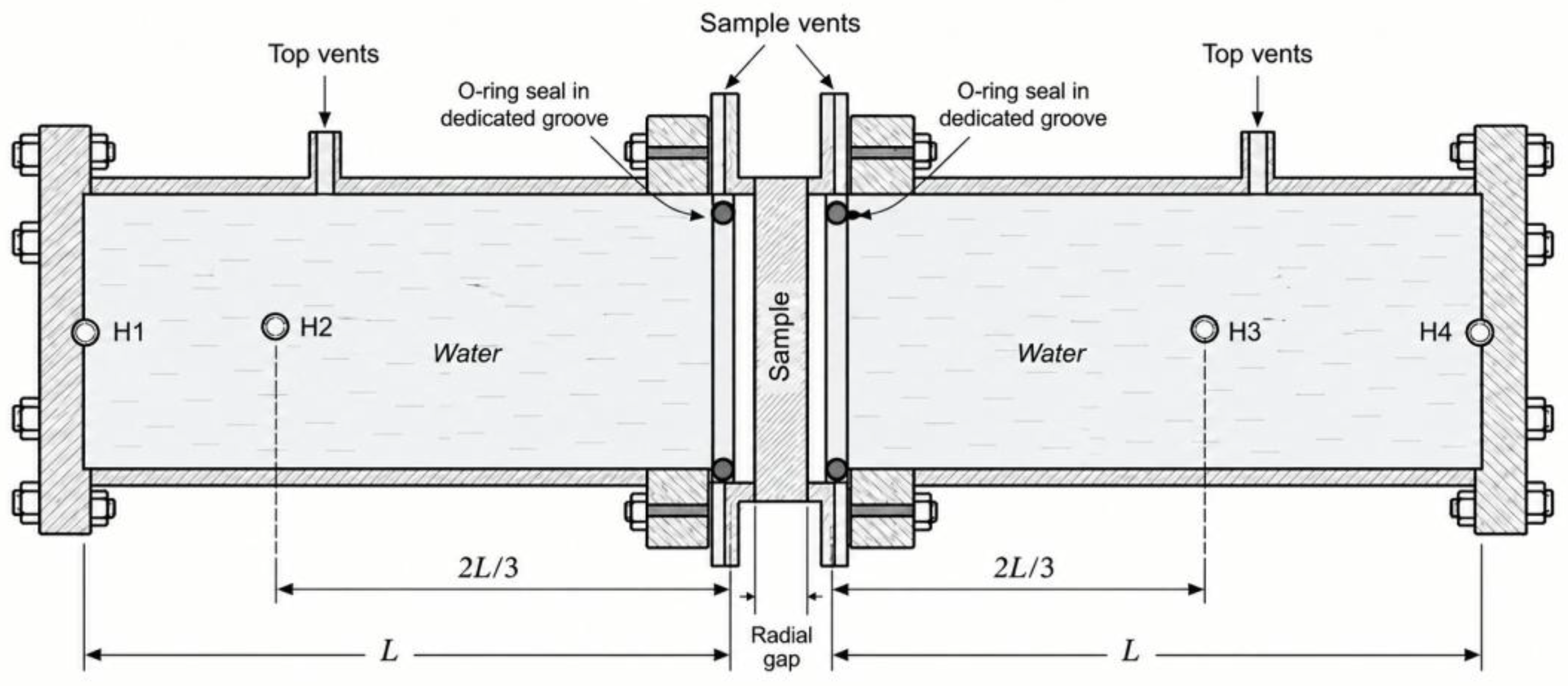
Figure 2.
Normal-incidence R(f), T(f) and α(f) for POM layer in the water.
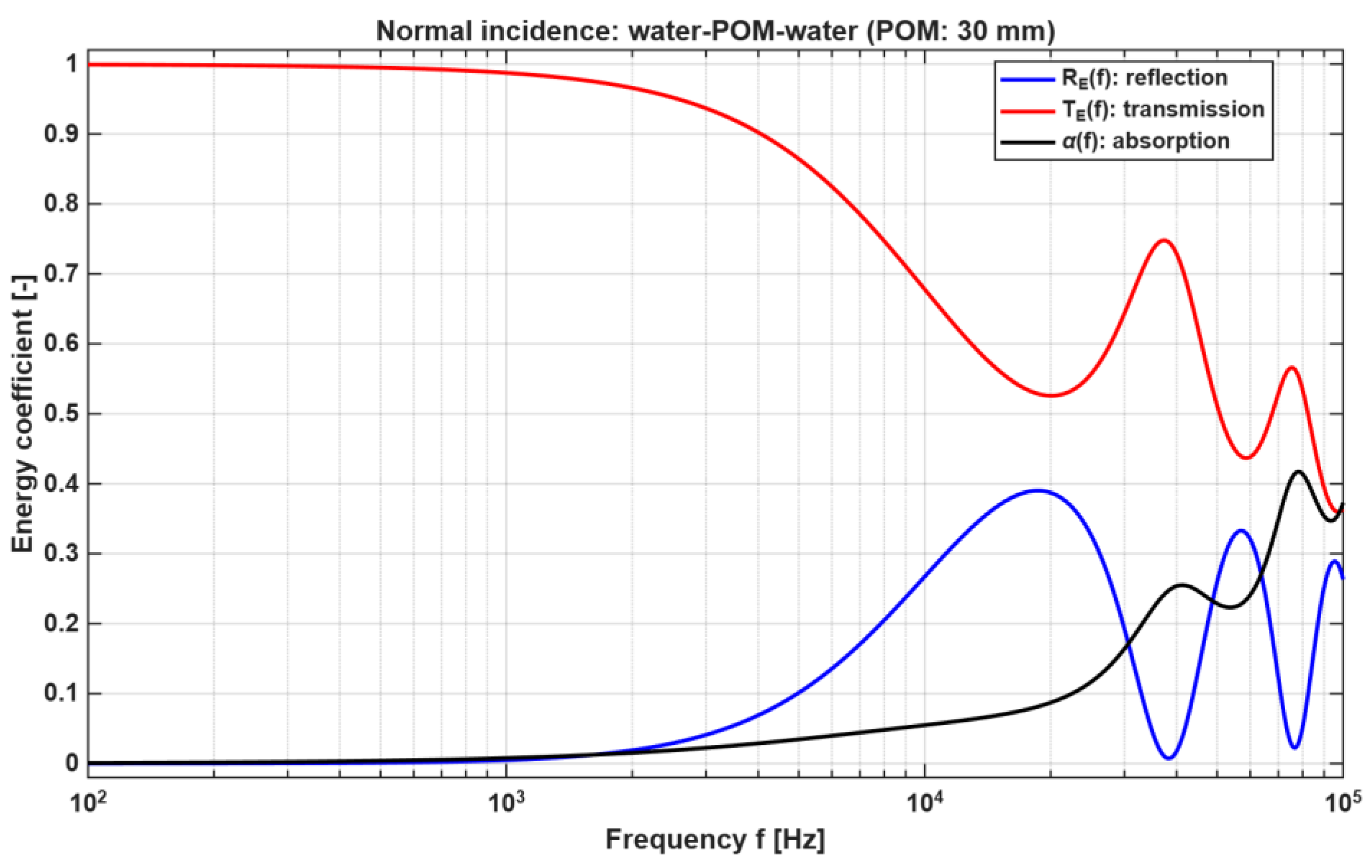
Figure 3.
Normal-incidence R(f), T(f) and α(f) for two layer system in water.
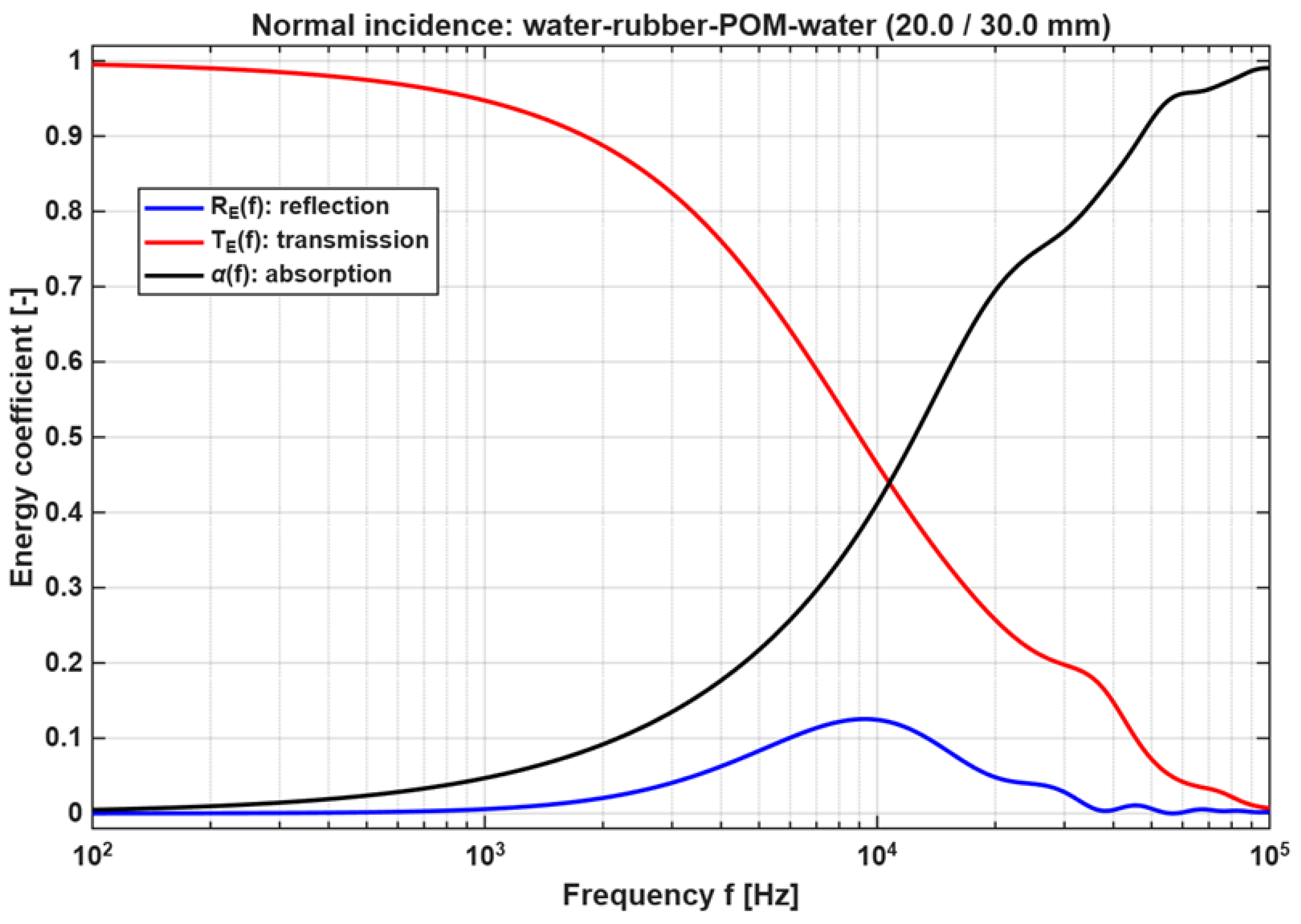
Figure 4.
Absorption coefficient vs frequency (log Y).
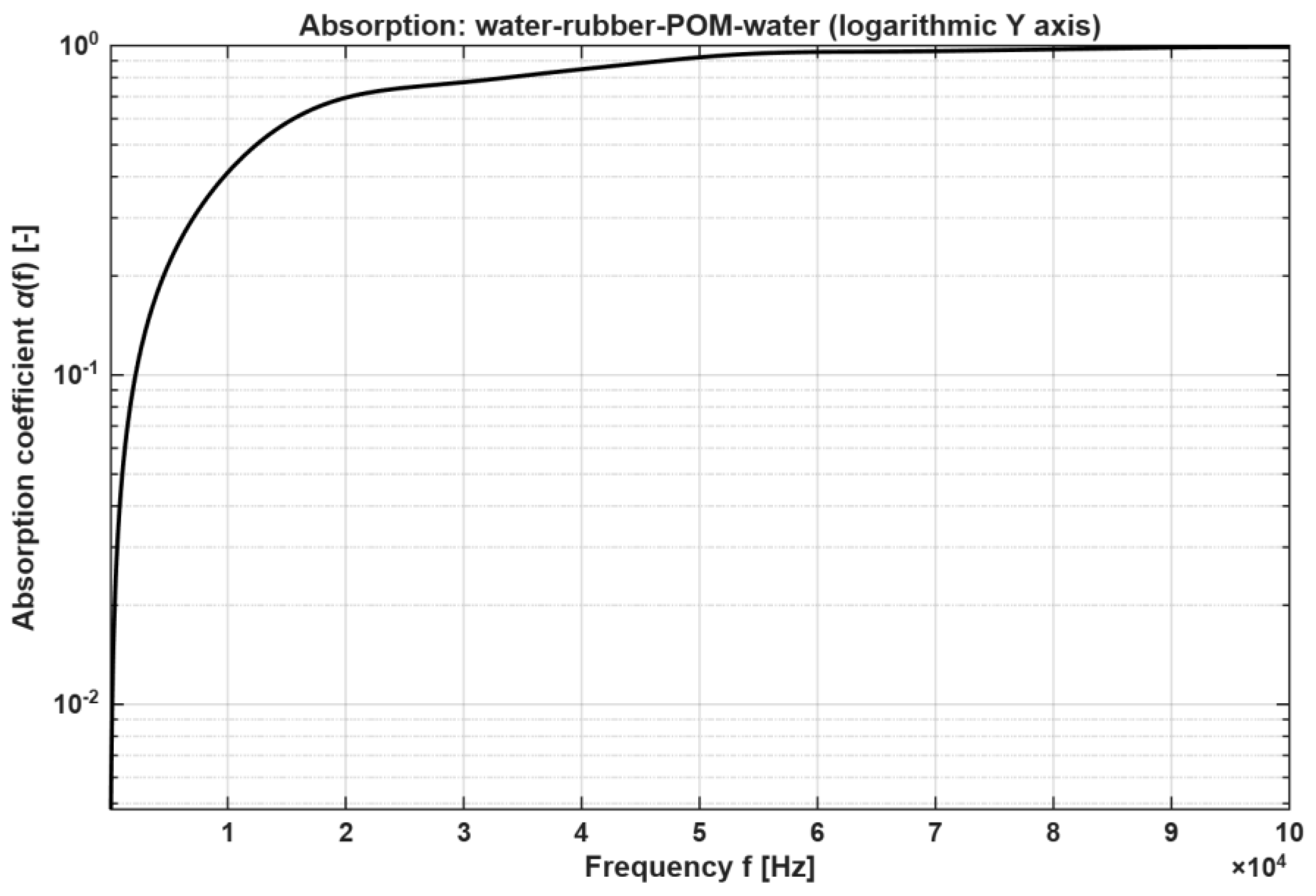
Figure 5.
The first water-filled impedance tube stand: (a) general view. (b) sample and top vent valves view.
Figure 5.
The first water-filled impedance tube stand: (a) general view. (b) sample and top vent valves view.
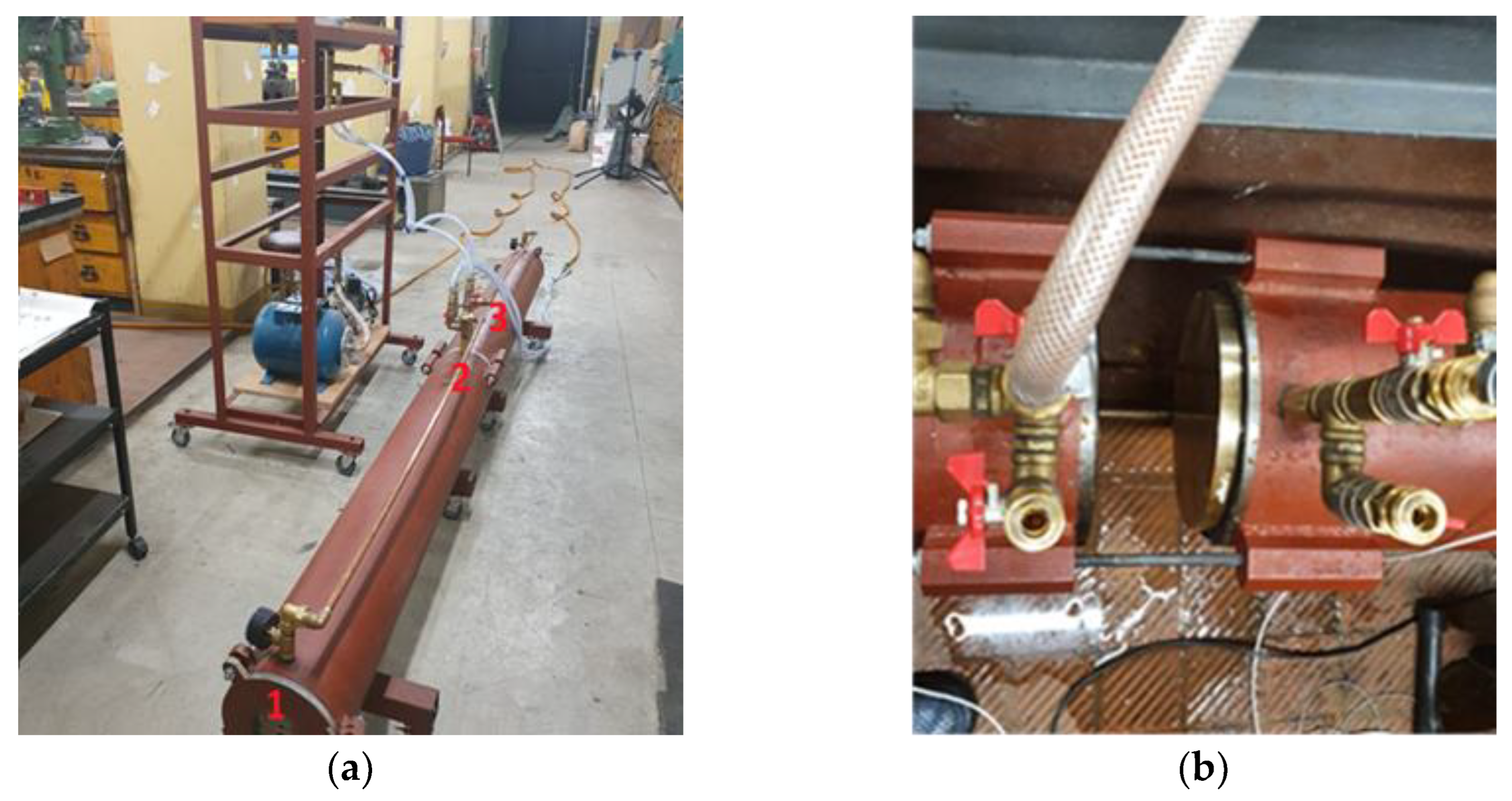

Table 1.
Preferred material by frequency for water-filled impedance tubes.
| Frequency family | Recommended tube material | Reasoning |
| Up to 1 kHz | Carbon steel or stainless steel 316L | Very large diameter and high water mass demand maximum stiffness. Corrosion resistance favours 316L, cost favours carbon steel with internal protection. |
| From 1 kHz to 10 kHz | Stainless steel 316L | Best overall compromise between stiffness, corrosion resistance, machinability, and long-term laboratory durability. |
| Over 10 kHz | Stainless steel 316L | Small geometry benefits from dimensional stability, corrosion resistance, and precision micro-machining; aluminium is less favourable because lower stiffness increases sensitivity to wall compliance. |
Disclaimer/Publisher’s Note: The statements, opinions and data contained in all publications are solely those of the individual author(s) and contributor(s) and not of MDPI and/or the editor(s). MDPI and/or the editor(s) disclaim responsibility for any injury to people or property resulting from any ideas, methods, instructions or products referred to in the content. |
© 2026 by the authors. Licensee MDPI, Basel, Switzerland. This article is an open access article distributed under the terms and conditions of the Creative Commons Attribution (CC BY) license (http://creativecommons.org/licenses/by/4.0/).
Copyright: This open access article is published under a Creative Commons CC BY 4.0 license, which permit the free download, distribution, and reuse, provided that the author and preprint are cited in any reuse.