

Submitted:
20 October 2026
Posted:
21 October 2026
You are already at the latest version
Abstract
Pressure-driven tube flow links a fluid’s flow curve to its velocity profile and throughput, and underlies velocimetric rheometry. We formulate them through the complementary dissipation potential, the Legendre–Fenchel conjugate of the dissipation potential, whose stress derivative is the inverse flow curve. Flat intervals and corners of the potential locate plugs and shear-rate jumps, an integrability criterion decides whether a finite velocity profile exists at a limiting constitutive stress, and the cross-sectional integral generates the pressure–flow curve and recovers the pressure-work balance. For velocimetry, velocity differences give exact mean shear rates over specified stress intervals, and monotonicity bounds the rate at every interior sample stress. Finite samples, however, give no general upper bound on the wall shear rate. Declaring an upper bound on the logarithmic slope of the inverse flow curve yields an explicit two-sided wall shear-rate bracket; a simultaneous Gaussian multiplier retains its conditional coverage when the width is chosen from finite candidates using the data. In synthetic Newtonian, Bingham, Herschel–Bulkley and Carreau–Yasuda ensembles at 1% velocity noise, median potential errors are 0.44–0.60%, whereas regularized wall shear rates have median biases of −7% to −12%. On the same profiles, the 90th-percentile wall shear-rate error is 5.1–6.9% for bracket midpoints with valid fluid-specific slope bounds, against 10.1–15.3% for regularized estimates, a gain that reflects the added constitutive information. Velocity-drop, stress-calibration and near-yield scalings give criteria for the attainable stress resolution and plug detectability.
Keywords:
complementary dissipation potential
; Legendre–Fenchel transform
; yield-stress fluids
; capillary flow
; velocimetry
; pressure–flow relation
1. Introduction
Pressure-driven capillary flow connects two practical questions. Given the flow curve of a fluid, what velocity and throughput will a pressure gradient produce? Given a measured velocity profile, what can be inferred about the flow curve? Both questions arise in pumping, polymer processing and rheometry [1,2,3]. For fully developed flow in a circular tube, momentum balance determines the shear stress independently of the material. The remaining calculation, or inference, concerns the constitutive response over that stress range.
The classical capillary stress integrals express the flow rate through the inverse relation between stress and shear rate [4,5]. Analytical solutions are available for several important laws, including Ellis, Carreau, Cross and Carreau–Yasuda [6,7,8]. Changing the independent variable can simplify their evaluation [9,10]; a hypergeometric framework develops this approach for Carreau–Yasuda profiles and flow moments [11]. These formulations supply the velocity and throughput, but the relations between different constitutive features and the information contained in a measured profile are also of interest.
The complementary dissipation potential makes these relations explicit. It accumulates the inverse flow curve along the stress axis, so its derivative is the shear rate. Wang et al. [12] used this potential to express the tube velocity as a difference of two potential values. The same function is the stress-rescaled velocity introduced for capillary velocimetry by Tozzi et al. [13]. The area interpretation and virtual-tube constructions of Tozzi and Hartt [10] and Kim [9], corrected in Kim [14], contain related information. Thus the potential used for a forward calculation is also a constitutive quantity accessible from velocity measurements.
This description belongs to established convex and complementary formulations of viscous flow [15,16,17,18,19]. In particular, Kamrin and Goddard [20] connect local dissipation potentials to global flow potentials, including nonlinear boundary slip. Their theory gives the mean velocity as a pressure-gradient derivative. In a circular tube, the known stress field allows an explicit cross-sectional realization of this principle. No additional spatial variational problem is needed to construct the capillary potential.
Here we develop three applications of . Its values and geometry first connect constitutive features to velocity profiles and give an integrability criterion for a finite profile at a limiting stress. Its cross-sectional integral then supplies an explicit capillary potential for the pressure–flow response and pressure-work balance. Finally, its secants identify exactly which constitutive averages are measured by finite velocity differences. We establish the different information available for interior and wall rates, derive a wall-rate bracket from a declared upper logarithmic slope, and quantify the roles of velocity noise, pressure calibration and the near-yield flow law. Carreau–Yasuda and Herschel–Bulkley profiles illustrate the forward applications; synthetic ensembles for four rheologies assess the measurement results. The established velocity representation and global potential principle provide the framework for these applications and resolution results.
2. Complementary Potential and Capillary Velocity
2.1. Tube Flow and Stress Distribution
We consider steady, laminar, isothermal flow of an incompressible fluid in a straight circular tube of radius R. The flow is fully developed and driven by a pressure drop per unit axial length . Let r be the radial distance from the tube axis and the axial velocity. The shear-rate magnitude is
and the positive shear-stress magnitude satisfies
Symmetry and regularity at give
Here is the radial stress gradient and is the wall shear stress. The stress distribution is independent of the constitutive model. We impose no slip at a stationary wall, , except in Section 5.9. The volumetric flow rate is .
We assume that the local steady shear-stress relation is monotone and that the material properties are independent of pressure and position. Temperature variations, evolving thixotropic structure and flow instabilities are excluded. The fully developed assumption requires a sufficient distance from the entrance, which can be substantial for non-Newtonian fluids [21]. A steady shear-stress function can also be used for a viscoelastic material when a stable rectilinear viscometric flow exists [22]; elastic transients and secondary motion are outside the present description.
2.2. Constitutive Potentials and Admissible Flow Curves
Let be a continuous, nondecreasing stress for . Its zero-rate limit is the ideal yield stress, ; stresses can be sustained at zero rate. A fluid without a yield stress has . The upper stress limit is . We initially require ; the endpoint case is treated in Section 3.2.
Write the inverse flow curve as , choosing for . Its stress integral defines the complementary potential:
The first potential accumulates stress along the rate axis; the second accumulates rate along the stress axis. The supremum is the Legendre–Fenchel transform of the convex function [15,23]. Both potentials have units of power per unit volume. Their relation to the physical dissipation rate is developed in Section 3.3.
Figure 1 connects the maximization in panel (a), the complementary areas in panel (b) and the velocity-producing strip in panel (c). In panel (a), the largest vertical gap between the line and is . For a smooth flow curve, the maximum occurs where . Below an ideal yield stress, the maximum occurs at and is zero.
The derivatives recover the same constitutive relation in either variable:
The second equality holds almost everywhere when the inverse curve has jumps. At a plateau stress, any rate within the corresponding plateau interval can be assigned to at that stress. Since takes the value at one radius only, the choice does not alter a velocity integral. The left and right slopes of give the rates on either side. For a Newtonian fluid, and .
Monotonicity must be checked for each input law. For a differentiable viscosity, the condition is . With and positive time and transition parameters, the Carreau–Yasuda examples with and Cross examples with satisfy it. For Cross exponents , it additionally requires .
2.3. Velocity from the Potential
Integrating with gives
The definition of then gives the established representation [12]
Whenever is finite, it determines a unique no-slip profile whose rate satisfies the constitutive relation almost everywhere. Since , the centreline velocity is
Equation (8) is useful because one constitutive function supplies every point of the profile. After has been evaluated over the relevant stresses, changes in tube radius or pressure gradient enter through and . For a Newtonian reference, gives . For a yield-stress fluid, a flat part of gives a uniform velocity. The representation collects the classical stress integral and the area construction of Tozzi and Hartt [10] in the same constitutive function used below for velocimetry.
2.4. Evaluating the Potential
The potential can be evaluated from either form of the flow curve. If is available, use its stress integral in (). If stress is specified as , the constitutive relation instead gives
For a prescribed pressure gradient, determine the wall rate from . The profile then follows parametrically:
This is the shear-rate parametrization of Wang [8] expressed through the complementary potential. It requires constitutive inversion at the wall, but no further inversion to generate the parametric curve. Evaluation on a prescribed radial grid may subsequently require interpolation or local root finding.
For a fluid without yield stress, . For an ideal yield-stress fluid, the limit locates the plug edge and (8) supplies the uniform core velocity. The integral defining can be evaluated analytically or by quadrature. Carreau–Yasuda and Cross expressions can be written using hypergeometric functions [8,12]. Table 1 collects the potentials used below. The Newtonian and Herschel–Bulkley entries give direct profile formulas, whereas the Carreau–Yasuda entry specifies parametric evaluation. The two saturating laws provide contrasting tests of the limiting-stress criterion in Section 3.2.
3. Velocity Profiles and Constitutive Limits
3.1. Yield Stress and Stress Plateaus
The slope of the potential gives the local rate, while a potential difference gives the velocity. Their combination lets constitutive features be read directly as features of a tube profile. Figure 2(a) contrasts a flat potential interval and a corner with a Newtonian reference; panel (b) shows the corresponding plug and velocity kink.
An ideal yield stress gives
The velocity is consequently uniform where . For , the plug radius and velocity are
For , the no-slip flow has . In Figure 2, the Bingham flat interval ends at in panel (a), giving the plug of radius in panel (b) at .
The potential also shows how adding a yield stress changes a base-fluid profile. Let have zero yield stress and potential . Replacing its flowing branch by gives
The constitutive change translates the stress argument and introduces the flat interval responsible for the plug. A Newtonian base gives Bingham flow; a power-law base gives Herschel–Bulkley flow. Substitution into (8) supplies both the core and the sheared profile without separate integrations. The Herschel–Bulkley potential was also obtained as a stress-rescaled velocity by Tozzi et al. [13]. Papanastasiou regularization instead gives a positive rate at every positive stress, so it approximates a plug without an exact flat interval [24,25].
A stress plateau has the complementary signature. If for , the inverse curve jumps at and has a corner. For , the velocity is continuous but its slope changes at , from to . The corner at in Figure 2(a) therefore produces the kink at in panel (b), without a plug. Kinked profiles have been observed in micellar systems [26]. Here the plateau is prescribed as part of the steady flow curve; a local monotone law does not select its stress, interfacial thickness or dynamics [27].
3.2. Limiting Constitutive Stress
Some empirical flow curves approach, without attaining, a finite stress as shear rate increases. For these laws a finite wall shear rate requires , or . Above that stress the constitutive model cannot support the imposed loading. For the complementary potential is infinite and the inverse constitutive relation is undefined. A stress field that exceeds this limit over part of the cross-section therefore has no solution within the assumed steady constitutive model.
At the limiting wall stress , a finite velocity profile requires
The second integral gives the same condition directly from the flow curve: the remaining stress difference must be integrable over shear rate. For a law that approaches its limiting stress only as , the wall shear rate is then unbounded even when the velocity remains finite. This is a singular limiting profile. If the terminal stress is attained on a plateau at finite shear rate, a finite wall shear rate can instead be chosen.
The Cross law and the saturating Carreau law both approach . Their potentials, listed in Table 1, behave differently at this stress. The Cross potential diverges, whereas the Carreau potential reaches the finite value . Only the latter therefore gives a finite-velocity profile at the limiting wall stress. More generally, for the saturating Carreau–Yasuda law with and , the stress difference decays as at large q, so the endpoint potential is finite precisely when . The Cross case has and the Carreau case has . Regular solutions with finite wall shear rate require for both of these asymptotically saturating laws.
3.3. Geometrical Interpretation and Dissipation
The geometrical interpretation is shown in Figure 1(b). On the flow curve, the area under and the area to its left sum to the rectangle , giving
This is the equality case of the Fenchel–Young inequality [15,28]. In Figure 1(c), the horizontal strip between local stress and wall stress has area . Moving inward through stresses below yield adds only strips of zero width, so the velocity stops changing and a plug appears. This area reading of the velocity is consistent with Tozzi and Hartt [10]; the potential records the accumulated area as a function of stress.
The local physical dissipation rate is . Equation (16) partitions this rate into two constitutive potentials; the individual terms do not represent separate loss mechanisms or stored energies. For a Newtonian fluid they are equal, on the flow curve. For , they satisfy . For the Bingham law, while on the yielded branch. Thus the relation between either potential and the physical dissipation depends on the constitutive law.
3.4. Illustrative Velocity Profiles
Figure 3 illustrates the connection between complementary potentials and tube velocity profiles for Carreau–Yasuda and Herschel–Bulkley fluids. All quantities are nondimensional, with a unit tube radius.
For the Carreau–Yasuda law,
we take , , , , and . The decrease in viscosity increases the shear rate near the wall, where most of the velocity variation occurs. The blunt core in Figure 3(c) corresponds to the rapid increase of at high stress in panel (a).
For the Herschel–Bulkley law, take , , and . Substituting its potential from Table 1 into (8) gives Figure 3(b,d): vanishes for and the velocity is uniform for . The plug velocity is . The flat potential interval and uniform core are the same constitutive feature expressed in stress and radial coordinates. The additional curves in panel (c) are the comparison bounds derived in Section 3.5. In all four panels, the potential-based curves agree with the independent integration of , checking both the recovered potential and the predicted profile.
3.5. Bounds from Constitutive Order and Convexity
Constitutive order and convexity constrain a profile even when the full potential has not been evaluated. Consider two fluids in the same tube at a fixed pressure gradient. If for all , then (7) gives everywhere and . In particular, at all relevant shear rates implies this ordering. Comparing only the endpoint values and is insufficient to order the entire profiles: the shear-rate ordering over the stress interval is what controls the result.
For a shear-thinning fluid with no yield stress and a finite zero-shear viscosity , let be the viscosity at the wall. If viscosity is nonincreasing with shear rate, then for . Substitution in (7) gives the bounds
The wall-viscosity upper bound is useful when is measured or after it has been calculated; it is not an a priori estimate from alone.
Two additional bounds hold for any monotone flow curve with finite wall shear rate. Convexity places below its chord from 0 to and above a supporting line at . In velocity form these give
At a wall stress that coincides with a plateau, the upper bound uses an admissible supporting slope of there. The bounds follow from the concavity of u, since its slope is nonincreasing. Figure 3(c) shows that the Carreau–Yasuda profile lies above its centreline-to-wall chord and below the supporting wall tangent, as well as between the two Newtonian profiles. These comparisons provide consistency checks for numerical solutions and measured profiles, subject to experimental resolution and noise.
4. Pressure–Flow Response and Dissipation
The potential determines throughput as well as the profile. Its cross-sectional integral also supplies a pressure-controlled capillary potential. We use these relations to connect local rheology, global loading and the physical pressure-work balance.
4.1. Flow Rate from the Constitutive Potential
Substituting (8) into and using gives
Thus the same function used for point velocities determines the complete pressure–flow curve as varies. The radial weighting is retained explicitly; a flat potential interval contributes a moving plug when the outer material is yielded. If , both potential values vanish and the no-slip flow rate is zero.
4.2. Integrated Complementary Potential
To describe the response of the whole capillary at an imposed pressure gradient, we integrate the local complementary potential over the cross-section,
This quantity has units of power per unit axial length. Differentiating at an admissible interior load, using , yields
The last equality follows by integration by parts in . Equation (23) relates the flow rate to the sensitivity of the integrated potential to the imposed pressure gradient. It is the global counterpart of and is consistent with classical complementary principles for nonlinear viscous flow [17,18,19]. More specifically, Kamrin and Goddard [20] connect the pressure gradient and mean velocity through a global potential, including dissipative wall slip. Equation (23) realizes the scalar capillary case through the explicit cross-sectional integral in (22). The known stress field therefore supplies the global potential by direct integration of the constitutive potential.
Because is convex and stress is linear in G, is convex. Consequently is nondecreasing wherever the stated solution exists. For an ideal yield-stress fluid, for . The flat interval in the local potential therefore becomes a threshold in the global loading response.
Figure 4 illustrates this connection for the Herschel–Bulkley fluid used in Figure 3, now with a variable pressure gradient. The capillary potential is flat up to . Above this threshold it becomes progressively steeper, and its slope gives the increasing flow rate. At the marked operating load, the tangent in panel (a) supplies the throughput shown in panel (b). Thus one integrated constitutive function describes both the onset of flow and the pressure–flow response.
The physical pressure work is obtained from the momentum equation and the no-slip boundary condition:
This is a power balance per unit axial length. It is the cross-sectional integral of (16). If the steady flow rate is taken as the imposed quantity, the corresponding global dissipation potential is
Here the supremum is over nonnegative loads with finite , including finite limiting values at stress-domain endpoints. For the actual no-slip flow at an admissible interior load, (23) identifies G as a maximizing load and gives
Thus form a conjugate pair for the capillary, corresponding to the local pair . The potentials and describe pressure-controlled and flow-controlled operation, respectively. In ideal yield-stress flow, over a finite range of pressure gradients; the global relation is then understood in the same subgradient sense as the local law.
5. Constitutive Information from Capillary Velocimetry
For a forward calculation, determines u. For rheometry, the same relation can be read in reverse: a measured velocity difference determines a potential difference. This identifies the constitutive quantity available before differentiation and suggests reporting finite stress-interval averages when local slopes are poorly resolved. We examine what this offers for noisy profiles, including the distinct requirements for wall rates and plug-edge location.
5.1. What Velocity Differences Measure
Rearranging (8) gives
A velocity profile measured together with a fully developed pressure gradient therefore determines the potential over the sampled stress range. This is the stress-rescaled velocity function of Tozzi et al. [13]. Ultrasound and NMR velocimetry provide the required spatial information [29,30,31,32]. The construction does not require a selected constitutive model. Recovering the pointwise shear-rate curve still requires differentiation or an equivalent regularized inverse calculation.
A finite velocity difference has a more direct constitutive interpretation. For and , , it gives the shear rate averaged uniformly over that stress interval:
The common centreline reference cancels. This average is a resolved constitutive quantity in its own right. Assigning it to a point introduces an averaging bias that depends on the curvature of the inverse flow curve.
If the two velocities have independent errors with standard deviation , the direct average in (28) has standard deviation . A Gaussian uncertainty multiplier z and relative half-width therefore require, for planning purposes, a velocity drop of at least . If one endpoint is the exactly known no-slip wall velocity, is replaced by . Wider intervals improve the signal relative to noise while averaging over more of the constitutive curve. Their stress width should be reported with the inferred rate. Correlated velocity errors require the covariance of the two measurements in place of the independent-error expression.
For a smooth positive branch, this averaging bias can be quantified. Let a centred interval of stress width estimate the rate at its midpoint . Taylor expansion of (28) gives bias , while independent endpoint noise gives variance . When , minimizing the leading mean-square error gives
This is a local planning relation: the interval must stay on the smooth branch and within the measured stress range. A wider interval suppresses noise but averages over more constitutive curvature. For the baseline Herschel–Bulkley law, on the yielded branch; at 1% velocity noise, (29) gives , about nine of the 40 radial sampling intervals. The interval average itself has no point-assignment bias.
Monotonicity also distinguishes interior rates from endpoint rates. Whenever both neighbouring intervals are available, it gives
For velocities known within absolute errors , the corresponding lower and upper bounds are widened by the sums of the endpoint errors divided by h. At the wall there is no outer interval. Monotonicity supplies a lower bound from an inner secant, but no general finite upper bound on the point wall rate from finitely sampled velocities alone. This remains an identifiability issue even for exact samples. To see it constructively, let be the penultimate sample stress, and s the mean rate in the last interval, with . For any , replace the inverse curve on that interval by
It is continuous, nondecreasing and has the same interval average s, so all sampled velocities are unchanged although its wall rate is M. This construction applies to a continuous curve increasing on the last interval; an exactly constant interval is a degenerate case. The difference between the associated flow rates is at most , because the profiles differ only within that annulus. Thus a well-constrained integral can coexist with an unbounded endpoint derivative. A finite two-sided wall-rate estimate requires information on how rapidly the unresolved rate is allowed to grow.
Integrated flow quantities remain accessible before recovering a local derivative. Subtracting from a measured profile gives the profile in a smaller virtual tube of radius ℓ at the same G; its flow rate can then be integrated directly. This construction underlies Tozzi and Hartt [10] and is related to the method of Kim [9]. It helps explain why useful pressure–flow information can remain available when local rheological detail is poorly resolved.
5.2. A Wall-Rate Bracket from a Declared Constitutive Slope
The additional information can be expressed as a bound on the relative growth of the inverse flow curve. On a positive, absolutely continuous branch, write
Suppose is specified over the outer interval , where . Integrating this bound from to the wall gives . Averaging and using monotonicity then yields the explicit bracket
where . The lower bound is approached by nearly constant rates, and the upper bound is attained by a rate proportional to . The fractional gap satisfies . For the Herschel–Bulkley example, and give when the endpoints are exact, with the numerical endpoints expressed relative to the generating wall rate.
With an exact no-slip wall velocity and one Gaussian-noisy inner velocity, the measured secant has standard deviation . A bracket with coverage at least is
where is the standard normal distribution function. On the event , both endpoints bound the true rate by (33); a negative upper endpoint produces an empty bracket and lies outside that event. A larger interval lowers noise but widens the constitutive bracket. If the width is selected from K candidates using the same data, replacing z by gives simultaneous coverage at least , by the union bound. Any selection among those brackets retains this coverage; independence between candidate secants is unnecessary.
The upper slope bound is additional constitutive information and must be declared with the result. For a power-law index , suffices. For Herschel–Bulkley flow, , so the interval must lie above yield. A bound inferred from the same noisy profile requires its own uncertainty assessment. Coverage in (34) is conditional on a valid bound, known Gaussian noise, accurate positions and calibrated stress.
5.3. Synthetic Profiles and Reconstruction
We use the nondimensional Herschel–Bulkley case in Figure 3, with , , , and . The exact profile is sampled at 41 equally spaced radial positions, including the axis and wall. Independent Gaussian noise is added to each velocity:
Here . The pressure gradient and sample positions are initially taken as exact, and spatial averaging is omitted. All measurements are synthetic.
For , the potential differences have errors
Their standard deviation is , and they are correlated through the centreline measurement. An interior central difference of instead has noise standard deviation , with . These values are 1.4% of the wall potential and 6.3% of the wall rate, respectively. The potential can therefore retain useful information while raw derivative estimates fluctuate; these normalized noise levels concern different targets.
To illustrate regularized recovery, we fit the original noisy velocities directly, retaining the exact no-slip condition. We represent by a piecewise-linear, nonnegative, nondecreasing function on 20 equal stress intervals, with , and minimize
Nonnegative nodal increments enforce the shape constraints. The generating law and yield stress are not supplied to the fit. In Figure 5, the weight is selected by matching the root-mean-square velocity residual to the known noise standard deviation, following the discrepancy principle [33], then held fixed for 200 further independent noise realizations.
This is an established type of regularized inverse problem [33,34]; model-based velocimetry inference also recovers constitutive parameters and their uncertainties [35]. Since , the penalty in (37) equals . The estimator is therefore equivalent to a smooth, decreasing, concave velocity-profile fit with the same representation and boundary conditions. The potential gives these constraints a constitutive interpretation, allowing the same fit to be assessed as a potential, interval-average response and pointwise flow curve.
Figure 5(a) shows that the fitted velocity closely follows the generating profile, and panel (b) shows the corresponding agreement in potential. Panel (c) exposes the greater scatter of raw velocity derivatives and the regularized fit’s low wall-rate estimate. The shaded ranges quantify variability across repeated noise realizations at the fixed weight; their small spread in panels (a,b) does not imply equally accurate local rates in panel (c).
We also use a Newtonian fluid with , a Bingham fluid with , , and the Carreau–Yasuda fluid in Figure 3. Here and , except for the Carreau–Yasuda case, where . Baseline sampling uses points, stress intervals and . In these extended ensembles, the discrepancy weight is reselected for every noisy profile, except in the explicit penalty sweep. If the minimum shape-constrained residual is already at least the prescribed noise level, we retain . Each noisy condition has 200 independent realizations; noiseless conditions use one deterministic fit. Common Gaussian draws on nested radial positions pair comparable conditions. The study contains 46 reconstruction settings and 8006 fits, with five calibration settings evaluated from the baseline profiles. Conditions and individual results are included in the reproducibility data.
To distinguish integrated and local reconstruction errors, we define
We also use and . The true yield stress enters assessment only. These wall-normalized averages avoid division by zero, but does not assess leakage within the plug or the relative accuracy of small local rates. Table 2 shows median potential errors of 0.44–0.60%, yielded-branch rate errors of 1.79–2.25% and flow-rate errors below 0.6%, alongside median wall-rate biases of approximately % to %. All percentile ranges describe variation under the prescribed simulation assumptions and do not correct regularization bias.
5.4. Stress Intervals Resolved by the Synthetic Profiles
To assess local constitutive information, we now use the interval average in (28) as the target. We divide the stress range into reporting intervals of width . For each interval, we compute the absolute relative error in its reconstructed average over the 200 realizations. An interval passes an illustrative resolution criterion when the 90th percentile of this error is at most 10%. We assess whole intervals on the true yielded branch; zero-rate and yield-crossing intervals are treated separately in the plug discussion. The threshold and reporting width specify the measurement question, rather than an intrinsic boundary between recoverable and unrecoverable rheology.
Figure 6(a) compares the four fluids at 1% velocity noise, while panel (b) varies the noise for Herschel–Bulkley flow. Table 3 lists the passing stress ranges and compares the final interval average with the point wall rate. At 1% velocity noise, the passing intervals cover for the Newtonian fluid, for Bingham, for Carreau–Yasuda and for Herschel–Bulkley. These ranges refer to averages over the stated intervals, not to every point within them. Small low-stress rates are harder to recover in relative terms even when their absolute error contributes little to . Filled symbols in Figure 6(a,b) identify the passing intervals; open symbols identify those above the error criterion.
In Figure 6(b), reducing the velocity noise to 0.25% extends the Herschel–Bulkley passing range to . At 5% noise only the interval passes. The latter profile therefore does not resolve the yielded flow curve at this precision and interval width, although integrated quantities can remain useful.
The final interval is also distinct from the point wall rate. At 1% noise, the Herschel–Bulkley average over has a 90th-percentile error of 8.6%, compared with 13.9% for the point wall rate. For Carreau–Yasuda these errors are 9.6% and 15.3%. Reporting a finite-interval average is therefore better supported by these profiles than assigning the same precision to the wall derivative.
The ranges depend on the estimator, constitutive curve, reporting width and known-noise assumption. They cannot be assigned to experimental data without additional uncertainty assessment. For measurement design, (28) first specifies the desired stress width and its velocity-drop signal. The reconstruction then supplies a conditional estimate at that resolution. A broad interval should not be labelled a pointwise rheogram, and an accurate potential should not be used as evidence that all of its local slopes are accurate.
5.5. Wall-Rate Sensitivity to Regularization and Coverage
The endpoint limitation in (30) explains why the wall rate is particularly dependent on regularization. Figure 7(a) uses fixed multiples of the weight selected in Figure 5 to isolate penalty sensitivity, whereas panel (b) and the other extended ensembles reselect the discrepancy weight for each noisy profile. In panel (a), multipliers , and 10 give median wall-rate biases of approximately %, % and %. The unpenalized fit has little median bias but a broad noise range; stronger regularization narrows that range while introducing a negative endpoint bias. The known reference is used to assess these effects, not to select a weight for measured data. Matching the velocity residual to the noise level controls data agreement, but does not guarantee an unbiased endpoint derivative.
Removing outer velocity samples has a similar consequence. Figure 7(b) retains the exact no-slip wall velocity while removing measurements beyond , or . At , the median wall-rate bias is approximately %, compared with % for full coverage. Median rises from 2.25% to 5.07% and from 0.35% to 1.63%. These errors include the unmeasured annulus. The known wall velocity constrains its integrated rate, but supplies no missing local gradient measurement.
Refining the inverse representation cannot replace missing observations. In the archived tests at and 1% noise, increasing the stress-grid resolution beyond did not materially improve rate accuracy. Additional independent samples provided a modest improvement when the per-sample noise was held fixed. These comparisons omit acquisition-time constraints and spatially correlated instrument errors.
5.6. Assessment of the Wall-Rate Bracket
We apply (34) to the archived observations and exact wall velocity. The eight widths use outer sampling intervals, so . We select the smallest relative bracket width with the simultaneous multiplier . Each is the maximum generating-law slope over the outer 20% of the stress range, rounded upward to a multiple of 0.25. The generating law supplies this correct external bound and assesses errors; it remains absent from the regularized fit.
Table 4 gives 90th-percentile midpoint errors of 5.1–6.9%, compared with 10.1–15.3% for the regularized endpoints. All 200 brackets per fluid contain the true wall rate. Their median full widths are 25–31%: the full bracket carries the uncertainty statement. The comparison quantifies the value of the additional slope information. Its tightness matters for the bracket width: the common valid bound widens every bracket, to a median of 52.4% for the Newtonian fluid. It also raises the midpoint error to 17.1% for the Newtonian fluid, above the 10.1% regularized error, and to 10.1% for the Bingham fluid, whereas the Herschel–Bulkley and Carreau–Yasuda midpoint errors (5.8% and 5.7%) are no larger than with the fluid-specific bounds. Results for this common bound, additional noise levels and individual brackets are archived.
5.7. Stress Calibration
Pressure calibration introduces a different uncertainty. If the gradient used to assign stress is , an exact profile gives
On a smooth positive branch, the rate error at a fixed true stress is thus
The same logarithmic slope that bounds wall-rate extrapolation therefore amplifies stress-calibration errors. For Herschel–Bulkley flow, . It increases towards yield, where small stress shifts produce large relative changes in rate. The linear approximation requires both stresses to remain on that positive branch. At the baseline stress , . Allocating a 10% relative-rate error to calibration alone therefore requires approximately % in the linear approximation. The exact shifts for % and % are approximately % and %, as shown in Figure 8(a). The reconstructed curve also contains the baseline error from fitting the noisy velocities, including its nonzero bias at zero calibration error. A pressure-scale error cannot be inferred from a velocity profile alone when the constitutive law is also unknown.
5.8. Plug Resolution and the Velocity-Noise Floor
The near-yield flow law determines the velocity signal available for plug identification. If as , with , integration from to , where is the radial distance into the yielded region, gives
Thus the two-point detection distance decreases only as . The inverse curve becomes relatively sensitive to stress near yield, while its integrated velocity signal remains small. For the Herschel–Bulkley law, and these relations become exact. For , the profile gives
Here is the radial distance at which the profile drop equals , the uncertainty threshold for a pair of independent velocity measurements. It is a planning scale for a two-point comparison, not a confidence interval for the fitted plug edge. Pooling measurements or imposing a constitutive model changes the inference; sample spacing and spatial averaging impose further limits.
For , the profile drop grows as , making the first departure from the plug difficult to distinguish. At the baseline 1% noise and , (43) gives , approximately 30% of the sheared radial width. A small potential error can therefore coexist with a poorly located transition from zero to a small positive shear rate. A completely unyielded no-slip profile only gives ; it cannot identify uniquely.
Figure 8(b) varies at fixed , and . Holding fixed reduces the absolute noise as the plug grows and keeps fixed. With the fixed noise floor , the scale instead remains approximately for this fixed-pressure family while the yielded shell shrinks. At , and , so the relative velocity noise reaches 37% and . The total drop across the shell is then below the selected threshold for two independent noisy velocities. Only eight sampled radial intervals remain outside the plug. The ratio therefore gives a direct planning test: as it approaches unity, a two-point comparison cannot distinguish a small departure from the plug within most of the yielded shell. An exactly known wall velocity changes the pair threshold as described in Section 5.1; pooling samples or fitting a material law also changes the inference.
For measurement design, the required constitutive stress interval and acceptable rate uncertainty should be chosen first. The velocity-drop criterion in Section 5.1 then tests whether that interval has sufficient signal. Near-wall coverage is needed when the wall rate is the target; pressure calibration must be tight enough for (41); and a yielded shell must be wide enough and fast enough to distinguish its velocity variation from the noise floor. Reporting the sampled stress range, interval width, velocity uncertainty and dependence on regularization makes the recovered information interpretable. The present simulations quantify these effects for point measurements at exact positions with known independent noise. Applying the planning rules to an instrument requires its spatial response and error covariance.
5.9. Wall Slip and Other Flow Geometries
A prescribed slip velocity adds a constant to the bulk profile,
Velocity differences cancel this constant and still measure the bulk potential. Under slip, however, , not . Figure 9(a) shows the slip-induced translation of the velocity profile at a fixed pressure gradient. Panel (b) shows that centreline-to-local differences recover the same bulk potential for both profiles, separating bulk rheology from the boundary offset. A sub-yield material may slide as a rigid plug, as observed in Carbopol systems [36]. A flat profile then requires the boundary velocity to distinguish sliding from no flow. For a nondecreasing slip law, the boundary potential description of Kamrin and Goddard [20] gives . Adding to (22) restores , since .
The potential difference in (8) relies on the linear stress field. In annular pressure-driven flow, the signed stress is , where follows from the boundary conditions. The nonlinear relation between stress and radius prevents reduction of the velocity integral to a difference of two values. Figure 9(c) compares annular stresses for a Newtonian and a shear-thinning power-law fluid at the same geometry and load. Their different zero-stress radii show how the boundary conditions and flow curve jointly determine the stress mapping. For a noncircular duct, equilibrium constrains two transverse shear-stress components and no longer determines stress independently of the fluid. For an isotropic generalized Newtonian material with no-slip walls, the complementary principle minimizes over stress fields satisfying [20,37,38,39,40]. This is a separate spatial problem [41,42,43]. Figure 9(d) shows an exact Newtonian elliptical-duct example. Its two-component stress field and spatially varying complementary potential density illustrate the quantities needed for this area integral. Bounds on its minimized potential need not bound the derivative Q without additional estimates. Viscoelastic secondary flows introduce further effects outside the scalar framework [44].
Finally, convexity assumes a specified monotone steady flow curve. Taking the conjugate of a nonconvex and then transforming back gives its closed convex envelope [15]; this does not select the physical shear-banding plateau [27]. The present results do not resolve shear-banding dynamics, thixotropy, elastic instabilities or temperature-dependent flow.
6. Conclusions
The complementary dissipation potential gives a single stress-based constitutive function for both forward prediction and inverse inference in fully developed tube flow. Differences of the potential give the velocity, its stress derivative gives the shear rate, and its cross-sectional integral generates the flow rate through differentiation with respect to pressure gradient, recovering the pressure-work balance.
For forward prediction, constitutive features map directly onto profile features: a flat potential interval produces a plug and a corner produces a shear-rate jump. At a limiting constitutive stress, integrability of the remaining stress deficit decides whether the velocity stays finite; for laws that approach the limit only asymptotically, the wall shear rate is then unbounded. For the saturating Carreau–Yasuda law with and , a finite limiting profile exists if and only if ; for the velocity diverges as the wall stress approaches the limit.
For velocimetry, the potential identifies what a sampled profile determines. A finite velocity difference measures the exact mean shear rate over a specified stress interval, and monotonicity bounds the rate at every interior sample stress. The wall shear rate differs in kind: continuous monotone inverse flow curves can reproduce the sampled velocities with arbitrarily large wall shear rates, so finite samples alone provide no general upper bound. A declared upper bound on the logarithmic slope of the inverse flow curve supplies the missing information and yields an explicit two-sided bracket. Under the stated Gaussian measurement model and a valid bound, simultaneous widening preserves its conditional coverage when the bracket width is selected from a finite candidate set using the same data.
The synthetic ensembles quantify the difference between integrated and local information. At 1% velocity noise, median potential errors are 0.44–0.60%, whereas regularized wall shear rates have median biases of % to %. For Herschel–Bulkley flow, the outermost average over a stress interval of width has a 90th-percentile absolute relative error of 8.6%, compared with 13.9% for the regularized point wall shear rate. With valid fluid-specific slope bounds, bracket midpoints have 90th-percentile wall shear-rate errors of 5.1–6.9%, against 10.1–15.3% for regularized endpoints on the same profiles. All 800 baseline brackets contain the true value, with median full widths of 25–31% of it. The gain derives from the additional constitutive information, and the uncertainty is stated by the bracket width rather than by the midpoint error.
These results translate into measurement criteria. The velocity drop across an interval sets its noise budget, the curvature of the inverse flow curve sets the bias of assigning an interval average to a point, and the logarithmic slope sets the sensitivity to pressure-calibration error. Near yield, gives a two-point plug-detection distance that decreases only as . Velocimetric rheology should therefore be reported at a stated stress resolution, together with the noise model and any constitutive information used to infer point or wall shear rates. The analysis assumes monotone, steady flow curves in fully developed circular-tube flow. Uniform wall slip leaves the recovered bulk potential unchanged, whereas annular and noncircular ducts require a separate stress mapping or spatial solution. Applying these criteria to measured profiles, with the instrument’s spatial response and error covariance, is the natural next step.
Funding
This research is funded by the Science Committee of the Ministry of Science and Higher Education of the Republic of Kazakhstan (Grant No. AP26197943).
Author Contributions: Yanwei Wang
Conceptualization, Methodology, Formal analysis, Software, Visualization, Writing – original draft, Writing – review & editing, Funding acquisition.
Data Availability Statement
The Python code, generating parameters and synthetic data supporting this study are openly available at https://github.com/ktwyw/cdp-capillary-velocimetry (release v1.0.0). The repository contains the scripts for all nine figures and four tables, the synthetic velocity samples and noise realizations, every inverse fit, stress-interval assessment and wall-rate bracket, and instructions for regenerating the figures and recomputing the analyses. All velocimetry data in this work are synthetic.
Conflicts of Interest
The author declares no conflicts of interest.
Use of Artificial Intelligence
During the preparation of this work the author used Claude (Anthropic) and ChatGPT (OpenAI) to assist with organizing derivations, preparing analysis and figure scripts, language editing and formatting. After using these tools, the author reviewed and edited the content as needed and takes full responsibility for the content of this preprint. No AI tool is listed as an author.
References
- Bird, R.B.; Armstrong, R.C.; Hassager, O. Dynamics of Polymeric Liquids. In Fluid Mechanics, 2nd ed.; John Wiley & Sons: New York, NY, 1987; Vol. 1. [Google Scholar]
- Bird, R.B.; Stewart, W.E.; Lightfoot, E.N. Transport Phenomena, revised, 2nd ed.; John Wiley & Sons: New York, NY, 2006. [Google Scholar]
- Chhabra, R.P.; Richardson, J.F. Non-Newtonian Flow and Applied Rheology: Engineering Applications, 2nd ed.; Butterworth-Heinemann: Amsterdam, 2008. [Google Scholar] [CrossRef]
- Rabinowitsch, B. Über die Viskosität und Elastizität von Solen. Z. Für Phys. Chem. A 1929, 145, 1–26. [Google Scholar] [CrossRef]
- Mooney, M. Explicit Formulas for Slip and Fluidity. J. Rheol. 1931, 2, 210–222. [Google Scholar] [CrossRef]
- Matsuhisa, S.; Bird, R.B. Analytical and numerical solutions for laminar flow of the non-Newtonian Ellis fluid. AIChE J. 1965, 11, 588–595. [Google Scholar] [CrossRef]
- Sochi, T. Analytical Solutions for the Flow of Carreau and Cross Fluids in Circular Pipes and Thin Slits. Rheol. Acta 2015, 54, 745–756. [Google Scholar] [CrossRef]
- Wang, Y. Steady isothermal flow of a Carreau–Yasuda model fluid in a straight circular tube. J. Non-Newton. Fluid Mech. 2022, 310, 104937. [Google Scholar] [CrossRef]
- Kim, S.K. Flow-rate based method for velocity of fully developed laminar flow in tubes. J. Rheol. 2018, 62, 1397–1407. [Google Scholar] [CrossRef]
- Tozzi, E.J.; Hartt, W.H. Non-Newtonian Laminar Flow in Pipes Using Radius, Stress, Shear Rate or Velocity as the Independent Variable. Phys. Fluids 2021, 33, 103104. [Google Scholar] [CrossRef]
- Wang, Y. A Hypergeometric Integral Framework for Pressure-Driven Carreau–Yasuda Flow in Circular Tubes and Plane Channels. Preprints.org preprint 202608.2093.v1, 2026. posted. 2026. [Google Scholar] [CrossRef]
- Wang, Y.; Sydyk, D.; Omirbekov, S. A Legendre–Fenchel Transform Framework for Mathematical Modeling of Nonlinear Capillary Flow of Generalized Newtonian Fluids. Bull. Abai Kazn. Ser. Phys. Math. Sci. 2026, 95, 18–39. [Google Scholar] [CrossRef]
- Tozzi, E.J.; Bacca, L.A.; Hartt, W.H.; McCarthy, K.L.; McCarthy, M.J. Robust processing of capillary velocimetry data via stress-rescaled velocity functions. J. Rheol. 2012, 56, 1449–1464. [Google Scholar] [CrossRef]
- Kim, S.K. Erratum: “Flow-rate based method for velocity of fully developed laminar flow in tubes” [J. Rheol. 62(6), 1397–1407 (2018)]. J. Rheol. 2021, 65, 289. [Google Scholar] [CrossRef]
- Rockafellar, R.T. Convex Analysis; Princeton University Press: Princeton, NJ, 1970. [Google Scholar] [CrossRef]
- Halphen, B.; Nguyen, Q.S. Sur les matériaux standards généralisés. J. De Mécanique 1975, 14, 39–63. [Google Scholar]
- Hill, R.; Power, G. Extremum principles for slow viscous flow and the approximate calculation of drag. Q. J. Mech. Appl. Math. 1956, 9, 313–319. [Google Scholar] [CrossRef]
- Bird, R.B. New variational principle for incompressible non-Newtonian flow. Phys. Fluids 1960, 3, 539–541. [Google Scholar] [CrossRef]
- Johnson, M.W., Jr. Some variational theorems for non-Newtonian flow. Phys. Fluids 1960, 3, 871–878. [Google Scholar] [CrossRef]
- Kamrin, K.; Goddard, J.D. Symmetry relations in viscoplastic drag laws. Proc. R. Soc. A Math. Phys. Eng. Sci. 2014, 470, 20140434. [Google Scholar] [CrossRef]
- Poole, R.J.; Ridley, B.S. Development-length requirements for fully developed laminar pipe flow of inelastic non-Newtonian liquids. J. Fluids Eng. 2007, 129, 1281–1287. [Google Scholar] [CrossRef]
- Coleman, B.D.; Markovitz, H.; Noll, W. Viscometric Flows of Non-Newtonian Fluids: Theory and Experiment. In Springer Tracts in Natural Philosophy; Springer: Berlin, Heidelberg, 1966; Vol. 5. [Google Scholar] [CrossRef]
- Ekeland, I.; Temam, R. Convex Analysis and Variational Problems; SIAM: Philadelphia, PA, 1999. [Google Scholar] [CrossRef]
- Papanastasiou, T.C. Flows of Materials with Yield. J. Rheol. 1987, 31, 385–404. [Google Scholar] [CrossRef]
- Frigaard, I.A.; Nouar, C. On the usage of viscosity regularisation methods for visco-plastic fluid flow computation. J. Non-Newton. Fluid Mech. 2005, 127, 1–26. [Google Scholar] [CrossRef]
- Mair, R.W.; Callaghan, P.T. Shear flow of wormlike micelles in pipe and cylindrical Couette geometries as studied by nuclear magnetic resonance microscopy. J. Rheol. 1997, 41, 901–924. [Google Scholar] [CrossRef]
- Olmsted, P.D. Perspectives on shear banding in complex fluids. Rheol. Acta 2008, 47, 283–300. [Google Scholar] [CrossRef]
- Young, W.H. On Classes of Summable Functions and Their Fourier Series. Proc. R. Soc. London. Ser. A 1912, 87, 225–229. [Google Scholar] [CrossRef]
- Arola, D.F.; Barrall, G.A.; Powell, R.L.; McCarthy, K.L.; McCarthy, M.J. Use of nuclear magnetic resonance imaging as a viscometer for process monitoring. Chem. Eng. Sci. 1997, 52, 2049–2057. [Google Scholar] [CrossRef]
- Ouriev, B.; Windhab, E.J. Rheological study of concentrated suspensions in pressure-driven shear flow using a novel in-line ultrasound Doppler method. Exp. Fluids 2002, 32, 204–211. [Google Scholar] [CrossRef]
- Wiklund, J.; Shahram, I.; Stading, M. Methodology for in-line rheology by ultrasound Doppler velocity profiling and pressure difference techniques. Chem. Eng. Sci. 2007, 62, 4277–4293. [Google Scholar] [CrossRef]
- Callaghan, P.T. Rheo-NMR: Nuclear Magnetic Resonance and the Rheology of Complex Fluids. Rep. Prog. Phys. 1999, 62, 599–670. [Google Scholar] [CrossRef]
- Nguyen, Y.T.; Vu, T.D.; Wong, H.K.; Yeow, Y.L. Solving the inverse problem of capillary viscometry by Tikhonov regularisation. J. Non-Newton. Fluid Mech. 1999, 87, 103–116. [Google Scholar] [CrossRef]
- Yeow, Y.L.; Ko, W.C.; Tang, P.P.P. Solving the inverse problem of Couette viscometry by Tikhonov regularization. J. Rheol. 2000, 44, 1335–1351. [Google Scholar] [CrossRef]
- Kontogiannis, A.; Hodgkinson, R.; Reynolds, S.; Manchester, E.L. Learning rheological parameters of non-Newtonian fluids from velocimetry data. J. Fluid Mech. 2025, 1011, R3. [Google Scholar] [CrossRef]
- Poumaere, A.; Moyers-González, M.; Castelain, C.; Burghelea, T. Unsteady laminar flows of a Carbopol® gel in the presence of wall slip. J. Non-Newton. Fluid Mech. 2014, 205, 28–40. [Google Scholar] [CrossRef]
- Mosolov, P.P.; Miasnikov, V.P. Variational Methods in the Theory of the Fluidity of a Viscous-Plastic Medium. J. Appl. Math. Mech. 1965, 29, 545–577. [Google Scholar] [CrossRef]
- Duvaut, G.; Lions, J.L. Inequalities in Mechanics and Physics; Springer: Berlin, 1976. [Google Scholar] [CrossRef]
- Glowinski, R. Numerical Methods for Nonlinear Variational Problems; Springer: New York, NY, 1984. [Google Scholar] [CrossRef]
- Huilgol, R.R. Fluid Mechanics of Viscoplasticity; Springer: Berlin, 2015. [Google Scholar] [CrossRef]
- Balmforth, N.J.; Frigaard, I.A.; Ovarlez, G. Yielding to Stress: Recent Developments in Viscoplastic Fluid Mechanics. Annu. Rev. Fluid Mech. 2014, 46, 121–146. [Google Scholar] [CrossRef]
- Saramito, P.; Wachs, A. Progress in numerical simulation of yield stress fluid flows. Rheol. Acta 2017, 56, 211–230. [Google Scholar] [CrossRef]
- Treskatis, T.; Moyers-González, M.A.; Price, C.J. An accelerated dual proximal gradient method for applications in viscoplasticity. J. Non-Newton. Fluid Mech. 2016, 238, 115–130. [Google Scholar] [CrossRef]
- Ericksen, J.L. Overdetermination of the speed in rectilinear motion of non-Newtonian fluids. Q. Appl. Math. 1956, 14, 318–321. [Google Scholar] [CrossRef]
Figure 1.
Complementary potential from definition to velocity. The schematics use the same nondimensional monotone curve . (a) The maximum vertical gap between and is , attained at . (b) The areas under and to the left of the flow curve are and ; together they fill the rectangle , the physical dissipation rate. (c) The horizontal strip between local and wall stress has area . Numerical scales are omitted to emphasize the construction.
Figure 1.
Complementary potential from definition to velocity. The schematics use the same nondimensional monotone curve . (a) The maximum vertical gap between and is , attained at . (b) The areas under and to the left of the flow curve are and ; together they fill the rectangle , the physical dissipation rate. (c) The horizontal strip between local and wall stress has area . Numerical scales are omitted to emphasize the construction.
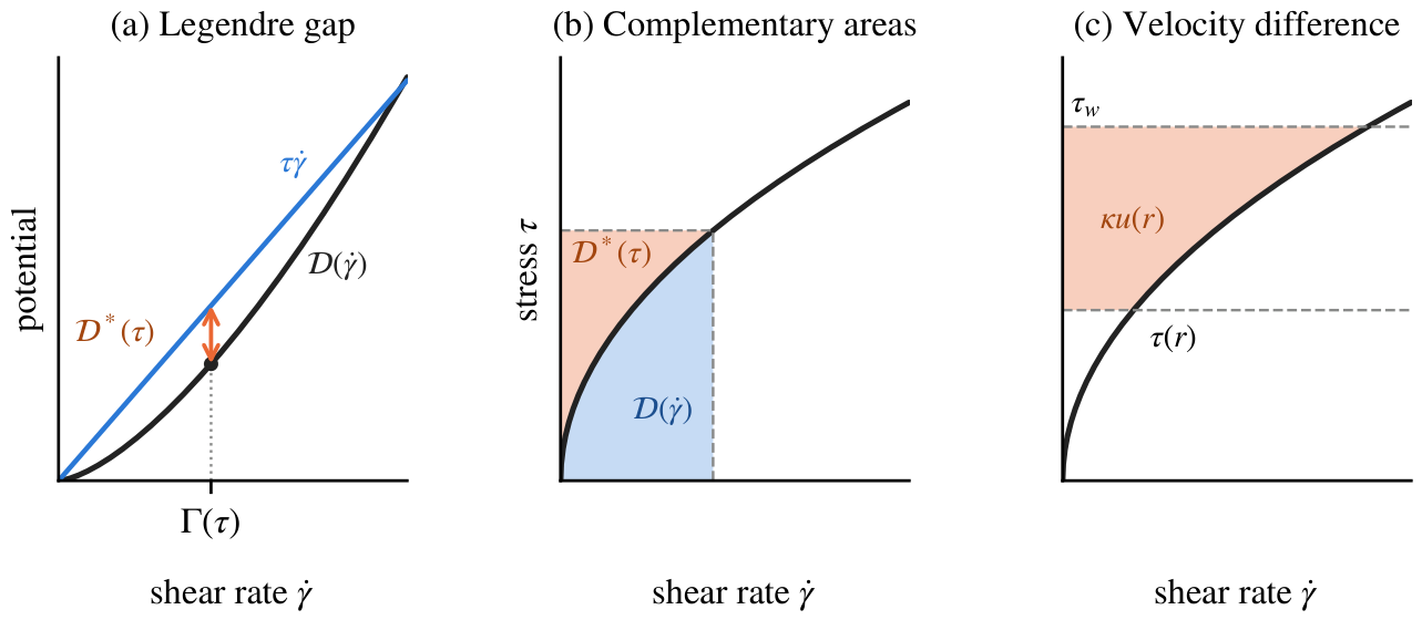
Figure 2.
Flat and cornered potentials in tube flow. (a) Complementary potentials for a Newtonian reference (), a Bingham fluid (, ) and a fluid with a stress plateau. The plateau is for , with slopes 2 and 1 below and above it. (b) Corresponding profiles at , each normalized by its own centreline velocity. The Bingham flat interval gives a plug of radius ; the plateau corner gives a velocity kink at . All quantities are nondimensional, with .
Figure 2.
Flat and cornered potentials in tube flow. (a) Complementary potentials for a Newtonian reference (), a Bingham fluid (, ) and a fluid with a stress plateau. The plateau is for , with slopes 2 and 1 below and above it. (b) Corresponding profiles at , each normalized by its own centreline velocity. The Bingham flat interval gives a plug of radius ; the plateau corner gives a velocity kink at . All quantities are nondimensional, with .
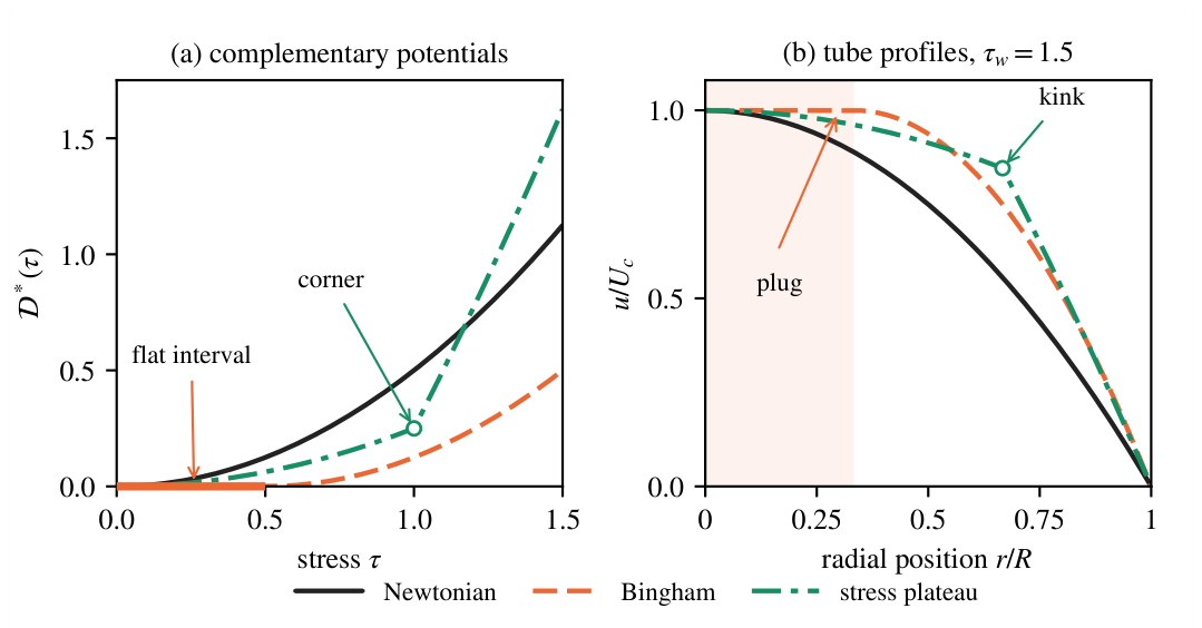
Figure 3.
Complementary potentials and their velocity profiles. (a,b) Potentials from the constitutive models (lines), compared with from independent integration of (circles). (c,d) Corresponding velocities from (8) and direct integration. Left: Carreau–Yasuda fluid with , , , , , ; panel (c) includes the bounds in Section 3.5. Right: Herschel–Bulkley fluid with , , , . Shading marks the flat potential and its corresponding plug. All quantities are nondimensional, with .
Figure 3.
Complementary potentials and their velocity profiles. (a,b) Potentials from the constitutive models (lines), compared with from independent integration of (circles). (c,d) Corresponding velocities from (8) and direct integration. Left: Carreau–Yasuda fluid with , , , , , ; panel (c) includes the bounds in Section 3.5. Right: Herschel–Bulkley fluid with , , , . Shading marks the flat potential and its corresponding plug. All quantities are nondimensional, with .
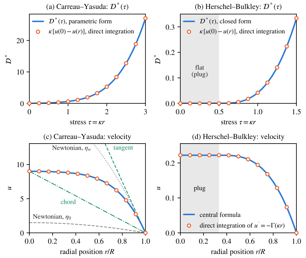
Figure 4.
From the local complementary potential to the pressure–flow response. (a) Cross-sectional potential for a Herschel–Bulkley fluid with , , and . (b) Flow rate . Shading marks , where both quantities vanish. The orange tangent in (a) has slope equal to the flow rate at the marked load in (b). The curves illustrate (22)–(23) using the constitutive potential; all quantities are nondimensional.
Figure 4.
From the local complementary potential to the pressure–flow response. (a) Cross-sectional potential for a Herschel–Bulkley fluid with , , and . (b) Flow rate . Shading marks , where both quantities vanish. The orange tangent in (a) has slope equal to the flow rate at the marked load in (b). The curves illustrate (22)–(23) using the constitutive potential; all quantities are nondimensional.
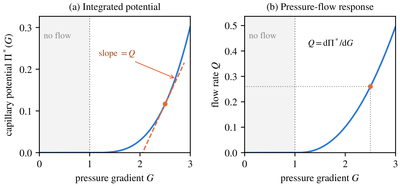
Figure 5.
Synthetic velocimetry for the Herschel–Bulkley case in Figure 3. (a) Velocity samples with independent Gaussian noise of standard deviation . (b) Potential values obtained from centreline-to-local velocity differences. (c) Inverse flow curve; circles are interior central differences of the noisy velocities. Dashed curves are the generating reference and blue curves are the regularized reconstruction from the same noisy profile. Shading gives the pointwise 5th–95th percentile range of reconstructions from 200 additional noise realizations with the same regularization weight. This range describes noise variability in the simulation, not an experimental confidence interval. The dotted line marks the true plug edge, which is not prescribed to the reconstruction. Axes are normalized by the reference values , and .
Figure 5.
Synthetic velocimetry for the Herschel–Bulkley case in Figure 3. (a) Velocity samples with independent Gaussian noise of standard deviation . (b) Potential values obtained from centreline-to-local velocity differences. (c) Inverse flow curve; circles are interior central differences of the noisy velocities. Dashed curves are the generating reference and blue curves are the regularized reconstruction from the same noisy profile. Shading gives the pointwise 5th–95th percentile range of reconstructions from 200 additional noise realizations with the same regularization weight. This range describes noise variability in the simulation, not an experimental confidence interval. The dotted line marks the true plug edge, which is not prescribed to the reconstruction. Axes are normalized by the reference values , and .
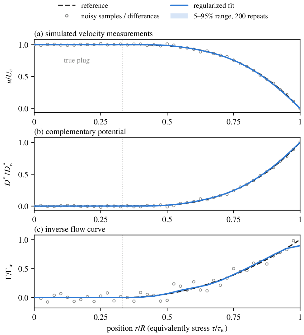
Figure 6.
Stress resolution of finite-interval shear-rate averages. Each reporting interval has width and is plotted at its midpoint. Curves give the 90th percentile of the absolute relative average-rate error over 200 realizations: (a) four fluids at 1% velocity noise; (b) Herschel–Bulkley at three noise levels. Filled symbols meet the illustrative 10% criterion; open symbols exceed it. The grey vertical band in (b) marks the true plug. Only whole intervals on the true yielded branch are assessed, using the true curve for assessment only. Here , , and the weight is reselected per profile. These conditional errors are not experimental confidence limits.
Figure 6.
Stress resolution of finite-interval shear-rate averages. Each reporting interval has width and is plotted at its midpoint. Curves give the 90th percentile of the absolute relative average-rate error over 200 realizations: (a) four fluids at 1% velocity noise; (b) Herschel–Bulkley at three noise levels. Filled symbols meet the illustrative 10% criterion; open symbols exceed it. The grey vertical band in (b) marks the true plug. Only whole intervals on the true yielded branch are assessed, using the true curve for assessment only. Here , , and the weight is reselected per profile. These conditional errors are not experimental confidence limits.
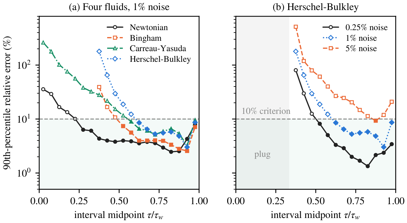
Figure 7.
Herschel–Bulkley wall-rate reliability at 1% velocity noise, and . Both panels show signed wall-rate bias. (a) Sensitivity to a multiplier of the Figure 5 reference weight, held fixed across realizations; retains shape constraints without a slope penalty. The horizontal axis is linear from 0 to 0.1 and logarithmic above 0.1. (b) Loss of near-wall observations, with weight reselection per profile and the exact no-slip wall velocity retained. The horizontal coordinate is . Lines are medians and shading gives 5th–95th percentile ranges over 200 realizations.
Figure 7.
Herschel–Bulkley wall-rate reliability at 1% velocity noise, and . Both panels show signed wall-rate bias. (a) Sensitivity to a multiplier of the Figure 5 reference weight, held fixed across realizations; retains shape constraints without a slope penalty. The horizontal axis is linear from 0 to 0.1 and logarithmic above 0.1. (b) Loss of near-wall observations, with weight reselection per profile and the exact no-slip wall velocity retained. The horizontal coordinate is . Lines are medians and shading gives 5th–95th percentile ranges over 200 realizations.
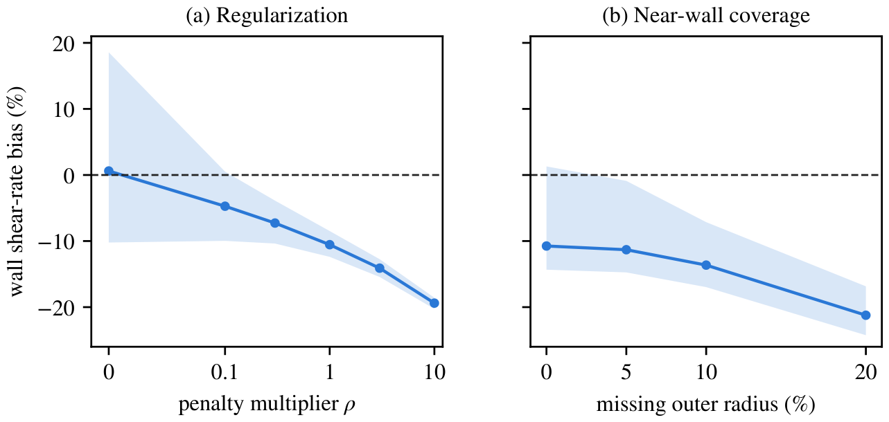
Figure 8.
Stress calibration and plug detectability. (a) Shear-rate bias at the fixed true stress . The dashed curve is the calibration-only prediction from (40); the blue curve and shading are the median and 5th–95th percentiles from 200 regularized noisy profiles, including baseline reconstruction bias. Here and , with weight reselection. (b) Two-point noise scale relative to the yielded-shell width, from (43) for , , , and , with varying yield stress. Curves use fixed relative noise or fixed absolute noise ; symbols mark the archived noise conditions. A ratio of unity means that the total shell velocity drop equals the threshold for two independent noisy measurements. This is a planning scale, not a confidence interval for a recovered plug edge.
Figure 8.
Stress calibration and plug detectability. (a) Shear-rate bias at the fixed true stress . The dashed curve is the calibration-only prediction from (40); the blue curve and shading are the median and 5th–95th percentiles from 200 regularized noisy profiles, including baseline reconstruction bias. Here and , with weight reselection. (b) Two-point noise scale relative to the yielded-shell width, from (43) for , , , and , with varying yield stress. Curves use fixed relative noise or fixed absolute noise ; symbols mark the archived noise conditions. A ratio of unity means that the total shell velocity drop equals the threshold for two independent noisy measurements. This is a planning scale, not a confidence interval for a recovered plug edge.
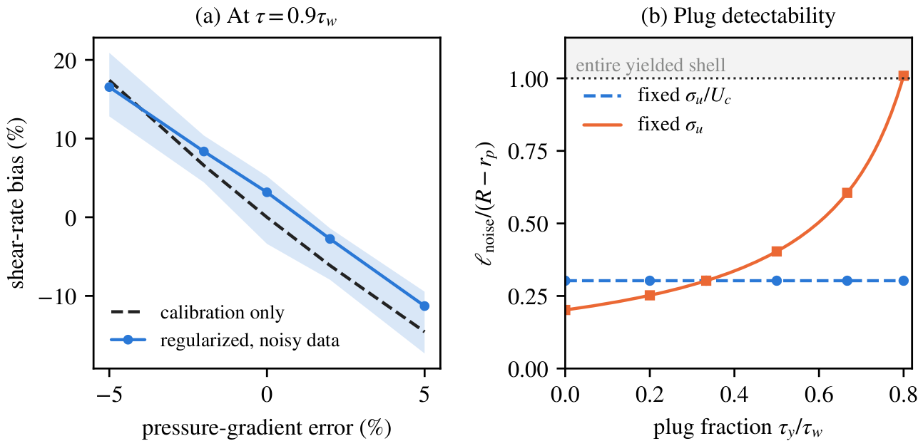
Figure 9.
Wall slip and geometric scope of the complementary potential. (a) Herschel–Bulkley tube profiles with and without a prescribed slip velocity , at , , , and . Velocities use the no-slip centreline value ; the grey band marks the bulk plug. (b) Centreline-to-local velocity differences give the same normalized potential for both profiles: the line and circles overlap. (c) Signed annular stresses for power-law fluids with , or , , and . Both walls satisfy no slip; circles mark the resulting zero-stress radii. The dotted line is the filled-tube reference . (d) An exact Newtonian example in the ellipse , with , , and . Arrows show transverse shear stress , not fluid velocity. Shading and labelled contours show ; the local potential must be integrated over the cross-section. All quantities are nondimensional.
Figure 9.
Wall slip and geometric scope of the complementary potential. (a) Herschel–Bulkley tube profiles with and without a prescribed slip velocity , at , , , and . Velocities use the no-slip centreline value ; the grey band marks the bulk plug. (b) Centreline-to-local velocity differences give the same normalized potential for both profiles: the line and circles overlap. (c) Signed annular stresses for power-law fluids with , or , , and . Both walls satisfy no slip; circles mark the resulting zero-stress radii. The dotted line is the filled-tube reference . (d) An exact Newtonian example in the ellipse , with , , and . Arrows show transverse shear stress , not fluid velocity. Shading and labelled contours show ; the local potential must be integrated over the cross-section. All quantities are nondimensional.
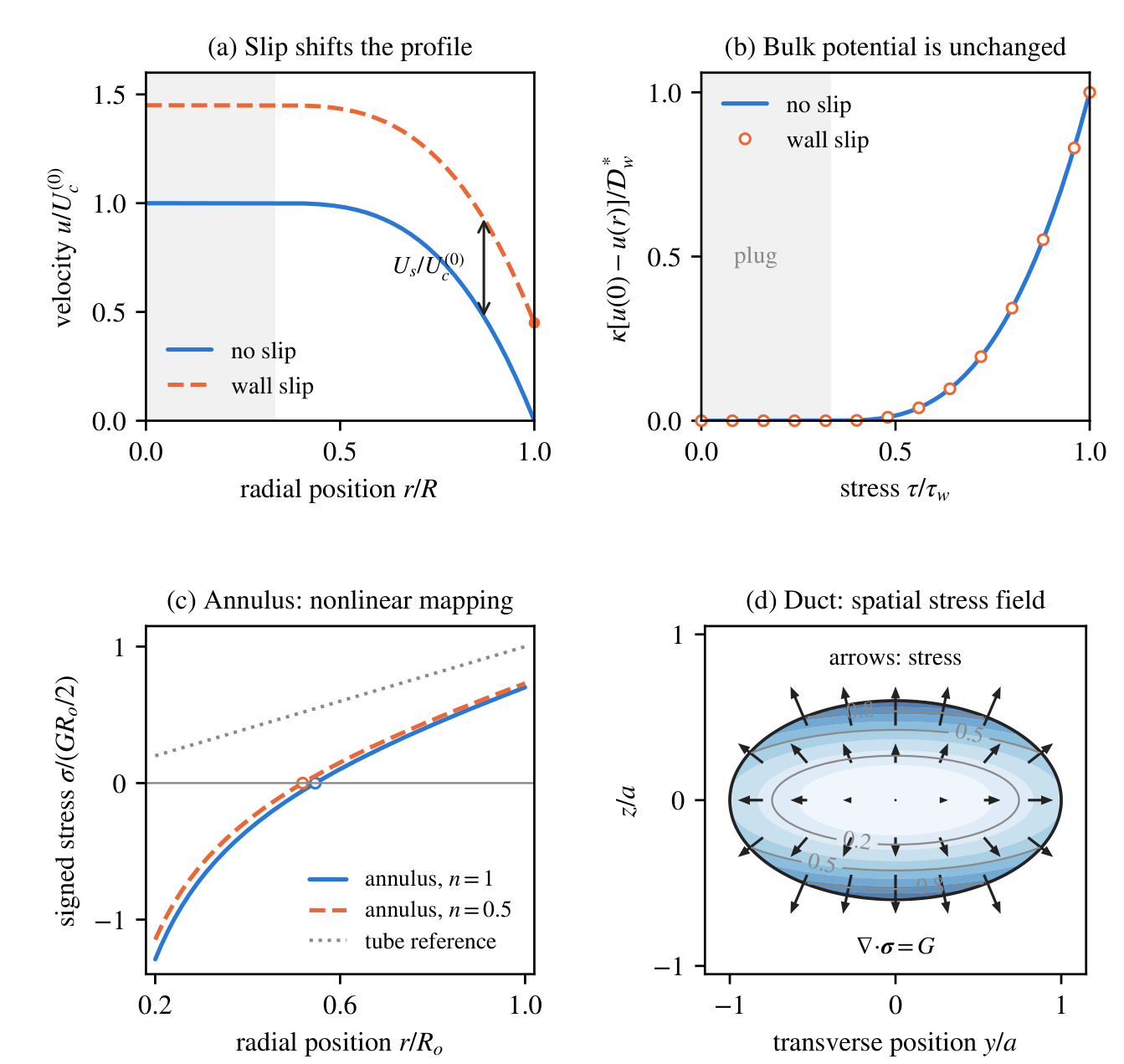

Table 1.
Complementary potentials used in the applications, with . Here . The Herschel–Bulkley entry assumes and includes Bingham flow when . For the two saturating laws, and ; the potential is outside its stated stress domain.
Table 1.
Complementary potentials used in the applications, with . Here . The Herschel–Bulkley entry assumes and includes Bingham flow when . For the two saturating laws, and ; the potential is outside its stated stress domain.
| Model | Flow curve | |
|---|---|---|
| Newtonian reference | ||
| Herschel–Bulkley | ||
| Carreau–Yasuda | , (17) | Parametric evaluation from (10) |
| Saturating Carreau | , | |
| Saturating Cross | , |
Table 2.
Median reconstruction errors over 200 independent noise realizations for each fluid. Here , and . The regularization weight is reselected for each realization. , , and are defined in Section 5.3. The wall-rate column is a signed bias.
Table 2.
Median reconstruction errors over 200 independent noise realizations for each fluid. Here , and . The regularization weight is reselected for each realization. , , and are defined in Section 5.3. The wall-rate column is a signed bias.
| Fluid | (%) | (%) | (%) | (%) |
|---|---|---|---|---|
| Newtonian | 0.44 | 1.79 | 0.57 | -7.31 |
| Bingham | 0.54 | 2.06 | 0.40 | -7.51 |
| Carreau–Yasuda | 0.60 | 2.08 | 0.37 | -12.21 |
| Herschel–Bulkley | 0.52 | 2.25 | 0.35 | -10.75 |
Table 3.
Stress resolution in the synthetic tests at and . Noise is . Each reporting interval has width . Listed ranges are unions of whole intervals whose 90th-percentile relative average-rate error is at most 10%. The final two columns give 90th-percentile errors for the last interval average and the point wall rate. These are estimator-dependent simulation results using the true curve for assessment, not confidence limits for measured data.
Table 3.
Stress resolution in the synthetic tests at and . Noise is . Each reporting interval has width . Listed ranges are unions of whole intervals whose 90th-percentile relative average-rate error is at most 10%. The final two columns give 90th-percentile errors for the last interval average and the point wall rate. These are estimator-dependent simulation results using the true curve for assessment, not confidence limits for measured data.
| Fluid | Noise (%) |
Passing |
Last average (%) |
Wall rate (%) |
|---|---|---|---|---|
| Newtonian | 1 | 0.25–1.00 | 7.9 | 10.1 |
| Bingham | 1 | 0.50–1.00 | 7.1 | 10.1 |
| Carreau–Yasuda | 1 | 0.55–1.00 | 9.6 | 15.3 |
| Herschel–Bulkley | 0.25 | 0.50–1.00 | 3.4 | 7.6 |
| Herschel–Bulkley | 1 | 0.60–1.00 | 8.6 | 13.9 |
| Herschel–Bulkley | 5 | 0.85–0.90 | 20.9 | 26.9 |
Table 4.
Wall-rate assessment on the same baseline 200 profiles per fluid. The declared upper log-slope bound applies over and is rounded upward from the generating law, supplying additional constitutive information. Width selection uses candidates and simultaneous 95% brackets. Errors are 90th percentiles of absolute relative error; coverage is empirical, and width is the median bracket width divided by the true wall rate. The regularized estimates do not use the declared slope bound.
Table 4.
Wall-rate assessment on the same baseline 200 profiles per fluid. The declared upper log-slope bound applies over and is rounded upward from the generating law, supplying additional constitutive information. Width selection uses candidates and simultaneous 95% brackets. Errors are 90th percentiles of absolute relative error; coverage is empirical, and width is the median bracket width divided by the true wall rate. The regularized estimates do not use the declared slope bound.
| Fluid | Midpoint error (%) |
Regularized error (%) |
Coverage (%) |
Width (%) |
|
|---|---|---|---|---|---|
| Newtonian | 1 | 6.7 | 10.1 | 100.0 | 24.6 |
| Bingham | 1.75 | 5.1 | 10.1 | 100.0 | 26.3 |
| Carreau–Yasuda | 3.5 | 6.9 | 15.3 | 100.0 | 31.2 |
| Herschel–Bulkley | 3.5 | 6.0 | 13.9 | 100.0 | 30.1 |
Disclaimer/Publisher’s Note: The statements, opinions and data contained in all publications are solely those of the individual author(s) and contributor(s) and not of MDPI and/or the editor(s). MDPI and/or the editor(s) disclaim responsibility for any injury to people or property resulting from any ideas, methods, instructions or products referred to in the content. |
© 2026 by the author. Licensee MDPI, Basel, Switzerland. This article is an open access article distributed under the terms and conditions of the Creative Commons Attribution (CC BY) license.
Copyright: This open access article is published under a Creative Commons CC BY 4.0 license, which permit the free download, distribution, and reuse, provided that the author and preprint are cited in any reuse.