

Submitted:
16 October 2026
Posted:
20 October 2026
You are already at the latest version
Abstract
Industrial machines, such as centrifugal pumps, accumulate large volumes of signals under healthy operating conditions long before representative fault data become available. However, the value of these normal-operation signals for subsequent fault diagnosis remains insufficiently explored. This work introduces a One-Class Signal World Model (OC-SWM), whose encoder is learned exclusively from healthy-operation data and subsequently transferred to diagnostic tasks when only a limited number of fault examples are available. The method constructs a sequence of latent states from each healthy vibration signal with a teacher–student–predictor architecture to learn their dynamics through latent-state prediction. The resulting encoder is then coupled with an attention-based readout and adapted using a small set of fault signals. Experiments on a ten-stage vertical centrifugal pump under six hydraulic regimes show that one-class pretraining yields a macro-F1 of 0.814 with only 30 labeled examples per health condition and a normalized area under the label-efficiency curve of 0.947, with the proposed method outperforming contrastive and adversarial alternatives and matching a regime-conditioned variant with lower dispersion across folds. Furthermore, the pretrained representation captures the structure of the hydraulic regimes before any fault-supervised adaptation, even though regime information is not explicitly provided during pretraining. This finding indicates that OC-SWM captures physically meaningful information about the machine operating state while providing a reusable representation for label-efficient fault diagnosis.
Keywords:
centrifugal pump
; fault diagnosis
; self-supervised learning
; predictive representation learning
; healthy-only pretraining
; limited labeled data
; vibration measurement
; condition monitoring
1. Introduction
Centrifugal pumps are essential equipment in water distribution, energy conversion, chemical processing, and manufacturing. Their availability directly affects production continuity, energy consumption, and maintenance costs. However, vibration-based diagnosis is challenging because the measured response depends on several physical mechanisms, including rotor dynamics, hydraulic loads, and operating conditions [1]. This complexity increases in multistage configurations, where excitation sources are distributed along the shaft and their transmission changes through the pump structure [2]. Consequently, the same mechanical condition can produce different vibration responses under different hydraulic regimes.
Deep learning has reduced the dependence of pump diagnosis on manually selected indicators. One-dimensional convolutional networks can learn directly from raw signals [3], while other approaches transform vibration into time–frequency representations that are subsequently processed by two-dimensional convolutional networks [4]. For example, spectrograms have been used for monoblock pump diagnosis [5]. Pretrained image models have also been transferred to pump scalogram analysis [6]. Defect-sensitive waveform fragments have been integrated into end-to-end classifiers [7]. In addition, multi-channel fusion has improved vertical-pump diagnosis [8], while studies on compound faults and imbalanced class distributions have extended these methods to more demanding scenarios [9,10]. Together, these works show that learned representations can extract relevant diagnostic information. However, most assume a setting in which representative labeled examples of machinery faults are already available.
This assumption does not reflect the temporal sequence in which data typically become available in industrial applications. Large volumes of healthy signals can accumulate during commissioning and routine operation. In contrast, faults appear later and much less frequently. Some faults are also costly to reproduce, unsafe, or destructive. As a result, labeled fault datasets are usually much smaller than the amount of normal-operation data available. Limited-label diagnosis has been addressed through hierarchy-guided transfer [11], attention-based meta-transfer [12], and prior-knowledge-guided adaptation [13]. These strategies reduce the demand for labeled data, but they typically focus on an already defined task or on datasets with available fault-related information. An earlier stage can also be exploited: the period in which only signals accumulated during healthy operation are available. This possibility is particularly relevant to edge-based monitoring systems [14] and transfer-enabled digital twins [15], where a representation learned during routine operation can be retained and reused when new diagnostic needs arise.
Self-supervised learning (SSL) provides a mechanism for exploiting available signals before labeled examples become available. Machinery SSL has been studied through transformation prediction, contrastive learning, temporal consistency, and time–frequency objectives [16,17]. Similarly, general time-series methods can learn multiscale temporal structure without labels from the downstream task [18]. In multistage centrifugal pumps, contrastive pretraining has also demonstrated improved generalization across operating conditions [19]. However, in the fault-diagnosis studies by Chen et al. [17] and Wu et al. [19], the unlabeled pretraining dataset includes fault-condition signals, allowing the model to acquire fault-related information before supervised training. The healthy-only setting poses a different problem because pretraining lacks future fault conditions. The central question is therefore whether structure learned exclusively from healthy operation can be reused when fault conditions later emerge. Recent work has begun to investigate this setting in bearings, where substantial prior knowledge about discriminative characteristics is available [20]. Its usefulness when learning directly from raw signals in more complex machinery, such as multistage centrifugal pumps operating under different hydraulic regimes, remains insufficiently characterized.
Latent predictive learning provides another approach that can exploit signals before fault labels become available. However, its main developments originate from domains far removed from machinery monitoring. BYOL introduced a slowly updated target network to stabilize self-supervised learning in images [21]. Data2vec subsequently extended contextualized representation prediction to modalities including speech, text, and images [22]. I-JEPA further developed this principle by predicting masked regions directly in visual representation space [23]. These formulations were originally developed outside the machinery vibration domain. Vibration measurements are high-frequency one-dimensional signals with transient, periodic, and cyclostationary content, and their structure is governed by mechanical dynamics and operating conditions. A previous Signal-World-Model adapted this principle to cyclostationary vibration under limited label availability [24]. That study addressed a different data chronology from the one considered here. The present work focuses on the earlier stage, when learning occurs before fault signals become available. We address this setting through a One-Class Signal World Model (OC-SWM) pretrained exclusively on healthy vibration. We then transfer the resulting encoder to a multiclass diagnostic task with a limited number of fault examples.
Operating conditions constitute another central aspect of this problem. The hydraulic regime affects both healthy vibration and the resulting fault signature. Therefore, representation learning must account for this information. Domain-adversarial training seeks to reduce domain information in the learned representation [25,26]. In contrast, condition-aware models explicitly incorporate operating-regime information [27]. In this work, we evaluate both strategies alongside the standard OC-SWM. The proposed model uses signals acquired across hydraulic regimes and learns directly from vibration, excluding regime identity from the model input.
From this perspective, OC-SWM represents the machine as a partially observable dynamical system. Its latent state integrates mechanical interactions among components, the system’s temporal evolution, and the conditions that modulate its response. These conditions include both the operating regime and the health state. Vibration signals provide an observable manifestation of this state and its evolution. Consequently, signals acquired under different operating regimes and health conditions correspond to different trajectories of the same physical system. Pretraining on healthy vibration provides observations from one region of this dynamical space before fault examples become available. From these observations, OC-SWM learns contextual relationships among latent states that characterize the mechanisms governing the vibration response. This representation embeds hydraulic regime and health condition as factors that modulate the observed trajectories. When fault conditions subsequently emerge, the learned encoder provides an initial representation of the same machine and its underlying dynamics that can be adapted using a limited number of labeled fault signals. The main contributions of this work are:
- We propose a One-Class Signal World Model (OC-SWM) trained exclusively on healthy vibration. The model represents each signal as a sequence of latent states and learns their contextual relationships during normal operation.
- We introduce a lightweight attention-based diagnoser that reuses the representation learned by OC-SWM. A learnable classification vector integrates the complete sequence of transferred states. We also evaluate whether an auxiliary objective that incorporates mechanical knowledge through health-condition families improves the primary multiclass diagnostic task.
- We establish an experimental protocol that separates examples at the level of complete acquisitions. Independent acquisitions define the training, validation, and test sets, and the folds preserve the same separation unit. This strategy maintains independence among the data partitions and controls information leakage between windows originating from the same acquisition. We apply the same protocol consistently to all comparison models, variants, and ablation studies.
- We conduct a visibility study of the hydraulic-state structure learned by OC-SWM during pretraining on healthy vibration. The analysis evaluates how the representation encodes the organization of different hydraulic regimes before fault-supervised adaptation. This study characterizes the physical information that emerges in the latent space and its relationship to the encoder’s transferability.
2. Methodology
OC-SWM separates representation learning from its subsequent adaptation to a diagnostic task. During pretraining, an encoder transforms vibration into a sequence of latent states and learns relationships among different regions of this sequence through a teacher–student–predictor architecture. Representation learning uses healthy signals exclusively. After pretraining, the student encoder is retained and coupled with a lightweight attention mechanism to use the learned representation with a limited set of labeled signals.
2.1. One-Class Formulation
Let denote a vibration signal with L samples and C channels. The dataset available for representation learning is defined as
and contains exclusively signals acquired during healthy pump operation. These signals may correspond to different operating conditions. Therefore, contains different responses of the same machine within the healthy region of its operating space. Because the proposed model uses vibration as its only input, it must learn the structure associated with operating conditions directly from the signal.
The transferable encoder comprises a convolutional state encoder and a contextual encoder , with parameters . The first component employs the Non-Overlapping Receptive Field (NORF) strategy to prevent information leakage when constructing states from vibration signals [24]. Given an input x, it generates an ordered sequence
where each represents a temporal region of the signal. A fixed positional encoding P preserves the order of these observations, and the contextual encoder produces
While contains local vibration information, incorporates the relationships between that observation and the remaining available trajectory.
2.2. State Construction Using NORF
Vibration contains information distributed across different temporal scales. Local events may appear at different positions within a window, whereas longer-duration patterns arise from interactions among multiple mechanical responses. For this reason, first employs a convolutional hierarchy with overlapping receptive fields. This structure captures local characteristics without requiring a fixed position within the signal. NORF then organizes the extracted features into final states with separated temporal support.
Let D denote the number of layers used for hierarchical extraction. For layer i, , , and denote the kernel size, stride, and dilation, respectively. The cumulative displacement and receptive field , both expressed with respect to the original signal, evolve as
After these layers, NORF incorporates a state-forming stage with a unit kernel. Its stride is defined as
such that . Consequently, consecutive final states correspond to distinct temporal supports in the original signal. The preceding layers retain the overlap needed to extract local patterns, whereas NORF separates the observations. When a state is selected as a predictive target, its temporal support remains separated from that of the adjacent states that remain visible. Prediction must therefore rely on relationships among different vibration regions, reducing the possibility of recovering the target from shared local content. The output of this stage corresponds to the sequence U in Equation (2), which is subsequently contextualized by according to Equation (3).
2.3. Predictive Learning in Latent Space
Pretraining uses a teacher–student–predictor architecture. The student contains the encoder whose parameters are subsequently transferred. The teacher, denoted by , has the same structure and provides the target representations. A predictor receives the states available to the student and estimates the representations associated with the hidden regions. The entire process uses signals from , and the learning objective is defined directly in latent space.
For each input, independent predictive tasks are generated. Let denote the set of positions in the latent trajectory. Task m selects a contiguous block of positions,
where contains the target positions and the visible positions. We select the initial position independently. Therefore, different predictive tasks associated with the same signal can explore different regions of the trajectory, and their target blocks may overlap.
From this point onward, for any sequence A indexed by , the notation denotes the subsequence formed by the positions in while preserving their temporal order. The teacher processes the complete sequence and generates
The sequence contains the contextualized teacher states associated with the target positions of task m. In contrast, the student retains the local observations corresponding to and contextualizes them as
Thus, contains the context available for prediction, whereas contains the representations to be inferred. The teacher establishes its targets from the complete trajectory, while each student task solves a different contextual prediction problem for the same signal.
The predictor operates in an internal space of dimension . The states in are normalized and projected through . Positions corresponding to are represented by a learnable vector q. Both the visible states and the target-position markers preserve their original locations through a positional encoding . The predictor input is constructed as
where denotes Layer Normalization applied independently to each state along the latent dimension d, is the positional encoding used in the predictor space, and denotes concatenation. The visible elements occupy the first part of , whereas the last elements correspond to the positions in . The positional encoding preserves the correspondence between each predictor element and its position in the original trajectory.
The Transformer contextualizes . By construction, the last outputs correspond to the target positions and are projected back into the encoder space,
The OC-SWM objective directly compares the predicted and target states,
where stops gradient propagation through the teacher targets.
The student and predictor parameters are updated by minimizing . After each update, the teacher parameters evolve through an exponential moving average,
where controls how rapidly the teacher follows the student.
After pretraining, denotes the parameters learned by the convolutional state encoder and the student contextual encoder. This encoder constitutes the transferable component of OC-SWM. The teacher and predictor are used exclusively for self-supervised learning. Figure 1 illustrates the pretraining workflow, from sliding-window segmentation of healthy signals to teacher–student latent-state prediction.
2.4. Attention-Based Transfer to Diagnosis
When a labeled dataset subsequently becomes available, with , the encoder is initialized with the parameters . For each signal, it produces the contextualized trajectory . The supervised stage uses the complete sequence and learns to integrate its states to distinguish the K diagnostic conditions.
Aggregation is performed using a learnable classification vector and a lightweight attention encoder . The vector is prepended to the transferred trajectory, and its contextualized representation is used as a summary of the sequence,
where selects the output associated with the classification vector. The aggregation can therefore depend on relationships among the transferred states and on their relevance to the diagnostic task.
A classification head produces the logits . Adaptation is optimized using
and the estimated condition is obtained as .
Adaptation begins by optimizing the new diagnostic modules while preserving the transferred representation. Later, the encoder is included in joint optimization to adapt its states to the conditions represented in the labeled dataset. This procedure first lets the attention mechanism and classifier learn to use the trajectory obtained during pretraining and then refines the full representation for the diagnostic task.
3. Experimental Study on a Multistage Centrifugal Pump
The experimental study evaluates three aspects of the proposed approach. First, it determines whether a representation learned exclusively from healthy vibration can be transferred to a multiclass diagnostic task under different labeled-signal budgets. Second, it analyzes the effect of different strategies for handling the operating condition during representation learning. Finally, it examines whether the encoder can access physical information associated with the hydraulic state before supervised adaptation.
3.1. Experimental Platform and Acquisition Conditions
The experiments were conducted on a ten-stage Gulf 3SV10GE4F20 vertical multistage centrifugal pump driven by a 1.5 kW three-phase motor. The pump has a nominal flow rate of 15 gallons per minute (GPM) and a nominal motor speed of 3500 rpm. Figure 2 shows the experimental pump, the sensor locations, and the data-acquisition hardware.
Acceleration signals were acquired using the A1 IMI Sensors 603C01 accelerometer with a range. An NI CompactDAQ-9188 chassis housed the acquisition modules. The A1 channel was sampled through an NI 9234 module at 50 kS/s, and each vibration acquisition lasted 10 s, producing 500,000 samples. The P2 discharge-pressure channel was sampled through an NI 9205 module at 25 kS/s to characterize the hydraulic operating conditions. OC-SWM and its diagnostic readout used A1 vibration as their signal input.
The motor operated at a constant electrical frequency of 60 Hz. The hydraulic load was varied through the discharge valve to establish six regimes, S1–S6. The valve positions were defined under healthy baseline operation at reference discharge pressures of approximately 5.5, 6.5, 7.5, 8.5, 9.5, and 10.4 bar, with a tolerance of bar.
The experiments consider seven diagnostic classes: Healthy operation, Inlet pitting I, Inlet pitting II, Outlet pitting I, Outlet pitting II, Severe blockage, and Severe imbalance. The four pitting classes differ in damage location, number of affected stages, and the severity associated with each stage. Severe blockage and Severe imbalance correspond to faults distributed across six consecutive stages. Ten complete and independent acquisitions, denoted R1 through R10, are available for every combination of diagnostic class and hydraulic regime. Table 1 presents the physical configurations corresponding to the classes used.
3.2. Dataset Construction
We use the complete acquisition as the separation unit for training, validation, and test sets. Windows extracted from the same acquisition always remain within the same subset. This criterion prevents related segments of the same signal from appearing simultaneously during model fitting and evaluation. We apply the same procedure to all models, comparison methods, variants, and controls considered in this study. The ten repetitions are organized through eight circular rotations. In each fold, five acquisitions are used for training, two for validation, and three for testing. Table 2 shows the assignments. The acquisitions are segmented into windows of 8192 samples, equivalent to 163.84 ms, corresponding to approximately 9.6 pump cycles of 17.14 ms each. This constitutes the common preprocessing procedure for all models.
We extract windows with a displacement of 50 samples. Each 500,000-sample acquisition produces 9837 windows, so each fold contains 295,110 healthy windows for representation learning. Validation and test acquisitions are segmented using a displacement of 8192 samples, producing 61 non-overlapping windows per complete signal. Consequently, each fold contains 5124 validation windows and 7686 test windows. The test set includes 1098 windows per diagnostic class and 1281 windows per hydraulic regime. We evaluate diagnostic transfer with 30, 75, 150, and 300 labeled windows per class. The deterministic construction of these budgets remains unchanged across all methods within a fold. Therefore, each comparison uses exactly the same labeled training signals and the same validation and test sets.
3.3. OC-SWM Implementation
The convolutional state encoder consists of six layers, whose configurations are shown in Table 3. The first five form the convolutional hierarchy with overlapping receptive fields. The sixth implements NORF and produces the final state sequence. All convolutions include bias, use unit dilation, and are followed by Layer Normalization and ReLU.
The cumulative output stride is 192 samples, and the receptive field of each state is 187 samples. Therefore, the 43 final states represent distinct temporal supports. The contextual encoder operates at dimension and uses one Transformer layer, one attention head, a 2048-unit feed-forward layer, ReLU activation, post-normalization, and fixed sinusoidal positional encoding. The predictor projects the states from 128 dimensions to an internal dimension of . It uses one Transformer layer with one attention head, 2048 units in the feed-forward layer, ReLU, post-normalization, and 0.1 dropout. Its output is projected back to 128 dimensions. For each signal, independent predictive tasks are generated. Each task selects a block of consecutive states and retains the remaining 22 states as context.
The diagnoser uses the 43 transferred states and a learnable classification vector. The readout contains one Transformer layer with dimension 128, eight attention heads, a 256-unit feed-forward layer, ReLU activation, post-normalization, and 0.3 dropout. The classification-vector representation directly feeds the seven-class head.
3.4. Training and Transfer
We perform OC-SWM pretraining for 20 epochs using AdamW with a batch size of 512. The learning rate follows cosine decay from to , while weight decay increases linearly from 0.04 to 0.40. The teacher parameters are updated after each mini-batch through EMA, with an initial momentum of 0.9996 that gradually increases during training. AdamW uses and . The encoder obtained after 20 epochs is denoted by and serves as the state for subsequent transfers.
Diagnostic adaptation is performed for 150 epochs using AdamW with a batch size of 105. The transferred encoder uses a learning rate of , while the new diagnostic modules use ; both remain constant. The weight decay is 2.5. During the initial adaptation period, the contextual encoder remains frozen while the new diagnostic modules are optimized on the transferred representation. Encoder updates begin after the warm-up period, after which the system is optimized jointly. Test evaluation uses the model that achieves the highest macro-F1 on the validation acquisitions.
3.5. Comparison Methods and OC-SWM Variants
The first reference is a supervised ResNet1D [28]. This model characterizes the performance obtained when learning depends exclusively on the labeled signals available under each budget. As a self-supervised reference, we use the normalized temperature-scaled cross-entropy (NT-Xent) objective, which has been applied to vibration-based bearing diagnosis [29]. Our NT-Xent baseline is trained exclusively on the same Healthy operation acquisitions used by OC-SWM. Thus, both approaches follow the same data chronology and use the same healthy-only dataset. For NT-Xent, each healthy signal generates two independent views through circular translation, Gaussian noise, sign inversion, amplitude scaling, and DC offset. After the convolutional encoder, contextual encoder, and mean pooling, a two-layer projection head produces normalized representations. For a batch containing N source signals, the objective is
where identifies the other view of the same signal and . Pretraining uses the same 20 epochs, batch size of 512, healthy acquisitions, regimes, and base architecture as OC-SWM. The transformation probabilities are 0.4 for translation, 0.9 for Gaussian noise at 8 dB SNR, 0.8 for sign inversion, 0.8 for amplitude scaling, and 0.5 for DC offset. We remove the projection head before diagnostic adaptation.
Two variants explicitly examine how the hydraulic regime is treated. RegimeCond-SWM incorporates regime information into the predictor during pretraining. Each regime is represented by a learnable 16-dimensional embedding that is added to the projected context with a scale factor of 0.3. The student encoder and teacher continue to process vibration alone. After pretraining, the conditioned predictor is removed and the diagnoser receives only signal-derived states. DANN-SWM adopts an adversarial strategy to reduce regime-related information in the representation [25]. A discriminator receives the contextualized states and predicts one of the six hydraulic regimes. The gradient-reversal coefficient increases linearly to 0.1 during the first 20% of pretraining. The objective combines the predictive loss, domain classification, and a term that penalizes differences in predictive loss across regimes,
This variant also uses a higher-capacity diagnoser with explicit regime information and CORAL alignment of its representations. The comparison evaluates whether a strategy that reduces hydraulic information during learning and explicitly incorporates it during diagnosis outperforms learning directly from vibration.
3.6. Transfer and Complexity Controls
Additional controls identify the contribution of the learned representation and the modules used during adaptation. SWM-Conv reuses the same healthy-only encoder and couples it to a simpler convolutional diagnoser. This comparison evaluates the contribution of the attention-based readout used in our proposed approach (SWM-Attn). The SWM-Conv diagnoser processes the sequence of 43 contextualized states, each of dimension 128, using two one-dimensional convolutions along the temporal axis. These layers have 32 and 16 output channels, respectively, and both use a kernel size of 7, a stride of 2, and ReLU activation, without padding. The sequence length decreases from 43 to 19 and then to 7. Global max pooling over the remaining temporal positions produces a 16-dimensional feature vector, which feeds a linear classifier with seven outputs corresponding to the health conditions.
We evaluate the contribution of the weights acquired during pretraining using a matched control. We train two models with the same diagnostic architecture and the same adaptation configuration. The first uses the encoder obtained after healthy-only pretraining, whereas the second restores the encoder initialization stored immediately before pretraining. Both models share the initialization of the new diagnostic modules, training data, example order, loss function, optimizer, learning rates, and number of epochs. In both cases, the encoder is trainable from the beginning. These matched models both use the auxiliary family supervision described below. Therefore, the initial encoder weights constitute the only difference between the two models.
For a metric m in fold f, the gain associated with healthy-only pretraining is defined as
where corresponds to the model initialized with the pretrained weights and to the model using the initialization prior to pretraining. The comparison also extends to individual decisions for each test window. For each example, we record whether both models classify it correctly or incorrectly. This produces four possible cases: correct only with pretrained weights, correct under both initializations, correct only with the initial weights, and incorrect under both. The analysis is performed globally and by diagnostic class and hydraulic regime.
The proposed SWM-Attn uses the health-condition classification loss without auxiliary family supervision. We evaluate explicit incorporation of mechanical-family knowledge as an additional control. Following the class order in Table 1, the mapping groups Inlet pitting I and Inlet pitting II into one family, Outlet pitting I and Outlet pitting II into another, and retains separate groups for Healthy operation, Severe blockage, and Severe imbalance. The control adds an auxiliary head to the classification-vector representation and uses the combined loss
with , activated after the first 50 adaptation epochs. The proposed SWM-Attn uses . This comparison determines whether explicitly providing the mechanical taxonomy contributes additional information beyond the representation obtained from the signals.
3.7. Metrics and Fold Aggregation
The primary metric is macro-F1, calculated as the mean F1 score across the seven classes. Label efficiency is summarized through the normalized area under the macro-F1 versus labeled-signal-budget curve,
where and denotes the test macro-F1 for each budget. In addition to overall performance, we analyze results by diagnostic class and hydraulic regime. Each configuration is trained independently across the eight folds, after which its mean value is calculated. We apply the same aggregation procedure to all results.
3.8. Hydraulic-State Visibility Study
The hydraulic-state visibility study examines whether the structure associated with the operating regime is accessible in latent space before fault-supervised adaptation. The encoder parameters remain frozen throughout this analysis. For each window, the contextualized states are averaged over time to obtain a vector . A linear probe based on ridge regression is then fitted. The fit uses only windows from the two validation acquisitions of each fold. The representations are standardized to zero mean and unit variance, while the documented hydraulic setpoint is standardized independently using the same validation data.
The fitting problem is expressed as
where contains the windows used to fit the probe, denotes the corresponding standardized representation, and is the standardized hydraulic setpoint associated with its regime. The regularization coefficient is selected by cross-validation over 25 logarithmically spaced values between and . The coefficient of determination quantifies the accessibility of the pressure scale associated with the regimes, while Spearman evaluates preservation of the S1–S6 ordering. We apply the same procedure to the different representations considered in the analysis.
4. Results and Discussion
4.1. Label-Efficient Multiclass Diagnosis
Figure 3 shows the test macro-F1 of the six evaluated systems under the four labeled-data budgets. SWM-Attn reaches , , , and with 30, 75, 150, and 300 windows per class, respectively. Its AULC is , followed by for RegimeCond-SWM, for SWM-Conv, for ResNet1D, for healthy-only NT-Xent, and for DANN-SWM. RegimeCond-SWM reaches mean values close to SWM-Attn but exhibits considerably greater dispersion across folds at the lower budgets. Therefore, SWM-Attn combines the highest AULC with stronger robustness among the two best-performing systems.
The differences are larger when supervision is more limited. With 30 windows, SWM-Attn reaches a macro-F1 of . With 75 windows, it increases to . Relative to ResNet1D, the absolute macro-F1 differences are , , , and for the four budgets. The progressive reduction in this difference indicates that pretraining is more valuable when the supervised task has fewer examples.
The macro-F1 values of Healthy-only NT-Xent are , , , and . Consequently, the differences relative to SWM-Attn are , , , and , while the AULC difference is 0.266. Both methods learn exclusively from healthy signals but use different objectives. NT-Xent organizes the space through consistency between transformed views. In contrast, OC-SWM learns by predicting contextualized regions along the latent trajectory, which may be more appropriate for inputs where the order of events matters. Under the same healthy-only setting, our approach generates a representation with greater transfer capability for the diagnostic task.
Table 4 summarizes the performance of SWM-Attn under each regime. With 30 labeled training examples per class, macro-F1 ranges from in S6 to in S2. S1–S3 achieve values between 0.854 and 0.876, whereas S4–S6 show progressively lower values. With 75 examples per class, all regimes reach at least 0.865. With 150 examples per class, the values range from 0.936 to 0.992, and with 300 from 0.967 to 0.997. The differences observed among regimes in the low-label setting decrease rapidly as supervision increases. S6 is the most challenging regime with 30 examples per class but reaches under the largest budget. Therefore, both the same representation and the same diagnoser can be adapted across all six regimes without explicitly introducing their identity into SWM-Attn.
The confusion matrices in Figure 4 show which fault types concentrate the diagnostic difficulty. With 30 windows, the correct-classification rates are 0.78 for Healthy operation, 0.72 for Inlet pitting I, 0.72 for Inlet pitting II, 0.90 for Outlet pitting I, 0.86 for Outlet pitting II, 0.95 for Severe blockage, and 0.77 for Severe imbalance. The largest individual confusion occurs when Inlet pitting II is classified as Outlet pitting II, with a mean rate of 0.12. Confusions also appear among the different pitting classes and, to a lesser extent, among Healthy operation, Severe imbalance, and Severe blockage.
With 300 windows, the diagonal increases to 0.98, 0.99, 0.98, 0.99, 0.99, 1.00, and 0.97 for the seven health conditions, respectively. The four pitting conditions are then clearly separated despite sharing related damage mechanisms and differing in location, number of affected stages, and severity. The same behavior is observed for Severe blockage and Severe imbalance, whose configurations involve multiple stages.
4.2. Effect of Healthy-Only Pretraining
Figure 5 isolates the contribution of the weights acquired during pretraining. We compare two models with the same diagnostic architecture and adaptation procedure. One starts from the healthy-pretrained encoder, while the other starts from the initialization stored before pretraining. The two models share the diagnostic-module initialization, labeled signals, training order, loss function, optimizer, learning rates, and number of epochs. In addition, we evaluate both on the same test windows. The difference in their performance measures the effect of the encoder initialization acquired during the 20 epochs of healthy-only pretraining. For both models, the encoder is trainable from the beginning of the adaptation stage. The macro-F1 gains obtained with the pretrained weights are , , , and for 30, 75, 150, and 300 windows, respectively. Our model initialized with the pretrained weights also reaches an AULC of , compared with using the pre-pretraining initialization. The gain remains even with 300 windows, indicating that the previously acquired knowledge remains useful as the available supervision increases.
Figure 6 shows the correct decisions shared by both models and those unique to each one. With 30 windows, the pretrained model exclusively classifies % of the examples correctly, whereas the model with the initial weights does so exclusively for %; the corresponding values are % versus % with 75 examples and % versus % with 150 examples. With 300 windows, both models correctly classify % of the windows. Under this budget, % are classified correctly only with the pretrained weights and % only with the initial weights. The difference between the two models shows that a small subset of examples does not cause the macro-F1 increase. Pretraining changes the decisions over a large fraction of the test set, particularly under the three lowest budgets. This result shows the diagnostic benefit of the representation learned from healthy signals.
Table 5 reports F1 gains by health condition and macro-F1 gains by hydraulic regime from the matched control. Across health conditions, the gains range from 0.08 to 0.73. With 30, 75, and 150 windows, we observe substantial improvements. With 300 windows, the differences decrease but remain positive for all seven health conditions. Outlet pitting I retains the largest gain under this budget, with , whereas Inlet pitting II and Severe blockage show the smallest gains, both around 0.08.
The same trend is observed across all six regimes in Table 5. The gains are larger under the three lower budgets and remain positive with 300 windows per class. Under the largest budget, they range from for S3 to for S1. Healthy-only pretraining therefore improves performance across the entire diagnostic taxonomy and all evaluated hydraulic states.
4.3. Hydraulic Structure in the Representation
Figure 7 analyzes the content of the encoder pretrained with normal signals before any supervised adaptation. The pre-pretraining initialization produces an almost constant output, with and Spearman . After pretraining, OC-SWM closely follows the six hydraulic setpoints on test acquisitions, with and . RegimeCond-SWM obtains and . Healthy-only NT-Xent reaches and , whereas DANN-SWM yields and .
OC-SWM makes an almost perfectly ordered hydraulic coordinate accessible even though the S1–S6 identity is not provided to the model during pretraining. RegimeCond-SWM, which does introduce this information into the predictor, produces a very similar organization. Therefore, explicit conditioning barely changes the final accessibility of the hydraulic state. NT-Xent also preserves much of the ordering, although it compresses more at the extremes and shows clearly higher variability across folds. This result also shows that a representation informative of the regime does not by itself guarantee equivalent diagnostic transfer. Its remains high, but its AULC is 0.266 lower than that of SWM-Attn. Hydraulic structure constitutes a physically interpretable property of the representation, while the diagnostic task must also organize other relevant signal variations to distinguish the health conditions. DANN-SWM yields and values close to zero under the same probe and also reaches the lowest AULC among the evaluated systems. This result is consistent with the adversarial objective, which reduces regime-related information. Therefore, suppressing this operating structure does not provide a more transferable representation for pump diagnosis.
4.4. Diagnoser Controls
Table 6 summarizes the diagnoser controls. SWM-Conv uses the same healthy-only encoder as SWM-Attn and reaches an AULC of , compared with for SWM-Attn. The 0.0586 difference indicates that the mechanism used to integrate the latent trajectory strongly affects diagnostic adaptation. The attention readout also exhibits lower variability across folds. In contrast, adding auxiliary mechanical-family supervision to SWM-Attn yields an AULC of , an increase of only 0.0006, and produces mixed changes across budgets. The auxiliary taxonomy therefore provides a minimal aggregate effect compared with the system without this information. Together with the matched-weight control, this points to the main source of improvement in the representation learned during pretraining and, secondarily, in how its states are integrated during adaptation.
4.5. Computational Cost
Table 7 summarizes the computational costs of each approach. We ran the experiments using one NVIDIA GeForce RTX 5090 per run on a workstation equipped with two RTX 5090 GPUs and a 64-core AMD EPYC 9554 processor. The software environment used Python 3.13.8, PyTorch 2.10.0+cu128, and Lightning 2.5.6. OC-SWM pretraining requires min per fold. This process generates an encoder that we reuse across all labeled-signal budgets. SWM-Attn adaptation with 300 windows per class requires min, and the active diagnostic model contains 0.766 million parameters, equivalent to approximately 3.06 MB in FP32.
ResNet1D uses approximately five times more active parameters and storage than SWM-Attn. Healthy-only NT-Xent reduces pretraining time to min and produces the smallest active model among the self-supervised alternatives, but with substantially worse diagnostic performance. RegimeCond-SWM maintains a cost close to that of OC-SWM, whereas DANN-SWM increases both pretraining and adaptation costs because of its additional mechanisms. In OC-SWM, the teacher and predictor are used only during pretraining. This stage cost is incurred once, and the resulting encoder can then be reused under different labeled-signal budgets.
5. Conclusions
This work presented the One-Class Signal World Model (OC-SWM) for an industrial scenario in which large volumes of healthy vibration data are available before representative fault examples become accessible. OC-SWM learns contextual relationships among latent states using only these signals and retains the resulting encoder for subsequent diagnostic adaptation. The evaluation used independent complete acquisitions from a ten-stage vertical centrifugal pump under multiple health conditions and hydraulic regimes.
The results show that vibration acquired during healthy operation contains sufficient information to build a representation that can be transferred to fault conditions observed later. This capability is particularly valuable when supervision is scarce and continues to provide benefits as the number of labeled examples increases. Under the same healthy-only chronology, latent predictive learning showed considerably stronger transfer than NT-Xent. This supports using contextual relationships along the signal trajectory as a representation-learning objective for this type of signal. During diagnostic adaptation, attention-based integration exploited the transferred states more effectively than the convolutional diagnoser, whereas explicitly incorporating mechanical families had only a minimal effect. Therefore, the learned representation and its temporal integration account for the observed improvement.
The matched control further indicates that a substantial part of this improvement is associated with the weights acquired during pretraining. In addition, a large fraction of test decisions were recovered exclusively by the model initialized with the pretrained weights. This consistency indicates that OC-SWM acquires a reusable organization of the machine response rather than producing improvements localized to specific faults or operating conditions.
Furthermore, the operating-regime variation emerges in an accessible form within the representation learned exclusively from vibration, even though regime identity is not provided during pretraining. Explicit conditioning produced an almost equivalent structure, whereas the adversarial strategy removed much of this information and yielded the lowest diagnostic performance. Under the conditions studied, preserving operational variation is therefore more favorable than suppressing it. This result supports interpreting the hydraulic regime as part of the observable machine dynamics rather than simply as variability to be removed.
Future work will evaluate the reusability of OC-SWM under broader changes in the machine and its operating environment. This includes variable-speed operation, hydraulic regimes not observed during pretraining, new sensor locations, and transfer across machines. Extending the model to multimodal signals and continual-adaptation scenarios, where the representation can be updated as machine operation evolves, is also a relevant direction for further research.
Author Contributions
Conceptualization, D.C.; methodology, D.C.; software, D.C.; validation, D.C.; formal analysis, D.C., M.C. and E.C.; investigation, D.C. and R.-V.S.; data curation, D.C. and R.-V.S.; writing—original draft preparation, D.C.; writing—review and editing, D.C. and M.C.; visualization, D.C.; funding acquisition, R.-V.S.
Funding
This research was supported by the GIDTEC research group at Universidad Politécnica Salesiana, Ecuador, through the research project "Diagnóstico y pronóstico inteligente de la condición de maquinaria rotativa en el contexto de la industria 4.0" (Resolution No. 021-001-2020-01-23).
Institutional Review Board Statement
Not applicable.
Informed Consent Statement
Not applicable.
Data Availability Statement
The dataset used in this study is available upon request by e-mail to René-Vinicio Sánchez (rsanchezl@ups.edu.ec).
Acknowledgments
The authors would like to express their gratitude to the Universidad Politécnica Salesiana and the GIDTEC research group for their invaluable support in this work.
Conflicts of Interest
The authors declare no conflicts of interest.
Abbreviations
The following abbreviations are used in this manuscript:
| AdamW | Adam optimizer with decoupled weight decay |
| AULC | Normalized area under the label-efficiency curve |
| BYOL | Bootstrap Your Own Latent |
| CE | Cross-entropy |
| CORAL | Correlation alignment |
| DANN | Domain-adversarial neural network |
| DANN-SWM | SWM with domain-adversarial pretraining |
| DC | Direct current |
| EMA | Exponential moving average |
| F1 | Harmonic mean of precision and recall |
| FP32 | Single-precision (32-bit) floating point |
| GPM | Gallons per minute |
| GPU | Graphics processing unit |
| GRL | Gradient reversal layer |
| I-JEPA | Image-based Joint-Embedding Predictive Architecture |
| LN | Layer normalization |
| NI | National Instruments |
| NORF | Non-Overlapping Receptive Field |
| NT-Xent | Normalized temperature-scaled cross-entropy loss |
| OC-SWM | One-Class Signal World Model |
| RegimeCond-SWM | Hydraulic-regime-conditioned Signal World Model |
| ReLU | Rectified linear unit |
| ResNet1D | One-dimensional residual neural network |
| SNR | Signal-to-noise ratio |
| SSL | Self-supervised learning |
| SWM | Signal-World-Model |
| SWM-Attn | OC-SWM with a classification-token attention readout |
| SWM-Conv | OC-SWM with a convolutional diagnostic readout |
| SWS | Sliding-window segmentation |
References
- Al-Obaidi, A.R. Investigation of Effect of Pump Rotational Speed on Performance and Detection of Cavitation within a Centrifugal Pump Using Vibration Analysis. Heliyon 2019, 5, e01910. [Google Scholar] [CrossRef] [PubMed]
- Bai, L.; Zhou, L.; Jiang, X.; Pang, Q.; Ye, D. Vibration in a Multistage Centrifugal Pump under Varied Conditions. Shock Vib. 2019, 2019, 2057031. [Google Scholar] [CrossRef]
- Geng, Y.; Su, S.; Zhang, T.; Zhu, Z. A Novel Multi-Scale One-Dimensional Convolutional Neural Network for Intelligent Fault Diagnosis of Centrifugal Pumps. J. Mar. Sci. Eng. 2023, 11, 2278. [Google Scholar] [CrossRef]
- Zaman, W.; Ahmad, Z.; Kim, J.M. Fault Diagnosis in Centrifugal Pumps: A Dual-Scalogram Approach with Convolution Autoencoder and Artificial Neural Network. Sensors 2024, 24, 851. [Google Scholar] [CrossRef] [PubMed]
- Chennai Viswanathan, P.; Venkatesh, S.N.; Dhanasekaran, S.; Mahanta, T.K.; Sugumaran, V.; Lakshmaiya, N.; Paramasivam, P.; Nanjagoundenpalayam Ramasamy, S. Deep Learning for Enhanced Fault Diagnosis of Monoblock Centrifugal Pumps: Spectrogram-Based Analysis. Machines 2023, 11, 874. [Google Scholar] [CrossRef]
- Prasshanth, C.V.; Naveen Venkatesh, S.; Mahanta, T.K.; Sakthivel, N.R.; Sugumaran, V. Fault Diagnosis of Monoblock Centrifugal Pumps Using Pre-Trained Deep Learning Models and Scalogram Images. Eng. Appl. Artif. Intell. 2024, 136, 109022. [Google Scholar] [CrossRef]
- Ullah, N.; Ahmad, Z.; Kim, J.M. Defect Identification in Centrifugal Pumps Based on Vulnerable Grams and End-to-End Deep Learning Framework. Eng. Appl. Artif. Intell. 2026, 165, 113412. [Google Scholar] [CrossRef]
- Zhi, Y.; Huang, Q.; Tao, F.; Li, H.; Hao, D.; Qin, H.; Fu, Q. Research on Fault Diagnosis of Vertical Centrifugal Pump Based on Multi-Channel Information Fusion. Processes 2025, 13, 1152. [Google Scholar] [CrossRef]
- Jiang, L.; Du, H.; Bu, Y.; Zhao, C.; Lu, H.; Yan, J. Deep Learning-Based Multilabel Compound-Fault Diagnosis in Centrifugal Pumps. Ocean Eng. 2024, 314, 119697. [Google Scholar] [CrossRef]
- Cui, D.; Zhou, R.; Li, H.; Hua, R.; Chen, Z.; Liu, H.; Dong, L.; Cheng, Z.; Wang, X. Rotor Fault Diagnosis of Centrifugal Pumps in Nuclear Power Plants Based on CWGAN-GP-CNN for Imbalanced Dataset. Prog. Nucl. Energy 2025, 178, 105500. [Google Scholar] [CrossRef]
- Chen, H.; Liu, R.; Xie, Z.; Hu, Q.; Dai, J.; Zhai, J. Majorities Help Minorities: Hierarchical Structure Guided Transfer Learning for Few-Shot Fault Recognition. Pattern Recognit. 2022, 123, 108383. [Google Scholar] [CrossRef]
- Li, C.; Li, S.; Wang, H.; Gu, F.; Ball, A.D. Attention-Based Deep Meta-Transfer Learning for Few-Shot Fine-Grained Fault Diagnosis. Knowl.-Based Syst. 2023, 264, 110345. [Google Scholar] [CrossRef]
- Lei, Z.; Zhang, P.; Chen, Y.; Feng, K.; Wen, G.; Liu, Z.; Yan, R.; Chen, X.; Yang, C. Prior Knowledge-Embedded Meta-Transfer Learning for Few-Shot Fault Diagnosis under Variable Operating Conditions. Mech. Syst. Signal Process. 2023, 200, 110491. [Google Scholar] [CrossRef]
- Dias, A.L.; Buzoli, M.R.; da Silva, V.R.; da Silva, J.C.R.; Turcato, A.C.; Sestito, G.S. Edge-Based Intelligent Fault Diagnosis for Centrifugal Pumps in Microbreweries. Flow Meas. Instrum. 2025, 101, 102730. [Google Scholar] [CrossRef]
- Xu, Z.; Wang, Z.; Gao, C.; Zhang, K.; Lv, J.; Wang, J.; Liu, L. A Digital Twin System for Centrifugal Pump Fault Diagnosis Driven by Transfer Learning Based on Graph Convolutional Neural Networks. Comput. Ind. 2024, 163, 104155. [Google Scholar] [CrossRef]
- Wang, H.; Liu, Z.; Ge, Y.; Peng, D. Self-Supervised Signal Representation Learning for Machinery Fault Diagnosis under Limited Annotation Data. Knowl.-Based Syst. 2022, 239, 107978. [Google Scholar] [CrossRef]
- Chen, X.; Yang, R.; Xue, Y.; Song, B.; Wang, Z. TFPred: Learning Discriminative Representations from Unlabeled Data for Few-Label Rotating Machinery Fault Diagnosis. Control Eng. Pract. 2024, 146, 105900. [Google Scholar] [CrossRef]
- Yue, Z.; Wang, Y.; Duan, J.; Yang, T.; Huang, C.; Tong, Y.; Xu, B. TS2Vec: Towards Universal Representation of Time Series. Proc. AAAI Conf. Artif. Intell. 2022, 36, 8980–8987. [Google Scholar] [CrossRef]
- Wu, J.; Cabrera, D.; Cerrada, M.; Sánchez, R.V.; Sancho, F.; Estupiñan, E. Fault Diagnosis Generalization Improvement through Contrastive Learning for a Multistage Centrifugal Pump. IEEE Trans. Reliab. 2025, 74, 2373–2381. [Google Scholar] [CrossRef]
- Zhang, J.; Zhang, K.; An, Y.; Luo, H.; Yin, S. An Integrated Multitasking Intelligent Bearing Fault Diagnosis Scheme Based on Representation Learning under Imbalanced Sample Condition. IEEE Trans. Neural Netw. Learn. Syst. 2024, 35, 6231–6242. [Google Scholar] [CrossRef] [PubMed]
- Grill, J.B.; Strub, F.; Altché, F.; Tallec, C.; Richemond, P.H.; Buchatskaya, E.; Doersch, C.; Avila Pires, B.; Guo, Z.; Gheshlaghi Azar, M.; et al. Bootstrap Your Own Latent: A New Approach to Self-Supervised Learning. Proc. Adv. Neural Inf. Process. Syst. 2020, Vol. 33, 21271–21284. [Google Scholar]
- Baevski, A.; Hsu, W.N.; Xu, Q.; Babu, A.; Gu, J.; Auli, M. data2vec: A General Framework for Self-Supervised Learning in Speech, Vision and Language. In Proceedings of the Proceedings of the 39th International Conference on Machine Learning, Proceedings of Machine Learning Research, 2022; Vol. 162, pp. 1298–1312. [Google Scholar]
- Assran, M.; Duval, Q.; Misra, I.; Bojanowski, P.; Vincent, P.; Rabbat, M.; LeCun, Y.; Ballas, N. Self-Supervised Learning from Images with a Joint-Embedding Predictive Architecture. In Proceedings of the Proceedings of the IEEE/CVF Conference on Computer Vision and Pattern Recognition, 2023; pp. 15619–15629. [Google Scholar] [CrossRef]
- Cabrera, D.; Villacís, M.; Sancho, F.; Sánchez, R.V.; Li, W. A Latent-Dynamics Self-Supervised Framework for Limited-Label Fault Diagnosis in Cyclostationary Vibration Measurements. Array 2026, 30, 100962. [Google Scholar] [CrossRef]
- Ganin, Y.; Ustinova, E.; Ajakan, H.; Germain, P.; Larochelle, H.; Laviolette, F.; Marchand, M.; Lempitsky, V. Domain-Adversarial Training of Neural Networks. J. Mach. Learn. Res. 2016, 17, 1–35. [Google Scholar]
- Liu, S.; Jiang, H.; Wu, Z.; Yi, Z.; Wang, R. Intelligent Fault Diagnosis of Rotating Machinery Using a Multi-Source Domain Adaptation Network with Adversarial Discrepancy Matching. Reliab. Eng. Syst. Saf. 2023, 231, 109036. [Google Scholar] [CrossRef]
- Zhao, Y.; Huang, B.; Hu, C.; Li, J. HCA-VGANet: A Hybrid Condition-Aware VMD-GAT for Robust Bearing Fault Diagnosis under Varying Operating Conditions. AIP Adv. 2025, 15, 105223. [Google Scholar] [CrossRef]
- He, K.; Zhang, X.; Ren, S.; Sun, J. Deep Residual Learning for Image Recognition. In Proceedings of the Proceedings of the IEEE Conference on Computer Vision and Pattern Recognition, 2016; pp. 770–778. [Google Scholar] [CrossRef]
- Ding, Y.; Miao, Q.; Zheng, L.; Ren, L.; Hu, C.; Lee, C.G. Generalizable Fault Detection and Diagnosis of Bearings via Time–Frequency Embedded Pre-Training. Transp. Saf. Environ. 2026, 8, tdag011. [Google Scholar] [CrossRef]
Figure 1.
OC-SWM pretraining workflow. The optional domain-adversarial branch corresponds to the DANN-SWM comparison method.
Figure 1.
OC-SWM pretraining workflow. The optional domain-adversarial branch corresponds to the DANN-SWM comparison method.
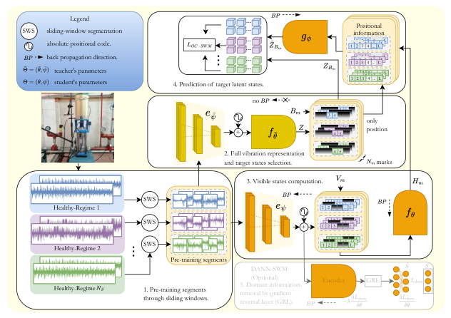
Figure 2.
Experimental platform and data acquisition system.
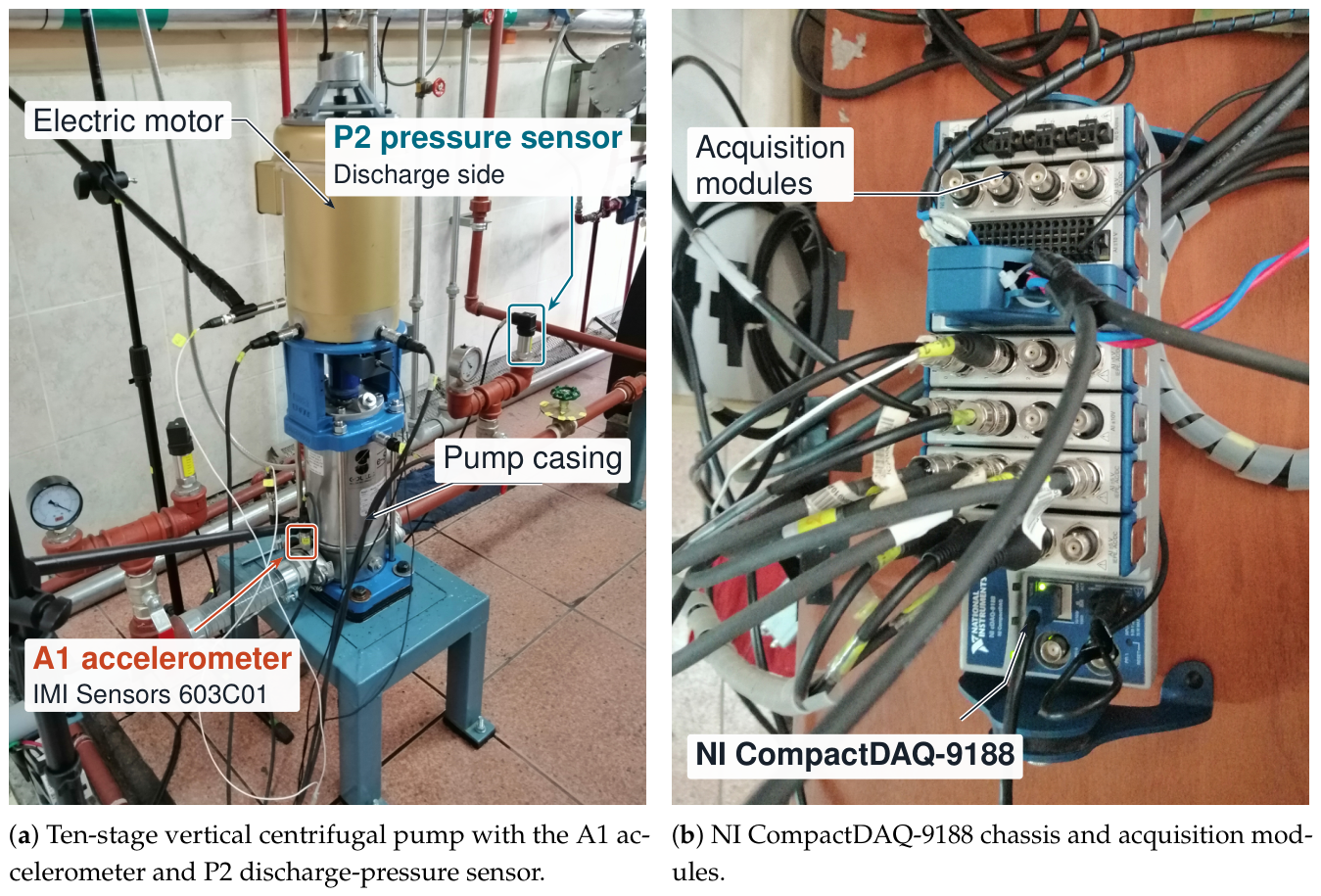
Figure 3.
Label-efficiency curves. AULC corresponds to the normalized trapezoidal area between 30 and 300 labeled training windows per class.
Figure 3.
Label-efficiency curves. AULC corresponds to the normalized trapezoidal area between 30 and 300 labeled training windows per class.
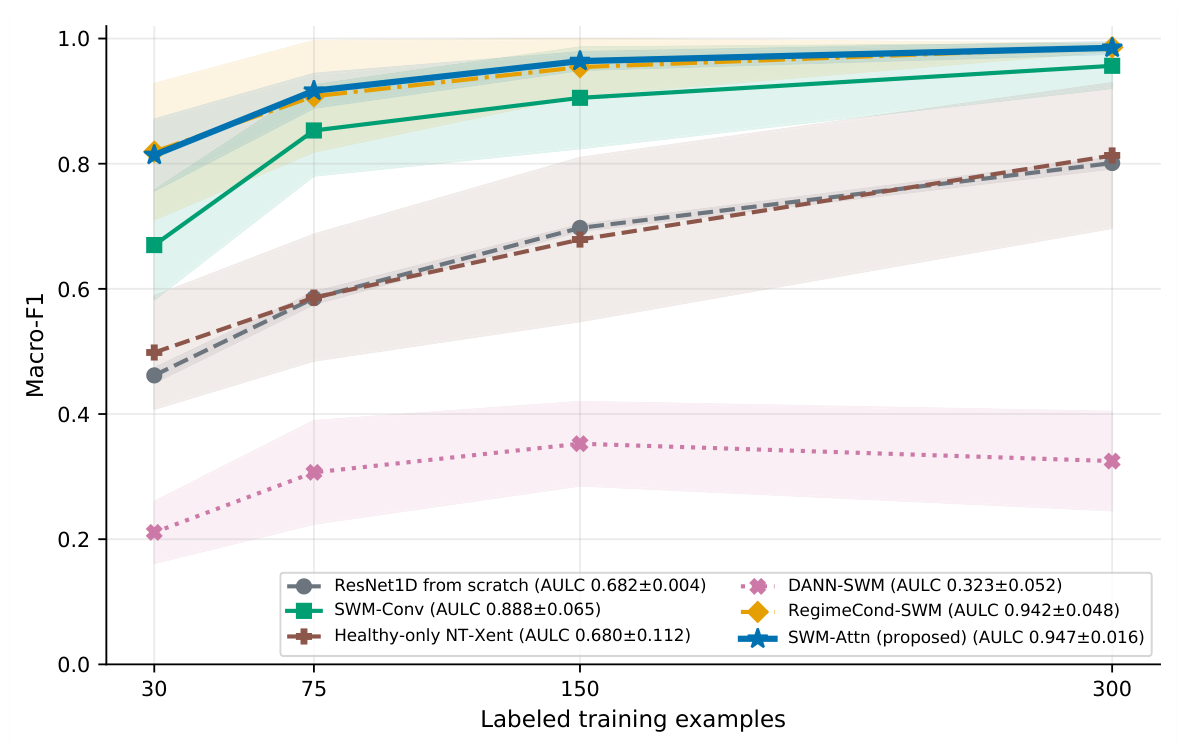
Figure 4.
Row-normalized test confusion matrices for SWM-Attn.
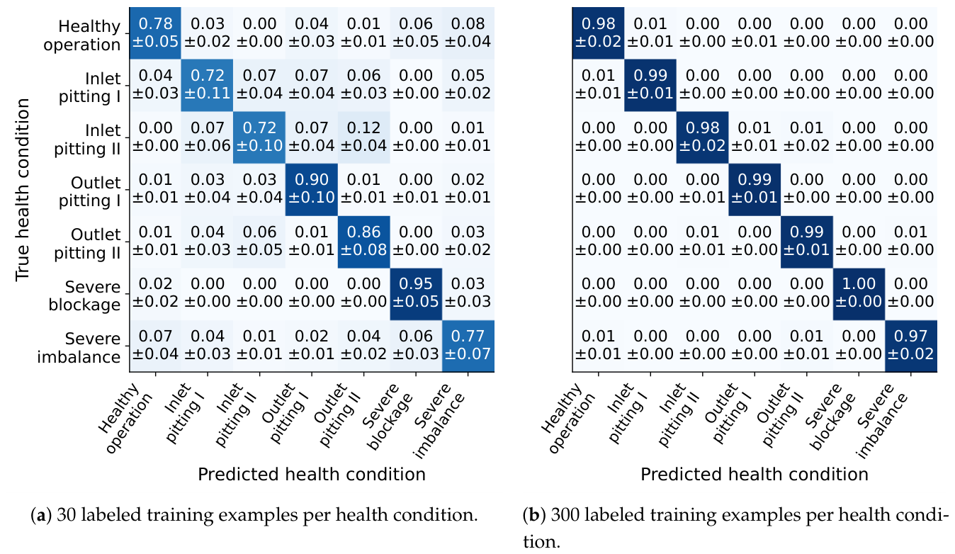
Figure 5.
Value acquired during healthy-only pretraining.
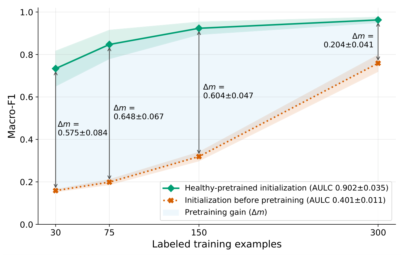
Figure 6.
Shared and unique correct decisions on the same test examples for models initialized with healthy-pretrained weights and without pretraining.
Figure 6.
Shared and unique correct decisions on the same test examples for models initialized with healthy-pretrained weights and without pretraining.
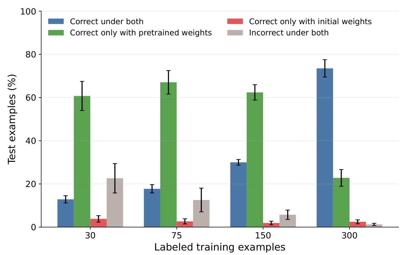
Figure 7.
Accessibility of the hydraulic state from healthy representations before supervised adaptation.
Figure 7.
Accessibility of the hydraulic state from healthy representations before supervised adaptation.
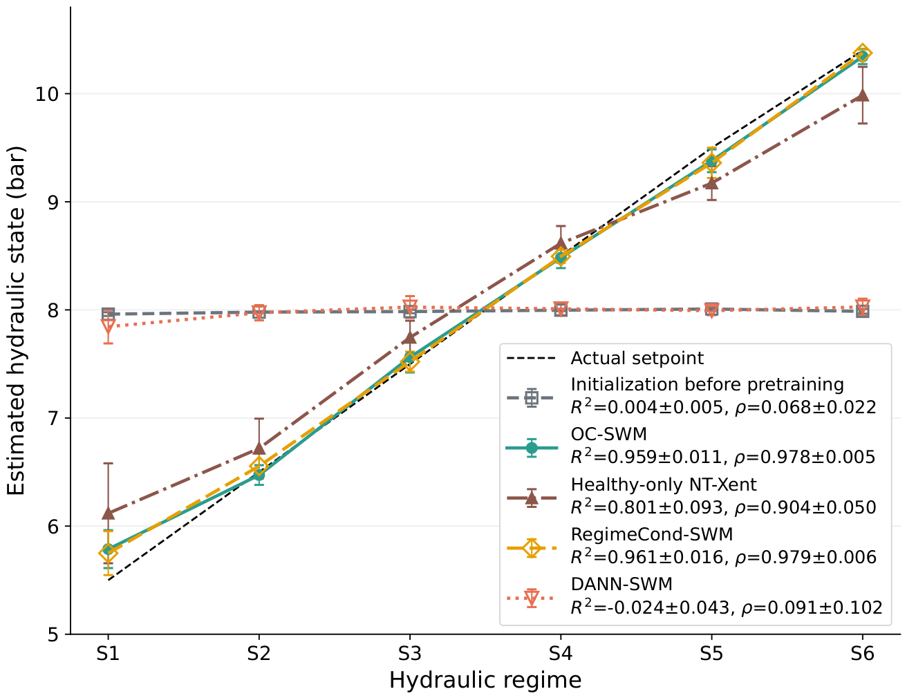

Table 1.
Diagnostic classes and physical configurations used in the study.
| Diagnostic class | Physical configuration |
|---|---|
| Healthy operation | All ten stages operate under healthy conditions. |
| Inlet pitting I | Pitting at the impeller inlet in stages 10–6, with severities of 41%, 31%, 22%, 17%, and 12% in stages 10, 9, 8, 7, and 6, respectively. |
| Inlet pitting II | Pitting at the impeller inlet in stages 10–5, with severities of 61%, 55%, 48%, 41%, 31%, and 22% in stages 10, 9, 8, 7, 6, and 5, respectively. |
| Outlet pitting I | Pitting at the impeller outlet in stages 10–6, with severities of 41%, 31%, 22%, 17%, and 12% in stages 10, 9, 8, 7, and 6, respectively. |
| Outlet pitting II | Pitting at the impeller outlet in stages 10–5, with severities of 61%, 55%, 48%, 41%, 31%, and 22% in stages 10, 9, 8, 7, 6, and 5, respectively. |
| Severe blockage | Impeller blockage in stages 10–5, with 6, 5, 4, 3, 2, and 1 blocked channels in stages 10, 9, 8, 7, 6, and 5, respectively. |
| Severe imbalance | Impeller imbalance in stages 10–5, with levels of 5.1%, 3.8%, 2.8%, 2.5%, 1.2%, and 0.3% in stages 10, 9, 8, 7, 6, and 5, respectively. |
Table 2.
Acquisition assignment across the eight evaluation folds.
| Fold | Training | Validation | Test |
|---|---|---|---|
| 1 | R6–R10 | R4–R5 | R1–R3 |
| 2 | R7–R10, R1 | R5–R6 | R2–R4 |
| 3 | R8–R10, R1–R2 | R6–R7 | R3–R5 |
| 4 | R9–R10, R1–R3 | R7–R8 | R4–R6 |
| 5 | R10, R1–R4 | R8–R9 | R5–R7 |
| 6 | R1–R5 | R9–R10 | R6–R8 |
| 7 | R2–R6 | R10, R1 | R7–R9 |
| 8 | R3–R7 | R1–R2 | R8–R10 |
Table 3.
Convolutional state encoder used for the pump.
| Layer | Channels | Kernel | Stride | Padding | Length | Receptive field |
|---|---|---|---|---|---|---|
| Conv1 | 7 | 2 | 3 | 4096 | 7 | |
| Conv2 | 7 | 2 | 3 | 2048 | 19 | |
| Conv3 | 7 | 2 | 3 | 1024 | 43 | |
| Conv4 | 7 | 2 | 3 | 512 | 91 | |
| Conv5 | 7 | 2 | 3 | 256 | 187 | |
| Conv6 (NORF) | 1 | 6 | 0 | 43 | 187 |
Table 4.
Macro-F1 of SWM-Attn under each hydraulic regime.
| Hydraulic regime | Labeled training examples per class | |||
|---|---|---|---|---|
| 30 | 75 | 150 | 300 | |
| S1 | ||||
| S2 | ||||
| S3 | ||||
| S4 | ||||
| S5 | ||||
| S6 | ||||
Table 5.
Gain from healthy-only pretraining by health condition and hydraulic regime.
| Labeled training examples | ||||
|---|---|---|---|---|
| 30 | 75 | 150 | 300 | |
| Health condition | ||||
| Healthy operation | ||||
| Inlet pitting I | ||||
| Inlet pitting II | ||||
| Outlet pitting I | ||||
| Outlet pitting II | ||||
| Severe blockage | ||||
| Severe imbalance | ||||
| Hydraulic regime | ||||
| S1 | ||||
| S2 | ||||
| S3 | ||||
| S4 | ||||
| S5 | ||||
| S6 | ||||
Table 6.
AULC of the diagnoser controls relative to SWM-Attn.
| Configuration | AULC | Difference from SWM-Attn |
|---|---|---|
| SWM-Attn | — | |
| SWM-Conv | ||
| SWM-Attn with family supervision |
Table 7.
Training cost and active diagnostic-model size with 300 labeled windows per class. The parameter count and storage consider only the modules used during diagnostic inference.
Table 7.
Training cost and active diagnostic-model size with 300 labeled windows per class. The parameter count and storage consider only the modules used during diagnostic inference.
| System | Pretraining (min) | Diagnostic training (min) | Active parameters (M) | FP32 weights (MB) |
|---|---|---|---|---|
| ResNet1D | — | 3.848 | 15.39 | |
| SWM-Conv | 0.664 | 2.66 | ||
| Healthy-only NT-Xent | 0.633 | 2.53 | ||
| DANN-SWM | 0.766 | 3.07 | ||
| RegimeCond-SWM | 0.766 | 3.06 | ||
| SWM-Attn | 0.766 | 3.06 |
Disclaimer/Publisher’s Note: The statements, opinions and data contained in all publications are solely those of the individual author(s) and contributor(s) and not of MDPI and/or the editor(s). MDPI and/or the editor(s) disclaim responsibility for any injury to people or property resulting from any ideas, methods, instructions or products referred to in the content. |
© 2026 by the authors. Licensee MDPI, Basel, Switzerland. This article is an open access article distributed under the terms and conditions of the Creative Commons Attribution (CC BY) license.
Copyright: This open access article is published under a Creative Commons CC BY 4.0 license, which permit the free download, distribution, and reuse, provided that the author and preprint are cited in any reuse.