

Submitted:
13 October 2026
Posted:
14 October 2026
You are already at the latest version
Abstract
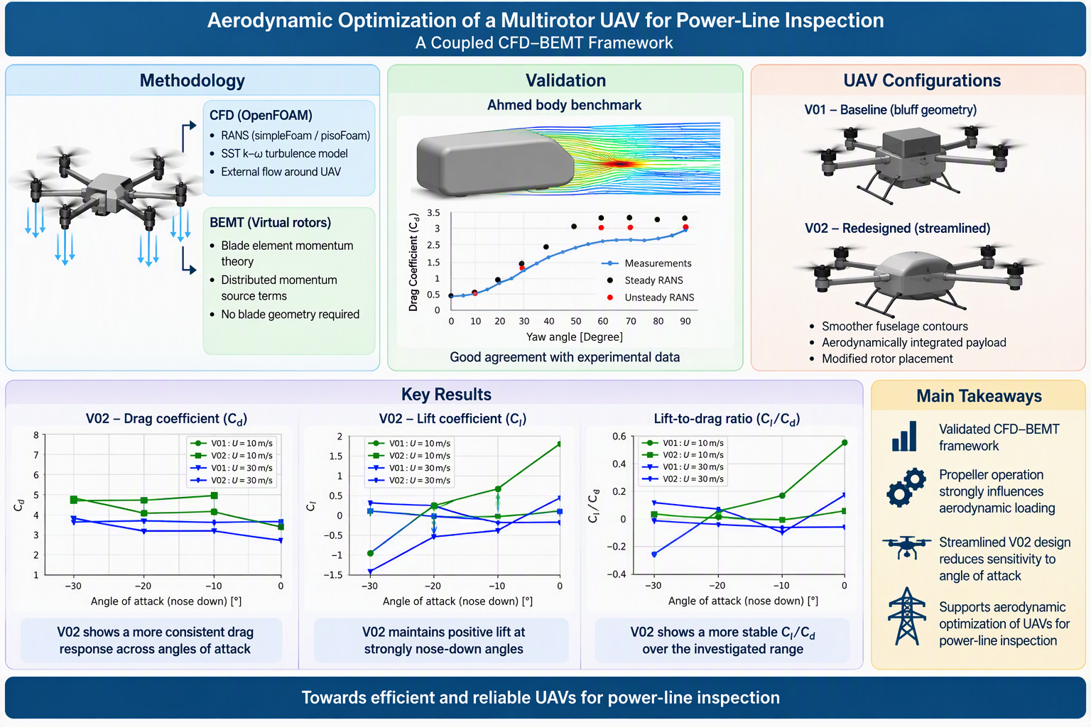
Predicting the aerodynamic performance of multirotor unmanned aerial vehicles (UAVs) remains challenging because of complex rotor–rotor and rotor–body interactions. Experimental characterisation of these interactions is often costly and time-consuming, making computational methods valuable for aerodynamic design and optimisation. This study presents a coupled computational fluid dynamics and blade element momentum theory (CFD-BEMT) framework for evaluating a multirotor UAV developed for power-line inspection. The airflow was simulated using OpenFOAM, while the propellers were represented as virtual rotors through distributed momentum-source terms calculated using BEMT. The CFD methodology was assessed by comparing predicted Ahmed-body drag coefficients at different yaw angles with experimental measurements. Steady-state Reynolds-averaged Navier–Stokes simulations provided satisfactory predictions at low yaw angles, while unsteady simulations generally improved the predictions at higher yaw angles, where large-scale flow separation and wake unsteadiness became significant. Standalone static-thrust measurements were also used as reference data to examine changes in rotor loading after integration with the UAV. The computational framework was subsequently applied to a baseline bluff-body configuration, V01, and a redesigned configuration, V02, incorporating smoother fuselage contours, improved payload integration, and modified rotor placement. A comprehensive simulation matrix was used to investigate the effects of forward velocity, propeller rotational speed, and nose-down angle of attack. The results show that propeller operation substantially modifies the aerodynamic response through nonuniform rotor-induced flow and rotor–body interactions. Compared with V01, the redesigned V02 configuration generally exhibits smaller variations in lift, drag, and lift-to-drag ratio across the investigated angles of attack. However, V02 does not provide uniformly lower drag or a consistently higher lift-to-drag ratio under all operating conditions. Its principal advantage is a more consistent aerodynamic response and reduced sensitivity to changes in nose-down angle of attack. The results demonstrate the capability of the coupled CFD-BEMT framework to assess installation effects, quantify rotor–body interactions, and support the aerodynamic development of multirotor inspection UAVs.
Keywords:
multirotor UAV
; computational fluid dynamics
; blade element momentum theory
; rotor–body interaction
; aerodynamic optimisation
; power-line inspection
; OpenFOAM
1. Introduction
Unmanned aerial vehicles (UAVs), commonly referred to as drones, have undergone substantial technological development and commercial expansion over the past many decades. Although UAV technology was initially driven largely by military and defence applications, advances in propulsion systems, sensing, navigation, communication, automation, and data processing have enabled its widespread adoption in civilian and industrial sectors. UAVs are particularly attractive for operations in remote, hazardous, or difficult-to-access environments, where conventional inspection and data-acquisition methods may expose personnel to safety risks or require considerable time and resources.
The versatility of UAV technology has led to the development of a broad range of vehicle sizes, configurations, payload capacities, and operational capabilities. UAVs are now employed in agriculture, construction, surveying, offshore energy, oil and gas, infrastructure inspection, cinematography, environmental monitoring, emergency response, medical logistics, transportation, and industrial-plant inspection. Within the energy sector, UAVs are increasingly considered for inspecting pipelines, wind turbines, solar installations, and electrical transmission infrastructure. Their ability to carry optical, thermal, and other specialised sensors enables high-resolution data acquisition while reducing the need for personnel to access hazardous locations directly.
Power-line inspection represents a particularly demanding UAV application because the vehicle may be required to travel long distances, maintain stable flight in variable atmospheric conditions, operate close to electrical infrastructure, and carry multiple inspection sensors. These requirements place considerable demands on flight endurance, range, payload capacity, stability, and energy efficiency. The aerodynamic performance of the vehicle is therefore a critical design consideration. Excessive aerodynamic drag increases propulsion-power requirements and can reduce operational range, whereas unfavourable aerodynamic loading and strong rotor-body interactions may adversely affect vehicle stability and control.
The wide diversity of UAV applications has consequently encouraged the development of application-specific airframes rather than universally applicable configurations. For long-range inspection missions, the UAV geometry, rotor arrangement, payload integration, and operating conditions must be considered as an interconnected aerodynamic system. A vehicle designed primarily around packaging and payload constraints may contain bluff components, abrupt geometric transitions, and unfavourable rotor locations that introduce flow separation and wake interference. Aerodynamic analysis and optimisation are therefore required during the design process to improve vehicle performance and ensure that the selected configuration is suitable for its intended operational environment.
Comprehensive reviews have documented the broad diversity of UAV configurations and their expanding range of applications. Hassanalian and Abdelkefi [1] classified different types of aerial vehicles, ranging from conventional unmanned aircraft to highly miniaturised systems such as smart dust, and discussed their associated applications and design challenges. In addition, Gonzalez et al. [2] and Floreano et al. [3] provided extensive overviews of UAV technologies, with particular emphasis on the capabilities and future potential of small-scale aerial vehicles.
Sevendof AS (https://www.sevendof.com/) is developing UAVs specifically for power-line inspection. Such applications require the vehicle to cover long distances while maintaining low energy consumption, adequate payload capacity, and stable operation under variable environmental conditions. The design of these UAVs therefore requires the simultaneous consideration of vehicle geometry, payload integration, rotor arrangement, operating conditions, and mission requirements. Among these factors, aerodynamic performance is particularly important because excessive drag increases the propulsion-power requirement and reduces the achievable range and endurance. Unfavourable aerodynamic loading may also introduce stability and control challenges. Aerodynamic characterisation and optimisation should therefore be incorporated into the UAV design process from an early stage.
Full-scale aerodynamic characterisation using wind-tunnel testing or other experimental techniques can be prohibitively expensive and time-consuming, particularly for companies developing specialised UAV solutions in which multiple design iterations must be evaluated. Furthermore, modifications to the airframe, payload arrangement, or rotor locations may require new experimental models and repeated testing. Numerical aerodynamic analysis provides a more practical means of screening alternative configurations before constructing physical prototypes. When supported by appropriate validation, computational methods can reduce the number of required experiments, shorten the design cycle, and provide detailed information about pressure distributions, wake structures, flow separation, and rotor-body interactions that may be difficult to obtain experimentally.
Although the aerodynamics of conventional aircraft and helicopters have been studied extensively, comparatively fewer investigations have addressed the coupled aerodynamic behaviour of multirotor UAVs. Many existing studies concentrate on isolated rotors or simplified rotor arrangements to examine rotor-rotor interactions, wake development, and static-thrust performance. Such investigations are valuable for propeller selection and propulsion-system characterisation, but they do not fully represent the aerodynamic environment experienced by rotors integrated into a complete vehicle. In particular, rotor-body interactions can modify the local inflow, pressure distribution, wake trajectory, and aerodynamic loading of both the rotors and the airframe. Previous investigations of multicopter aerodynamics have considered several relevant design aspects, including blade geometry, as examined by Siddhardha [4], the integration of fixed wings, as investigated by Chipade et al.[5]; and the analysis of in-flight force signals, as reported by Esakki et al.[6].
The design of many multirotor UAV configurations continues to rely on empirical models, small-scale experiments, field testing, and engineering experience. Field experiments provide representative operational conditions but are affected by difficulties in controlling atmospheric parameters, establishing suitable test infrastructure, operating complex measurement systems, and ensuring repeatability. These practical requirements can also result in considerable time and cost [7]. Wind-tunnel testing provides a more controlled experimental environment and can reproduce selected operating and ambient conditions [8]. Nevertheless, the construction of representative models, integration of rotating propulsion systems, and measurement of unsteady aerodynamic loads remain technically demanding and expensive. Consequently, experimental assessment alone may restrict the number of design alternatives that can be considered. A more detailed understanding of rotor-body interactions could support the development of optimised configurations with improved endurance, range, payload capacity, and forward-flight performance[9,10].
Aerodynamic methods developed for conventional fixed-wing aircraft and single-rotor helicopters cannot always be applied directly to small multirotor UAVs. One important distinction is the Reynolds-number range in which these vehicles operate. Small UAVs commonly operate at relatively low Reynolds numbers, where viscous effects become more significant relative to inertial effects and can strongly influence boundary-layer development, flow separation, and aerodynamic loading. Accordingly, rotor models and aerodynamic correlations developed for larger aircraft operating at substantially higher Reynolds numbers may require modification or additional validation before being applied to small UAVs. Multirotor configurations introduce further complexity because neighbouring rotors and the vehicle body are positioned in close proximity, resulting in strong rotor-rotor and rotor-body interactions [9,10]]. These studies [9,10] demonstrated that the separation distance between adjacent or counter-rotating propellers significantly affects wake development and the surrounding flow field, thereby influencing the aerodynamic performance of the complete vehicle.
The increasing use of UAVs has consequently motivated several numerical and experimental studies aimed at characterising propeller-induced flow and its influence on vehicle performance. Paz et al. [7] conducted a CFD investigation of quadcopter stability in proximity to walls and the ground, demonstrating the importance of interactions between the rotor-induced flow and nearby surfaces. Hakjin Lee and Duck-Joo Lee [11] numerically investigated a quadcopter under hover conditions to examine the effects of mutual rotor interaction on aerodynamic performance, wake structures, and acoustic pressure levels. Their methodology combined a nonlinear vortex-lattice method, a vortex-particle method, and an acoustic analogy based on Farassat’s formulation. The simulations showed that the wakes and induced flow structures generated by the rotors were drawn radially towards the centre of the vehicle because of the influence of adjacent rotors. This behaviour resulted in strong wake-to-wake interactions and the formation of asymmetric wake structures. Lee et al. [11] also applied a modified free-wake method to analyse multirotor aerodynamic performance. Their approach employed a time-marching free-wake formulation combined with a source-doublet panel method to represent the vehicle surfaces and the evolving rotor wakes. Yoon et al. [12] investigated the influence of separation distances between neighbouring rotors and between the propulsion system, fuselage, and lifting surfaces. Their results indicated that reducing the distance between adjacent rotors can decrease the aerodynamic efficiency of a quadrotor system.
Collectively, these studies demonstrate that rotating propellers have a substantial influence on UAV aerodynamic performance. Shukla et al. [9,10] conducted detailed experimental investigations of several in-plane multirotor arrangements. Their results showed that side-by-side rotor experiments provide valuable information regarding aerodynamic interactions relevant to a broad range of in-plane rotor configurations. High-speed stereoscopic particle-image velocimetry was employed to resolve the velocity field and capture the development and interaction of the rotor wakes. These investigations highlighted the strong dependence of wake structure and rotor performance on rotor spacing and relative placement.
Propeller performance is commonly characterised using static-thrust measurements. Although such measurements provide useful information about the performance of isolated or coaxial propellers, they generally do not account for interactions with the UAV fuselage, support arms, payload module, or neighbouring rotor wakes. Consequently, the thrust generated by a propeller after installation on the vehicle can differ from its standalone static-thrust value. Dynamic testing can provide a more representative assessment but requires specialised infrastructure and is generally more complex and costly than static testing. Both static and dynamic measurements can therefore become time-consuming when numerous propeller arrangements, rotational speeds, flight velocities, and vehicle geometries must be evaluated. A validated numerical methodology capable of reproducing the principal installation effects could replace a substantial proportion of these physical tests while enabling a wider design space to be investigated.
Several modelling approaches have been developed to estimate propeller performance. Simplified formulations can estimate thrust from quantities such as the inflow velocity, thrust coefficient, propeller diameter, and rotational speed. However, these formulations may not adequately represent rotor drag, nonuniform inflow, or rotor-airframe interactions during forward flight [13]. Hoffmann et al. [14] proposed an alternative approach that requires the mechanical power delivered to each propeller to be known. In practical applications, this method requires current measurements for individual motors and an accurate model relating electrical input to mechanical output. The additional current-sensing equipment may increase the mass and complexity of the onboard electronics, while uncertainties in the electrical-to-mechanical efficiency model can affect the accuracy of the estimated rotor forces [15].
Blade element theory (BET) has been applied to overcome some of the limitations of purely empirical and measurement-based methods for estimating propeller performance [16,17]. BET divides a propeller blade into radial elements and determines the aerodynamic forces acting on each element from the local blade geometry and flow conditions. The method has subsequently been combined with momentum theory to form blade element momentum theory (BEMT), which couples the local blade loading with the induced velocity through the rotor disk. BEMT formulations have been applied to predict rotor thrust during hover and axial climb, often using simplifying assumptions regarding the inflow and blade incidence. However, their accuracy can decrease during forward flight, particularly when the rotor experiences nonuniform and asymmetric inflow.
Gill and D’Andrea [15] proposed a propeller model for estimating thrust, drag, and torque over operating conditions ranging from hover to high-speed forward flight. Their formulation incorporated both Blade Element Theory (BET) and Blade Element Momentum Theory (BEMT) and was applied to three different propeller geometries to assess its generality and predictive capability. Their analysis identified limitations in conventional blade-element formulations under high-speed conditions, particularly in representing the distribution of induced aerodynamic effects along the blade. On this basis, modifications were proposed to improve the prediction of propeller forces during forward flight.
To address the limitations of isolated propeller models and computationally expensive blade-resolved CFD simulations, a coupled CFD-BEMT approach for representing single and counter-rotating propellers was developed based on the formulation of Patrao [18] and validated in our previous publication [19]. In this approach, the aerodynamic influence of each propeller is calculated using BEMT and introduced into the CFD governing equations through distributed momentum-source terms within predefined rotor regions. The surrounding flow, including interactions among the propellers, UAV body, payload module, and support structures, is resolved using CFD. This formulation eliminates the need to represent and mesh the detailed rotating blade geometry, thereby reducing the computational effort required to investigate multiple vehicle configurations and operating conditions.
In the present study, the numerical methodology is evaluated in two stages before being applied to the aerodynamic optimisation of the multirotor UAV. First, the CFD setup is assessed against experimental drag-coefficient data for the Ahmed body at different yaw angles. This benchmark is used to evaluate the computational-domain dimensions, grid sensitivity, boundary conditions, near-wall treatment, turbulence modelling, and the suitability of steady and unsteady solver formulations. Second, the thrust predicted for the propellers under installed conditions is compared with standalone static-thrust data to quantify the influence of rotor integration and the nonuniform flow generated by the vehicle. The resulting CFD-BEMT framework is then applied to two UAV configurations to investigate the effects of forward velocity, propeller rotational speed, and angle of attack on the aerodynamic coefficients. The primary objective is to determine how modifications to the fuselage geometry, payload integration, and rotor arrangement affect the aerodynamic response and its sensitivity to operating conditions.
2. Materials and Methods
In the present study, a coupled computational fluid dynamics and blade element momentum theory (CFD-BEMT) framework was employed to investigate the aerodynamic behaviour of two multirotor UAV configurations. Before its application to the UAV analysis, the CFD methodology was evaluated using the Ahmed body as a benchmark bluff-body geometry. Steady-state and transient simulations were performed using the OpenFOAM solvers simpleFoam and pisoFoam, respectively.
The benchmark study was used to assess and select the principal numerical settings required for the UAV simulations, including the computational-domain dimensions, mesh resolution, boundary conditions, inflow parameters, near-wall treatment, turbulence model, spatial discretisation schemes, pressure-velocity coupling, convergence criteria, and solver formulation. The performance of steady-state and transient approaches was also examined under flow conditions involving different degrees of separation and wake unsteadiness.
Based on the benchmark results, an appropriate combination of numerical accuracy, stability, and computational efficiency was selected. The resulting computational methodology was subsequently applied to calculate the lift and drag coefficients of the baseline V01 and redesigned V02 UAV configurations over the investigated ranges of forward velocity, propeller rotational speed, and angle of attack. The BEMT-based virtual-rotor model was coupled with the CFD solver to represent propeller-induced flow without explicitly resolving the rotating blade geometry.
CFD-BEMT: A numerical approach for modeling the multirotor UAV
OpenFOAM (https://openfoam.org/) is an open-source computational fluid dynamics (CFD) software package used to simulate a wide range of compressible and incompressible flow problems. In the present study, OpenFOAM was employed to investigate the aerodynamic performance of a multirotor UAV under conditions both with and without propeller operation. Within a CFD framework, propellers can generally be represented using either a direct or an indirect modelling approach.
In the direct approach, the complete propeller geometry is explicitly resolved within the computational mesh, and its rotation is represented using techniques such as dynamic meshes, sliding interfaces, or rotating reference frames. This approach enables a detailed representation of the propeller-blade surfaces and the associated flow structures, including blade-tip vortices and transient rotor-wake behaviour. However, it requires the detailed propeller geometry to be imported into the CFD pre-processing environment and accurately discretised. The resulting mesh must provide sufficient resolution around the blades and within the rotor wake, making the procedure computationally expensive and time-consuming. These requirements limit the practicality of the direct approach for UAV design and optimisation studies, in which a large number of configurations and operating conditions must be evaluated.
The indirect approach addresses these limitations by replacing the explicitly resolved propeller blades with a virtual mathematical representation of the rotor. In this approach, the aerodynamic influence of the propeller is introduced into the governing flow equations through distributed body-force source terms calculated from the propeller geometry and operating conditions. Eliminating the need to mesh the individual propeller blades substantially reduces both the computational cost and the manual effort required to prepare each simulation. Consequently, multiple UAV configurations and operating conditions can be analysed within a practical design and optimisation process.
In the present study, the indirect propeller model was implemented by coupling the CFD solver with a blade element momentum theory (BEMT) model. The BEMT model calculates the aerodynamic forces generated by the propeller, which are then introduced as momentum source terms within predefined rotor regions in the OpenFOAM computational domain. This coupled CFD-BEMT approach represents the principal aerodynamic effects of the propellers while retaining the computational efficiency required for systematic UAV design and optimisation. A detailed description of the mathematical formulation, numerical implementation, and validation of the virtual propeller model is provided in our previous publication [19].
OpenFOAM solves generalized Navier–Stokes (NS) equation in which fundamental conservation equations; of mass and momentum are solved using Finite Volume Method (FVM).
The continuity equation or conservation of mass is:
The momentum equation is:

where the averaged stress tensor, τ¯¯¯, for Newtonian fluids is given by:
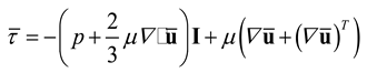
R, is the Reynolds stress tensor

Only the anisotropic contribution of the Reynolds stress tensor transports momentum, whereby the isotropic contribution can be added to the mean pressure, leading to the full form:

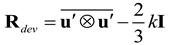
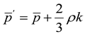
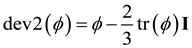
Where ρ is the density of the medium, is the velocity vector, g is the gravitational force, is the averaged stress tensor, and R is the Reynolds stress tensor. Si is the source term to represent the propeller dynamic. Si is the source term to replace the actual geometry of the propeller blades by lines carrying body forces corresponding to the loading of the propeller blades. With this approach, it is not necessary to make a detailed mesh for the propeller geometry which will otherwise become computationally demanding. A detailed implementation of this approach has been given in our previous publication [19]. The effect of the propeller on the flow is introduced via source terms Si to the governing equations (see Equation-2) for the cells in the mesh that are located inside a predefined propeller zone. These zones are predefined using the OpenFOAM meshing option. The implementation procedure is explained in our previous publication [19].
Turbulent flows are commonly simulated using two principal approaches: Reynolds-averaged Navier–Stokes (RANS) modelling and large-eddy simulation (LES). LES resolves the large, energy-containing turbulent structures while modelling the smaller, subgrid-scale motions. Although this approach can provide detailed information about transient flow structures, its computational cost remains substantial, particularly for high-Reynolds-number flows, complex geometries, and simulations requiring adequate near-wall resolution. RANS methods instead solve the time-averaged governing equations and model the effects of turbulence on the mean flow. Owing to their favourable balance between computational cost and predictive capability, RANS methods remain widely used for engineering applications and were therefore adopted in the present study.
The accuracy of a RANS simulation depends strongly on the selection of an appropriate turbulence model, particularly for multirotor UAV flows involving adverse pressure gradients, boundary-layer separation, rotor-induced turbulence, and rotor-body wake interactions. In the present study, turbulence was modelled using the shear-stress transport (SST) k-ω model. This model combines the robust near-wall formulation of the standard k-ω model with the reduced free-stream sensitivity associated with the k-ε model. The k-ω formulation is applied in the near-wall region, where it provides an effective representation of boundary-layer development and wall shear stress. Away from solid surfaces, the model gradually transitions towards a k-ε-type formulation, which is less sensitive to prescribed free-stream turbulence quantities.
The transition between the two formulations is controlled by blending functions, allowing the SST k-ω model to retain the advantages of each approach in the appropriate regions of the flow. In addition, the model incorporates a limiter on the turbulent shear stress, which improves its performance in flows involving adverse pressure gradients and separation. These characteristics make the SST k-ω model suitable for the present application, in which the airflow around the UAV is influenced by complex geometry, boundary-layer separation, propeller-induced flow, and interactions between the rotor wakes and the vehicle body[20]. In the SST k-omega turbulence model, besides continuity and momentum equations, a transport equation of turbulence kinetic energy and turbulence energy dissipation is also solved.
The governing equations of the model are the turbulence specific dissipation given by [21]:
and the turbulent kinetic energy is given by:
The turbulence viscosity is obtained using:
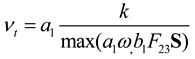
Default model coefficients taken from OpenFoam user guide (https://www.openfoam.com/documentation/)
| αk1 | αk2 | αω1 | αω2 | β1 | β2 | γ1 | γ2 | β* | a1 | b1 | c1 |
| 0.85 | 1.0 | 0.5 | 0.856 | 0.075 | 0.0828 | 5/9 | 0.44 | 0.09 | 0.31 | 1.0 | 10.0 |
Where,
In equation-9: ω is turbulence dissipation, Gω represents the generation of turbulence dissipation due to mean velocity gradients, Sω is user defined turbulence dissipation source term, u is the velocity vector, ρ is the density of the fluid, Dω represents the turbulence dissipation effective diffusivity, β is a factor used in calculating the turbulence diffusion, and Sω represents the cross-diffusion term
In equation-10: k is turbulent kinetic energy, Gk represents the generation of turbulence kinetic energy due to mean velocity gradients, Sk is user defined turbulent kinetic energy source term, u is the velocity vector, ρ is the density of the fluid, Dk represents the kinetic energy effective diffusivity, β* is a factor used in calculating the kinetic energy diffusion.
Model validation of Ahmed body
The validation of the proposed CFD-BEMT method using standalone propeller measurement data is detailed in our previous publication [19]. In the present study, the proposed CFD methodology is validated using the Ahmed body benchmark, with particular emphasis on the selection of boundary conditions, inlet-flow parameters, turbulence models, spatial discretization schemes, and computational-grid resolution. The Ahmed body is one of the most widely studied benchmark geometries in automotive aerodynamics. Its geometry consists of three principal sections: a rounded front surface that guides the incoming flow and limits premature separation, a rectangular central section that promotes flow development, and a slanted rear surface where substantial flow separation and wake formation occur.
The Ahmed body has been extensively investigated through both experimental and numerical studies and is widely regarded as a standard benchmark geometry in aerodynamic research. The high-quality experimental datasets available in the literature provide an important basis for validating numerical methods, turbulence models, mesh-refinement strategies, grid-convergence procedures, near-wall treatments, and spatial discretization schemes. Despite its relatively simple geometry, accurately predicting the airflow around the Ahmed body remains challenging because of the complex flow structures that develop around and behind it. In particular, the wake is characterised by substantial flow separation, unsteady behaviour, vortex formation, and interactions between multiple vortical structures. These phenomena contribute significantly to aerodynamic drag and make the Ahmed body a demanding test case for evaluating the predictive capabilities of CFD models.
One of the principal challenges in modelling the flow around the Ahmed body is the selection and implementation of an appropriate turbulence model. The selected model must adequately represent the boundary-layer development, flow separation, wake dynamics, and turbulence generated downstream of the body. In addition, the type and resolution of the computational mesh, the mesh-refinement strategy, and the near-wall modelling approach play important roles in determining the accuracy and reliability of the numerical results. Particular attention must be given to regions near the body surfaces and within the separated wake, where strong velocity gradients and complex vortical structures are present. The choice of spatial and temporal discretization schemes introduces an additional consideration, as these schemes must provide sufficient numerical accuracy and stability while maintaining a reasonable computational cost.
To address these modelling challenges, several CFD approaches have been applied to investigate the aerodynamic behaviour of the Ahmed body. These include Reynolds-averaged Navier–Stokes (RANS) simulations, large-eddy simulation (LES), detached-eddy simulation (DES), and implicit large-eddy simulation (ILES). Each approach offers different advantages and limitations in terms of computational cost, turbulence resolution, and the ability to capture unsteady flow separation and wake structures. RANS methods are generally computationally efficient and are therefore widely used in engineering applications, whereas LES, DES, and ILES can provide a more detailed representation of transient wake behaviour but require substantially greater computational resources. [23,24,25]. Each of these methods has distinct strengths and limitations in capturing the complex aerodynamic phenomena associated with the Ahmed body. Comparative studies employing these approaches have contributed to a better understanding of their respective predictive capabilities and limitations, thereby supporting the development of more robust and accurate aerodynamic modelling techniques [22]. A detailed description and comparison of these numerical approaches are beyond the scope of the present study. Bello-Millán et al. [22] experimentally investigated the aerodynamic behaviour of the Ahmed body over a range of yaw angles, β, from 0° to 90°. In the present study, their experimental results are used to validate the proposed CFD methodology and assess its ability to predict aerodynamic drag under different yaw conditions. Accordingly, CFD simulations of the Ahmed body are performed at several yaw angles corresponding to those investigated experimentally. The comparison between the numerical and experimental results provides a basis for evaluating the selected boundary conditions, turbulence model, computational mesh, near-wall treatment, and discretization schemes before applying the methodology to the multirotor UAV simulations.
Methodology for modelling of Ahmed body
The OpenFOAM methodology subsequently used to determine the aerodynamic coefficients of the UAV configurations was systematically validated against experimental data for the well-established Ahmed body benchmark over a range of yaw angles. The validation had two principal objectives: first, to assess the accuracy of the predicted aerodynamic coefficients and, second, to evaluate the influence of the solver formulation and key numerical parameters on the simulation results. Two OpenFOAM solvers were employed for this purpose: simpleFoam, which provides a steady-state solution of the incompressible Reynolds-averaged Navier–Stokes equations, and pisoFoam, which provides a transient solution using the Pressure-Implicit with Splitting of Operators algorithm.
The suitability of the steady and transient formulations was evaluated in relation to the flow characteristics observed at different yaw angles. At relatively low yaw angles, the flow was expected to exhibit comparatively limited large-scale unsteadiness, making a steady-state treatment potentially suitable. As the yaw angle increased, the flow became increasingly dominated by large-scale separation, vortex shedding, and transient wake behaviour. Both steady-state and transient simulations were therefore performed to assess the ability of the two formulations to reproduce the experimentally measured aerodynamic behaviour, particularly at higher yaw angles.
The governing equations were discretised using the finite-volume method implemented in OpenFOAM. The linearUpwind scheme was employed for the convective terms. This second-order upwind scheme uses local gradient information to provide improved spatial accuracy when interpolating flow variables between neighbouring cell centres and faces. The Gauss linear limited scheme was used for the gradient terms to achieve an appropriate balance among numerical accuracy, boundedness, and solution stability. The pressure equation was solved using the Geometric-Algebraic Multigrid (GAMG) solver, whereas smoothSolver was employed for the velocity and turbulence transport equations. For the transient simulations conducted using pisoFoam, a time step of 0.1 ms was selected to provide adequate temporal resolution of the unsteady flow structures.
The boundary conditions were specified to reproduce the physical conditions of the Ahmed body experiments as closely as possible. A fixed-value velocity condition was prescribed at the inlet, together with the corresponding turbulence quantities. At the outlet, a pressure-based inlet–outlet condition was applied to allow the flow to leave the computational domain while accommodating any local flow reversal. A no-slip condition was imposed on the bottom boundary to represent the ground surface, whereas slip conditions were applied to the remaining far-field boundaries to minimise their influence on the external flow around the Ahmed body.
Both linear and nonlinear eddy-viscosity turbulence models were examined to assess their influence on predictive accuracy, numerical stability, and convergence behaviour. The simulations were initialised using a uniform velocity field and prescribed inlet turbulence quantities, including turbulent kinetic energy and the relevant turbulence-dissipation variable. Convergence was evaluated using both the residuals of the governing equations and the evolution of the aerodynamic force coefficients. In addition, numerical probes were placed at selected locations within the computational domain to monitor important flow quantities and identify any persistent temporal variations.
The steady-state simulations were continued until the residuals had decreased sufficiently and the monitored aerodynamic coefficients no longer exhibited systematic variations. Because inherently unsteady flow structures can prevent a strictly steady solution at large yaw angles, the transient simulations were instead continued until a statistically stationary flow state was established. After the initial transient effects had decayed, the instantaneous drag coefficient was sampled over a physical period of 100 s and time-averaged to obtain a representative mean value. The averaging interval was selected to capture the temporal fluctuations associated with flow separation and wake dynamics while minimising the influence of short-duration variations on the reported drag coefficient.
This validation procedure provided a systematic basis for assessing the reliability of the selected OpenFOAM methodology before its application to the UAV configurations. In particular, the comparison between the steady-state and transient results enabled the influence of large-scale flow separation and unsteady wake behaviour to be evaluated at increasing yaw angles. The resulting validation also supported the selection of an appropriate numerical approach that balances predictive accuracy and computational cost for the extensive UAV simulation matrix considered in this study.
The Ahmed body geometry was constructed in ANSYS DesignModeler using the dimensions reported in the literature [22], as shown in Figure 1. A computational domain was subsequently defined around the Ahmed body to capture the principal characteristics of the external flow while minimising the influence of the domain boundaries on the numerical solution. A schematic representation of the computational domain is presented in Figure 2. The surface and volume meshes were generated using ANSYS Meshing. A face-meshing method was employed to produce a high-quality and geometrically representative surface mesh, which was subsequently used as the basis for generating the surrounding volume mesh.
The spatial resolution of the computational mesh is particularly important for accurately predicting boundary-layer development, flow separation, and downstream wake formation. The mesh was therefore locally refined near the Ahmed body surfaces and within the wake region. This refinement improved the resolution of the strong velocity and pressure gradients occurring near the body and enabled the separated shear layers and vortical structures within the wake to be captured more accurately. In addition, inflation layers were generated adjacent to the body surfaces to resolve the near-wall velocity gradients and wall shear stresses. The number, thickness, and growth rate of the inflation layers were specified to provide a gradual transition from the fine near-wall mesh to the comparatively coarser mesh in the outer region of the computational domain.
For the resulting mesh, the nondimensional wall-distance parameter, y+, was maintained within the range of 50–100. This range was consistent with the wall-function treatment adopted in the simulations and the near-wall requirements of the selected turbulence model. The wall functions were selected to ensure that the prediction of near-wall quantities, including wall shear stress and pressure gradients, remained compatible with the mesh resolution and turbulence-modelling strategy. The combined use of local refinement, near-wall inflation layers, and appropriate wall functions provided a consistent numerical framework for simulating the aerodynamic flow around the Ahmed body.
Overall, the computational-domain dimensions and meshing strategy were selected to resolve the principal aerodynamic phenomena affecting the Ahmed body, including boundary-layer development, flow separation, reattachment, wake formation, and vortex generation. This approach provided the spatial resolution required to support a reliable validation of the CFD methodology while maintaining a practical computational cost.
The flow simulations were conducted at a Reynolds number defined as . Here, U is the inlet velocity; L is the characteristic length of the Ahmed body, equal to 1.044 m; and ν is the kinematic viscosity of air (1.5 X 10⁻⁵). Because the Ahmed body experiments were performed with an inlet turbulence intensity of 1%, the same value was applied in the CFD simulations to ensure consistency between the numerical and experimental conditions. The computational domain was configured to accurately represent the aerodynamic flow around the Ahmed body. A uniform mean velocity of 10 m/s was prescribed at the inlet boundary, located on the upstream side of the computational domain.
The turbulent kinetic energy, k, and turbulence dissipation rate, ε, at the inlet were calculated using the following equations provided in the OpenFOAM user guide:
where I is the turbulence intensity, Cμ is a turbulence-model constant equal to 0.09, and l is the turbulence length scale. The turbulence length scale was defined based on the characteristic length of the Ahmed body.
The outlet boundary was positioned sufficiently far downstream of the Ahmed body to minimise its influence on the exiting flow. A zero-gradient condition was applied at the outlet, allowing the flow to leave the computational domain without introducing significant artificial reflections or disturbances. The front, back, and top boundaries of the computational domain were treated as free-slip surfaces. These boundary conditions eliminate wall-normal flow while neglecting tangential shear stresses, making them suitable for representing the far-field boundaries of an external aerodynamic flow. The bottom boundary was modelled as a no-slip wall to represent the ground surface and its influence on the aerodynamic behaviour of the Ahmed body.
A grid-convergence study was performed to assess the sensitivity of the numerical predictions to the computational-mesh resolution. The mesh was progressively refined until further refinement produced no significant change in the predicted aerodynamic quantities, particularly the drag coefficient. This grid-independence assessment ensured that the numerical results were not substantially influenced by the spatial discretisation of the computational domain.
Both linear and nonlinear eddy-viscosity turbulence models were evaluated. The linear models included the k-ω, k-ε, and SST k-ω formulations, while the nonlinear models included the Lien cubic k-ε model available in OpenFOAM. The nonlinear Lien cubic k-ε model exhibited convergence difficulties and required smaller time steps to achieve numerically stable solutions. In comparison, the SST k-ω model provided sufficiently accurate and stable predictions for the Ahmed body and was therefore selected for the subsequent simulations. The SST k-ω model is particularly suitable for bluff-body aerodynamics because it combines the near-wall performance of the k-ω model with the free-stream characteristics of the k-ε model.
To evaluate the accuracy of the numerical methodology, the drag coefficients predicted using steady-state and unsteady RANS simulations were compared with the experimental measurements reported by Bello-Millán et al. [22]. The comparison as a function of the Ahmed body yaw angle is presented in Figure 3 and provides insight into the predictive capabilities of the two numerical approaches under different flow conditions. At yaw angles below 30°, the computed drag coefficients were in close agreement with the experimental data, demonstrating that the selected CFD methodology and SST k-ω turbulence model provide reliable predictions within this range.
The steady-state RANS predictions show reasonably good agreement with the experimental measurements at low yaw angles. At 0°, the predicted drag coefficient is nearly identical to the measured value. The agreement remains acceptable at 20° and 30°, although the steady-state model slightly overpredicts the drag coefficient. Beyond 30°, the discrepancy increases considerably. For example, at a yaw angle of 40°, the steady-state RANS model predicts a drag coefficient of approximately 2.0, compared with the measured value of approximately 1.7. At 50°, the predicted drag coefficient increases to approximately 2.8, whereas the corresponding experimental value is approximately 2.0. At yaw angles between 60° and 90°, the steady-state predictions remain close to 3.0, while the measured values vary from approximately 2.2 to 2.6. These results demonstrate that the steady-state RANS approach increasingly overpredicts aerodynamic drag as the yaw angle increases beyond 30°.
The increasing discrepancy at higher yaw angles is associated with substantial changes in the flow structure around the Ahmed body. As the yaw angle increases, a larger lateral area is exposed to the incoming flow, and the effective streamwise length-to-width ratio decreases. These changes promote stronger flow separation and the formation of complex, asymmetric, and transient wake structures. Because steady-state RANS provides a time-averaged representation of the flow, the method cannot fully resolve transient phenomena such as vortex shedding, wake oscillations, and large-scale unsteady separation. Consequently, the steady-state approach becomes less reliable for predicting the drag coefficient at higher yaw angles. Nevertheless, the results indicate that steady-state RANS provides sufficiently accurate drag predictions for the Ahmed body at yaw angles up to approximately 30°, subject to the accuracy requirements of the intended application.
To investigate whether the predictions at higher yaw angles could be improved, additional unsteady RANS simulations were conducted at yaw angles of 10°, 30°, 60°, 70°, and 90°, as shown in Figure 3. At 10° and 30°, the unsteady predictions agree closely with the experimental measurements. At 60° and 70°, unsteady RANS predicts drag coefficients of approximately 2.6, compared with measured values of approximately 2.2 and 2.3, respectively. Although these results improve upon the corresponding steady-state predictions of approximately 3.0, the unsteady model continues to overpredict the experimental values. At 90°, however, the unsteady RANS prediction of approximately 2.7 is close to the measured drag coefficient of approximately 2.6, representing a substantial improvement over the steady-state prediction of approximately 3.0.
Overall, the unsteady RANS simulations provide better drag predictions than the steady-state simulations at the investigated high-yaw conditions, particularly at 90°. However, the remaining discrepancies at 60° and 70° indicate that introducing time dependence alone does not completely eliminate the modelling error. The residual differences may be associated with the turbulence modelling assumptions, mesh resolution in the separated wake, near-wall treatment, temporal resolution, or differences between the numerical and experimental conditions. Unsteady RANS simulations are also substantially more computationally demanding because the transient flow must be resolved over a sufficiently long physical time and the resulting aerodynamic forces must be time-averaged after a statistically stationary state has been reached.
For the UAV configurations considered in the present study, the operational incidence-angle range is limited to ±30∘. Within the corresponding low-angle range investigated using the Ahmed body, the steady-state RANS model provides an acceptable balance between predictive accuracy and computational cost. Steady-state RANS simulations were therefore used to calculate the aerodynamic coefficients of the UAV configurations. This approach enables the large simulation matrix required for aerodynamic design and optimisation to be completed at a practical computational cost while retaining sufficient accuracy within the selected operational range.
OpenFoam simulations of the UAV
Following validation of the computational methodology, including the boundary conditions, turbulence model, inlet-flow specification, near-wall treatment, and numerical schemes, the validated framework was applied to investigate the aerodynamic performance of a multirotor UAV developed by Sevendof AS. The initial UAV configuration, designated V01, comprises a central fuselage, propeller-support arms, landing gear, and a payload module. Its geometry was primarily defined by payload-integration and operational requirements. Figure 4 presents the V01 geometry without and with the virtual propeller regions incorporated into the computational model.
The external flow around the UAV was simulated using the OpenFOAM methodology described in the preceding sections. A computational domain was constructed around the vehicle, with its boundaries positioned sufficiently far from the UAV to minimise their influence on the predicted aerodynamic forces and wake development. The UAV geometry and computational domain were prepared using ANSYS DesignModeler, while the computational mesh was generated using ANSYS Meshing, as illustrated in Figure 5.
Computational domain, boundary conditions, and mesh-sensitivity assessment
The external airflow around the UAV was simulated by prescribing a uniform velocity at the upstream boundary of the computational domain. The inlet velocity was oriented normal to the boundary and specified according to the investigated operating condition, with values of 10, 20, or 30 m/s. These conditions represent equivalent UAV forward-flight velocities in quiescent air. For the domain- and mesh-sensitivity studies, the inlet velocity was fixed at 10 m/s.
A pressure inlet–outlet condition was applied at the downstream boundary, as shown in Figure 5. This condition allowed the flow to leave the computational domain while accommodating possible local flow reversal, thereby limiting artificial numerical disturbances at the outlet. The top, bottom, front, and back boundaries were treated as slip surfaces. These far-field boundary conditions imposed zero normal velocity and negligible tangential shear stress, thereby minimising the influence of the external boundaries and approximating an unconfined flow environment.
The flow field was described by the Reynolds-averaged Navier–Stokes equations, with turbulence represented using the SST k-ω model. This model was selected because of its established suitability for flows involving adverse pressure gradients, near-wall effects, and flow separation, all of which are relevant to the aerodynamic behaviour of the UAV. Wall functions consistent with the selected turbulence model and near-wall mesh resolution were employed.
The propellers were represented using the virtual-rotor methodology described in the preceding sections. In this formulation, the individual propeller blades were not explicitly resolved within the computational mesh. Instead, the aerodynamic loading calculated using BEMT was introduced into predefined rotor regions as distributed momentum-source terms. The coupled CFD-BEMT formulation substantially reduced the computational cost relative to blade-resolved simulations while retaining the principal effects of propeller-induced flow and rotor-body interaction.
Mesh-generation strategy
The mesh was locally refined in regions where high velocity and pressure gradients were expected, particularly near the UAV surfaces, within the virtual-propeller regions, and in the downstream wake. This refinement was introduced to resolve the principal aerodynamic flow structures and improve the prediction of lift and drag while maintaining a practical computational cost.
A gradual transition in cell size was applied between the refined near-body regions and the coarser far-field mesh. Relatively small cells were employed near the UAV surfaces and virtual-propeller regions, whereas progressively larger cells were used farther from the vehicle, where the spatial flow gradients were weaker. This mesh-distribution strategy reduced the overall number of computational cells while retaining adequate spatial resolution in the aerodynamically significant regions.
Inflation layers were generated adjacent to the UAV surfaces to represent the near-wall flow and resolve the boundary-layer gradients. For the selected mesh, the nondimensional wall-distance parameter, y+, ranged from approximately 30 to 70. Wall functions compatible with this y+range and the SST k-ω turbulence model were therefore employed. This near-wall treatment enabled wall shear stress and boundary-layer behaviour to be represented without fully resolving the viscous sublayer.
Convergence assessment
The iterative convergence of each simulation was evaluated using the residuals of the continuity, momentum, and turbulence-transport equations. Numerical probes were also positioned at selected locations within the computational domain to monitor relevant flow quantities, including velocity and pressure. In addition, the aerodynamic force coefficients were monitored throughout the solution process to identify any remaining systematic variations.
A simulation was considered converged when the equation residuals satisfied the prescribed convergence criteria and the monitored flow variables and aerodynamic coefficients reached stable values. This convergence procedure provided a consistent basis for evaluating the aerodynamic performance of the UAV over the investigated vehicle geometries, forward velocities, propeller rotational speeds, and angles of attack.
Computational-domain sensitivity
The sensitivity of the numerical predictions to the domain dimensions was assessed using three computational domains, designated large, medium, and small. A relatively large domain was initially considered to minimise blockage and boundary effects and to ensure that the principal flow structures were adequately captured. The domain dimensions were subsequently reduced to identify the smallest domain that produced aerodynamic coefficients sufficiently close to those obtained using the larger domains.
The domain-sensitivity study was performed at an inlet velocity of 10 m/s under both stationary-propeller and 1000-RPM conditions. The results are presented in Table 1.
Under stationary-propeller conditions, reducing the domain from the large to the small configuration changed CDfrom 3.08 to 2.94, corresponding to a relative difference of approximately 4.5%. The difference between the medium and small domains was approximately 1.0%.
With the propellers operating at 1000 RPM, CDdecreased from 3.85 for the large domain to 3.60 for the small domain, corresponding to a difference of approximately 6.5%. However, the difference between the medium and small domains was approximately 2.7%. These results indicate that the predicted drag coefficient became progressively less sensitive to further reductions in the domain dimensions.
Because the small domain produced values close to those obtained with the medium domain while requiring fewer computational resources, it was selected for the subsequent UAV simulations. The remaining difference relative to the large domain was considered acceptable for the comparative design assessment conducted in this study.
Mesh-sensitivity assessment
A mesh-sensitivity study was performed using grids containing approximately 3.20 million, 4.80 million, and 6.44 million cells. These grids were classified as coarse, medium, and fine, respectively. The study was conducted using the selected computational domain at an inlet velocity of 10 m/s under stationary-propeller and 1000-RPM conditions. The results are summarised in Table 2.
Under stationary-propeller conditions, CDdecreased from 3.10 on the coarse mesh to 2.94 on the fine mesh, corresponding to a maximum variation of approximately 5.2%. The difference between the medium and fine meshes was approximately 1.0%, indicating limited sensitivity to further mesh refinement beyond 4.80 million cells.
At 1000 RPM, the drag coefficient decreased from 3.70 on the coarse mesh to 3.50 on the fine mesh, corresponding to a maximum variation of approximately 5.4% when referenced to the coarse-mesh result. The difference between the medium and fine meshes was approximately 2.8%.
The medium mesh therefore reproduced the fine-mesh result within approximately 1.0% under stationary-propeller conditions and 2.8% at 1000 RPM. On this basis, the 4.80-million-cell mesh was selected for the remaining simulations as an appropriate compromise between numerical accuracy and computational efficiency.
Results and discussions
Thrust comparison of the propeller
The thrust generated by each of the eight propellers at 2000 RPM under installed conditions was compared with the corresponding static thrust measured for the standalone propellers [19]. The standalone measurements provide a reference for evaluating the influence of the UAV body, rotor placement, and rotor-rotor interactions on the installed thrust distribution. The comparison is presented in Table 3.
The results demonstrate that installation of the propellers on the UAV produces a nonuniform redistribution of thrust rather than a systematic reduction across all rotors. Among the upper rotors, Rotors 1 and 3 each generate 36 N, corresponding to a reduction of approximately 14.3% relative to the standalone value of 42 N. Rotors 2 and 4 generate 40 N, representing a smaller reduction of approximately 4.8%. The upper rotor pair located at the rear of the vehicle therefore experiences a larger installed-thrust penalty than the corresponding front pair. The total thrust generated by the four upper rotors decreases from a standalone reference value of 168 N to an installed value of 152 N, equivalent to an overall reduction of approximately 9.5%.
A different response is observed for the lower rotors. Rotors 5 and 7 generate 23 N and 24 N, respectively, corresponding to reductions of 8.0% and 4.0% relative to the standalone value of 25 N. In contrast, Rotors 6 and 8 generate 31 N and 33 N, representing increases of 24.0% and 32.0%, respectively. The total thrust of the lower rotor group therefore increases from 100 N under standalone conditions to 111 N under installed conditions, corresponding to an increase of 11.0%. When all eight rotors are considered collectively, the total thrust decreases only slightly, from 268 N to 263 N, equivalent to an overall reduction of approximately 1.9%. The principal installation effect is therefore not a substantial loss of total thrust, but a marked redistribution of aerodynamic loading among the individual rotors.
Figure 6 presents the pressure distribution on a plane intersecting the lower rotor locations, Rotors 5–8. The contours indicate that the inflow to Rotors 6 and 8 is influenced by both the upper rotors and the UAV body. This disturbed aerodynamic environment is consistent with the substantial deviation of their installed thrust from the standalone reference value. However, because the calculated thrust of Rotors 6 and 8 is higher rather than lower, the pressure contours should be interpreted as evidence of strong flow interaction and altered loading, not as direct evidence of thrust degradation.
The approximately symmetric thrust values obtained for the left and right upper rotors indicate that the numerical model preserves the expected lateral symmetry of the vehicle. Rotors 1 and 3 both generate 36 N, while Rotors 2 and 4 both generate 40 N. The lower rotor system exhibits a similar left-right tendency, although the corresponding values are not identical. Rotors 5 and 7 generate 23 N and 24 N, respectively, whereas Rotors 6 and 8 generate 31 N and 33 N. These differences may arise from geometric asymmetries, local variations in the rotor inflow, or differences in the interaction between the rotor disks and the surrounding vehicle components.
The observed redistribution of thrust can be attributed to the highly nonuniform inflow generated by the combined effects of the fuselage, support arms, coaxial rotor arrangement, and neighbouring rotor wakes. Under installed conditions, each rotor operates within a local aerodynamic environment that differs from the nominally undisturbed inflow of the standalone test. Depending on rotor position, the local flow may contain velocity deficits, accelerated regions, swirl, increased turbulence, and pressure gradients induced by the vehicle body and adjacent rotors. These effects modify the axial and tangential velocity components across the rotor disk and consequently alter the aerodynamic loading predicted by the BEMT model.
The reduction in thrust observed for Rotors 1, 3, 5, and 7 indicates that these rotors operate under less favourable inflow conditions than in the standalone configuration. By contrast, the increased thrust calculated for Rotors 6 and 8 suggests locally enhanced aerodynamic loading. This increase should not be interpreted as evidence that these rotors experience weaker interaction effects. Instead, the result indicates that the altered local velocity field and pressure distribution increase the thrust predicted by the coupled CFD-BEMT formulation at these rotor locations. Depending on the direction and magnitude of the induced velocity, wake interaction can either reduce or increase rotor loading.
Overall, the results demonstrate that standalone static-thrust measurements alone are insufficient to characterise the performance of individual rotors after integration into a multirotor vehicle. Although the total installed thrust differs from the summed standalone value by only approximately 1.9%, the individual rotor deviations range from a reduction of 14.3% to an increase of 32.0%. This pronounced thrust imbalance may influence vehicle trim, motor loading, power consumption, control allocation, and propulsion-system durability. The results therefore highlight the importance of accounting for rotor-body and rotor-rotor interactions when determining rotor placement and designing the propulsion and control systems of multirotor UAVs.
Aerodynamic performance of the vehicle
The aerodynamic forces acting on the UAV are governed by the fluid properties, vehicle geometry, attitude, and velocity relative to the surrounding air. The drag and lift forces can be expressed in nondimensional form as
where FDand FLdenote the drag and lift forces, respectively; ρis the air density; Uis the UAV velocity relative to the surrounding air; Srefis the reference area; and CDand CLare the nondimensional drag and lift coefficients, respectively. The same reference area was used in all simulations to enable a consistent comparison among the investigated operating conditions and UAV configurations.
A parametric CFD study was conducted to quantify the aerodynamic performance of the V01 configuration over the investigated operating envelope. Three principal parameters were varied systematically: UAV forward velocity, propeller rotational speed, and angle of attack. The forward velocity was evaluated at 10, 20, and 30 m/s, while nose-down angles of attack of 0∘, −10∘, −20∘, and −30∘were considered. The propeller rotational speeds investigated were 0, 1000, and 2000 RPM. The condition of 0 RPM represents the baseline aerodynamic response of the UAV without propeller-induced flow, whereas the rotating-propeller cases were used to quantify the influence of rotor-body and rotor-rotor interactions on the aerodynamic coefficients.
A full-factorial simulation matrix was employed, comprising three forward velocities, four angles of attack, and three propeller rotational speeds. This resulted in a total of 36 operating conditions for each UAV configuration:
Ncases = 3 velocities × 4 angles of attack × 3 rotational speeds = 36.
This systematic variation of the operating parameters enabled both their individual effects and their combined influence on CDand CLto be assessed. The stationary-propeller simulations established the aerodynamic characteristics associated with the UAV geometry alone. The rotating-propeller simulations additionally accounted for the modification of the local velocity and pressure fields caused by the rotor-induced flow. Comparison of these conditions therefore enabled the contribution of propeller operation to the overall aerodynamic loading to be distinguished from the contribution of the vehicle geometry.
The selected range of negative angles of attack represents progressively increasing nose-down attitudes during forward flight. These conditions were examined to determine how vehicle inclination modifies the projected frontal area, surface-pressure distribution, flow separation, and wake structure. The forward velocities of 10–30 m/s represent the investigated forward-flight conditions and were selected to quantify the effect of dynamic pressure on the aerodynamic forces and coefficients. Because the lowest simulated forward velocity was 10 m/s, the simulation matrix characterises forward flight rather than hover.
The complete simulation matrix is summarised in Table 4. The same matrix was subsequently applied to the V02 configuration, enabling a direct comparison between the baseline and aerodynamically modified designs under identical operating conditions. This consistent parameterisation provides a quantitative basis for evaluating the influence of fuselage geometry and propeller-induced flow on UAV aerodynamic performance.
Although stationary-propeller conditions do not represent the normal powered operation of the multirotor UAV, they provide an important aerodynamic baseline for isolating the influence of the vehicle geometry from propeller-induced flow effects. Figure 7 presents the drag and lift coefficients of the V01 configuration with the propellers stationary at forward velocities of 10, 20, and 30 m/s and angles of attack ranging from 0∘to −30∘. Although stationary-propeller conditions do not represent the normal powered operation of the UAV, they provide a useful aerodynamic baseline for isolating the influence of the V01 airframe geometry from propeller-induced flow. As shown in Figure 7, the drag coefficient increases progressively as the vehicle adopts a more negative, nose-down angle of attack. This trend is consistent across the investigated forward velocities and is attributed to the change in projected area and the associated redistribution of pressure over the fuselage, payload module, support arms, and landing gear. The increasingly nose-down orientation may also promote stronger flow separation around the bluff components of the V01 configuration, thereby increasing the pressure-drag contribution.
The lift coefficient exhibits the opposite trend, decreasing systematically as the angle of attack becomes more negative. A slightly positive lift coefficient is obtained at zero angle of attack, whereas increasingly negative values occur as the UAV is inclined further nose-down. The change in sign indicates a reversal in the direction of the vertical aerodynamic force. This behaviour reflects the progressive redistribution of pressure between the upper and lower surfaces of the vehicle as its orientation relative to the incoming flow changes.
For a fixed angle of attack, the drag and lift coefficients remain nearly invariant over the investigated range of forward velocities. The drag coefficient exhibits only a small reduction with increasing velocity, while the variation in the lift coefficient is negligible. This limited velocity dependence indicates that the principal nondimensional flow characteristics, including the overall pressure distribution and separation behaviour, remain broadly similar across the considered Reynolds-number range.
The results therefore demonstrate that the stationary-propeller aerodynamic response of V01 is governed primarily by vehicle attitude (orientation of the UAV relative to the incoming airflow) rather than by forward velocity. The strong sensitivity of both CDand CLto increasingly negative angles of attack highlights the influence of the bluff airframe geometry on the aerodynamic loading and provides the baseline against which the effects of propeller operation and the redesigned V02 configuration can be assessed.
The surface-pressure distributions of the V01 configuration at angles of attack of 0∘, −10∘, and −20∘are presented in Figure 8 and Figure 9, and Figure 10, respectively. The pressure fields reveal a systematic redistribution of aerodynamic loading as the UAV adopts a progressively more negative, nose-down attitude. At 0∘, the pressure difference between the upper and lower surfaces produces a small net upward aerodynamic force. As the nose-down angle increases, the pressure loading over the vehicle changes substantially, particularly around the fuselage, payload module, support arms, and other bluff components.
At increasingly negative angles of attack, the pressure acting on the upper surfaces generally increases, while the pressure on the lower surfaces decreases. Consequently, the surface-pressure differential responsible for the initial positive lift is progressively weakened and subsequently reversed. This reversal produces the negative lift coefficients reported in Figure 7 and indicates that the resultant vertical aerodynamic force acts downward under the more strongly nose-down conditions.
The pressure distributions also provide a physical explanation for the corresponding increase in drag coefficient. As the vehicle rotates into a more negative attitude, the effective frontal area exposed to the incoming flow changes, and larger pressure differences develop across surfaces oriented in the streamwise direction. These changes increase the pressure-drag contribution and may intensify flow separation around abrupt geometric transitions and protruding components.
The influence of propeller operation on the aerodynamic performance of the V01 configuration was evaluated at a rotational speed of 1000 RPM. As shown in Figure 11, the drag coefficient increases as the UAV adopts a progressively more negative, nose-down angle of attack. This trend is observed across the investigated forward velocities and is associated with changes in the projected frontal area, surface-pressure distribution, and separated-flow behaviour. For a fixed angle of attack, the drag coefficient decreases moderately with increasing forward velocity, with the most pronounced change occurring between the lower and intermediate velocities.
The lift coefficient exhibits a stronger and more nonlinear dependence on both forward velocity and vehicle attitude. At zero angle of attack, the lift coefficient remains positive but decreases as the forward velocity increases. At moderately negative angles of attack, the coefficient transitions from positive or near-zero values at the lowest velocity to negative values at higher velocities. At the most negative angle of attack, the lift coefficient remains negative throughout the investigated velocity range, indicating a net downward aerodynamic force.
Compared with the stationary-propeller case, the powered configuration shows greater sensitivity to forward velocity. At a fixed rotational speed, the rotor-induced velocity constitutes a larger proportion of the local flow at lower forward speeds, whereas the free-stream flow becomes increasingly dominant as the forward velocity increases. The propeller slipstreams also interact with the fuselage, payload module, support arms, and neighbouring rotor wakes, creating nonuniform inflow and modifying the pressure loading over the vehicle surfaces. The observed trends therefore result from the combined effects of vehicle attitude, forward velocity, and propeller-induced flow. These findings demonstrate that rotor-body and rotor-rotor interactions substantially influence the aerodynamic loading of V01 and must be considered in the aerodynamic assessment of multirotor UAVs.
These results show that propeller-induced flow has its greatest relative influence at low forward velocity, where the rotor-induced velocity constitutes a larger fraction of the local airflow. As forward velocity increases, the external flow becomes dominant, reducing the relative contribution of the propeller slipstream, particularly to the lift coefficient.
The rotating propellers generate axial and tangential flow components that interact with the UAV body and neighbouring rotor wakes, producing nonuniform inflow and altered surface-pressure loading. These rotor-body and rotor-rotor interactions explain the nonlinear aerodynamic response and demonstrate that stationary-propeller simulations alone cannot adequately characterise UAV performance under powered conditions.
Figure 12 presents the drag and lift coefficients of the V01 configuration with the propellers operating at 2000 RPM. The drag coefficient decreases with increasing forward velocity but rises as the UAV adopts a more negative, nose-down angle of attack. The lift coefficient also decreases with increasingly negative attitude and becomes negative under the most pronounced nose-down condition. The relatively similar coefficients at −10∘and −20∘, together with the larger variations near 0∘and −30∘, demonstrate a nonlinear aerodynamic response.
Comparison with the stationary-propeller and 1000-RPM cases shows that propeller rotation substantially modifies the aerodynamic loading of V01. Under stationary-propeller conditions, the coefficients are governed primarily by angle of attack and exhibit only limited sensitivity to forward velocity. At 1000 RPM, the influence of forward velocity becomes more pronounced, particularly for the lift coefficient. Increasing the rotational speed to 2000 RPM further magnifies the drag and lift coefficients, especially at low forward velocity, indicating a stronger contribution from the propeller-induced flow.
These trends arise from interactions between the rotor slipstreams and the geometrically complex V01 airframe. At a fixed rotational speed, the rotor-induced velocity represents a larger proportion of the local airflow at lower forward speeds. As the forward velocity increases, the external flow becomes increasingly dominant, reducing the relative contribution of the propeller slipstream to the nondimensional coefficients. The comparison among 0, 1000, and 2000 RPM therefore demonstrates that the aerodynamic response of V01 is governed by the coupled effects of propeller rotational speed, forward velocity, vehicle attitude, and rotor-body interaction.
Motivation and development of the V02 configuration
The V01 results identify several aerodynamic limitations of the initial UAV geometry. The drag coefficient increases consistently as the vehicle adopts a more negative nose-down attitude, while the lift coefficient decreases and becomes negative at the most severe investigated condition. These effects are particularly pronounced under powered conditions because the propeller slipstreams interact with the bluff fuselage, payload module, support arms, and adjacent rotors. The relatively large frontal and projected areas of V01, together with abrupt geometric transitions, contribute to an unfavourable pressure distribution and increased sensitivity to the angle of attack.
These observations motivated the development of the modified V02 configuration shown in Figure 13. V02 retains the principal functional components of V01, including the fuselage, propeller-support arms, landing gear, lower payload module, and propeller nacelles. The primary modification concerns the external aerodynamic form of the fuselage. Whereas V01 employs a comparatively bluff and angular body, V02 incorporates a more streamlined geometry with smoother nose and tail contours. The payload module was also aerodynamically reshaped and integrated beneath the fuselage to reduce abrupt geometric discontinuities and improve the external flow around the vehicle.
The rotor arrangement was additionally modified by inclining the propeller axes and increasing the effective separation between the forward and rear rotor stations. This modification was intended to reduce the exposure of the downstream rotors to the disturbed wakes generated by the upstream rotors and the vehicle body. The V02 geometry was therefore designed to improve surface-pressure recovery, reduce flow separation, limit adverse rotor-body and rotor-rotor interactions, and provide more stable aerodynamic behaviour over the investigated range of forward velocities and angles of attack.
A total of 36 CFD simulations was performed for the V02 configuration using the same parametric matrix applied to V01. The investigated variables comprised UAV forward velocity, propeller rotational speed, and nose-down angle of attack. Applying an identical simulation matrix to both configurations enabled their aerodynamic coefficients to be compared directly under equivalent operating conditions. The complete simulation matrix is presented in Table 4.
Figure 14 presents the drag and lift coefficients of the V02 configuration with the propellers stationary at forward velocities of 10, 20, and 30 m/s. These simulations establish the baseline aerodynamic characteristics of the redesigned UAV independently of propeller-induced flow. The results indicate that the aerodynamic coefficients are governed primarily by the angle of attack, while the influence of forward velocity is comparatively small over the investigated range.
Figure 14 presents the baseline aerodynamic characteristics of the V02 configuration with the propellers stationary. The drag coefficient increases moderately as the UAV adopts a progressively more negative, nose-down angle of attack, while remaining nearly independent of forward velocity. The close clustering of the curves indicates that the principal nondimensional flow characteristics are broadly maintained across the investigated velocity range. Vehicle attitude, rather than forward velocity, is therefore the dominant parameter governing the drag response under stationary-propeller conditions.
The lift coefficient exhibits a distinctly different trend. Slightly negative values are obtained at the less inclined attitudes, whereas the coefficient becomes positive as the nose-down angle increases. This transition indicates a reversal in the direction of the vertical aerodynamic force and demonstrates that the V02 geometry redistributes the aerodynamic loading in a fundamentally different manner from V01. Although the lift response shows some variation with forward velocity, the overall trend with angle of attack remains consistent.
Comparison with the stationary-propeller V01 results reveals that the principal advantage of V02 lies in its vertical-force response. V01 develops increasingly negative lift at strongly nose-down attitudes, whereas V02 retains positive lift under the same conditions. This difference is consistent with the smoother nose and tail contours, streamlined central fuselage, and improved integration of the payload module, which collectively modify the pressure distribution over the upper and lower surfaces.
The drag comparison is more nuanced. V02 does not provide a uniform reduction in drag across the complete range of angles of attack and may produce higher drag than V01 at the less negative attitudes. However, the V02 drag coefficient varies less strongly with vehicle attitude and approaches that of V01 at the most negative angle. The redesign therefore provides a more consistent aerodynamic response rather than an unconditional reduction in drag.
Overall, the results indicate that aerodynamic streamlining changes the balance and sensitivity of the forces acting on the UAV. The primary benefit of V02 is its more favourable lift behaviour and reduced sensitivity to changes in attitude, particularly under strongly nose-down conditions. This distinction is important because an aerodynamically improved configuration should not be assessed solely by minimum drag, but also by the consistency of its force response across the intended operating envelope.
To investigate the aerodynamic mechanisms responsible for the contrasting lift characteristics of the two UAV configurations, Figure 15 compares the surface-pressure distributions of V01 and V02 at an angle of attack of α = −30∘. The same pressure range, from approximately −100to 100Pa, is used for both configurations, enabling a direct qualitative comparison of their pressure fields.
The V01 configuration exhibits a strongly nonuniform surface-pressure distribution, particularly around the bluff fuselage, payload module, support arms, and abrupt geometric transitions. Localised regions of relatively high and low pressure are visible near the leading surfaces and at the junctions between the fuselage and supporting components. These pressure variations indicate strong local flow acceleration, deceleration, and separation around the angular geometry. The resulting pressure loading is consistent with the negative lift coefficient reported for V01 at α = −30∘in Figure 7.
In contrast, the V02 configuration exhibits a more spatially gradual pressure distribution over the streamlined fuselage. The rounded nose and smoother external contours reduce the abrupt pressure variations observed on V01 and promote a more favourable redistribution of aerodynamic loading over the vehicle surfaces. The pressure field around V02 is consistent with the positive lift coefficient obtained at α = −30∘, as reported in Figure 14. This comparison indicates that the geometric modifications introduced in V02 alter the balance of pressure forces acting normal to the incoming flow, resulting in a reversal of the vertical aerodynamic force compared with V01.
The pressure distributions also show that the aerodynamic response cannot be attributed solely to the central fuselage. The propeller-support arms, landing gear, payload module, nacelles, and component junctions generate additional local pressure gradients and contribute to the integrated lift and drag forces. Nevertheless, the smoother nose and tail contours and the improved integration of the payload module in V02 produce a more favourable overall pressure distribution than the bluff and angular geometry of V01.
These findings demonstrate that the external geometry of the UAV has a substantial influence on the surface-pressure distribution and, consequently, on the resulting aerodynamic coefficients. At α = −30∘, V02 produces a positive lift coefficient of approximately 0.4–0.5, whereas V01 produces a negative lift coefficient of approximately −1.7. The difference of approximately 2.1 coefficient units is consistent with the markedly different pressure-loading patterns shown in Figure 15. The streamlined V02 geometry therefore provides a more favourable vertical force response at this operating condition. However, because Figure 15 presents pressure distributions at only one angle of attack, additional pressure plots or integrated surface-pressure data would be required to establish how the pressure field evolves throughout the complete range from 0∘to −30∘.
Figure 16 and Figure 17 present the drag and lift coefficients of the V02 configuration with the propellers operating at 1000 and 2000 RPM, respectively. At both rotational speeds, the drag coefficient decreases with increasing forward velocity, while the differences among the investigated angles of attack remain comparatively small. Increasing the rotational speed produces a clear rise in the drag coefficient, particularly at the lowest forward velocity. However, this RPM-dependent difference becomes progressively smaller as the forward velocity increases.
The lift coefficient exhibits a more complex response to forward velocity, angle of attack, and propeller rotational speed. At the lower forward velocity, increasing the rotational speed produces a pronounced change in vertical aerodynamic loading, particularly near zero angle of attack. At higher velocities, the lift coefficients generally approach zero, although positive values are retained at the more negative angles of attack. This behaviour indicates that the relative influence of the propeller-induced flow decreases as the external airflow becomes increasingly dominant.
The convergence of the drag-coefficient curves at higher forward velocities suggests that the aerodynamic response of V02 becomes less sensitive to both rotational speed and angle of attack under these conditions. By contrast, at low forward velocity, the propeller slipstream constitutes a larger proportion of the local flow and interacts more strongly with the fuselage, payload module, propeller-support arms, and neighbouring rotor wakes. These interactions modify the surface-pressure distribution and produce the observed nonlinear lift response.
Overall, the results demonstrate that the powered aerodynamic performance of V02 is governed by the coupled effects of forward velocity, vehicle attitude, and propeller-induced flow. The influence of rotational speed is strongest at low forward velocity, whereas the external flow increasingly controls the aerodynamic response as the UAV forward velocity increases. The reduction in CDwith forward velocity should nevertheless not be interpreted as a reduction in dimensional drag force, since the reference dynamic pressure increases with the square of the forward velocity.
Comparison of the aerodynamic performance of V01 and V02
Figure 18 and Figure 19 compare the aerodynamic performance of the V01 and V02 configurations at forward velocities of 10 and 30 m/s, with the propellers operating at 1000 RPM. Figure 18 presents the drag and lift coefficients, while Figure 19 shows the corresponding lift-to-drag ratios. The results reveal distinct differences in the response of the two configurations to changes in nose-down angle of attack.
The drag coefficient of V01 varies considerably with vehicle attitude, decreasing as the angle of attack approaches 0∘. In contrast, the V02 drag coefficient remains comparatively uniform across the investigated range, particularly at the lower forward velocity. Although V02 does not consistently produce lower drag than V01, the smaller variation in CDindicates that the redesigned configuration is less sensitive to changes in attitude. The principal effect of the redesign is therefore a more consistent drag response rather than a uniform reduction in drag.
The difference between the configurations is more pronounced in the lift response. V01 exhibits substantial changes in CL, including a reversal in the direction of the vertical aerodynamic force as the nose-down angle increases. V02, by comparison, maintains a narrower range of lift coefficients and retains positive vertical loading at the strongly nose-down conditions where V01 produces negative lift. This reduced variation indicates that the streamlined V02 geometry moderates the influence of vehicle attitude on the aerodynamic loading.
The lift-to-drag ratios in Figure 19 further illustrate this distinction. V01 achieves the highest positive CL/CDnear 0∘, but its ratio deteriorates rapidly and becomes negative as the nose-down angle increases. V02 does not attain the same peak value, but its lift-to-drag ratio remains closer to zero and varies less across the investigated attitudes. Under strongly nose-down conditions, V02 provides the more favourable response because its lift-to-drag ratio remains positive while that of V01 becomes negative.
The results therefore reveal a trade-off between peak aerodynamic performance and robustness to changes in attitude. V01 provides a higher lift-to-drag ratio near 0∘, whereas V02 produces a more uniform aerodynamic response over the broader angle-of-attack range. The smoother fuselage contours and improved payload integration of V02 appear to reduce abrupt changes in pressure loading as the vehicle attitude varies.
Overall, the primary advantage of V02 is reduced sensitivity to angle of attack rather than universally lower drag or higher aerodynamic efficiency. This more consistent response may be beneficial for vehicle trim and control during forward flight. However, conclusions regarding energy consumption, endurance, stability, or hover performance would require additional analysis of dimensional forces, pitching moment, rotor power, and true hover conditions.
3. Conclusions
A coupled CFD-BEMT framework was applied to evaluate the aerodynamic performance of a multirotor UAV developed for power-line inspection. The CFD methodology was assessed using experimental drag-coefficient data for the Ahmed body, while standalone propeller measurements provided reference data for examining installation effects. Steady-state RANS produced satisfactory Ahmed-body predictions at yaw angles up to approximately 30∘. At higher yaw angles, unsteady RANS generally improved the predictions by capturing the effects of large-scale separation and wake unsteadiness, although some discrepancies remained.
The UAV simulations showed that propeller operation substantially modifies the aerodynamic loading. Under stationary-propeller conditions, the drag and lift coefficients were governed primarily by angle of attack and showed limited sensitivity to forward velocity. With the propellers operating, the aerodynamic response became more dependent on forward velocity and rotational speed because of nonuniform rotor-induced flow and rotor-body and rotor-rotor interactions.
Comparison of the two UAV configurations demonstrated that the geometric modifications introduced in V02 substantially reduced the sensitivity of the aerodynamic coefficients to angle-of-attack variations. The baseline V01 configuration exhibited pronounced changes in lift and drag, including a reversal of the vertical aerodynamic force under strongly nose-down conditions. In contrast, V02 maintained a narrower range of lift, drag, and lift-to-drag ratios over the investigated operating conditions.
V02 did not provide uniformly lower drag or a consistently higher lift-to-drag ratio. V01 achieved a higher lift-to-drag ratio near α = 0∘, whereas V02 produced a more favourable response at strongly negative angles of attack, particularly at α = −30∘. The principal advantage of V02 is therefore its more consistent aerodynamic response and reduced sensitivity to nose-down angle of attack, rather than a universal improvement in every aerodynamic coefficient.
Overall, the results demonstrate the importance of fuselage shaping, payload integration, and rotor placement in multirotor UAV design. The coupled CFD-BEMT framework provides a computationally efficient approach for evaluating these effects and supporting geometry-based design improvements. Further work should include full-vehicle experimental validation, pitching-moment and trim analysis, rotor-power assessment, and simulations under hover, crosswind, and atmospheric-turbulence conditions.
Author Contributions
Conceptualization: B.P. and D.G.P.; methodology: B.P.; simulations: B.P.; validation: B.P., and D.G.P.; experimental investigation: D.G.P. .; writing: B.P.; and D.G.P., writing—review and editing: B.P.; supervision: B.P.
Funding
This research was funded by Eureka, grant number E! 12528 under the Eurostar program with a project titled " Long-Range Unmanned Aircraft System (UAS) for Automatic Power Line Inspection and Documentation ( SEVISI )". The funding received from Eureka is greatly appreciated.
Conflicts of Interest
The authors declare no conflict of interest.
References
- Hassanalian, M.; Abdelkefi, A. Classifications, Applications, and Design Challenges of Drones: A Review. Prog. Aerosp. Sci. 2017, 91, 99–131. [Google Scholar] [CrossRef]
- González-Jorge, H.; Martínez-Sánchez, J.; Bueno, M.; Arias, P. Unmanned Aerial Systems for Civil Applications: A Review. Drones 2017, 1, 2. [Google Scholar] [CrossRef]
- Floreano, D.; Wood, R.J. Science, Technology and the Future of Small Autonomous Drones. Nature 2015, 521, 460–466. [Google Scholar] [CrossRef] [PubMed]
- Siddhardha, K. Autonomous Reduced-Gravity Enabling Quadrotor Test-Bed: Design, Modelling and Flight Test Analysis. Aerosp. Sci. Technol. 2019, 86, 64–77. [Google Scholar] [CrossRef]
- Chipade, V.S.; Abhishek; Kothari, M.; Chaudhari, R.R. Systematic Design Methodology for Development and Flight Testing of a Variable Pitch Quadrotor Biplane VTOL UAV for Payload Delivery. Mechatronics 2018, 55, 94–114. [Google Scholar] [CrossRef]
- Esakki, B.; Mathiyazhagan, S.; Moses, M.; Jagajjanani Rao, K.; Ganesan, S. Development of 3D-Printed Floating Quadrotor for Collection of Algae in Remote Water Bodies. Comput. Electron. Agric. 2019, 164, 104891. [Google Scholar] [CrossRef]
- Paz, C.; Suárez, E.; Gil, C.; Baker, C. CFD Analysis of the Aerodynamic Effects on the Stability of the Flight of a Quadcopter UAV in the Proximity of Walls and Ground. J. Wind Eng. Ind. Aerodyn. 2020, 206, 104378. [Google Scholar] [CrossRef]
- Smeur, E.J.J.; De Croon, G.C.H.E.; Chu, Q. Cascaded Incremental Nonlinear Dynamic Inversion for MAV Disturbance Rejection. Control Eng. Pract. 2018, 73, 79–90. [Google Scholar] [CrossRef]
- Shukla, D.; Komerath, N. Multirotor Drone Aerodynamic Interaction Investigation. Drones 2018, 2, 43. [Google Scholar] [CrossRef]
- Shukla, D.; Komerath, N. Low Reynolds Number Multirotor Aerodynamic Wake Interactions. Exp. Fluids 2019, 60, 77. [Google Scholar] [CrossRef]
- Lee, J.; Yee, K.; Oh, S. Aerodynamic Characteristic Analysis of Multi-Rotors Using a Modified Free-Wake Method. Trans. Jpn. Soc. Aero. S Sci. 2009, 52, 168–179. [Google Scholar] [CrossRef]
- Yoon, S.; Lee, H.C.; Pulliam, T.H. Computational Analysis of Multi-Rotor Flows. In Proceedings of the 54th AIAA Aerospace Sciences Meeting, January 4 2016; American Institute of Aeronautics and Astronautics: San Diego, California, USA. [Google Scholar]
- Koehl, A.; Rafaralahy, H.; Boutayeb, M.; Martinez, B. Aerodynamic Modelling and Experimental Identification of a Coaxial-Rotor UAV. J. Intell. Robot. Syst. 2012, 68, 53–68. [Google Scholar] [CrossRef]
- Hoffmann, G.; Huang, H.; Waslander, S.; Tomlin, C. Quadrotor Helicopter Flight Dynamics and Control: Theory and Experiment. In Proceedings of the AIAA Guidance, Navigation and Control Conference and Exhibit; American Institute of Aeronautics and Astronautics: Hilton Head, South Carolina, 20 August 2007. [Google Scholar]
- Gill, R.; D’Andrea, R. Propeller Thrust and Drag in Forward Flight. In Proceedings of the 2017 IEEE Conference on Control Technology and Applications (CCTA); IEEE: Mauna Lani Resort, HI, USA, August 2017; pp. 73–79. [Google Scholar]
- Orsag, M.; Bog, S. Influence of Forward and Descent Flight on Quadrotor Dynamics. In Recent Advances in Aircraft Technology; Agarwal, R., Ed.; InTech, 2012; ISBN 978-953-51-0150-5. [Google Scholar]
- Khan, W.; Nahon, M. Toward an Accurate Physics-Based UAV Thruster Model. IEEE/ASME Trans. Mechatron. 2013, 18, 1269–1279. [Google Scholar] [CrossRef]
- Patrao, C.A. Description and Validation of the rotorDiskSource Class for Propeller Performance Estimation. 2017. [Google Scholar] [PubMed]
- Panjwani, B.; Quinsard, C.; Przemysław, D.G.; Furseth, J. Virtual Modelling and Testing of the Single and Contra-Rotating Co-Axial Propeller. Drones 2020, 4, 42. [Google Scholar] [CrossRef]
- Menter, F.R. Two-Equation Eddy-Viscosity Turbulence Models for Engineering Applications. AIAA J. 1994, 32, 1598–1605. [Google Scholar] [CrossRef] [PubMed]
- Jasak, Hrvoje. OpenFoam_HrvojeJasakPhD Thesis.
- Bello-Millán, F.J.; Mäkelä, T.; Parras, L.; del Pino, C.; Ferrera, C. Experimental Study on Ahmed’s Body Drag Coefficient for Different Yaw Angles. J. Wind Eng. Ind. Aerodyn. 2016, 157, 140–144. [Google Scholar] [CrossRef]
- Banga, S.; Zunaid, Md. CFD Simulation of Flow around External Vehicle: Ahmed Body. IOSR J. Mech. Civ. Eng. 2017, 12, 87–94. [Google Scholar] [CrossRef]
- Kolmogorov, D.K.; Hüppe, A.; Menter, F.; Garbaruk, A.V. Large Eddy Simulation with Wall Functions of Ahmed Body. J. Phys. Conf. Ser. 2021, 2103, 012213. [Google Scholar] [CrossRef]
- Siddiqui, N.A.; Agelin-Chaab, M. Investigation of the Wake Flow around the Elliptical Ahmed Body Using Detached Eddy Simulation. Int. J. Heat Fluid Flow 2023, 101, 109125. [Google Scholar] [CrossRef]
Figure 1.
Ahmed body geometrical configuration [22].
Figure 1.
Ahmed body geometrical configuration [22].
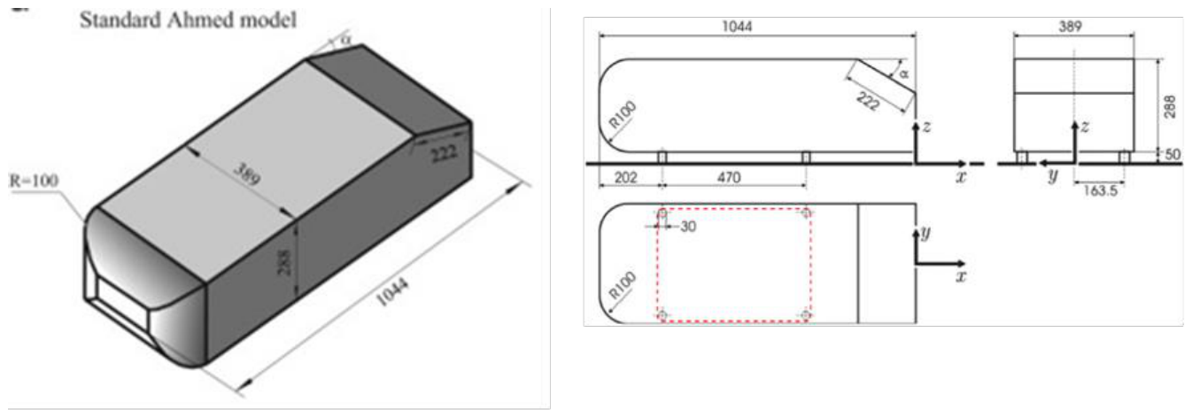
Figure 2.
Computational domain around Ahmed body.
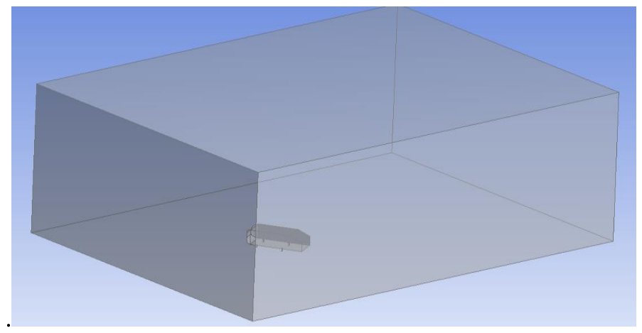
Figure 3.
Drag coefficient of the Ahmed body at various angles of attack.
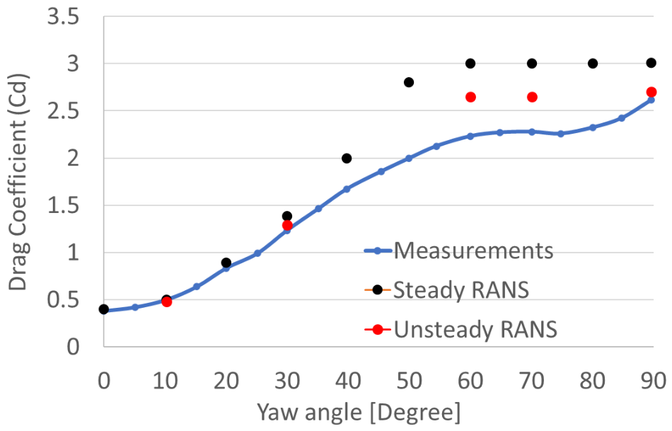
Figure 4.
The CAD geometry received from SevenDOF (left) and The CAD geometry with virtual propeller (right).
Figure 4.
The CAD geometry received from SevenDOF (left) and The CAD geometry with virtual propeller (right).
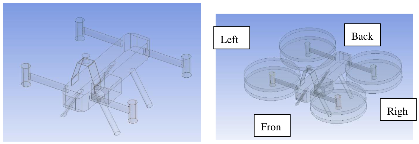
Figure 5.
Geometry in the computational domain (left) and mesh of the computational domain (right)
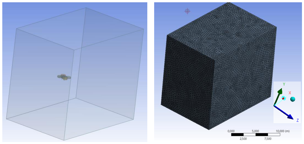
Figure 6.
Pressure contour plot to understand the complexity of the flow.
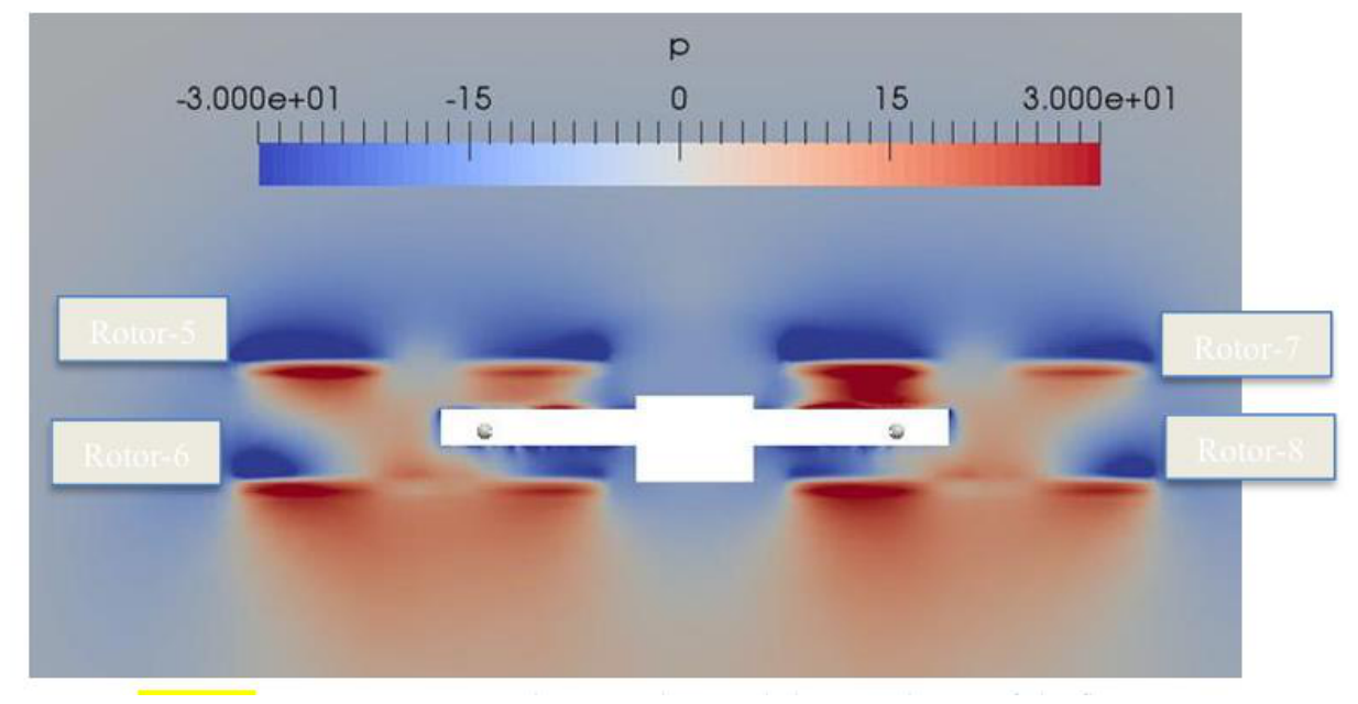
Figure 7.
Drag coefficient, CD(left), and lift coefficient, CL(right), of the V01 configuration as functions of forward velocity at different nose-down angles of attack under stationary-propeller conditions.
Figure 7.
Drag coefficient, CD(left), and lift coefficient, CL(right), of the V01 configuration as functions of forward velocity at different nose-down angles of attack under stationary-propeller conditions.
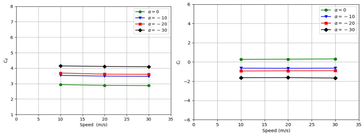
Figure 8.
The pressure distribution on the top and bottom side of the drone when the propeller is not rotating at an angle of attack of 0 degree.
Figure 8.
The pressure distribution on the top and bottom side of the drone when the propeller is not rotating at an angle of attack of 0 degree.
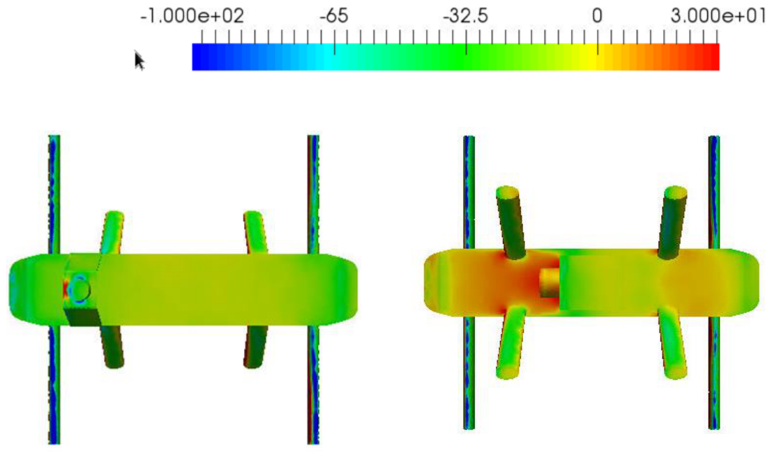
Figure 9.
The pressure distribution on the top side of the drone when the propeller is not rotating at an angle of attack of --10 degrees (nose down).
Figure 9.
The pressure distribution on the top side of the drone when the propeller is not rotating at an angle of attack of --10 degrees (nose down).
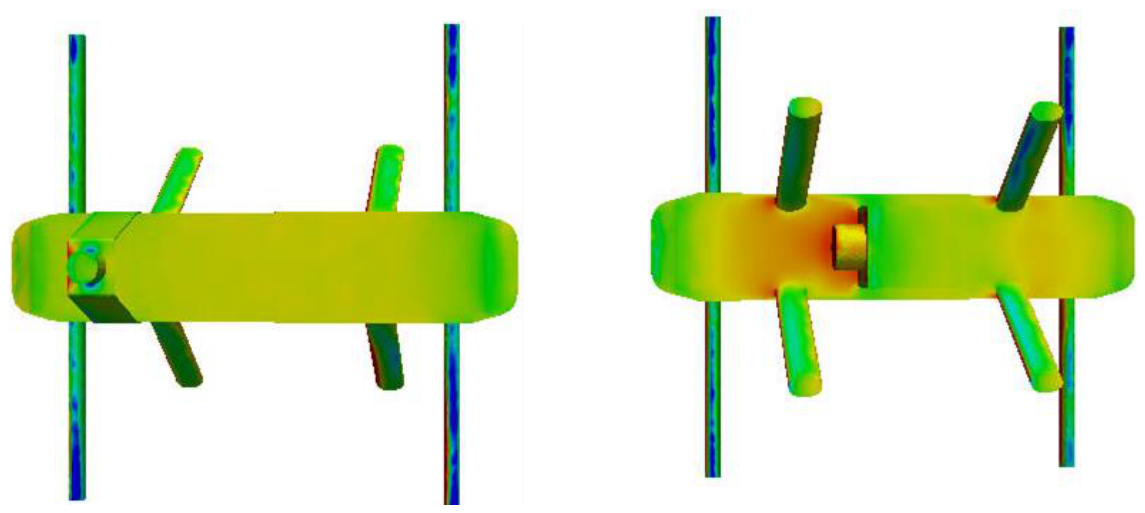
Figure 10.
The pressure distribution on the bottom side of the drone when the propeller is not rotating at an angle of attack of -20 degrees (nose down).
Figure 10.
The pressure distribution on the bottom side of the drone when the propeller is not rotating at an angle of attack of -20 degrees (nose down).
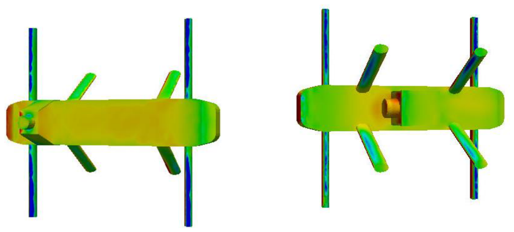
Figure 11.
The drag (Left) and lift (Right) coefficient of V01 with the propeller rotating at 1000 RPM as a function of its speed at various angles of attack (nose down).
Figure 11.
The drag (Left) and lift (Right) coefficient of V01 with the propeller rotating at 1000 RPM as a function of its speed at various angles of attack (nose down).
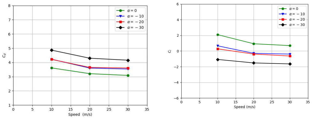
Figure 12.
The drag (Left) and lift (Right) coefficient of V01 with the propeller rotating at 2000 RPM as a function of its speed at various angles of attack (nose down).
Figure 12.
The drag (Left) and lift (Right) coefficient of V01 with the propeller rotating at 2000 RPM as a function of its speed at various angles of attack (nose down).
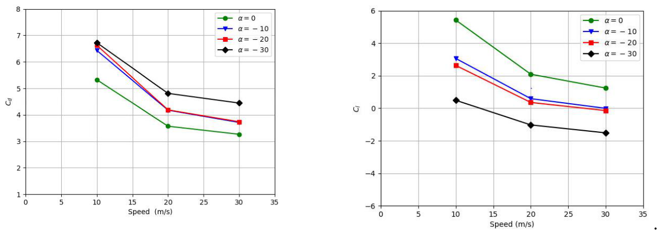
Figure 13.
The drone V02 geometry without (Left) and with virtual propeller (right).
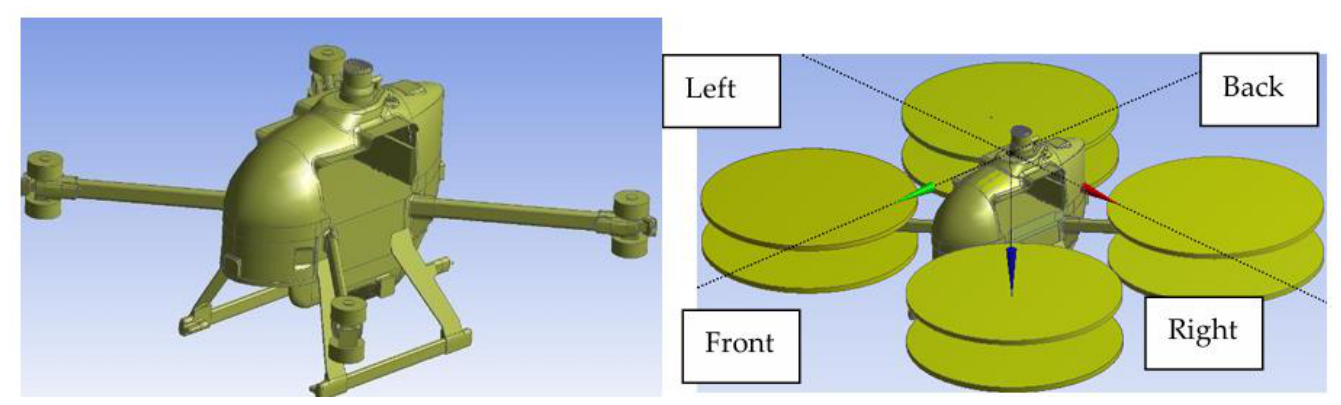
Figure 14.
The drag (Left) and lift (Right) coefficient of V02 without propeller as a function of its speed at various angles of attack (nose down).
Figure 14.
The drag (Left) and lift (Right) coefficient of V02 without propeller as a function of its speed at various angles of attack (nose down).
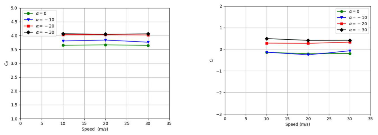
Figure 15.
Surface-pressure distributions over the V01 (left) and V02 (right) configurations at an angle of attack of α = −30∘under stationary-propeller conditions. Both pressure fields are presented using the same scale, ranging from approximately −100to 100Pa.
Figure 15.
Surface-pressure distributions over the V01 (left) and V02 (right) configurations at an angle of attack of α = −30∘under stationary-propeller conditions. Both pressure fields are presented using the same scale, ranging from approximately −100to 100Pa.
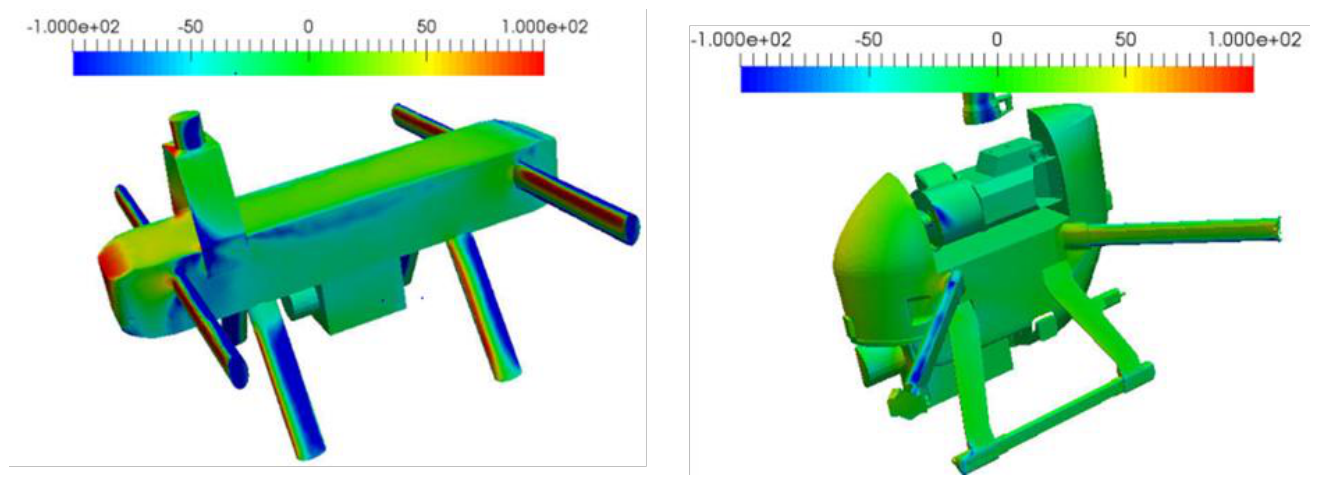
Figure 16.
Drag coefficient, CD(left), and lift coefficient, CL(right), of the V02 configuration as functions of forward velocity at different nose-down angles of attack, with the propellers at 1000 RPM.
Figure 16.
Drag coefficient, CD(left), and lift coefficient, CL(right), of the V02 configuration as functions of forward velocity at different nose-down angles of attack, with the propellers at 1000 RPM.
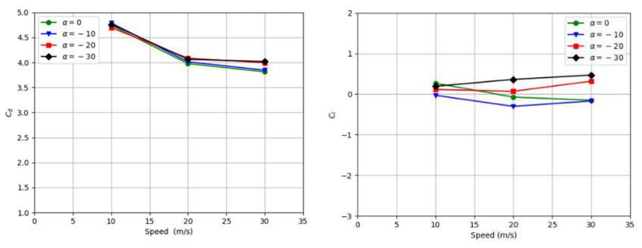
Figure 17.
Drag coefficient, CD(left), and lift coefficient, CL(right), of the V02 configuration as functions of forward velocity at different nose-down angles of attack, with the propellers at 2000 RPM.
Figure 17.
Drag coefficient, CD(left), and lift coefficient, CL(right), of the V02 configuration as functions of forward velocity at different nose-down angles of attack, with the propellers at 2000 RPM.
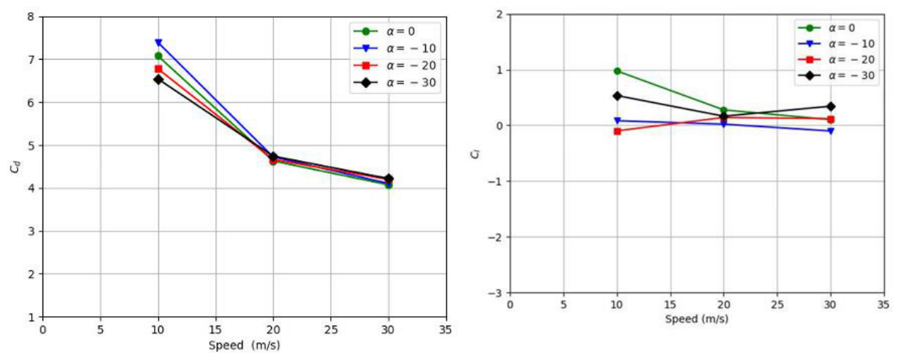
Figure 18.
Comparison of the drag coefficient (left) and lift coefficient (right) of the V01 and V02 configurations at forward velocities of 10 and 30 m/s with the propellers operating at 1000 RPM.
Figure 18.
Comparison of the drag coefficient (left) and lift coefficient (right) of the V01 and V02 configurations at forward velocities of 10 and 30 m/s with the propellers operating at 1000 RPM.
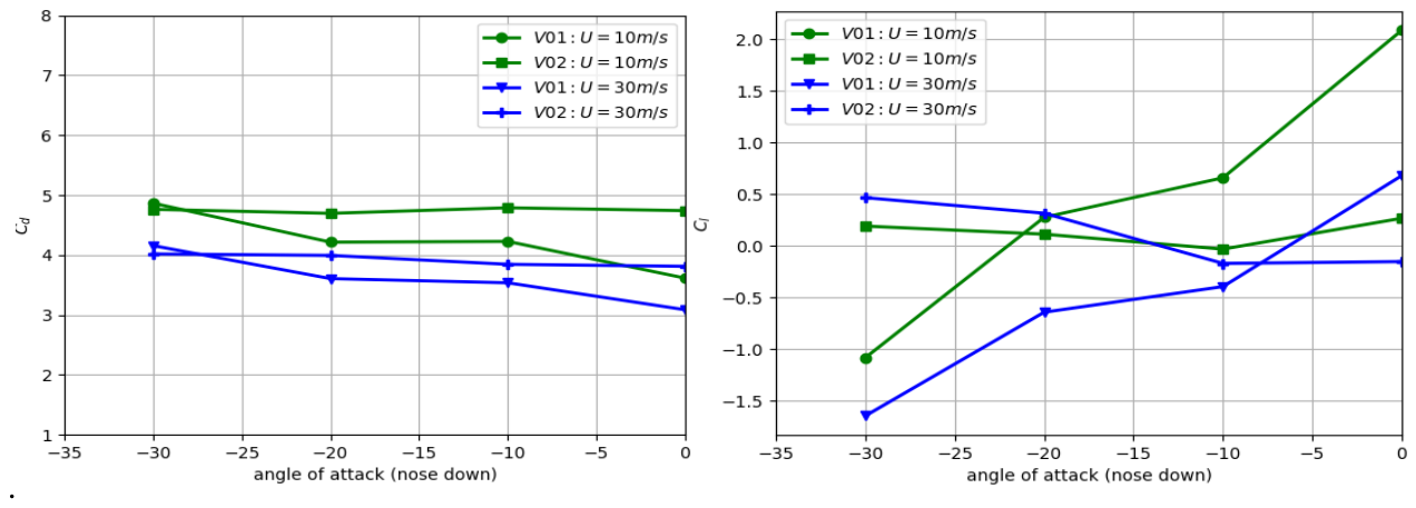
Figure 19.
Comparison of the lift-to-drag ratio of the V01 and V02 configurations as a function of nose-down angle of attack at forward velocities of 10 and 30 m/s with the propellers operating at 1000 RPM.
Figure 19.
Comparison of the lift-to-drag ratio of the V01 and V02 configurations as a function of nose-down angle of attack at forward velocities of 10 and 30 m/s with the propellers operating at 1000 RPM.
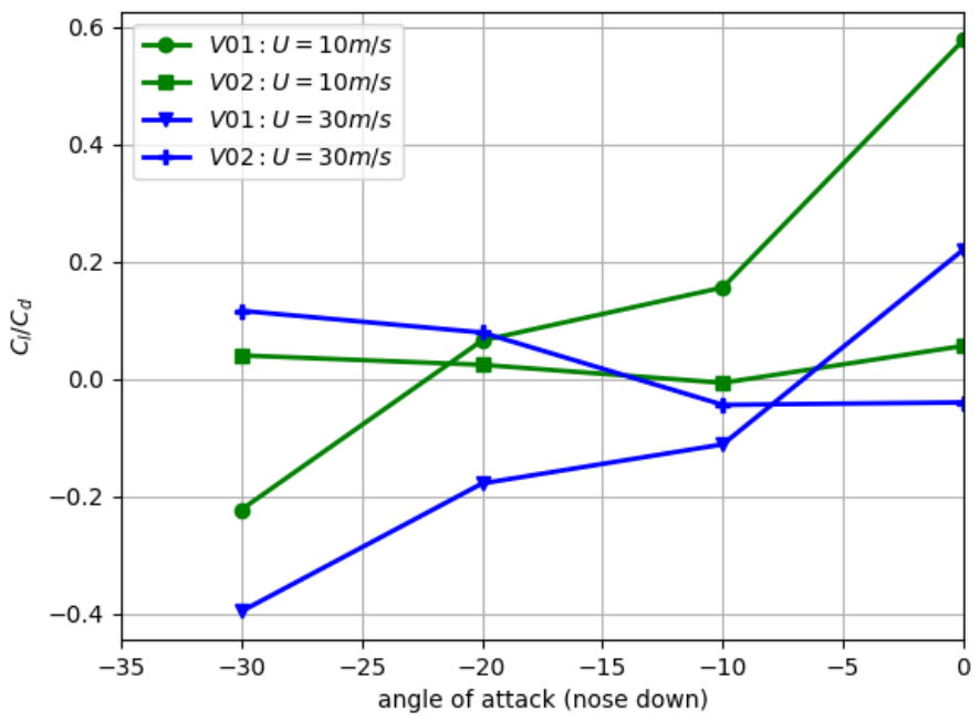

Table 1.
Effect of computational-domain size on the predicted drag coefficient of the UAV at U = 10m/s.
Table 1.
Effect of computational-domain size on the predicted drag coefficient of the UAV at U = 10m/s.
| Domain size | Domain dimensions, L × W × H(m) | CD, RPM = 0 | CD, RPM = 1000 |
|---|---|---|---|
| Large | 28 × 25 × 21 | 3.08 | 3.85 |
| Medium | 24 × 21 × 17 | 2.97 | 3.70 |
| Small | 20 × 17 × 15 | 2.94 | 3.60 |
Table 2.
Effect of mesh resolution on the predicted drag coefficient of the UAV at U = 10m/s.
| Mesh resolution | Number of cells (million) | CD, RPM = 0 | CD, RPM = 1000 |
|---|---|---|---|
| Coarse | 3.20 | 3.10 | 3.70 |
| Medium | 4.80 | 2.97 | 3.60 |
| Fine | 6.44 | 2.94 | 3.50 |
Table 3.
Thrust parameters on the different propellers at 2000 RPM.
| Rotor | Location | Standalone static thrust (N) | Installed thrust (N) | Difference | Relative difference |
|---|---|---|---|---|---|
| Rotor 1 | Left rear, upper | 42 | 36 | −6 | −14.3% |
| Rotor 2 | Left front, upper | 42 | 40 | −2 | −4.8% |
| Rotor 3 | Right rear, upper | 42 | 36 | −6 | −14.3% |
| Rotor 4 | Right front, upper | 42 | 40 | −2 | −4.8% |
| Rotor 5 | Left rear, lower | 25 | 23 | −2 | −8.0% |
| Rotor 6 | Left front, lower | 25 | 31 | +6 | +24.0% |
| Rotor 7 | Right rear, lower | 25 | 24 | −1 | −4.0% |
| Rotor 8 | Right front, lower | 25 | 33 | +8 | +32.0% |
Table 4.
V01 and V02 simulation matrix.
| Propeller rotational speed (RPM) | Angle of attack, α | UAV forward velocity, U(m/s) | Number of simulations |
|---|---|---|---|
| 0 | 0∘, −10∘, −20∘, −30∘ | 10, 20, 30 | 12 |
| 1000 | 0∘, −10∘, −20∘, −30∘ | 10, 20, 30 | 12 |
| 2000 | 0∘, −10∘, −20∘, −30∘ | 10, 20, 30 | 12 |
| Total per UAV configuration | 36 |
Disclaimer/Publisher’s Note: The statements, opinions and data contained in all publications are solely those of the individual author(s) and contributor(s) and not of MDPI and/or the editor(s). MDPI and/or the editor(s) disclaim responsibility for any injury to people or property resulting from any ideas, methods, instructions or products referred to in the content. |
© 2026 by the authors. Licensee MDPI, Basel, Switzerland. This article is an open access article distributed under the terms and conditions of the Creative Commons Attribution (CC BY) license (http://creativecommons.org/licenses/by/4.0/).
Copyright: This open access article is published under a Creative Commons CC BY 4.0 license, which permit the free download, distribution, and reuse, provided that the author and preprint are cited in any reuse.