

Submitted:
13 October 2026
Posted:
14 October 2026
You are already at the latest version
Abstract
This paper examines the undesirable yet inevitable influence of loading system compliance on specimen deformation measurements during testing—a problem that has become typical and remains consistently relevant in the field of mechanical materials testing. Of the two possible approaches to addressing this issue—increasing the stiffness of the loading system or applying corrections to the measurement results—this work focuses primarily on the latter. A mathematical model describing the interaction between loading system components was developed using mixed additive-multiplicative scaling, and a cost-effective method for neutralizing the effect of loading system compliance was proposed. It is demonstrated that applying this method is theoretically equivalent to conducting tests on a virtual machine with infinite loading system stiffness. The method utilizes load-displacement data obtained from two compression tests performed under identical conditions: one with the specimen and one without it. The method was validated using aluminum specimens by comparing the calculated elastic modulus (75.6 GPa) with the established reference range (72–75 GPa). Additionally, the method was used to determine the elastic modulus of amphibolite and to generate corrected load-displacement diagrams. A comparative analysis revealed a source of error inherent in the traditional compliance summation method. Overall, the proposed approach, model, and method—based on additive-multiplicative correction of compression test results—offer a structured and interpretable supplement to traditional techniques, opening new avenues for enhancing the accuracy of both direct and indirect measurements of material properties.
Keywords:
materials testing
; machine stiffness
; modulus of elasticity
; amphibolite
1. Introduction
This article examines the influence of the stiffness (the reciprocal of compliance) of a testing machine’s loading system on the results of material compression tests. This undesirable yet unavoidable influence of the loading system’s stiffness on specimen deformation measurements is a typical issue in mechanical testing. The inevitability of this effect stems from the fact that infinitely stiff materials do not exist in nature. Consequently, the testing machine’s displacement sensor (unless the digital image correlation (DIC) method [1] is used) records the total deformation, which consists of two components: the specimen’s intrinsic deformation and a hidden component caused by the deformation of the loading system’s elements. The hidden component distorts the measurement results; therefore, its influence must be minimized as far as possible, given the continuously growing requirements for the accuracy and cost efficiency of both direct and indirect measurements of material properties. In response to these demands, between 1935 and 1971, engineers developed and began to implement stiff testing machines equipped with feedback control systems [2]. Research in this area of applied studies remains ongoing today [3,4,5].
Increasing the stiffness of the loading system is a reliable means of improving the accuracy of measured specimen deformations during material testing. However, the technical possibilities for enhancing the stiffness of loading systems are constrained by the physical and mechanical properties of the actual materials from which the system components are manufactured. Therefore, it becomes increasingly relevant to develop methods that do not aim to increase the real stiffness of the loading system, but rather to mathematically model the physical interaction between the main elements of the machine–specimen system in order to correct the measurement results at the data processing stage [5,6].
Such correction complements the capabilities of DIC technologies and, in the case of testing non-standard small-sized specimens, may represent the only feasible method [5]. Nevertheless, it should be noted that correction methods rely on test results previously obtained using a specific testing machine. Thus, correction techniques serve as an additional tool in the suite of methods available for precise investigations of material properties.
The method most widely cited in the literature for correcting indirect measurements of specimen stiffness is based on the principle of determining the stiffness of the loading system and subtracting it from the raw data obtained for the “machine–specimen” system [7,8]. However, recent studies [5,6,9] have demonstrated that this approach is not straightforward to implement. By presenting new findings in this field, these studies highlight the relevance of the issue and identify potential avenues for future development. Despite a number of significant results, the development of a sufficiently universal and accurate correction method for precisely determining the elastic modulus and the load–displacement relationship remains a pressing challenge [2,7,10,11,12,13], and certain aspects remain a subject of debate [14], underscoring the overall importance of the problem.
It should be noted that high-stiffness testing machines are expensive; however, they are essential for applied research, meaning that the high cost inherent in such unique setups does not constitute a critical barrier to progress in this field. At the same time, laboratories continue to use relatively low-stiffness machines, which can be quite effective for solving many engineering problems if measurement correction algorithms are integrated into their software [5]. Implementing correction algorithms in conjunction with a testing machine of any stiffness potentially enhances the accuracy of experimental data on materials and expands the machines’ capabilities without increasing the cost of mechanical components.
Thus, improving methods and algorithms for correcting measurement results during or after specimen testing is a pressing issue, and solutions to this problem are in demand across a wide range of applications involving the study of rock, concrete, frozen soil, wood, and other materials [15,16,17,18,19].
A review of the literature shows that, despite significant progress in this field, certain gaps remain in the mathematical modeling of the physical interaction between the components of the “testing machine–specimen” system. For example, to the best of our knowledge, the issue of neutralizing the effect of loading system stiffness during compression tests using additive-multiplicative correction—a method proposed in the present study—has not been addressed previously, although the technical effectiveness and economic viability of the additive-multiplicative approach have already been demonstrated in other fields of applied research [20].
The primary objective of this study is to develop a effective method for determining the intrinsic stiffness and elastic modulus of a specimen, as well as the corrected load-displacement curve under uniaxial compression in a conventional testing machine, by eliminating the influence of the loading system’s and specimen’s compliance. The loading system of the testing machine is assumed to be configured as a series arrangement of elements.
Unlike previously published works, this study employs a mixed additive-multiplicative approach to develop a new, interpretable mathematical model describing the influence of the loading system stiffness and the specimen itself on measurement results. The model was verified by comparing calculated data with known values of the elastic modulus for aluminum [21]; this material was selected because its properties exhibit significantly less variability than those of rock, while its elastic modulus values are comparable to those of certain granites and similar materials [15,17]. Load-displacement curves obtained from two compression tests—one with a specimen and one without—served as the input data for the calculations. New relationships were derived to determine the corrected stiffness coefficient and the elastic modulus in compression. A method for constructing a corrected load-displacement diagram is proposed. A calculation example using amphibolite specimens is presented, yielding realistic elastic modulus values consistent with geotechnical research data.
This paper proposes an additive-multiplicative method that makes it possible to neutralize the effect of the loading system’s compliance on the load-displacement relationship and to indirectly determine stiffness and the modulus of elasticity (which is related to stiffness by a linear dependency described by Hooke’s law). The use of the additive-multiplicative approach accounts for the nonlinearity of load-displacement curves and ensures high data accuracy; it also simplifies the correction procedure compared to other methods, thereby contributing to the scientific substantiation of experimental techniques for determining material properties in applied research.
2. Stiffness Coefficients Correction
2.1. Preliminary Stiffness Coefficient Values
This section addresses the determination of the stiffness parameters of the loading system and the specimen, as well as the elastic modulus of the specimen material, prior to the application of the relevant corrections. This is because stiffness coefficients and the elastic modulus—unlike displacement and load—are determined indirectly by substituting measured displacement and load values into the corresponding formulas, rather than through direct measurement.
The stiffness of a testing machine’s loading system refers to the ability of its structure (load frame, platens, and auxiliary devices) to resist deformation under load.
The primary output of the tests consists of load (P) and displacement (u) values measured at intervals—for example, every 0.01 s. These data are visualized using a load-displacement diagram. Stiffness K is determined based on the load increment ΔP and displacement increment Δu [8].
Using local linearization of the load-displacement curve and a central finite-difference approximation in the vicinity of point i, one can write: [22]. This numerical differentiation process is sensitive to noise. To smooth the K(u) curve, an alternative version of the same formula can be used:
, i = m + 1,…,n − m.
The value m = 1 corresponds to the K(u) curve without smoothing. A comparison of the variants with m equal to 50, 250, and 500 is provided in Appendix A.
The characteristic K (2) plays a dual role: from a physical perspective, it is the stiffness coefficient, and from a geometric perspective, it is the slope coefficient, which determines the angle of inclination of the tangent to the curve representing the relationship between load and displacement, passing through the point with coordinates (ui, Pi).
Using Equation (2) and the measurement results, it is possible to calculate the stiffness of the specimen at any point on the curve with the measured values of load and displacement. However, when it comes to the material’s elastic modulus, it is generally accepted that the standard value of stiffness and elastic modulus corresponds to the point at which the specimen’s stiffness and the linearly related elastic modulus are at their maximum: . The elastic modulus and stiffness of a specimen with length L and cross-sectional area A under uniaxial loading are related by the equation . If the stiffness of the specimen (2) is determined, the elastic modulus can be calculated: .
Testing machines may employ additional devices to transfer the load to the specimen, such as platens of various sizes, grips, and a leveling device in the form of a spherical seat. Using a spherical seat to transfer the load to the upper bearing platen allows for the compensation of slight misalignments in the specimen’s bearing surfaces. According to the ASTM E9-19 standard, the use of a leveling device permits a relaxation of strict parallelism requirements for the bearing surfaces, as the device (ball joint) compensates for minor, random deviations from the specimen’s ideal geometry. However, as this additional device is part of the load-transfer assembly, it reduces the overall stiffness of the mechanical system compared to a configuration without it—a factor that, in turn, affects the accuracy of the test results. This does not imply that the use of a leveling device should be abandoned; on the contrary, it is essential, provided that the influence of its compliance on the measurement of the specimen’s intrinsic stiffness is neutralized.
The following terms and indices are used below to designate the components of the mechanical system under consideration: 1—testing machine loading system; 2—ball joint; 3—test specimen (Figure 1). To avoid overly cumbersome terminology, components 1, 2, and 3 are referred to below as the “machine,” “ball joint” and “specimen,” respectively. For example, the stiffness of the “machine–ball joint–specimen” system is denoted as K123.
The stiffness of a specimen or other mechanical system is determined not directly, but indirectly, through a mathematical relationship with quantities for which direct measurement methods exist. Indirect measurement of the stiffness coefficient of a specimen means determining this coefficient by substituting the measured values of load and displacement into the appropriate formula, for example, into the formula (2).
If the “machine–ball joint–specimen” mechanical system consists of N elements connected in series, then the same force acts on each element. The stiffness of such a system is defined as [2]. In the case under consideration, . This equation shows that the stiffness of the specimen (K₃) affects the stiffness of the “machine–ball joint–specimen” system. However, the stiffness of the system (K₁₂₃) also affects the stiffness of the specimen: ; .
Since the specimen stiffness—determined by the aforementioned ratio EA/L—influences the stiffness of the entire system (and, consequently, the measured displacements), testing specimens made of the same material (with an identical modulus of elasticity) but having different A/L ratios (and, thus, different stiffnesses) yields varying stress and strain values; this phenomenon has been investigated in a number of studies [6,17,23]. Ideally, material properties should be independent of the A/L ratio. In practice, however, testing conditions are far from ideal [5,9]; therefore, specimen shape and size affect the entire force-displacement curve, a fact demonstrated in both classic [2] and recent studies [3,4,14]. These factors underscore the importance of the aforementioned development of a method to neutralize the influence of specimen stiffness and other non-ideal testing conditions in real testing machines.
When developing a stiffness correction method, it is necessary to include a procedure for assessing the accuracy of the final result. The value of the elastic modulus is not known beforehand and must be determined experimentally. The accuracy of the stiffness coefficient and elastic modulus values obtained through indirect measurements (after applying the correction) can be assessed by comparing them with published data. If such a comparison confirms sufficiently high accuracy and the methodology itself is physically sound, the method can be applied to experimentally determine the elastic modulus of other materials with unknown elastic moduli—such as rocks, which are characterized by significant variability in their elastic modulus and other physical properties [17,24,25]. Regarding the choice of aluminum specimens to verify the method’s effectiveness, it should be noted that this choice ensures a sufficiently reliable assessment. The elastic modulus of the specimen material (D16T aluminum alloy) falls within a relatively narrow range (72–75 GPa), making it unlikely that an obtained value would fall within this interval by chance—unlike rocks, which exhibit great variability in mechanical properties.
By way of illustration, the results of compression tests on an aluminum specimen (23.6 mm in diameter and 51 mm in height) performed at a constant deformation rate of 0.2 mm/min are presented below. Figure 2 (a continuation of Figure 1) shows the load-displacement relationship for the “machine–ball joint–specimen” system (green curve 123). Loading of the machine at the same rate was also carried out without the specimen (red curve 12). Load and crosshead displacement values were recorded at 0.01 s intervals.
From a geometric standpoint, the stiffness coefficient K123 is determined by the slope of the tangent line passing through the point with coordinates u123, P123 (Figure 2). The equation of the tangent line is
P123 =a123 + K123u
From Equation (3), the displacement u123—which will be needed in the subsequent discussion—can be expressed:
u123 =b123 + C123P
In terms of physical meaning, the quantity represents the compliance of the “machine–ball joint–specimen” system; .
Figure 2 shows that the stiffness of the “machine–ball-and-socket joint–specimen” system increases from zero to a value of (2) and then decreases. The point of maximum stiffness lies within a region that can be approximated by a straight-line segment. From a physical standpoint, this corresponds to the linear-elastic deformation stage of the material; a similar stage is observed during the uniaxial compression of rocks and similar materials [11,15].
2.2. Stiffness of the “Machine–Ball Joint” System (Without Specimen)
The load-displacement curve for compression without a specimen is shown in Figure 2 (red curve). Loading the testing machine without a specimen is equivalent to self-testing the loading system (including the spherical seat) or testing a specimen with infinite stiffness [25]. This curve reflects two stages of the loading process: a non-linear initial stage and a linear subsequent stage. The non-linearity of the first stage can be attributed to the closing of clearances and the gradual adaptation of the contacting surfaces to the increasing load during the testing process.
The linear stage emerges after the contact interaction between the elements of the mechanical system has stabilized. The transition point from the nonlinear stage to the linear stage can be determined by equating the first derivatives at points i and i + 1 using formula (2). This makes it possible to determine the stiffness of the “machine–ball joint” system (K12), as well as the slope and equation of the linear segment that models the linear stage of the system’s operation
P12 = a12 + K12u.
Using Equation (5), one can determine the dependence of the displacement u12 on the load P, which is required for the subsequent discussion:
u12 = b12 + C12P.
In a physical sense, the quantity represents the compliance of the “machine–ball joint” system.
2.3. Uncorrected Stiffness of the Test Specimen
As noted above, the specimens have a specific geometric shape and dimensions. Let A be the cross-sectional area and L the height (length) of the specimen; let ΔL be the deformation of the specimen under the load P, determined from measured displacements. Applying Hooke’s law, we can write: , , , , . Referring to Figure 2, we can write ΔL = u3 = u123 − u12; the specimen stiffness K3 is defined as
Formula (7) determines the stiffness coefficient of the specimen prior to correction. If necessary, the stiffness coefficients of the “machine–ball assembly” and “machine–ball joint–specimen” systems may be reduced:
2.4. Adjustment of Stiffness Coefficients
2.4.1. Working Hypothesis and Main Result of the Study
Based on the preceding preliminary analysis of the physical and geometric aspects of the “machine–ball joint–specimen” mechanical system’s operation, it can be shown that neutralizing the effect of the loading system’s stiffness is possible using additive corrections. However, the correction terms themselves must include scaling factors for the values being adjusted—that is, an additive-multiplicative correction must be employed. The corrected specimen stiffness value can then be expressed as follows (definitions of the subscripts are provided below):
Regarding Equation (11), the problem lies in developing a method to determine the corrections using the measured displacements u12 and u123 (Figure 2). Let us consider the solution to the problem in a general form.
If a mechanical system consists of n elements, a decomposition approach allows it to be viewed as a system comprising two parts: one containing (n − 1) elements and the other a single element. The part of the system consisting of multiple elements can be treated as a single unit (or super-element). For instance, in the case discussed above, one part of the mechanical system is a discrete element (the specimen), while the other consists of two elements (the testing machine’s loading device and a ball joint) (Figure 2). This example demonstrates that by treating the specimen as one element and grouping the remaining elements into another (a super-element), one can perform the necessary analysis of multi-element mechanical systems in testing machines. Hence, to substantiate the proposed approach for the additive-multiplicative adjustment of stiffness coefficients, it suffices to consider a two-element system.
Consider a system consisting of two elements, i and j, with stiffness coefficients Ki and Kj, respectively. Based on the preceding analysis of the physical and geometric aspects of the problem, the working hypothesis of this study can be formulated as follows:
the additive-multiplicative correction AddMulti,j to the stiffness coefficient Ki— reflecting the influence of element j— is proportional to the stiffness coefficient Ki and the deformation of element j, but inversely proportional to the sum of the deformations of elements i and j, as determined by the displacements ui and uj:
In physical terms, the quantity defined by the ratio represents the stiffness per unit of total deformation (defined as the sum ui + uj); thus, formula (11) characterizes the influence of the deformation uj. The ratio acts as a multiplier that scales the additive correction resulting from the influence of element j.
The overall stiffness of the loading system changes when a specimen is added to the system. As noted above, these changes depend on the stiffness of the specimen. Therefore, it should be noted that in the system under consideration—comprising two elements, i and j, with stiffness coefficients Ki and Kj—the additive-multiplicative correction AddMulti,i for the stiffness coefficient Ki (resulting from the influence of element i) is proportional to the stiffness coefficient Ki and the deformation of element i, but inversely proportional to the sum of the displacements of elements i and j:
When making corrections, it is necessary to take into account the influence of all elements of the mechanical system, as shown in Equation (10). Then
Equations (11) and (13) formally express the working hypothesis and the main result of this study, the details of which are discussed below.
To elaborate, it should be noted that in the case under consideration (Figure 2), when determining the corrected specimen stiffness using formula (13) for the load P = P123, the following data are used: Ki = K3, , uj = u12. Thus, Regarding K3, see Equation (7).
If it is necessary to determine the corrected stiffness of the “machine–ball joint” system, then Ki = K123, ui = u12 , . Regarding $K12, see Equation (8).
To adjust the stiffness of the “machine–ball joint–specimen” system, the following data are used: Ki = K123, the system deformation is ui = u123 = u12 + u3, uj = 0. . Regarding K123, see Equation (9).
As noted above, the working hypothesis comprises two aspects—additive and multiplicative—which can be examined using the example of a specimen whose deformation is represented in Figure 2 as u3 = u123 − u12. Accordingly, the mathematical expression of the working hypothesis can be presented in two equivalent forms representing the same quantity but from two different perspectives, reflecting multiplicative and additive correction.
Comparing lines (14) and (13) makes it possible to write the formulas for calculating the correction terms in the following form:
In physical terms, the fraction in expression (15) represents the portion of the total correction accounted for when adjusting the specimen stiffness. This means that the effect of specimen compliance is taken into account, while the effect of the remainder of the total correction is not. The fraction corresponding to the remainder of the total correction is determined by the ratio in Equation (16). The sum of the fractions equals 1 (full correction):
2.4.2. Multiplier Effect
Equation (14) shows that multiplicative correction (scaling) consists of multiplying the value K3 by a correction factor (multiplier):
This coefficient increases or decreases the final value proportionally, depending on the parameters u123 and u12.. Given the physical context of the problem, u123 > u12; therefore, the adjusted value is greater than the initial one.
If u123 ≫ u12, then and .
For infinitely stiff testing machines,u12 = 0; in this case, and and .
The term “1” in formula (18) ensures that if the difference (u123 − u12) approaches zero, then and the corrected value remains unchanged(). This implies that the correction to the test results for an infinitely stiff machine is zero. However, infinitely stiff systems do not exist; therefore, correcting the measurement results is necessary.
If the specimen stiffness is infinitely high, then u3 = u123 − u12 = 0, , and .
2.4.3. Additive Correction
The additive adjustment (application of a correction) shown in (14) consists of adding a correction to the initial value of K3: K3 + ∆K3. Here
A distinctive feature of this additive term is its dynamic nature. It is not constant (like a classical zero shift) but depends on the quantity being corrected (K3) and on changes in the parameters u123 and u12; this additive term models the nonlinearity of the loading process.
Theoretically, if the machine stiffness is infinitely high, then u12 = 0; in this case, ∆K3 = K3, and If u123 ≫ u12, then ∆K3 → K3 and .
If the specimen possesses infinite stiffness, then u3 = u123 − u12 = 0, ∆K3 = 0 and .
By analogy with $, we can write:
In a physical sense, the fraction in Equation (20) represents the proportion of the total correction accounted for when adjusting the specimen stiffness. This implies that the effect of specimen compliance is taken into account, while the effect of the remainder of the total correction is not. In this case, the proportion corresponding to the remainder of the total correction is defined by the fraction in Equation (19). The sum of the proportions equals 1.
Sum of the stiffness coefficients of the specimens and the “machine–ball joint” system, in accordance with Equation (10), leads to the following relationship:
The stiffness K3 can be determined using formula (7). Thus, taking into account formulas (7) and (13), we obtain the same result in general form:
2.4.4. Determination of the Corrected Modulus of Elasticity Value
The corrected stiffness coefficient (22) is used to calculate the corrected elastic modulus of the specimen material, which has a cross-sectional area A and a height (length) L. Using Hooke’s law, as shown in the first part of Section 2.3, one can write:
Thus, modeling the uniaxial compression testing process described by equations (1)–(23) led to a simple method for eliminating the influence of the compliance of all loaded elements on the results of measuring specimen stiffness and material elastic modulus.
2.5. Comparison with the Generally Accepted Method and the Need for Its Improvement
The conventional method for determining the stiffness of a testing machine’s loading system is based on a mechanical model consisting of springs connected in series [2,8]. Using this model, the following equations can be written:
The stiffness coefficient K3 can be determined in two ways: (I) as specified in (24), and (II) using Equation (7) after transforming it by taking into account equations (4) and (6), as shown below in (25).
A comparison of expressions (24) and (25) reveals that the widely used equation of the form (24) for determining stiffness K3 lacks the term . Geometrically, the quantitiesb123 and b12 represent the abscissae of the points where the tangents to curves 12 and 123 intersect the horizontal coordinate axis (Figure 2). Since actual load-deformation relationships are nonlinear during the initial loading stage, b123 ≠ 0 and b12 ≠ 0. Consequently, equations (24) are not exact in the general case.
It should be noted that the springs in model (24) are linear-elastic elements [2,8] for which the tangent and secant stiffness coincide, whereas the specimens and the loading systems of the testing machines undergo nonlinear deformation during the initial stage of loading. This nonlinearity arises from an increase in system stiffness due to the gradual closure of cracks in the specimen and the elimination of initial clearances in the loading system.
However, the augmented stiffness coefficient K3 in line (25) is not final, as shown by equations (13) and (22).
It should be noted that the transformations (25) are presented here solely to clarify the proposed method for neutralizing the effect of the testing machine’s loading system compliance. These transformations are not required for the practical application of the proposed method, as the specimen stiffness coefficient K3 is determined prior to applying the correction using only three measured quantities via formula (7). To adjust the value of K3, the formula (13), derived in this study, is used.
2.6. Workflow
1. Conduct the tests and plot the load–displacement diagram (Figure 2). On the obtained curve, identify the point where the tangent stiffness reaches its maximum. This can be determined, for example, using Equation (2): . For this point, determine the load P123 and and the corresponding displacement u123.
2. In the same loading mode, run the testing machine without a specimen and plot the load–displacement curve (Figure 2). On this curve, identify the point corresponding to the load P123 specified in Step 1, and determine the displacement u12 for this load.
Note. If the tests are performed under a constant crosshead displacement rate (e.g., 0.2 mm/min), then condition P123 = P12 does not hold. In this case, transform the u12 vector so that its i-th element equals the crosshead displacement in the no-specimen test at the load corresponding to the i-th element of the P123 vector. This transformation can be carried out using interpolation, approximation [25], or other methods [26]. However, if tests both with and without the specimen are conducted at the same loading rate (e.g., 700 N/s), such a transformation is not required, since in this case the i-th element of P₁₂₃ is equal to the i-th element of P₁2—that is, the condition P₁₂₃ = P₁₂ is satisfied automatically (Figure 2).
3. Determine the uncorrected specimen stiffness coefficient using Equation (7).
4. Calculate the corrected specimen stiffness coefficient using Equation (22).
5. Compute the corrected value of the material’s elastic modulus for the specimen with cross-sectional area A and height (length) L using Equation (23).
3. Results
3.1. Testing of Aluminum Specimens
To validate the model proposed in Section 2, mechanical tests were carried out on cylindrical specimens with dimensions D=23.6 mm and L = 51mm (Figure 1, green curve). The specimens were fabricated from the D16T aluminum alloy. The tests were performed under a constant strain rate of 0.2 mm/min. Under the same loading conditions, the testing machine was also operated without a specimen, yielding the reference response (Figure 1, red curve).
The primary objective of this experimental stage was not to characterize the material properties of the specimens—the elastic modulus of the alloy is known a priori—but to assess whether the proposed approach and the stiffness correction method, based on Equations (7), (22), and (23), can fully account for the loading system’s stiffness. The aim was to obtain a sufficiently accurate estimate of the elastic modulus using a conventional testing machine.
Aluminum specimens were selected for model validation because the elastic modulus values for aluminum and its alloys have been reliably established in numerous studies, exhibiting relatively low variability: 70–76 GPa [21,27]; 72–75 GPa [28].
Figure 3 presents the load–displacement curves before and after the correction procedure.
Table 1 presents the initial data and the results of calculating the corrected stiffness coefficient and the modulus of elasticity for the aluminum specimen using equations (7), (22), and (23).
The obtained value of the elastic modulus (75.6 GPa) lies at the upper limit of the aforementioned range of values (70–76 GPa) reported in the literature [21,27]; 72–75 [28]. The extent to which the upper limit for the material under investigation (75 GPa [28]) is exceeded amounts to . From a physical standpoint, this is entirely expected, as even ultra-stiff loading systems do not possess infinite stiffness; due to their inevitable—albeit minimal—compliance, measured displacement values are slightly overestimated, whereas the specimen’s stiffness coefficient and elastic modulus are slightly underestimated. Consequently, completely eliminating the influence of the loading system’s compliance (or stiffness) on displacement measurement results makes it possible to obtain estimates of stiffness and elastic modulus that correspond to the upper limit. The method described above, formalized by equations (1)–(25), models precisely this scenario of completely eliminating the unwanted influence in question.
It should be noted that, as mentioned above, the ball joint allows the load on the specimen to be centered (Figure 1); however, it reduces the overall stiffness of the loading system compared to its rated specifications, as it acts as one of the elements connected in series within the loading system. Using Equations (8) and (13) and the data from Table 1, the stiffness of the “machine–ball joint” system under load P_123 can be determined: P123: . In this case, the specimen stiffness is , that is, the stiffness of the testing machine is 2.6 times lower than that of the specimen, which, according to established terminology [2], corresponds to a “soft testing machine.” Nevertheless, the influence of the loading system stiffness—including the stiffness of the additional device—is neutralized by using the proposed method for correcting measurement results, as evidenced by the sufficiently accurate determination of the elastic modulus (Table 1).
3.2. Method Limitations
It should be noted that in the experiment under consideration, the elastic modulus of the specimen material (aluminum) is approximately one-third that of the support plates (steel). Consequently, local deformations of the support plates in the contact zone are negligible. However, testing stiffer specimens with reduced cross-sectional dimensions increases local deformation of the support plates at the contact interface, thereby increasing their contribution to the recorded specimen displacements (strains). In such cases, it is advisable to use high-stiffness support plates made of a material with a higher elastic modulus. Thus, the method proposed in this paper is subject to a limitation regarding support plate stiffness.
An alternative approach to analyzing errors in recording stress-strain curves during compression tests without an extensometer, as well as a correction method for non-standard, reduced-size specimens, is proposed in [5].
Another limitation on the applicability of the developed method—which corrects for the influence of loading-system compliance on measured displacements—relates to the accumulation and explosive release of elastic strain energy within the “machine–ball joint–specimen” system during the post-peak deformation stage (specifically when the specimen material is brittle, such as rock, rather than ductile aluminum). Figure 3 shows that the specimen’s strain energy during the pre-peak stage—defined as the area under the load-displacement curve—accounts for approximately 28% of the total strain energy of the “machine–ball joint–specimen” system; this serves as a nominal efficiency coefficient for the testing machine. In an infinitely stiff loading system, displacements during testing without a specimen would be zero, the load-displacement curves for the specimen and the “machine–ball joint–specimen” system would coincide, and the input energy would be consumed solely by specimen deformation. Consequently, it is advisable to develop and utilize testing machines with the highest technically feasible loading-system stiffness; the issues arising in this context and methods for addressing them are discussed in [3,4].
Nevertheless, based on the description provided above and the analysis of the interaction between the testing machine components, it can be asserted that a material testing model for a virtual machine with infinite stiffness has been developed; this model is theoretically grounded and yields physically consistent results. The developed approach, model, and method relax the stiffness requirements for the loading systems of testing machines; furthermore, the method is suitable for refining indirect measurements of the elastic modulus and for correcting load-displacement diagrams.
The application of this method to the testing of amphibolite is discussed in the next section.
3.3. Amphibolite Testing
Table 2 presents the initial, intermediate, and derived data for determining the stiffness coefficient and modulus of elasticity of amphibolite (Figure 4) using the presented measurement result correction method.
When discussing the data presented in Table 2, it should be noted that the literature contains limited information on the mechanical properties of amphibolites from this region. Study [29] reports measured elastic modulus values for amphibolites from the Karelian (107–110 GPa) and Kola-Belomorian (53–72 GPa) complexes. For the amphibolites investigated in the present study (Table 2), the elastic modulus is lower, ranging from 19 to 39 GPa. This reduction in the elastic modulus—along with its significant variability (24%)—may be attributed to specific formation conditions, the influence of spatially heterogeneous multi-stage deformation, and compositional heterogeneity of the Earth’s crust in the region. This explanation is consistent with the differences in elastic modulus values observed for the aforementioned amphibolites of the Karelian and Kola-Belomorian complexes. When discussing the possible causes of rock deformation and subsequent fracturing [30], it is also necessary to consider the impact of earthquakes that occurred in the region 9,000–11,000 years ago and local seismic deformations [31,32] within the context of preceding geodynamic processes [32,33].
However, the available data are insufficient to draw definitive conclusions regarding the reduced elastic modulus, as gaps remain in this field of research; various methods are being employed to address them, including the measurement of the physicomechanical properties of amphibolites [28,29,34,35]. The method for the precise measurement of the elastic modulus developed in this study will provide additional information; When combined with the recording of sampling locations and the use of other methods, this information can help improve the efficiency of exploration activities and refine assessments of mineral resource quality.
4. Discussion
To the best of our knowledge, no previous study has employed an additive-multiplicative measurement correction during compression testing to determine specimen stiffness and material elastic modulus, or to construct load-displacement curves. Thus, the primary contribution of this study lies not only in simplifying the acquisition of accurate data regarding specimen stiffness, elastic modulus, and load-displacement behavior, but also in extending the capabilities of conventional testing machines for material property analysis. Since infinitely stiff materials do not exist in nature, there are inherent limits to improving measurement accuracy by simply reducing the compliance of the testing machine’s loading system; the proposed method for neutralizing the effect of loading-system compliance overcomes this limitation. This method is suitable for use with testing machines of any stiffness.
It should be noted that this study examines the specimen’s behavior only during the pre-peak stage of the test. The post-peak stage requires a separate analysis, taking into account existing studies [3,4,14].
Other aspects open to discussion are addressed in the concluding parts of Section 3.2 and Section 3.3. It should be noted, however, that despite the good consistency of the test results for aluminum specimens (Section 3.1) and the geotechnical interpretable experimental data for amphibolite (Section 3.3), the volume of experimental data obtained using the proposed method is clearly limited. Therefore, future research will involve testing the method on other rock types and systematizing the resulting data.
5. Conclusions
Based on the research and development of a low-cost method to neutralize the effect of the compliance of all load-transmitting elements during compression testing, the following conclusions can be drawn.
The mechanisms of mutual influence between the elements of a testing machine’s loading system during the experimental determination of the elastic modulus and the construction of the load-displacement diagram have been investigated.
A method is substantiated for neutralizing the effect of loading system compliance during compression tests using mixed additive-multiplicative correction.
It is shown that the application of this method is theoretically equivalent to testing in a virtual machine with an infinitely stiff loading system. The method utilizes load-displacement relationships obtained from two compression tests: one with the specimen and one without it.
A comparison was performed, and the cause of the inaccuracy of the conventional compliance summation method was identified.
Overall, the proposed approach, model, and method—based on additive-multiplicative measurement correction during compression testing—constitute a structured, interpretable, and low-cost supplement to conventional methods, creating new opportunities to enhance the accuracy of direct and indirect measurements of material properties.
Funding
V.S. received funding from the Ministry of Science and Higher Education of the Russian Federation under the research Program of the Institute of Geology, Karelian Research Centre, Russian Academy of Sciences (registration number 1022040100088-4-1.5.7;1.5.1). G.K. and N.Z. did not receive funding.
Conflicts of Interest
The authors declare no conflicts of interest.
Appendix A
Figure A1 illustrates the effect of parameter m in Equation 2 on the smoothing of the curve modeling the dependence of the stiffness of the “machine–ball joint–specimen” system (K_123) on displacement.
Figure A1.
Effect of parameter m in Equation 2 on the smoothing of the curve modeling the dependence of the stiffness of the “machine–ball assembly–specimen” system (K123) on displacement (u = 0.730–0.750 mm): (a) m = 50; (b) m = 250; (c) m = 500. The curves represent a portion of the results obtained at a sampling rate of 100 Hz and a deformation rate of 0.2 mm/min during testing of amphibolite (specimen No. 5, listed in Table 2) using a SHIMADZU AGS-X300 testing machine (Figure 4). A fragment of the measurement data is provided in Table A1.
Figure A1.
Effect of parameter m in Equation 2 on the smoothing of the curve modeling the dependence of the stiffness of the “machine–ball assembly–specimen” system (K123) on displacement (u = 0.730–0.750 mm): (a) m = 50; (b) m = 250; (c) m = 500. The curves represent a portion of the results obtained at a sampling rate of 100 Hz and a deformation rate of 0.2 mm/min during testing of amphibolite (specimen No. 5, listed in Table 2) using a SHIMADZU AGS-X300 testing machine (Figure 4). A fragment of the measurement data is provided in Table A1.
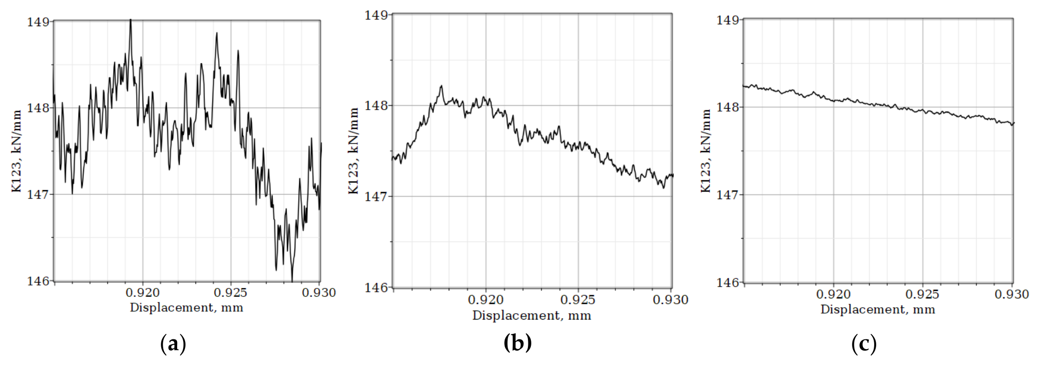

Table A1.
Excerpt from the recording of time, load, and displacement measurements.
| Time, s |
Load, kN |
Displacement, mm |
| 277,51 | 82,558 | 0,92503 |
| 277,52 | 82,562 | 0,92506 |
| 277,53 | 82,565 | 0,92509 |
| 277,54 | 82,569 | 0,92513 |
| 277,55 | 82,573 | 0,92516 |
| 277,56 | 82,577 | 0,92519 |
| 277,57 | 82,581 | 0,92523 |
| 277,58 | 82,584 | 0,92526 |
| 277,59 | 82,588 | 0,92529 |
| 277,60 | 82,591 | 0,92533 |
| 277,61 | 82,595 | 0,92536 |
| 277,62 | 82,599 | 0,92539 |
| 277,63 | 82,603 | 0,92543 |
| 277,64 | 82,607 | 0,92546 |
| 277,65 | 82,610 | 0,92549 |
| 277,66 | 82,614 | 0,92553 |
| 277,67 | 82,617 | 0,92556 |
| 277,68 | 82,621 | 0,92559 |
| 277,69 | 82,624 | 0,92563 |
| 277,70 | 82,628 | 0,92566 |
| 277,71 | 82,631 | 0,92569 |
| 277,73 | 82,640 | 0,92576 |
| 277,74 | 82,644 | 0,92579 |
| 277,75 | 82,648 | 0,92583 |
| 277,76 | 82,652 | 0,92586 |
| 277,77 | 82,656 | 0,92589 |
| 277,78 | 82,659 | 0,92593 |
| 277,79 | 82,663 | 0,92596 |
| 277,80 | 82,667 | 0,92599 |
| 277,81 | 82,670 | 0,92603 |
References
- Luo, H. F.; Tang, Y.; Feng, W. T.; Liu, J. F.; Li, H.; Zhou, E. Z. Progress in the application of DIC technology to rock mechanics testing: a review. Bull. Eng. Geol. Environ. 2025, 84, 628. [Google Scholar] [CrossRef]
- Hudson, J.A.; Crouch, S.L.; Fairhurst, C. Soft, Stiff and Servo-Controlled Testing Machines: A Review with Reference to Rock Failure. Eng. Geol. 1972, 6, 155–189. [Google Scholar] [CrossRef]
- Cai, M.; Hou, P.Y.; Zhang, X.W.; Feng, X.T. Post-peak Stress–Strain curves of brittle hard rocks under axial-strain-controlled loading. Int. J. Rock Mech. Min. Sci. 2021, 147, 104921. [Google Scholar] [CrossRef]
- Hou, P.Y.; Cai, M. Post-peak stress-strain curves of brittle hard rocks under different loading environment system stiffness. Rock Mech. Rock Eng. 2023, 55, 3837–3857. [Google Scholar] [CrossRef]
- He, H.; Xiao, Z.; Yang, Z.; Sun, T.; Ma, B.; Zhou, X.; Guo, T.; Wang, W.; Fang, J. Error in compression stress-strain curve recording without extensometer and its correction method for non-standard small-sized specimens. J. Strain Anal. Eng. Des. 2026, 61(1), 32–49. [Google Scholar] [CrossRef]
- Liu, W.; Huan, Y.; Dong, J.; Dai, Y.; Lan, D. A correction method of elastic modulus in compression tests for linear hardening materials. MRS Commun. 2015, 5(4), 641–645. [Google Scholar] [CrossRef]
- Hockett, J. E.; Gillis, P. P. Mechanical testing machine stiffness: Part I—Theory and calculations. Int. J. Mech. Sci. 1971, 13(3), 251–264. [Google Scholar] [CrossRef]
- Clarke, D.; Hinton, C. Adaptive Control of Materials-testing Machines. Automatica 1997, 33, 1119–1131. [Google Scholar] [CrossRef]
- Abdelaziz, A.; Grasselli, G. How believable are published laboratory data? A deeper look into system-compliance and elastic modulus. J. Rock. Mech. Geotech. Eng. 2021, 13, 487–499. [Google Scholar] [CrossRef]
- Bieniawski, Z.T. Mechanism of brittle fracture of rock: Part II—Experimental studies. Int. J. Rock Mech. Min. Sci. Geomech. Abstr. 1967, 4, 407–423. [Google Scholar]
- Eberhardt, E.; Stead, D.; Stimpson, B. Quantifying progressive pre-peak brittle fracture damage in rock during uniaxial compression. Int. J. Rock Mech. Min. Sci. 1999, 36, 361–380. [Google Scholar] [CrossRef]
- Briševac, Z.; Pollak, D.; Maričić, A.; Vlahek, A. Modulus of Elasticity for Grain-Supported Carbonates—Determination and Estimation for Preliminary Engineering Purposes. Appl. Sci. 2021, 11, 6148. [Google Scholar] [CrossRef]
- Jiang, Z.; Zhu, Z.; Accornero, F.; Lacidogna, G. Acoustic emission and digital image correlation evidence of size effects on the compression failure of concrete. Mag. Concr. Res. 2025, 77, 1060–1072. [Google Scholar] [CrossRef]
- Cai, M. Are there Class II rocks? J. Rock Mech. Geotech. Eng. 2025, 17(12), 7489–7502. [Google Scholar] [CrossRef]
- Arash, M.; Dolatshahi, A.; Molladavoodi, H.; Farrokh, E. Data-driven prediction of pure mode I fracture toughness in cementitious geomaterials using hybrid ANN–metaheuristic models. In Geomech. Geophys. Geo-energ. Geo-resour.; 2026. [Google Scholar] [CrossRef]
- Seferoğlu, M.T.; Aksüt, Y.S.; Seferoğlu, A.G. Flexural Behavior and Sustainability of Dual-Waste Fiber-Reinforced Concrete Designed for Pavement Applications. Buildings 2025, 15, 3454. [Google Scholar] [CrossRef]
- Narimani, S.; Davarpanah, S.M.; Kovács, L.; Vásárhelyi, B. Variation of Elastic Stiffness Parameters of Granitic Rock during Loading in Uniaxial Compressive Test. Appl. Mech. 2023, 4, 445–459. [Google Scholar] [CrossRef]
- Lv, L.; Yin, E.; Liu, X.; Wu, K. Energy-Based Evaluation of Brittleness in Moderately Weathered Rocks Under Triaxial Compression. Civ. Eng. J. 2026, 12(4), 1379–1397. [Google Scholar] [CrossRef]
- Li, J.; Liang, C.; Zhang, M.; Tan, G.; Wang, S. A FEM-informed BPNN surrogate model for asphalt pavement response prediction: toward an efficient computational module for digital-twin-oriented pavement management. Eng. Res. Express 2026, 8, 175109. [Google Scholar] [CrossRef]
- Koziel, S.; Pietrenko-Dabrowska, A.; Wojcikowski, M.; Pankiewicz, B. Efficient field correction of low-cost particulate matter sensors using machine learning, mixed multiplicative/additive scaling and extended calibration inputs. Sci. Rep. 2025, 15, 18573. [Google Scholar] [CrossRef]
- Wang, H.; Hu, J.; Gao, T.; Su, H.; Liu, S.; Liu, X. Evolution of the Young’s Modulus of Al-7Si-4Cu Alloy with Increasing Temperature by Various Strengthening Approaches. Materials 2026, 19, 1831. [Google Scholar] [CrossRef]
- Ahnert, K.; Abel, M. Numerical differentiation of experimental data: Local versus global methods. Comput. Phys. Commun. 2007, 177, 764–774. [Google Scholar] [CrossRef]
- Qin, Y.; Lang, L.; Tian, S.; Wu, T.; Tang, H.; Xu, J.; Zhang, Y.; Wang, J.; Lu, H.; Zhu, Z. Characteristics of Impact Fragmentation and Energy Dissipation of Cylindrical Rock Specimens with Various Aspect Ratios. Rock. Mech. Rock. Eng. 2025, 58, 6233–6254. [Google Scholar] [CrossRef]
- Alsaleh, S.; Abdelkarim, Y.; Mohamed, O. A critical review of BFRP-Reinforced concrete beam performance: failure mechanisms, design considerations, code provisions, and experimental–numerical correlations. J. Asian Archit. Build. Eng. 2026, 1–41. [Google Scholar] [CrossRef]
- Kolesnikov, G.; Shekov, V. Estimation of the Elastic Modulus of Granite Under Uniaxial Compression at the Pre-Peak Stage Using the PROS Method for Approximating Experimental Data. Appl. Sci. 2026, 16, 2571. [Google Scholar] [CrossRef]
- Zhao, W.; Wang, L.; Zhang, Z.; Mirjalili, S.; Khodadadi, N.; Ge, Q. Quadratic Interpolation Optimization (QIO): A new optimization algorithm based on generalized quadratic interpolation and its applications to real-world engineering problems. Comput. Methods Appl. Mech. Eng. 2023, 417, 116446. [Google Scholar] [CrossRef]
- Li, S.; Yue, X.; Li, Q.; Peng, H.; Dong, B.; Liu, T.; Yang, H.; Fan, J.; Shu, S.; Qiu, F.; et al. Development and applications of aluminum alloys for aerospace industry. J. Mater. Res. Technol. 2023, 27, 944–983. [Google Scholar] [CrossRef]
- Aluminum grade D16. Available online: https://oboronspecsplav.ru/marochnik/alyuminiy-deformiruemyy-splav/d16/ (accessed on 28 08 2026).
- Trčková, J.; Živor, R.; Přikryl, R. Physical and mechanical properties of selected amphibolite core samples from the Kola Superdeep Borehole KSDB-3. Terra Nova 2002, 14(5), 379–387. [Google Scholar] [CrossRef]
- Chen, X.; Wheeler, J.; Liu, J.; Zhou, B.; Hou, C.; Shan, H. Microstructures and seismic properties of amphibolites along the southern Ailao Shan–Red River belt: Implications for Oligo-Miocene crustal deformation in the southeastern Tibetan Plateau. Geological Society of America Bulletin 2026. [Google Scholar] [CrossRef]
- Shelekhova, T.S.; Lavrov, O.B.; Rodionov, G.N. New data on postglacial seismic dislocations in the Fennoscandian Shield—Rusian Plate contact zone, Pudozh district, Karelia, Russia. Geodyn. Tectonophys. In Russian. 2025, 16(4), 0840. [Google Scholar] [CrossRef]
- Zueva, I.A.; Lukina, M.D.; Rodionov, G.N. Features of earthquakes in Karelia based on seismic data for the period 2000–2024. Geophys. Res. In Russian. 2026, 26(3), 43–60. [Google Scholar] [CrossRef]
- Kulikov, V. S.; Svetov, S. A.; Slabunov, A. I.; Kulikova, V. V.; Polin, A. K.; Golubev, A. I.; Gorkovets, V. Ya.; Ivashchenko, V. I.; Gogolev, M. A. The 1: 750 000 Geological map of the southeastern Fennoscandia: New approaches to compilation. Trans. Karelian Res. Cent. Russ. Acad. Sci. 2017, 2, 3–41. [Google Scholar] [CrossRef]
- Shchipansky, A.A. Tectonic Origin of the Belomorian Mobile Belt and Belomorian Eclogites (N‒E Baltic Shield). Geotecton. 2025, 59, 287–309. [Google Scholar] [CrossRef]
- Kolesnikov, G.; Shekov, V.; Gavrilov, T. Modeling the Influence of Non-Constant Poisson’s Ratio on Crack Formation Under Uniaxial Compression of Rocks and Concrete. Eng 2025, 6, 130. [Google Scholar] [CrossRef]
Figure 1.
(a) Loading of the testing machine with a ball support but without a specimen; (b) loading with a specimen; (c) curves representing the behavior of the system without a specimen (12) and the system with a specimen (123).
Figure 1.
(a) Loading of the testing machine with a ball support but without a specimen; (b) loading with a specimen; (c) curves representing the behavior of the system without a specimen (12) and the system with a specimen (123).
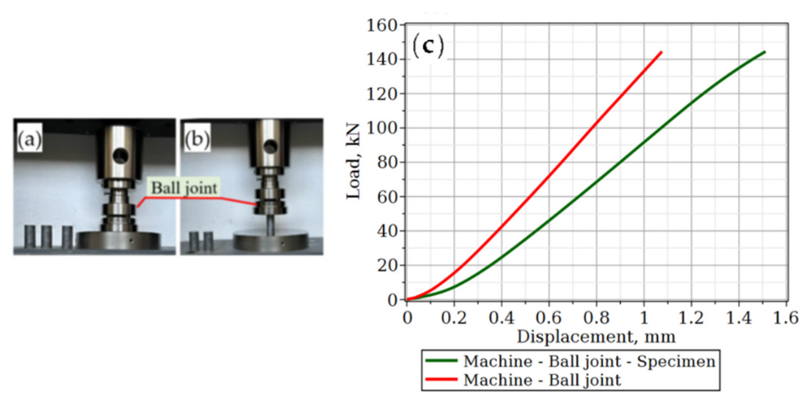
Figure 2.
The total displacement u123) is equal to the sum of the displacements resulting from the compliance of the “machine–ball joint” system u12) and the compliance of the specimen (u3). To determine the maximum value of the elastic modulus, a tangent is drawn to the “machine–ball joint–specimen” system curve at the point corresponding to the load P = P123, at which the stiffness of this system (K123) reaches its maximum. At the same load P = P123 = P12, the corresponding point on the “machine–ball joint” system curve and the tangent to that curve are determined.
Figure 2.
The total displacement u123) is equal to the sum of the displacements resulting from the compliance of the “machine–ball joint” system u12) and the compliance of the specimen (u3). To determine the maximum value of the elastic modulus, a tangent is drawn to the “machine–ball joint–specimen” system curve at the point corresponding to the load P = P123, at which the stiffness of this system (K123) reaches its maximum. At the same load P = P123 = P12, the corresponding point on the “machine–ball joint” system curve and the tangent to that curve are determined.
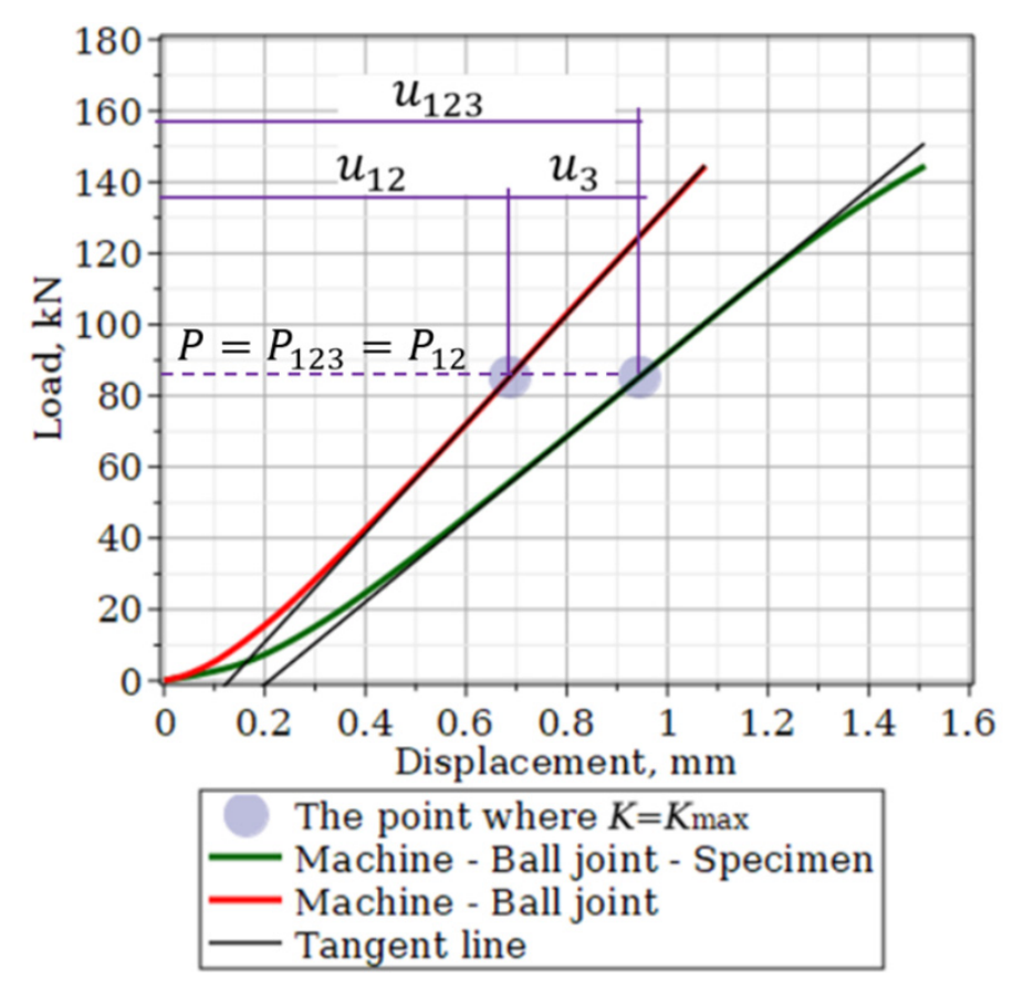
Figure 3.
Load–displacement curves for the “machine–ball assembly–specimen” and “machine–ball assembly” systems before and after correction. The circles indicate the points corresponding to the load P = P123 = P12, at which the stiffness coefficient of the “machine–ball assembly–specimen” system (K123) is at its maximum.
Figure 3.
Load–displacement curves for the “machine–ball assembly–specimen” and “machine–ball assembly” systems before and after correction. The circles indicate the points corresponding to the load P = P123 = P12, at which the stiffness coefficient of the “machine–ball assembly–specimen” system (K123) is at its maximum.
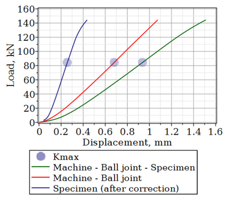
Figure 4.
(a) Amphibolite specimens; (b) specimen in the testing machine; (c) typical curves for amphibolite under compression testing. Load–displacement curves for the “machine–ball joint” and “machine–spherical assembly” systems before and after correction. Circles indicate points corresponding to the load P = P123 = P12, at which the stiffness coefficient of the “machine–ball joint–specimen” system (K123) is at its maximum.
Figure 4.
(a) Amphibolite specimens; (b) specimen in the testing machine; (c) typical curves for amphibolite under compression testing. Load–displacement curves for the “machine–ball joint” and “machine–spherical assembly” systems before and after correction. Circles indicate points corresponding to the load P = P123 = P12, at which the stiffness coefficient of the “machine–ball joint–specimen” system (K123) is at its maximum.
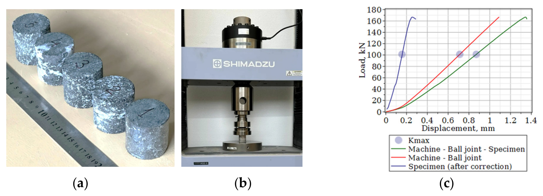
Table 1.
Input data and calculation results for the corrected stiffness coefficient and modulus of elasticity of an aluminum specimen.
Table 1.
Input data and calculation results for the corrected stiffness coefficient and modulus of elasticity of an aluminum specimen.
| Specimen | D mm |
L mm |
P123 kN |
u123 mm |
u12 mm |
u3 mm |
K3 kN/mm |
kN/mm |
Ecorrected GPa |
|---|---|---|---|---|---|---|---|---|---|
| Aluminum alloy (D16T) [28] | 23.6 | 51.0 | 84.4 | 0.937 | 0.677 | 0.260 | 324.4 | 648.8 | 75.6 |
Table 2.
Initial, intermediate, and derived data for determining the stiffness coefficient and modulus of elasticity of amphibolite.
Table 2.
Initial, intermediate, and derived data for determining the stiffness coefficient and modulus of elasticity of amphibolite.
| Specimen | No. | D mm |
L mm |
P123 kN |
u123 mm |
u12 mm |
u3 mm |
K3 kN/mm |
kN/mm |
Ecorrected GPa |
|---|---|---|---|---|---|---|---|---|---|---|
| Amphibolite (Avrios deposit) | 1 | 41.6 | 41.7 | 80.13 | 0.808 | 0.593 | 0.215 | 372.7 | 745.4 | 23.0 |
| 2 | 41.6 | 41.5 | 74.85 | 0.713 | 0.563 | 0.150 | 498.6 | 998.0 | 30.6 | |
| 3 | 41.6 | 41.6 | 99.10 | 0.854 | 0.700 | 0.154 | 639.3 | 1287.0 | 39.6 | |
| 4 | 41.6 | 41.5 | 61.18 | 0.680 | 0.486 | 0.194 | 313.7 | 630.7 | 19.4 | |
| 5 | 41.6 | 41.6 | 101.09 | 0.870 | 0.711 | 0.159 | 632.1 | 1271.6 | 39.1 | |
| Average | ||||||||||
| 41.6 | 41.6 | 83.27 | 0.785 | 0.61 | 0.1744 | 493.3 | 986.5 | 30.3 | ||
| Coefficient of variation, % | ||||||||||
| 0.0 | 0.0 | 16.2 | 9.0 | 12.4 | 13.8 | 24.2 | 24.2 | 24.2 | ||
Disclaimer/Publisher’s Note: The statements, opinions and data contained in all publications are solely those of the individual author(s) and contributor(s) and not of MDPI and/or the editor(s). MDPI and/or the editor(s) disclaim responsibility for any injury to people or property resulting from any ideas, methods, instructions or products referred to in the content. |
© 2026 by the authors. Licensee MDPI, Basel, Switzerland. This article is an open access article distributed under the terms and conditions of the Creative Commons Attribution (CC BY) license.
Copyright: This open access article is published under a Creative Commons CC BY 4.0 license, which permit the free download, distribution, and reuse, provided that the author and preprint are cited in any reuse.