

Submitted:
30 October 2026
Posted:
02 November 2026
You are already at the latest version
Abstract
The increasing use of lightweight, large compliant thin-walled structures (LCTS) made of carbon-fiber-reinforced polymer (CFRP) in aircraft fuselage assemblies contributes significantly to fuel efficiency and emission reduction. However, the low bending stiffness and large dimensions of these components make them highly susceptible to elastic deformation under gravity, fixture contact forces, and handling loads, so the geometry observed during manufacturing, inspection, and assembly does not represent the intrinsic, stress-free shape of the component. Because this gravity-free shape cannot be measured directly, it must instead be approximated from measurements taken under known loading conditions, combined with a numerical model of the component's structural response -- a separation that is required for reliable geometric inspection, digital assembly simulation, variation analysis, and fixture design. Minimal-contact supports commonly used for this purpose cause excessive deflection in structures of this size, while conventional multi-point supports leave the force distribution at each support point unknown, introducing ambiguity into the gravity compensation. This work addresses both limitations with a smart fixture system whose instrumented actuators render the imposed displacements and support states fully known, enabling a controlled, over-constrained support condition without loss of traceability of the applied loads. Surface measurements acquired on this fixture are combined with finite element simulations of the same loading configurations to approximate the gravity-free shape of large compliant CFRP structures, isolating manufacturing deviations from gravity-induced elastic deformation and yielding a gravity-free description of the component suitable for downstream geometric evaluation.
Keywords:
ixtures
; simulation
; metrology
; large compliant thin-walled structures
; carbon fiberreinforced polymer
; gravity-free shape estimation
1. Introduction
The assembly of aircraft fuselages and other lightweight airframe structures relies on large compliant thin-walled structures (LCTS) made of carbon fiber-reinforced polymers (CFRP). CFRP offers high strength and stiffness relative to its mass, making it suitable for lightweight load-carrying aircraft structures [1]. Stiffened CFRP panels are used in fuselages, rudders, and stabilizers, with representative fuselage designs combining a thin composite skin and reinforcing stringers [2].
Despite these material advantages, the low bending stiffness and large dimensions of these components make them susceptible to elastic deformation under gravity, fixture contact forces, and handling loads [3,4]. The geometry observed during manufacturing, inspection, and assembly therefore depends on both the manufactured shape and the loading conditions imposed during measurement. The measured surface contains manufacturing deviations together with reversible deformation, which cannot be separated through direct comparison with the nominal geometry alone.
These effects are also relevant to aircraft assembly, where part-to-part gaps depend on component deviations and the constraints applied during joining. To account for the effect of component shape variation on these gaps, Zaitseva et al. models initial-gap distributions for wing assembly analysis and applies the model to fastening-pattern optimization [5]. Where shims are required, conventional fitting may involve repeated gap measurement, component repositioning, and shim fitting. Measurement-driven simulation and sparse sensing have been investigated to reduce this effort by predicting gap distributions from measured geometry or historical production data [6,7]. These applications motivate a geometric description that can be transferred from the measurement setup to the intended assembly configuration.
Knowledge of the gravity-free shape (GFS), defined here as the component geometry in the absence of gravitational and externally applied loading, provides a reference for separating these effects. The GFS retains manufacturing deviations and is therefore distinct from the nominal design geometry. It also differs from the free state, which includes gravity-induced deflection, as discussed in Section 2. For inspection, this distinction enables the estimated manufacturing deviations to be evaluated separately from the elastic effects of the measurement setup [8,9]. For parts whose tolerances are specified under restraint, conformance must be assessed under those conditions rather than from the GFS alone [10].
Beyond inspection, component geometry and the intended support and joining conditions form the input to digital assembly simulations [11]. Grégorio et al. incorporate measured as-built geometry into a digital twin so that subsequent assembly operations can be adapted to the observed deviations [12]. For adaptive tooling, Neitmann et al. demonstrate closed-loop fixture adjustments that compensate for manufacturing tolerances and gravity effects during the assembly of compliant aircraft structures [4]. An estimated GFS supplies an unloaded geometric description for such models and compensation strategies. Gap prediction and tooling optimization remain downstream applications and are outside the scope of the present study.
The GFS cannot be measured directly in a conventional production environment and must instead be approximated from measurements and a numerical model of the component’s structural response. The correspondence between experimental support conditions and numerical boundary conditions is therefore critical. Minimal-contact supports may permit excessive deflection of a large compliant panel, whereas additional supports stabilize the measurement configuration but introduce further fixture interactions [13]. For CFRP, the model must also represent the directional material response [2].
This work presents a methodology for approximating the GFS of a large compliant CFRP fuselage panel measured on an instrumented multi-point smart fixture. Structured-light surface measurements are combined with anisotropic finite element (FE) simulations under corresponding actuator displacement inputs and support states. After rigid registration, the residual differences between the measured and simulated loaded geometries are interpreted as estimates of manufacturing deviations under the adopted modeling assumptions. The estimated deviation field is transferred onto the nominal geometry to reconstruct the unloaded manufactured shape. Consistency is assessed by comparing the reconstructed geometries and deviation fields across measurement configurations.
The remainder of this paper is organized as follows. Section 2 reviews existing approaches for GFS approximation. Section 3 introduces the proposed workflow. Section 4 describes the metrology system and communication architecture used for data acquisition. Section 5 presents the numerical simulation framework. Section 6 details the processing pipeline. Section 7 reports the results and validation. Section 8 concludes the work and outlines future directions.
2. Related Work
2.1. Terminology
Two related but distinct concepts appear in the literature on compliant part geometry and require clarification.
ISO 10579:2010, the standard on geometrical product specifications (GPS) for non-rigid parts, defines a non-rigid part as one that deforms to an extent that in the free state is beyond the dimensional and/or geometrical tolerances on the drawing [10]. The classification is therefore not an intrinsic material or structural property, but relative to the tolerances specified by the design engineer: the same component may be considered rigid under loose tolerances and non-rigid under tight ones. The standard defines the free state as the condition in which such a part is subjected only to the force of gravity, with no external constraints beyond a minimal support arrangement. The free state therefore includes gravity-induced elastic deformation and represents the shape a component assumes when resting under its own weight. The standard further requires that the orientation of the part with respect to the gravity vector is clearly defined, as different orientations produce different free-state geometries for the same component. A practical challenge in realizing the free state lies in the requirement that the support arrangement must not over-constrain the structure, i.e., apply more supports than the minimum needed to remove rigid-body motion, which would leave the contact force distribution statically indeterminate and introduce unknown deformation; for large compliant components, achieving a statically determinate support that does not itself introduce deformation is difficult to guarantee [14]. Schmitt et al. review the broader field of large-scale metrology and identify the non-linear growth of measurement uncertainty with part size as a fundamental challenge, noting that concepts such as virtual measuring processes are required once conventional fixture-based approaches reach their practical limits [15].
Both ISO 10579 and ASME Y14.5-2009 require that the geometry of a non-rigid part is assessed in a defined restraining condition, typically using a dedicated fixture that forces the part into a specified shape [10,16]. This fixture-based approach introduces an inherent bias: the measured geometry reflects one particular load configuration, while the same component may undergo substantially different loading conditions during assembly, where contact forces, clamp sequences, and gravitational orientation differ from those imposed by the inspection fixture. The assessed geometry is therefore not representative of the shape the part is expected to exhibit under actual operating conditions. For large compliant structures, this discrepancy can be significant, as the deformation response is sensitive to the number, location, and magnitude of the applied constraints.
Abenhaim et al. provide an early classification of non-rigid parts for inspection purposes, distinguishing components by the nature and magnitude of their compliant behavior and identifying the principal sources of shape variation, including gravity, residual stress, and fixture-induced deformation [14]. Makris et al. extend this with a broader dimensional classification in the context of automated assembly, categorizing compliant structures into one-, two-, and three-dimensional classes [17]. Within this framework, the CFRP fuselage panel considered in this work is a two-dimensional shell structure, where the thickness is negligible relative to the in-plane dimensions. The subsequent review of related work is scoped accordingly to approaches addressing two-dimensional compliant structures.
As introduced above, the gravity-free shape (GFS) denotes the component geometry under zero external loading, excluding gravitational self-weight. Claus et al. formalize this concept explicitly [18]. Unlike the free state, the GFS represents a hypothetical unloaded condition that cannot be observed directly in a production environment. As the condition of weightlessness is not reproducible on the shop floor, the GFS must be approximated, typically through a combination of measurement and finite element simulation [8,18]. The distinction between the free state and the GFS is maintained throughout this paper: the free state includes gravity, whereas the GFS excludes it.
2.2. Approaches for GFS Approximation
Abenhaim et al. categorize existing inspection strategies into two broad families: methods that require dedicated physical fixtures, and fixtureless methods that attempt to recover the unloaded geometry computationally [14]. This distinction provides the organizing framework for the four categories reviewed below: fixtureless geometric methods; measurement combined with FE simulation; reduced-order and surrogate methods, which accelerate the fixture-based family through pre-computed load-displacement relationships; and sensor-driven shape reconstruction, an alternative strategy that bypasses external geometric measurement altogether.
2.2.1. Fixtureless Geometric Methods
A first category of approaches recovers the unloaded shape from measurement data alone, without simulating loading conditions or requiring material property input. Radvar-Esfahlan and Tahan introduce Generalized Numerical Inspection Fixtures (GNIF) – despite the name, a purely computational technique requiring no physical fixture – which register measured and nominal shapes by exploiting the isometric invariance of geodesic distances under deformation, requiring no knowledge of material properties or boundary conditions [19,20]. Several subsequent works build on this fixtureless paradigm by incorporating finite element simulation into the registration pipeline: Sabri et al. refine displacement boundary conditions to improve profile inspection accuracy and later automate the full scan-to-deviation-map pipeline [21,22]; Sattarpanah Karganroudi et al. improve correspondence quality through registration-point filtering and validate robustness on aerospace panels [23,24]; and Babanezhad et al. propose a bi-criterion registration that simultaneously minimizes geometric distance and mechanical strain energy, improving defect detection for parts with significant free-state deformation [25]. Despite these advances, fixtureless methods remain limited to cases where the deformation between measured and nominal configurations is approximately isometric or can be captured by a simplified FE model. For large stiffened CFRP panels, where local stiffness varies significantly across the surface, these assumptions may not hold.
2.2.2. Measurement Combined with FE Simulation
The most extensively studied category couples physical measurements with finite element analysis to separate gravity-induced elastic deformation from manufacturing deviations. Lartigue et al. present an early framework combining photogrammetric acquisition with FE simulation to identify geometric deviations of flexible parts [26], and Thiebaut et al. extend this line of work by comparing measured data with simulated models to refine deviation predictions [8]. Gringoz et al. decompose the measured shape into a free-state geometry and configuration-dependent displacements computed via FE simulation, validating the approach on a composite nacelle component [27]. Lindau et al. scan parts resting on three well-defined support points to minimize external constraints, then apply gravity compensation using uniform isotropic material assumptions; while reasonable for automotive sheet metal, this approach may not generalize to composites, where deformation responses are direction-dependent [28]. Tuominen validates a virtual clamping approach on automotive production lines, demonstrating sub-millimeter agreement between simulated and physically clamped results, though the validation is restricted to welded steel assemblies with isotropic material behavior [29]. Claus et al. propose an iterative FEM-based procedure that inverts gravity-induced deformation starting from the measured loaded shape, with the key requirement that the measurement fixture must not over-constrain the part; otherwise, the contact force distribution becomes unknown and the gravity compensation yields ambiguous results [18]. Morse and Grohol propose an evaluation method based on superposition of gravity and fixturing effects pre-computed on the nominal geometry, enabling efficient estimation of both profile deviations and locating forces at fixture points, validated on an automotive fender with isotropic material assumptions [9].
A common limitation across these approaches is the reliance on isotropic, homogeneous material models and non-overconstrained fixtures, both of which become problematic for large anisotropic CFRP structures held in multi-point fixtures – precisely the combination addressed in this paper. Guo et al. review the specific challenges that arise in forced clamping and compensation processes for large integrated aeronautical composite structures, highlighting the need for methods that account for anisotropic stiffness and multi-point fixture interaction [30]. The present work addresses this gap by coupling structured-light scanning on an instrumented multi-point fixture with anisotropic FE simulation to approximate the GFS of a large CFRP fuselage panel.
2.2.3. Reduced-Order and Surrogate Methods
Rather than performing repeated full FE analyses, reduced-order methods pre-compute the relationship between loads and displacements to accelerate shape deviation evaluation. Maltauro et al. use the influence coefficient method to bridge the gap between design and manufacturing specifications for non-rigid parts, with pre-computed influence matrices relating applied forces to resulting displacements; the method is demonstrated on sheet metal parts with simple support conditions [31].
2.2.4. Sensor-Driven Shape Reconstruction
An alternative strategy bypasses external surface measurement entirely and reconstructs part geometry from embedded or attached sensors. Oboe et al. present a shape sensing methodology for a complex aeronautical structure using the inverse Finite Element Method (iFEM), reconstructing full-field displacements from local strain measurements without requiring material properties or external load information [32]. Given limited sensor coverage on the helicopter fuselage panel considered, they develop a simplified iFEM model incorporating geometric reductions and boundary condition tuning, validated both numerically and experimentally.
2.3. Research Gap and Positioning
Table 1 classifies the reviewed approaches along three axes: inspection strategy (fixtureless vs. fixture-based), fixture constraint level, and material assumption. The table highlights that existing methods either operate without fixtures under isometric or simplified FE assumptions, or rely on non-overconstrained fixtures with isotropic material models. No prior work addresses the combination of an overconstrained multi-point fixture with anisotropic composite material behavior, which is the setting addressed in this paper. An overconstrained, multi-point support is practically necessary for structures of this size: as discussed in the Introduction, minimal-contact supports lead to excessive deflection, while a multi-point layout keeps the panel in a repeatable, well-defined configuration for scanning. The present work resolves the resulting ambiguity in contact-force distribution by instrumenting each support point, and extends the anisotropic material treatment absent from prior fixture-based studies to account for the directional stiffness of CFRP.
3. Methodology
The gravity-free shape of a large CFRP fuselage panel is approximated from two data sources: surface measurements of the physical panel on an instrumented fixture, and a finite element simulation of the nominal panel under the same support and loading conditions. Figure 1 shows the test cell [33]: the panel rests on four actuators, each mounted on a force-torque sensor; a structured-light camera on a robot with a linear axis acquires the surface; and a laser tracker defines the global reference system. A second robot on a platform is part of the test cell but is not used in this study. The test cell and the calibration of the measurement chain are described in Section 4; the conceptual workflow is described below.
3.1. Definitions and Assumptions
Each shape is denoted by S with two labels: a superscript for its source – nominal (nom), measured (meas) or manufactured (man) – and a subscript for its physical state – free (free, unloaded), deformed under simulated external loading (def), or as configured for measurement on the fixture (conf).
The nominal free geometry represents the design intent without manufacturing deviations and without loads. Subjected in simulation to gravity and the support conditions of a configuration, it deforms to . The as-built panel measured on the fixture in the same configuration is , the stitched point cloud of that configuration. The aim is the GFS of the manufactured panel, , which contains the manufacturing deviations but no external loads.
The measured configuration is decomposed into an intrinsic deviation term and an external deformation term:
where is the displacement field due to manufacturing deviations and the deformation due to gravity and the supports. The latter is obtained from the FE simulation of the nominal geometry,
so that the manufacturing deviation follows as the residual between the measured and the simulated loaded shapes,
All three fields are evaluated along the normal of the nominal skin; tangential deviations are not determined (Section 7.6). The central assumption is that the FE model reproduces with sufficient fidelity. A rigid motion of the residual cannot be separated from the registration and is removed; a non-rigid error of the model remains in . The workflow therefore includes validations of the model that do not depend on the manufacturing deviation: the lift effect (the difference between two configurations, in which cancels) and the support forces. The synthetic benchmark of Section 7.4 quantifies how much of a model error the rigid registration passes into .
In this paper, the gravity-free shape denotes a geometry without gravity-induced deflection. This differs from the free state defined in ISO 10579:2010, which includes the effect of gravity [10].
3.2. Proposed Workflow
The workflow (Figure 2) combines an experimental and a numerical process in a hybrid pipeline. Process A stitches the captures of each configuration into with a calibrated measurement chain: a reference-ball calibration of the hand-eye transformation, followed by a correction of the hand-eye rotation and of a depth error of the camera estimated from the overlaps of the captures (Section 4.3). Process B simulates on the measured support positions under gravity and the actuator lifts of the configuration to obtain (Section 5). The hybrid pipeline (Section 6) then proceeds in four steps:
- 1.
- Rigid registration. The stitched cloud of the reference configuration is registered onto the undeformed FE surface: a coarse alignment from cylinder fits of the scan and of the model, without manually picked points, is refined by a robust rigid iterative closest point (ICP) algorithm, which alternately pairs each scan point with its closest point on the model and computes the rigid motion that minimises the weighted distances of these pairs. Since the laser tracker does not move during the campaign, the same transformation applies to all configurations.
- 2.
- Projection. Each scan point over the skin is projected onto the nominal skin, which gives its measured offset along the skin normal; the FE displacements of the configuration give the predicted offset at the same location.
- 3.
- Manufacturing deviation. The measured minus the predicted offset is the residual of Equation (3). Its best-fitting rigid motion, which absorbs the remaining registration error of the configuration, is removed; the remainder is of that configuration. Restricting this step to a rigid motion is intentional: a non-rigid alignment would also remove part of the manufacturing deviation.
- 4.
- Transfer and GFS. is transferred from the scan points to the nodes of the nominal skin as a barycentric-weighted mean and averaged over the configurations. Displacing the nominal skin by this mean along its normal gives .
Figure 3 shows the four steps on a section across the panel, with the data of configuration A1.
Three validations accompany the pipeline (dashed in Figure 2). Validation 1 compares the measured and the predicted lift effect, i.e. the difference between a configuration and the reference, in which and the registration cancel. Validation 2 compares the predicted support forces with the force-torque sensors. Validation 3 tests whether is the same in all configurations, as it should be if the model removes the external effects.
3.3. Design of Experiments
The design of experiments (Table 2) varies the support conditions of the panel to test whether the estimated manufacturing deviation is independent of them. A configuration is defined by the vertical lift of each actuator relative to the reference configuration. Each actuator is either at its reference height or lifted by 15 mm. A lift of one actuator twists the panel, which is supported at four points, and redistributes the support forces; the FE model has to reproduce both. The set comprises the reference, the four single lifts and three combined lifts, measured in this order; each configuration is captured with 128 scans (Section 4.2). In all configurations, the panel rests on the four actuators under gravity only; the suction grippers of the actuators are not used, so that no tensile support forces can be applied.
The actuators A1–A4 are shown in Figure 1 and Figure 8. They are 2599.4 mm apart along the panel and 1035.4 mm across it; the panel is about 3.5 m long and spans an arc of 60∘ at a nominal radius of 2000 mm (Section 4.1).
Each configuration yields a measured cloud and a corresponding FE simulation with the same lifts. Although the deformation differs between the configurations by 6–12 mm rms (Section 7.1), the manufacturing deviation of the panel does not change; the deviation fields estimated from the eight configurations are therefore expected to agree within the uncertainty of the measurement and of the model.
4. Metrology System
This section describes the test cell, the acquisition of the measurement data, and the calibration chain that turns the individual scans into one stitched point cloud of the panel with a quantified uncertainty. The test cell was introduced in previous work [33]; an overview is shown in Figure 1.
4.1. Experimental Setup
Existing approaches for GFS approximation typically require the measurement to be performed on a non-over-constrained fixture (Section 2), as the force distribution at additional support points is generally unknown and introduces ambiguity in the gravity compensation [18]. For large compliant structures, however, minimal support leads to excessive deflection and practical handling difficulties [17]. The test cell therefore supports the panel on four actuators, each mounted on a force-torque sensor that records the support load throughout the measurement. The support forces are thus not imposed but measured, and they are used to check the FE model (Section 7.1).
The panel is a stiffened CFRP fuselage panel covering one sixth of the circumference of the fuselage (an arc of 60∘ at a nominal radius of 2000 mm), about 3.5 m long, with eight hat stringers along its length. In the measurement campaign of this work, the panel had no frames. It rested on the four actuators A1–A4 (Figure 8) under gravity only; the suction grippers of the actuators were not used. The positions of the actuators were measured with the laser tracker on nests on the actuator plates: they are 1035.4 mm apart across the panel and 2599.4 mm along it. The inclination of each actuator head was measured on the scan of the reference configuration rather than with the inertial sensors of the actuators, which were not used: since the head plate lies flush on the skin, its inclination is that of the skin normal at the contact, obtained from a robust plane fit to the scan points within 50 mm of the contact point, in the levelled frame of the laser tracker. The heads are inclined by 15.2–16.0∘ to the vertical, across the panel. Each actuator is lifted by turning a rotary lever, and its stroke is read from a linear encoder on the actuator, so that the lift of every actuator is set and recorded at the fixture (the encoder measures the stroke of the actuator; a gap between the actuator and its seat reduces the lift received by the panel, Section 7.1); together with the measured support positions and the force-torque sensors, the imposed displacements and the support state of each configuration are thus known from measurement.
The panel geometry is captured by a Zivid 2+ MR60 structured-light camera carried by an ABB IRB 4600-40/2.55 industrial robot on a linear axis. A Leica T-MAC on the end effector is tracked by a Leica AT960 laser tracker, which defines the global reference system (GRS) and gives the pose of the end effector at each capture. The robot kinematics is not used for the stitching.
4.2. Acquisition
Each configuration of the panel is captured from 16 stations of the linear axis, 201 mm apart, with 8 robot poses per station along the curvature of the panel, i.e. 128 captures per configuration. Neighbouring stations overlap by about 62 %. After each move, the orchestration software waits 2 s; the laser tracker and the camera are then triggered simultaneously. For each capture, the raw point cloud of the camera (about 1.0–1.1 million points), the T-MAC pose measured by the tracker and the joint states of the robot are stored. All other sensor data, including the four force-torque sensors (about 500 Hz), are recorded continuously in a ROS 2 bag for the duration of the run. The software stack is built on ROS 2 [33]; the laser tracker is accessed through an HTTP server on the tracker computer.
A point of capture k, given in the camera frame, is transformed into the GRS by
where is the T-MAC pose measured by the tracker, the hand-eye transformation from the camera to the T-MAC, and denotes homogeneous coordinates. Since the raw clouds and poses are stored, every capture can be stitched again with a corrected or a corrected camera model. A recomputation of Equation (4) reproduces the clouds stitched online within 0.0003 mm.
4.3. Calibration Chain
The quality of the stitched cloud depends on the hand-eye transformation and on the camera itself. Both are calibrated in three steps: a reference-ball calibration before the campaign, and a correction of the hand-eye rotation and of a depth error of the camera estimated from the overlaps of the campaign itself (Figure 4). Before these steps, each raw cloud is cleaned in the camera frame.
4.3.1. Reference-Ball Calibration
The hand-eye transformation was calibrated against reference spheres at a fixed position: the camera measured a sphere of 66.62 mm diameter from 23 poses and a sphere of 97.14 mm diameter from 20 poses, and a least-squares fit gave and the sphere centres, a form of the hand-eye problem [34]. The combined fit has a residual of 0.368 mm rms. The two spheres alone give transformations that differ by 0.68 mm and 0.11∘, so the accuracy of is about mm and .
4.3.2. Cleaning of the Captures
Each raw cloud is cleaned in four stages before stitching: points outside a depth of 550–1000 mm are removed; a point is removed as noise if it lies more than 0.3 mm from a plane fitted to its 30 nearest neighbours or if it is isolated; points seen at more than 80∘ between the surface normal and the viewing ray are removed; and small disconnected clusters (DBSCAN on a 4 mm grid, less than 5 % of the points) are removed. Statistical outlier removal was not used: on these captures it removed 4–7 % of the points in bands on the steep stringer flanks, where the point density is lower but the points lie on the surface. The noise, grazing and cluster stages remove 0.31–0.39 % of the panel points in each run.
4.3.3. Hand-Eye Correction from the Overlaps
The overlaps of neighbouring captures measure the stitching error directly. For each pair of overlapping captures a and b, the signed distance
is evaluated between each point of b and its nearest point of a within 3 mm, along the normal ; its median is the offset of the pair. With the ball-calibrated , all 112–120 pairs of neighbouring stations in every run have a positive offset, with a median of 0.49–0.52 mm, whereas pairs of neighbouring poses at the same station are offset by only 0.08–0.11 mm. Between two captures of a station pair, only the linear axis moves; a constant offset of this kind is produced by a rotation error in the chain from the camera to the T-MAC: with a rail step of 201 mm, an error of 0.15∘ gives up to 0.53 mm.
A correction in the camera frame, , is therefore estimated by minimising the distances d of all neighbour pairs (Gauss–Newton with Huber weights). The translation of is not identifiable with eight poses and is not estimated. Fitted on each run alone, the rotation is the same in all eight runs (0.175–0.209∘, standard deviation of the components 0.003–0.011∘); fitted on all runs together, it is 0.194∘, about three times the accuracy of the ball calibration. A correction estimated on seven runs and applied to the eighth (leave-one-out) reduces the offset of its station pairs from 0.49–0.52 mm to to mm.
4.3.4. Depth Error of the Camera
After the hand-eye correction, a plane fitted to the distances d of each pair still reduces their robust standard deviation from 0.33 to 0.25 mm: a large part of the remaining disagreement is a slope. A random tilt of each capture would make the slopes of consecutive station pairs, which share one capture, negatively correlated (about ); the observed correlation is and for the two slope components. The slope is thus fixed in the image, i.e. a depth error of the camera that depends on the image position. It is modelled along the optical axis as
with the normalised image coordinates . Constant and linear terms are excluded, since the overlaps cannot distinguish them from a translation or a rotation of the camera. The true surface cancels in the distance of a point pair, which becomes linear in . Because the rotation and the cubic terms partly compensate each other (formal correlation up to 0.77), the 3 rotation parameters and the 7 coefficients are estimated jointly on all eight runs. The joint fit gives a rotation of 0.259∘ and a depth error of to mm over the image, largest at the image corners (Figure 5). Fitted on the four even runs and tested on the four odd runs, and vice versa, it reduces the robust standard deviation of d for the station pairs from 0.337 mm to 0.229–0.232 mm; the two halves agree.
4.4. Error Budget of the Stitching
The effect of each calibration step is quantified on all eight runs in three states: the original stitching with the ball-calibrated , the stitching with the hand-eye correction, and the stitching with the jointly estimated rotation and depth error (Figure 6). Two measures are used: the spread, i.e. the standard deviation between the captures that overlap in a cell of 5 mm, and a decomposition of the pair distances d. For the latter, the image of each capture is divided into cells; the point noise is the robust standard deviation of d about its mean in each pair-cell, and the pair-cell means are split, by a two-way analysis of variance components over 2694 pair-cells and the eight runs, into a part that repeats in every run and a part that changes from run to run.
The hand-eye correction removes the offset between stations; the spread drops from 0.36 to 0.20 mm, but the repeating part changes little. The depth-error correction removes most of the repeating part (0.28 to 0.075 mm) and reduces the spread to 0.135 mm (0.132–0.143 mm in the single runs). The part that changes from run to run stays at 0.05 mm through both steps, as expected for corrections that are the same in every run. After both steps, 71 % of the variance of d is point noise, 9 % changes from run to run and 20 % repeats.
The disagreement between captures grows with the number of captures that overlap in a cell (Figure 7), from 0.12 mm for 2 captures to 0.56 mm for 9 captures before the hand-eye correction, and to 0.10 and 0.34 mm after it.
4.5. Uncertainty of a Stitched Point
The standard uncertainty of a point of one capture, normal to the surface, is evaluated from the overlaps of the campaign (Type A evaluation [35]) and summarised in Table 3. The cell parts of the budget are divided by for one capture; the point noise is not, which makes the result conservative. The uncertainty of the correction itself is propagated by a Monte Carlo method [36]: 100 draws of the 10 parameters from their estimated covariance, each used to stitch the reference run again. The combined standard uncertainty of a point of one capture is 0.156 mm normal to the surface. Errors that are the same in all captures, such as errors of the laser tracker, the constant and linear terms of the depth error, the scale of the camera or the temperature, cannot be seen in the overlaps and are not included; their evaluation requires an independent reference.
The corrected captures of each run are merged and reduced to the mean of the points in cells of 2 mm. These clouds are the input of the processing pipeline (Section 6).
5. Simulation
This section describes the FE model that provides for each configuration of Table 2. The model is solved with ABAQUS/Standard.
5.1. Numerical Model Definition
The FE model of the nominal panel was supplied by the project partner as a ready-to-run ABAQUS model. It contains the curved skin and the eight stringers, tied to the skin; in agreement with the measured panel, no frames are included. The mesh consists of continuum-shell elements (SC8R, with SC6R in transition zones), 224,454 elements and 458,074 nodes in total. The skin is a laminate of 16 plies of 0.266 mm with the orientations . The ply material is linear-elastic and orthotropic (Table 4); its properties are estimates of the model supplier, as test data of the material were not available.
5.2. Supports and Loading
Each actuator is represented by a chain of connector elements from a reference point on the skin to a ground node. The reference point is coupled to the outer skin surface within a radius of 20 mm by a distributing coupling; the ground node is fixed. The influence of this and the other idealisations of the contact is assessed in Section 7.1. The connector chain carries the vertical support force, which is the quantity compared with the force-torque sensors.
The support positions are derived from the registered reference scan (Figure 8) (Section 6): the contact point and the skin normal of each actuator are taken from the scan, and the vertical is the vertical axis of the levelled laser tracker, which deviates by 3.3∘ from the z-axis of the model. Gravity and the actuator lifts act along this measured vertical. The actuator heads are inclined by 15.2–16.0∘ to the vertical (Figure 8).
Figure 8.
Panel and supports on the unrolled skin of the FE model: skin (light) and stringer surfaces (dark); contact points of the actuators A1–A4 as measured on the reference scan, with the inclination of the actuator head to the vertical.
Figure 8.
Panel and supports on the unrolled skin of the FE model: skin (light) and stringer surfaces (dark); contact points of the actuators A1–A4 as measured on the reference scan, with the inclination of the actuator head to the vertical.
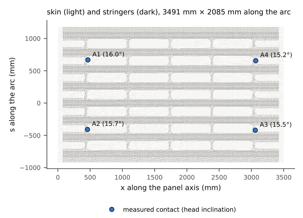
Two support behaviours are modelled. In the clamped model, the heads hold the panel in both directions. In the push-only model, the vertical connector of each actuator acts as a compression-only spring (104 N/mm), so that the panel can lift off an actuator, as it can on the fixture without suction. The two models are compared in Section 7.1.
In the plane of the actuator head, the heads are nearly free in the model (10 N/mm). On the fixture, the heads of A1, A2 and A4 were free in this plane, and the head of A3 was locked by a pin with a clearance of 0.5 mm. The in-plane slip of A3 in the model stays within this clearance in every configuration (at most 0.27 mm in the single lifts and 0.45 mm in A2+A4), so the pin does not engage, and A3 is modelled as free as well.
Each simulation has two steps. In the first, gravity is applied as a body force of 9810 mm/s2 to the skin and the stringers; geometric nonlinearity is accounted for (switching it off changes the shape by at most 0.11 mm, and by 0.34 mm in A2+A4; Table 5). In the second, the actuators lifted in the configuration are displaced by 15 mm along the vertical at their ground nodes. The reference configuration has the first step only.
5.3. Numerical Output Extraction
For each configuration, the nodal displacements at the end of the last step and the history of the connector forces are exported from the ABAQUS output database. The displacements of the outer skin surface give the predicted offset from the nominal geometry at each scan point (Section 6); the vertical connector forces give the support forces. A consistency check of all 16 simulations (eight configurations, two support models) confirms that the skin under each lifted actuator moves by the prescribed 15 mm within 0.05 mm, and that the sum of the support forces in the gravity step equals the weight of the model, 685.5 N (69.9 kg), in every simulation. In the push-only model of configuration A2+A4, the panel lifts off actuator A3 by 8.1 mm; in the clamped model of the same configuration, A1 and A3 carry tensile forces of and N.
6. Pipeline Implementation for GFS Approximation
This section describes the implementation of the hybrid pipeline of Section 3. Its inputs are the calibrated, merged point clouds of the eight configurations (Section 4.3) and the FE results of the corresponding simulations (Section 5). The pipeline is implemented in Python with Open3D [37]. One script runs all steps for all configurations and support models, from the corrected clouds to the figures of Section 7; the raw captures and the FE results are kept, so that every step can be repeated.
6.1. Registration
The cloud of the reference configuration is registered onto the outer surface of the undeformed FE model in two stages, without manually selected points. In the coarse stage, a robust cylinder fit to the scan and to the model gives for each the panel axis; together with the vertical, it defines a panel frame with its origin at the bottom of the trough, in the middle of the panel length. The bottom of the trough is used instead of the axis because the measured radius (2055 mm) differs from the nominal one; aligning the axes would leave the two surfaces apart by the difference of the radii. The scan frame is then turned about the axis so that the angular centres of the two panels, determined from their edges, coincide; without this roll, the subsequent ICP can converge one stringer pitch off. In the fine stage, a rigid ICP with Cauchy weights [38] refines the transformation on 1.8 million points. Since the laser tracker does not move during the campaign, this transformation is used for all eight configurations.
6.2. Projection and Deviation Field
Every second point of each registered cloud is projected onto the outer skin surface of the undeformed model. Whether a point belongs to the skin or to a stringer is decided on the deformed FE surface of its configuration, since a lifted skin comes close to the stringer flanks of the undeformed model; a point is kept if its closest triangle there is on the skin, within 15 mm. For each kept point i, the projection gives its foot point on the nominal skin, the barycentric coordinates of the foot point in its triangle, and the measured offset along the skin normal . The predicted offset at the same foot point follows from the nodal displacements of the FE simulation of the configuration, interpolated with the same barycentric coordinates and projected on the normal.
Points within 15 mm of a stringer or within 50 mm of the outline of the skin are excluded: there the scan mixes the skin with the stringer flanks or sees the panel edge, and the deviation is not consistent across the configurations (Section 7.3). The residual of configuration c at point i is
Its rigid part is the small rigid motion whose normal component best explains the residual in the least-squares sense,
with the foot points and their centroid . It absorbs the remaining registration error of the configuration and is removed; the remainder is the manufacturing deviation of configuration c.
6.3. Transfer to the Nominal Geometry and GFS
The deviation is transferred from the scan points to the nodes of the nominal skin as a mean weighted by the barycentric coordinates: each point contributes to the three nodes of its triangle with its barycentric weights ,
and nodes with a summed weight below 1 remain without a value. Unlike an assignment of each point to its dominant node, this mean uses all points in the neighbourhood of a node and does not depend on the order of the points.
At each node, a configuration whose value deviates by more than four robust standard deviations from the median of the configurations is rejected; this removes isolated artefacts that appear in single configurations only. The mean over the configurations, at nodes covered by at least five of the eight configurations, is the manufacturing deviation . This minimum excludes nodes that only a few configurations see, at which the deviation reflects these configurations rather than the panel (Section 7.2). The GFS is the nominal skin displaced by it along the nodal normals,
where are the nominal node coordinates; nodes without a value keep their nominal position.
7. Results and Validation
This section reports the results of the measurement campaign of Table 2: the reference configuration, four single lifts of 15 mm (A1, A2, A3, A4) and three combined lifts (A2+A4, A1+A4, A1+A2+A4), each scanned with 128 overlapping captures. With the stitching calibrated as described in Section 4.3, the FE model is first tested against the measured lift effects and the reaction forces; then the manufacturing deviation field and the resulting GFS are evaluated, including their consistency across the eight configurations.
7.1. Validation of the Structural Model
7.1.1. Lift Effect
The difference between a lifted configuration and the reference, both measured and both predicted, removes the as-built shape of the panel and the registration, which are common to both runs. It isolates the response of the panel to the actuator lifts, the part that the FE model has to reproduce. Figure 9 compares the measured and predicted lift effects on 20 mm cells. For the single lifts, the slope of the measured on the predicted lift effect is 0.98–1.13 and the correlation at least 0.994; the rms difference is 0.20–1.0 mm on lift effects of 6–7 mm rms. Over all seven lift cases (41,996 cells), the measured and predicted lift effects lie on the identity line.
7.1.2. Support Model
Two support models are compared in Figure 10, both at the measured support positions: heads that hold the panel in both directions (clamped) or only push it (push-only). After registration, both reproduce the absolute shape to 1.4–1.8 mm rms. They give the same result in every configuration except A2+A4, where the push-only model lets the panel lift off actuator A3 and almost unload A1 (8 N) and fails to reproduce the measurement (3.5 mm rms against 1.7 mm clamped). The clamped model is used in the following. In A2+A4, however, it predicts tensile forces at A1 and A3 ( and N), which heads that only push cannot apply; the measured forces at A1 and A3 decrease by 112 and 111 N, about half the predicted 228 N (Table 6). Neither model reproduces this configuration completely. Both observations are consistent with a smaller lift received at A4 than commanded (Section 7.1, Reaction Forces): with less twist imposed, the panel stays in contact with all four heads, and no tension arises. Accordingly, of A2+A4 differs most from the other configurations (0.25 mm rms against 0.12–0.23 mm, Section 7.3).
Sensitivity to the support idealisation. In the model, the support forces are not imposed: the lifts are prescribed displacements, and the forces follow from the stiffness of the panel. The influence of the idealised contact was tested in all eight configurations by varying it in three ways, each between two simulations that differ in this setting only (Table 5): (i) the vertical contact law, clamped or push-only heads; (ii) the in-plane contact of A3, locked in its plane ( N/mm), as its pin would act if it engaged, or free (10 N/mm); (iii) geometric nonlinearity, on or off, with clamped and with push-only heads. The table gives the change of the predicted shape that reaches , i.e. without its best-fitting rigid motion, and the largest change of a vertical support force. The in-plane lock changes the shape by at most 0.02 mm and the forces by at most 0.3 N. Geometric nonlinearity changes the shape by at most 0.11 mm and the forces by at most 1.4 N, except in A2+A4, the configuration with the largest twist (0.34 mm, 2.4 N, clamped). With push-only heads, its effect is the same in every other configuration and smaller in A2+A4 (0.21 mm, 0.1 N), where the panel lifts off A3; the small effect of the nonlinearity therefore does not depend on the contact law. The contact law matters only where the panel lifts off a head: in A2+A4, the push-only model changes the shape by 1.4 mm rms and the forces by up to 62 N; in all other configurations, by at most 0.02 mm and 0.3 N. Apart from the contact law in A2+A4, discussed above, all variations are small against the field (1.53 mm rms) and its spread over the configurations (median 0.17 mm). The radius of the coupling between head and skin (20 mm) was not varied. It distributes the support force over the contact patch and changes the deformation only near the head, whereas the resultant force, which the sensors measure, follows from the global stiffness of the panel. A compliant contact would moreover reduce the twist together with the force, which is not observed (below). Compared with these variations, the stiffness of the model is the dominant model uncertainty.
7.1.3. Reaction Forces
The lift effects test the deformed shape, but since the lifts are prescribed displacements, they do not test the stiffness of the model. The force-torque sensors of the four actuators provide this test. Table 6 compares the change of the support forces from the reference configuration, which cancels the sensor offsets and the weight of the actuator heads. The measured value is the axial force of each sensor; the orientations of the sensors were not measured (their lateral components are not aligned with each other), so the comparison with the vertical force of the model assumes that the sensor axes are close to vertical. Even a tilt by the inclination of the heads (16∘) would change the axial force by only 4 %, far less than the difference found below. The model reproduces the pattern of the load redistribution in every configuration: lifting one actuator loads its diagonal pair and unloads the other. The measured force changes, however, are 0.69–0.75 of the predicted ones for the single lifts. Since the deformation of the panel itself is reproduced (slope of the lift effect after removal of its rigid part 0.92–0.98), the measured force per unit twist is about 0.75 of the model in every configuration. A compliant contact at the actuator heads would reduce the twist together with the force and is therefore not the cause; the difference points to the torsional stiffness of the model or to the scaling of the sensors, which is decided below.
The combined lifts show a smaller ratio. Their lift effects show that the twist actually imposed on the panel was smaller than predicted (slope of the deformation part 0.69 for A2+A4 and 0.44 for A1+A2+A4), and relative to that twist the force ratio is again 0.70–0.77. For A1+A4, the model predicts no twist and no force change; the measured N and a small measured twist (0.26 mm rms) show that the two lifts were not equal in effect. All three combined configurations contain A4 and fall short of the sum of the corresponding single lifts by the same twist pattern (, and N in the order of measurement). A likely cause is that the foot of actuator A4 was no longer fully seated after the single lift of A4, so that part of its stroke closed a gap instead of lifting the panel; the FE model of the combined configurations then prescribes a larger lift at A4 than the panel received. The encoders cannot show this, since they measure the stroke of the actuator and not the lift received by the panel; the assessment of the stiffness therefore rests on the single lifts.
Whether the ratio of about 0.75 lies in the model or in the sensors was decided by weighing the panel with the sensors. The zero of each sensor was measured with its actuator head lowered clear of the panel, and the panel was supported on three of the four actuators. In two such states, the vertical forces of the three loaded sensors, less their zeros, sum to 682 and 660 N, i.e. 0.995 and 0.96 of the weight of the FE model (685.5 N). The sensor scale is therefore correct, and the FE model is about 25 % too stiff in torsion.
7.2. Manufacturing Deviation Field and GFS
For each configuration, the measured offset of the skin from the nominal geometry minus the offset predicted by the FE model (gravity and actuator lifts) is the part that the model does not explain. Its best-fitting rigid motion (0.84–1.43 mm rms) is attributed to the registration and removed; the remainder is of that configuration. Scan points within 15 mm of a stringer or within 50 mm of the outline of the skin are left out (Section 7.3). In addition, at each node, a value more than four robust standard deviations from the median of the configurations is rejected; this removes isolated artefacts that appear in single configurations (most in A2+A4, 2,927 values). The mean is formed on the nodes that at least five of the eight configurations cover (37,585 nodes). This rule leaves out 98 nodes (0.3 %), all at the far end of the panel, in a strip at the panel end and along the lower long edge. Most of them are covered only by the three combined configurations, all of which lift the far end with A4; there, points that do not belong to the skin come within the skin tolerance, and on 48 of these nodes reaches 5–16 mm. Since these configurations agree with each other, the rejection per node does not remove them. A deviation that appears only when one end of the panel is lifted is, however, a property of these configurations and not of the panel. With these nodes, the field would be 1.60 mm rms instead of 1.53 mm; for a minimum of four to six configurations it is 1.53 mm, so the choice of the threshold is not critical. is evaluated on 37,631–37,833 of the 126,527 skin nodes (30 %). The rest, grey in Figure 11, is left out for two different reasons. On 38 % of the skin nodes there is no measurement: the skin under the stringer feet and inside the hat stringers is hidden from the camera, and parts of the outline lie outside the scanned area. On a further 32 %, the scanner sees the skin, but within 15 mm of a stringer the scan mixes the skin with the stringer flanks, and within 50 mm of the outline it sees the panel edge and the stringer ends. There the residual changes from one configuration to the next far more than elsewhere (Section 7.3, Figure 13). It is then a property of the configuration rather than of the panel, which contradicts the definition of ; the margins therefore follow from the same consistency criterion that validates the field.
The GFS is not extended into these regions, neither by interpolation nor by the model. Under a stringer, the skin is stiffened by and joined to the stringer, so its deviation need not continue that of the neighbouring bays; an interpolated value would present an assumption as a measurement. The FE model describes only the nominal panel and carries no information on the manufacturing deviation. Where a complete geometry is needed, e.g. for assembly simulation, the GFS keeps the nominal geometry in these regions.
Figure 11a shows the mean of over the eight configurations. It is a smooth field of 1.53 mm rms (5–95 %: to mm): the middle of the arc lies up to about 3 mm further towards the panel axis than the nominal geometry, and the long edges up to about 4 mm further away from it, i.e. the panel is flatter than the nominal arc. The GFS, , is the nominal skin displaced by the mean along its normal.
7.3. Consistency Across Configurations
If the panel and the model behave as assumed, does not depend on the supports or the lifts. The standard deviation of over the eight configurations has a median of 0.17 mm per node and a 95th percentile of 0.33 mm (Figure 11b), against a field of 1.53 mm rms and lift effects of 6–12 mm rms that the model removes. Each configuration differs from the mean of the other seven by 0.12–0.25 mm rms, and the pairwise rms differences range from 0.06 to 0.39 mm (Figure 12a).
The differences are not random. The configurations pair up by diagonal: A1 and A3 agree to 0.06 mm, A2 and A4 to 0.10 mm, A1+A4 and A1+A2+A4 to 0.14 mm. Between the two diagonals, a smooth change of the arc curvature of about mm remains (Figure 12c), about 5 % of the lift effect. It is not a drift over the day, since the runs were measured in the order A1, A2, A3, A4. This remaining configuration dependence is therefore reported as such, rather than as part of a constant manufacturing deviation.
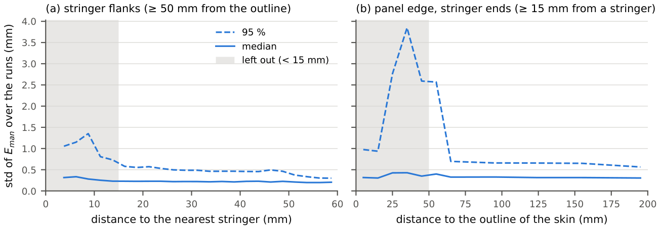
The margins at the stringers and at the outline follow from the same consistency criterion. Without them, the spread of over the configurations rises sharply towards the stringer flanks and the panel edge (Figure 13), where the scan mixes the skin with the flanks or sees the edge and the stringer ends. Beyond 15 mm from a stringer, the median spread no longer depends on the distance, while its 95th percentile continues to decrease slowly. At the outline, the 95th percentile remains high up to 55–60 mm, while the median is constant beyond 50 mm; the margin of 50 mm is kept, and the remaining edge effect affects only the upper tail of the spread.
Figure 12.
Consistency of across the configurations. (a) Rms of the pairwise differences; (b) distribution of the difference per node for the best, the median and the worst pair; (c) difference between configurations A1 and A2 on the unrolled skin.
Figure 12.
Consistency of across the configurations. (a) Rms of the pairwise differences; (b) distribution of the difference per node for the best, the median and the worst pair; (c) difference between configurations A1 and A2 on the unrolled skin.
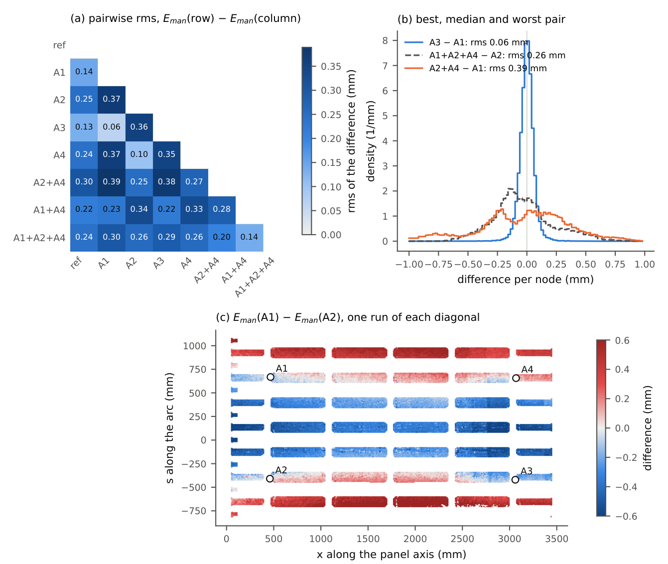
Figure 13.
Spread of over the configurations without removal of artefacts, against (a) the distance to the nearest stringer and (b) the distance to the outline of the skin. Shaded: left out.
Figure 13.
Spread of over the configurations without removal of artefacts, against (a) the distance to the nearest stringer and (b) the distance to the outline of the skin. Shaded: left out.
7.4. Synthetic Benchmark of the Pipeline
The consistency across configurations does not reveal errors that are common to all of them. A synthetic benchmark with a known manufacturing deviation gives the error of the pipeline itself and shows how much of a model error the rigid registration passes into (Figure 14). A known field , a smooth shape fitted to the measured with local bumps of mm and dips of mm at the actuators (1.42 mm rms), is added along the normal to the deformed surface of a truth FE model at the real scan points of each configuration, together with normal noise of 0.16 mm per point (Table 3) and a rigid error common to all configurations. The synthetic clouds pass through the unchanged pipeline, and the recovered is compared with on the evaluated skin nodes.
With the truth equal to the subtracted model, the pipeline recovers to 0.041 mm rms (95th percentile 0.085 mm, maximum 0.24 mm), about 3 % of the field (Figure 15); this is the error intrinsic to the algorithm. Without an injected field, noise and registration alone leave 0.016 mm rms. A support model in the truth that differs from the subtracted one (push-only against clamped) leaves the error unchanged (0.040 mm rms), and a registration error of 14 mm along the panel axis, the size of the difference between the measured and the design actuator positions, raises it to 0.046 mm rms. Tangential deviations, which move the skin and the stringers within the surface and carry and the gravity sag with the material, do not change it either: 0.042 mm rms for an in-plane shrinkage of 0.3 mm/m with stringers offset by mm, and 0.040 mm rms for a smooth tangential field of 2 mm rms (Section 7.6). A panel uniformly 25 % softer than the model, the size of the difference indicated by the reaction forces, biases the recovered field by 0.25 mm rms (95th percentile 0.46 mm, maximum 0.75 mm). This bias is nearly the same in every configuration (0.24–0.26 mm rms) and has the shape of a smooth change of curvature (Figure 15d); it is the dominant error of and the bound quoted in Section 7.6. The benchmark generates the synthetic scans with the model that the pipeline subtracts, perturbed only in the ways listed; model errors not perturbed here and spatially correlated errors of the stitching are not covered. The spread of over the measured configurations (median 0.17 mm per node, Section 7.3) is accordingly larger than the error of the pipeline alone: it contains the configuration-dependent errors of the model, such as the smaller lift received at A4 in the combined configurations and the remaining dependence on the diagonal ( mm), which the benchmark does not reproduce.
7.5. Discussion of Key Findings
Three results support the approximation of the GFS from measurements on an over-constrained fixture. First, the corrected stitching reduces the measurement error to 0.13 mm, well below the manufacturing deviations of the panel. Second, with the measured support positions, the FE model reproduces the measured response to the actuator lifts in shape and magnitude, in all seven lift configurations. Third, the manufacturing deviation field estimated from eight configurations with different supports and lifts agrees to 0.17 mm (median per node), an order of magnitude below the field itself and two orders below the lift effects.
The configurations change the measured support forces by up to 110 N per actuator and the shape of the panel by 6–12 mm rms. The consistency of across them is therefore a test of the workflow under substantially different load distributions. All configurations, however, keep the panel on four supports: they vary the loads, not the number of supports. A configuration with reduced constraint, e.g. on three supports, was not scanned and remains to be tested.
Consistency does not, however, prove correctness. An error that is the same in every configuration, such as an error of the gravity load or of the stiffness in the gravity step, enters identically in every run and cannot be detected by comparing configurations. The reaction forces are the only independent test of the stiffness in the present data, and they indicate a difference of about 25 % (Section 7.1).
7.6. Limitations and Uncertainty Conditions
The uncertainty sources of the workflow are summarized in Figure 16, and the quantified contributions in Table 7.
Combined uncertainty. The contributions are combined per node as independent standard uncertainties [35]: the spread of over the configurations (Type A), divided by rather than , since the configurations pair up by diagonal and are not independent repetitions; the systematic part of the stitching (0.053 mm) and the uncertainty of its correction (0.016 mm), which are the same in every configuration; the error of the pipeline from the synthetic benchmark (0.041 mm); and the bias from the stiffness of the model at each node, from the benchmark with a uniformly 25 % softer panel. The combined standard uncertainty of the GFS offset is 0.24 mm per node (median; 95th percentile 0.52 mm), i.e. an expanded uncertainty of 0.49 mm (), against a field of 1.53 mm rms (Table 7). The stiffness of the model dominates: without it, the combined uncertainty is 0.14 mm. Counting all eight configurations as independent would lower it only to 0.22 mm. Errors common to all captures, such as those of the laser tracker or of the scale of the camera, are not included, since the overlaps cannot reveal them.
Stiffness of the model. The force comparison, with the sensors checked against the weight of the panel, shows that the FE model is about 25 % too stiff in torsion. A model that is too stiff underestimates the gravity sag, and the difference enters in every configuration alike, so the consistency across configurations does not reveal it. If the whole model were 25 % too stiff, the synthetic benchmark (Section 7.4; panel 25 % softer than the subtracted model, full pipeline) recovers with an error of 0.25 mm rms (95th percentile 0.46 mm, at most 0.75 mm) on the evaluated skin, against a field of 1.53 mm rms; the rigid registration absorbs almost none of it, since the error is the non-rigid part of the additional gravity sag. This assumes a uniformly softer panel; since the forces test the torsional stiffness, which governs the gravity sag only in part, the actual bias is likely smaller. Identifying the stiffness of the panel from the measured forces and deformations would remove this bias.
Normal component only. is evaluated along the surface normal, and the GFS is the nominal skin displaced along its normal. On a smooth skin, the scan constrains only this component: a displacement of the surface within itself, such as an in-plane shrinkage of the laminate, does not change the measured geometry. Tangential manufacturing deviations are therefore neither measured nor contained in the GFS. They could only be observed at geometric features such as edges, stringer feet and holes, which are excluded from the evaluated area. Their effect on the normal field is small. The skin is a cylinder, so a tangential deviation changes its normal geometry only to second order, m for mm and mm. To first order, the gravity sag is subtracted at the nominal instead of the actual position of a material point; with the slope of the computed sag (at most 0.023 in all configurations), this changes the GFS by at most 0.05 mm for mm. In addition, each value of is attributed to the nominal position of its material point. This does not change the shape of the GFS but places its values up to away from the material they belong to, an error of at a material point: with the slope of the measured field (median 0.007), 0.013 mm in the median and 0.11 mm at the 95th percentile for mm, and 0.003 mm and 0.03 mm for mm. The synthetic benchmark confirms this (Section 7.4): an in-plane shrinkage of 0.3 mm/m with stringers offset by mm, and a smooth tangential field of 2 mm rms, leave the error of the recovered field at 0.042 and 0.040 mm rms (0.041 mm without), and change the error at the material points by less than 0.002 mm rms. The GFS is therefore suited to tasks governed by the normal shape of the evaluated skin, such as the contour of the skin bays; at the stringer feet and the edges, where the interfaces to the substructure lie, it remains nominal (coverage, below). It does not provide in-plane positions such as those of stringers, holes and trimmed edges; these require a measurement of the features, for which the scans of the stringer flanks and panel edges could be used.
Coverage. is evaluated on 30 % of the skin nodes (Section 7.2): the rest is not seen by the scanner (38 %) or lies within the margins, where the scan is not consistent across configurations (32 %). The GFS in these regions remains nominal. A smooth representation of fitted to the evaluated area could bridge the margins and the stringer feet, with an uncertainty that grows with the distance to the evaluated skin.
Rigid registration. The rigid motion fitted per configuration absorbs any error of the model that has a rigid component, together with the registration. Non-rigid model errors remain in . They are bounded by the consistency across configurations only if they change with the configuration, as discussed above.
8. Conclusions
This paper presented a workflow for approximating the gravity-free shape of a large compliant CFRP fuselage panel measured on an over-constrained, instrumented fixture. Structured-light scans, stitched with a calibrated measurement chain, are compared with FE simulations of the nominal panel on the measured supports; the residual, after removal of its rigid part, is the manufacturing deviation, and the nominal geometry displaced by it is the GFS. The workflow was applied to eight support configurations of one panel.
The main findings are:
- Calibration of the measurement chain. A reference-ball calibration of the hand-eye transformation left a systematic offset of 0.5 mm between neighbouring stations. A correction of the hand-eye rotation (0.19∘) and of a depth error of the camera, both estimated from the overlaps of the captures, reduces the spread between overlapping captures from 0.36 mm to 0.135 mm and the systematic part that repeats in every run from 0.34 mm to 0.075 mm. The combined uncertainty of a point of one capture is 0.16 mm normal to the surface.
- Validation of the FE model. With measured support positions, the model reproduces the measured response to the actuator lifts in all seven lift configurations (slope 0.98–1.13, correlation ≥ 0.966). Its deformation part, the twist of the panel, is reproduced in the single lifts; in the combined lifts the panel received 0.44–0.69 of the predicted twist, most likely because actuator A4 was not fully seated. The support forces show the predicted redistribution in every configuration, but about 25 % lower than predicted for the same deformation.
- Manufacturing deviation and GFS. The manufacturing deviation is a smooth field of 1.53 mm rms: the panel is flatter than the nominal arc. Estimated independently from the eight configurations, it agrees to a median of 0.17 mm per node, an order of magnitude below the field itself, although the deformation differs by 6–12 mm rms between the configurations.
The approach thus yields a repeatable GFS estimate from measurements on an over-constrained four-point fixture, where the support forces are measured rather than assumed. Its main limitations are the stiffness of the FE model, which the force comparison calls into question and which would bias the deviation in every configuration alike; the evaluation of the normal component only, so that the GFS does not provide the in-plane positions of stringers, holes or edges; the coverage of about 30 % of the skin nodes that the camera sees directly; and a remaining configuration dependence of about mm.
Future work should identify the stiffness of the panel from the measured forces and deformations, including a measurement of the sensor orientations; validate the stitched geometry against an independent reference; and extend the campaign to the suction grippers, which allow tensile support forces.
Author Contributions
Conceptualization, R.S. and A.M.; methodology, G.T. and M.H.R.; software, M.H.R. and G.T.; validation, M.H.R. and G.T.; formal analysis, M.H., G.T. and A.M.; investigation, M.H.R. and G.T.; resources, A.M. and R.S.; data curation, M.H.R. and G.T.; writing—original draft preparation, M.H.R. and G.T.; writing—review and editing, G.T., M.H. and A.M.; visualization, M.H.R. and G.T.; supervision, G.T., A.M., A.B. and R.S.; project administration, G.T., A.M. and R.S. All authors have read and agreed to the published version of the manuscript.
Funding
This research received no external funding.
Institutional Review Board Statement
Not applicable.
Informed Consent Statement
Not applicable.
Data Availability Statement
The data presented in this study are available on request from the corresponding author. The raw measurement data are not publicly available due to confidentiality restrictions imposed by the industrial project partner.
Acknowledgments
The authors would like to thank the project partners for providing the CFRP panel and the nominal FE model used in this study. The authors used the AI assistant Claude (Opus 5.5, Anthropic) to refactor and extend the analysis code, which the authors had initially written. The authors reviewed and verified all code and results and take full responsibility for the content of this publication.
Conflicts of Interest
The authors declare no conflicts of interest.
Abbreviations
The following abbreviations are used in this manuscript:
| l]@ll BC | Boundary Condition |
| CAD | Computer-Aided Design |
| CFRP | Carbon Fiber-Reinforced Polymer |
| DoE | Design of Experiments |
| FE | Finite Element |
| GFS | Gravity-Free Shape |
| GRS | Global Reference System |
| ICP | Iterative Closest Point |
| LCTS | Large Compliant Thin-walled Structure |
| RMS | Root Mean Square |
| ROS 2 | Robot Operating System 2 |
References
- Boni, L.; Fanteria, D.; Lanciotti, A. Post-buckling behaviour of flat stiffened composite panels: Experiments vs. analysis. Compos. Struct. 2012, 94, 3421–3433. [Google Scholar] [CrossRef]
- Bouslama, N.; Maslouhi, A.; Masson, P. Experimental and numerical investigation of damage evolution in carbon fiber reinforced polymer stiffened panel in post-buckling regime. J. Compos. Mater. 2022, 56, 2455–2470. [Google Scholar] [CrossRef]
- BAO, Y.; WANG, B.; HE, Z.; KANG, R.; GUO, J. Recent progress in flexible supporting technology for aerospace thin-walled parts: A review. Chin. J. Aeronaut. 2022, 35, 10–26. [Google Scholar] [CrossRef]
- Neitmann, M.; Rothe, T.; Kappel, E.; Hühne, C. Assembly of Compliant Structures with Autonomous Industrial Mobile Manipulators (AIMM) Using an End Effector with Active Deformation Compensation for the Assembly of Flaps. Machines 2022, 10, 291. [Google Scholar] [CrossRef]
- Zaitseva, N.; Lupuleac, S.; Shinder, J. Initial gap modeling for wing assembly analysis. In Aerospace Systems; 2024. [Google Scholar] [CrossRef]
- Esposito, C.; Cosenza, C.; Gerbino, S.; Martorelli, M.; Franciosa, P. Virtual shimming simulation for smart assembly of aircraft skin panels based on a physics-driven digital twin. Int. J. Interact. Des. Manuf. (IJIDeM) 2022, 16, 753–763. [Google Scholar] [CrossRef]
- Manohar, K.; Hogan, T.; Buttrick, J.; Banerjee, A.G.; Kutz, J.N.; Brunton, S.L. Predicting shim gaps in aircraft assembly with machine learning and sparse sensing. J. Manuf. Syst. 2018, 48, 87–95. [Google Scholar] [CrossRef]
- Thiébaut, F.; Lacroix, C.; Andolfatto, L.; Lartigue, C. Evaluation of the shape deviation of non rigid parts from optical measurements. Int. J. Adv. Manuf. Technol. 2016, 88, 1937–1944. [Google Scholar] [CrossRef]
- Morse, E.; Grohol, C. Practical conformance evaluation in the measurement of flexible parts. CIRP Ann. 2019, 68, 507–510. [Google Scholar] [CrossRef]
- ISO 10579:2010; Geometrical product specifications (GPS) — Non-rigid parts — Dimensioning and tolerancing. International Organization for Standardization: Geneva, 2010.
- Lupuleac, S.; Zaitseva, N.; Stefanova, M.; Berezin, S.; Shinder, J.; Petukhova, M.; Bonhomme, E. Simulation of the Wing-to-Fuselage Assembly Process. J. Manuf. Sci. Eng. 2019, 141, 061009. [Google Scholar] [CrossRef]
- Grégorio, J.L.; Lartigue, C.; Thiébaut, F.; Lebrun, R. A digital twin-based approach for the management of geometrical deviations during assembly processes. J. Manuf. Syst. 2021, 58, 108–117. [Google Scholar] [CrossRef]
- Liu, C.; Wang, J.; Zhou, B.; Yu, J.; Zheng, Y.; Liu, J. Development of Fixture Layout Optimization for Thin-Walled Parts: A Review. Chin. J. Mech. Eng. 2024, 37. [Google Scholar] [CrossRef]
- Abenhaim, G.N.; Desrochers, A.; Tahan, A. Nonrigid parts’ specification and inspection methods: notions, challenges, and recent advancements. Int. J. Adv. Manuf. Technol. 2012, 63, 741–752. [Google Scholar] [CrossRef]
- Schmitt, R.H.; Peterek, M.; Morse, E.; Knapp, W.; Galetto, M.; Härtig, F.; Goch, G.; Hughes, B.; Forbes, A.; Estler, W.T. Advances in Large-Scale Metrology – Review and future trends. CIRP Ann. 2016, 65, 643–665. [Google Scholar] [CrossRef]
- ASME Y14.5-2009; Dimensioning and Tolerancing. American Society of Mechanical Engineers: New York, 2009.
- Makris, S.; Dietrich, F.; Kellens, K.; Hu, S. Automated assembly of non-rigid objects. CIRP Ann. 2023, 72, 513–539. [Google Scholar] [CrossRef]
- Claus, F.; Hagen, H.; Hamann, B. Calculating the gravity-free shape of sheet metal parts. Int. J. Adv. Manuf. Technol. 2021, 113, 3401–3417. [Google Scholar] [CrossRef]
- Radvar-Esfahlan, H.; Tahan, S.A. Nonrigid geometric metrology using generalized numerical inspection fixtures. Precis. Eng. 2012, 36, 1–9. [Google Scholar] [CrossRef]
- Radvar-Esfahlan, H.; Tahan, S.A. Robust generalized numerical inspection fixture for the metrology of compliant mechanical parts. Int. J. Adv. Manuf. Technol. 2014, 70, 1101–1112. [Google Scholar] [CrossRef]
- Sabri, V.; Tahan, S.A.; Pham, X.T.; Moreau, D.; Galibois, S. Fixtureless profile inspection of non-rigid parts using the numerical inspection fixture with improved definition of displacement boundary conditions. Int. J. Adv. Manuf. Technol. 2016, 82, 1343–1352. [Google Scholar] [CrossRef]
- Sabri, V.; Sattarpanah, S.; Tahan, S.A.; Cuillière, J.C.; François, V.; Pham, X.T. A robust and automated FE-based method for fixtureless dimensional metrology of non-rigid parts using an improved numerical inspection fixture. Int. J. Adv. Manuf. Technol. 2017, 92, 2411–2423. [Google Scholar] [CrossRef]
- Sattarpanah Karganroudi, S.; Cuillière, J.C.; François, V.; Tahan, S.A. Automatic fixtureless inspection of non-rigid parts based on filtering registration points. Int. J. Adv. Manuf. Technol. 2016, 87, 687–712. [Google Scholar] [CrossRef]
- Karganroudi, S.S.; Cuillière, J.C.; François, V.; Tahan, S.A. Assessment of the Robustness of a Fixtureless Inspection Method for Nonrigid Parts Based on a Verification and Validation Approach. J. Verif. Valid. Uncertain. Quantif. 2017, 2, 041002. [Google Scholar] [CrossRef]
- Babanezhad, K.; Aidibe, A.; Foucault, G.; Tahan, A.; Bigeon, J. Improved Bi-Criterion flexible registration for fixtureless inspection of compliant parts. Precis. Eng. 2020, 65, 116–129. [Google Scholar] [CrossRef]
- Lartigue, C.; Thiebaut, F.; Bourdet, P.; Anwer, N. Dimensional Metrology of Flexible Parts: Identification of Geometrical Deviations from Optical Measurements. In Proceedings of the Advanced Mathematical and Computational Tools in Metrology VII; WORLD SCIENTIFIC, 2006; pp. 196–203. [Google Scholar] [CrossRef]
- Gringoz, F.; Thiébaut, F.; Lartigue, C.; Soufflet, B. Free-state shape of aeronautical components for assembly simulation. In Proceedings of the Advances on Mechanics, Design Engineering and Manufacturing II: Proceedings of the International Joint Conference on Mechanics, Design Engineering & Advanced Manufacturing (JCM 2018), 2018; Springer International Publishing. [Google Scholar]
- Lindau, B.; Wärmefjord, K.; Lindkvist, L.; Söderberg, R. Virtual Fixturing: Inspection of a Non-Rigid Detail Resting on 3-Points to Estimate Free State and Over-Constrained Shapes. In Proceedings of the; American Society of Mechanical Engineers, 2020; Volume 2, p. IMECE2020. [Google Scholar] [CrossRef]
- Tuominen, V. Validating the virtual clamp with CMM correlation on automotive production lines. Int. J. Adv. Manuf. Technol. 2017, 93, 1293–1305. [Google Scholar] [CrossRef]
- Guo, F.; Bao, Q.; Liu, J.; Sha, X. Assembly Quality Control Technologies in Forced Clamping and Compensation Processes for Large and Integrated Aeronautical Composite Structures. Machines 2025, 13, 159. [Google Scholar] [CrossRef]
- Maltauro, M.; Passarotto, G.; Concheri, G.; Meneghello, R. Bridging the gap between design and manufacturing specifications for non-rigid parts using the influence coefficient method. Int. J. Adv. Manuf. Technol. 2023, 127, 579–597. [Google Scholar] [CrossRef]
- Oboe, D.; Colombo, L.; Sbarufatti, C.; Giglio, M. Shape Sensing of a Complex Aeronautical Structure with Inverse Finite Element Method. Sensors 2021, 21, 1388. [Google Scholar] [CrossRef]
- Tréheux, G.; Schäfer, D.; Moriz, A.; Köttner, L.; Weber, T.; Göppert, A.; Schmitt, R.H. Data Acquisition Pipeline for the Generation of a Digital Twin for Large Compliant Thin-Walled Structures. In Proceedings of the New Paradigms for Anticipated Uncertainty; Springer; Lecture Notes in Mechanical Engineering, 2025. [Google Scholar] [CrossRef]
- Tsai, R.Y.; Lenz, R.K. A new technique for fully autonomous and efficient 3D robotics hand/eye calibration. IEEE Trans. Robot. Autom. 1989, 5, 345–358. [Google Scholar] [CrossRef]
- JCGM. Evaluation of measurement data – Guide to the expression of uncertainty in measurement. Joint Committee for Guides in Metrology, 2008. [Google Scholar]
- JCGM. Evaluation of measurement data – Supplement 1 to the “Guide to the expression of uncertainty in measurement” – Propagation of distributions using a Monte Carlo method. Joint Committee for Guides in Metrology, 2008. [Google Scholar]
- Zhou, Q.Y.; Park, J.; Koltun, V. Open3D: A Modern Library for 3D Data Processing. arXiv 2018, arXiv:cs. [Google Scholar]
- Besl, P.J.; McKay, N.D. A method for registration of 3-D shapes. IEEE Trans. Pattern Anal. Mach. Intell. 1992, 14, 239–256. [Google Scholar] [CrossRef]
Figure 1.
Test cell: the CFRP panel on four actuators with force-torque sensors; the scanning robot carrying the structured-light camera and the T-MAC tracked by the laser tracker, which defines the global reference system; one of the reference spheres used for the hand-eye calibration (Section 4.3). The other robots in the background are not used in this study.
Figure 1.
Test cell: the CFRP panel on four actuators with force-torque sensors; the scanning robot carrying the structured-light camera and the T-MAC tracked by the laser tracker, which defines the global reference system; one of the reference spheres used for the hand-eye calibration (Section 4.3). The other robots in the background are not used in this study.
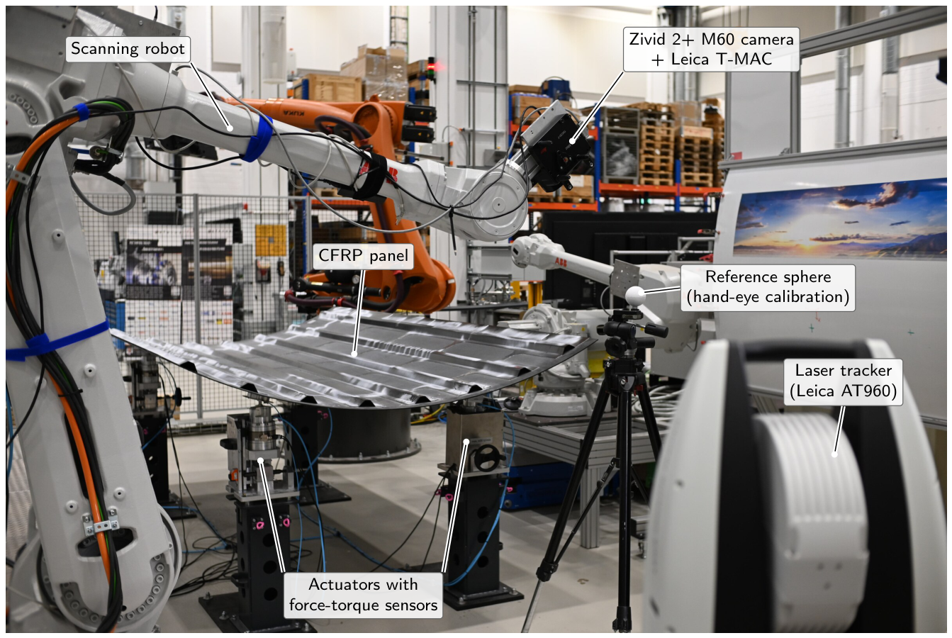
Figure 2.
Overview of the workflow. Process A stitches the captures of each configuration with the calibration chain of Section 4.3. Process B simulates the nominal panel on the measured supports under gravity and the actuator lifts of the configuration. The hybrid pipeline registers, compares and transfers the residual to the nominal geometry. The three validations (dashed) test the FE model independently of the manufacturing deviation (1, 2) and the configuration independence of the result (3).
Figure 2.
Overview of the workflow. Process A stitches the captures of each configuration with the calibration chain of Section 4.3. Process B simulates the nominal panel on the measured supports under gravity and the actuator lifts of the configuration. The hybrid pipeline registers, compares and transfers the residual to the nominal geometry. The three validations (dashed) test the FE model independently of the manufacturing deviation (1, 2) and the configuration independence of the result (3).
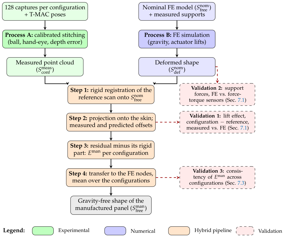
Figure 3.
The steps of the pipeline on the section mm (middle of a bay) of configuration A1, from the data of the campaign; medians in 10 mm bins along the arc s, gaps at the stringers and the margins. (a) Offset of the registered scan from the nominal skin along its normal and the offset predicted by the FE model (Steps 1–2); (b) their difference and its best-fitting rigid motion, fitted over the whole skin (Step 3); (c) at the skin nodes of the section in the eight configurations (grey) and their mean (Step 4); (d) nominal section and GFS, the nominal skin displaced by the mean along its normal (exaggerated 100 times).
Figure 3.
The steps of the pipeline on the section mm (middle of a bay) of configuration A1, from the data of the campaign; medians in 10 mm bins along the arc s, gaps at the stringers and the margins. (a) Offset of the registered scan from the nominal skin along its normal and the offset predicted by the FE model (Steps 1–2); (b) their difference and its best-fitting rigid motion, fitted over the whole skin (Step 3); (c) at the skin nodes of the section in the eight configurations (grey) and their mean (Step 4); (d) nominal section and GFS, the nominal skin displaced by the mean along its normal (exaggerated 100 times).
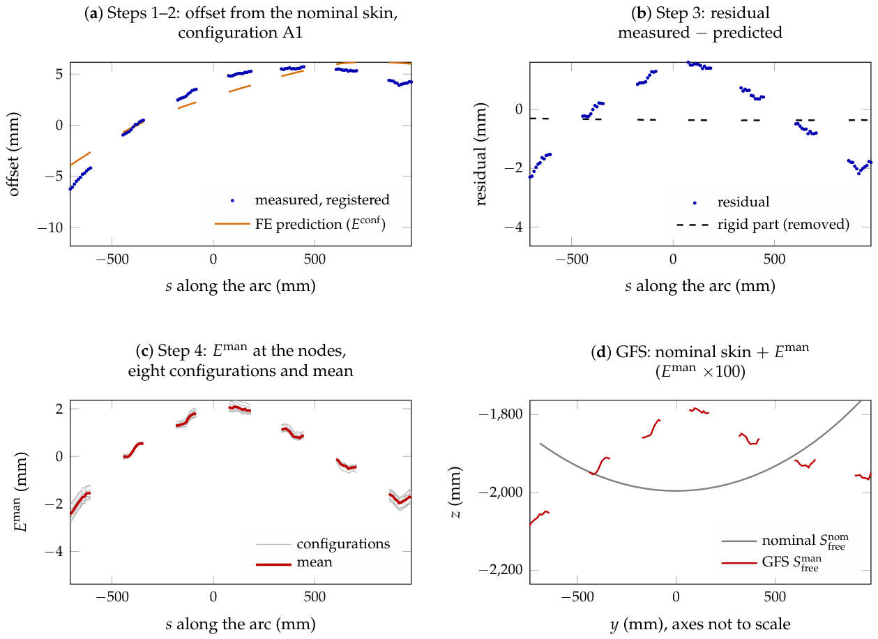
Figure 4.
Frames and transformations of the measurement chain. An arrow from frame b to frame a transforms coordinates from b to a. : T-MAC pose measured by the tracker for capture k; : hand-eye transformation from the reference-ball calibration (Section 4.3.1); : correction of the hand-eye rotation in the camera frame, estimated from the overlaps (dashed, Section 4.3.3). The depth error of the camera is corrected on the raw points, in the camera frame (Section 4.3.4).
Figure 4.
Frames and transformations of the measurement chain. An arrow from frame b to frame a transforms coordinates from b to a. : T-MAC pose measured by the tracker for capture k; : hand-eye transformation from the reference-ball calibration (Section 4.3.1); : correction of the hand-eye rotation in the camera frame, estimated from the overlaps (dashed, Section 4.3.3). The depth error of the camera is corrected on the raw points, in the camera frame (Section 4.3.4).

Figure 5.
Depth error of the camera along its optical axis (mm), joint fit with the hand-eye rotation on the overlaps of all eight runs. u: image width; v: image height, along the linear axis.
Figure 5.
Depth error of the camera along its optical axis (mm), joint fit with the hand-eye rotation on the overlaps of all eight runs. u: image width; v: image height, along the linear axis.
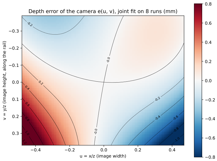
Figure 6.
Error budget of the stitching after each calibration step, eight runs (thin lines: individual runs; markers and values: mean of the runs). (a) Spread between the captures overlapping in a 5 mm cell; (b) median offset of the pairs of neighbouring stations and of neighbouring poses; (c) robust standard deviation ( median absolute deviation) of the pair distances d, and the point noise; (d) standard deviation of the pair-cell means of d, split into the part that repeats in every run and the part that changes from run to run.
Figure 6.
Error budget of the stitching after each calibration step, eight runs (thin lines: individual runs; markers and values: mean of the runs). (a) Spread between the captures overlapping in a 5 mm cell; (b) median offset of the pairs of neighbouring stations and of neighbouring poses; (c) robust standard deviation ( median absolute deviation) of the pair distances d, and the point noise; (d) standard deviation of the pair-cell means of d, split into the part that repeats in every run and the part that changes from run to run.
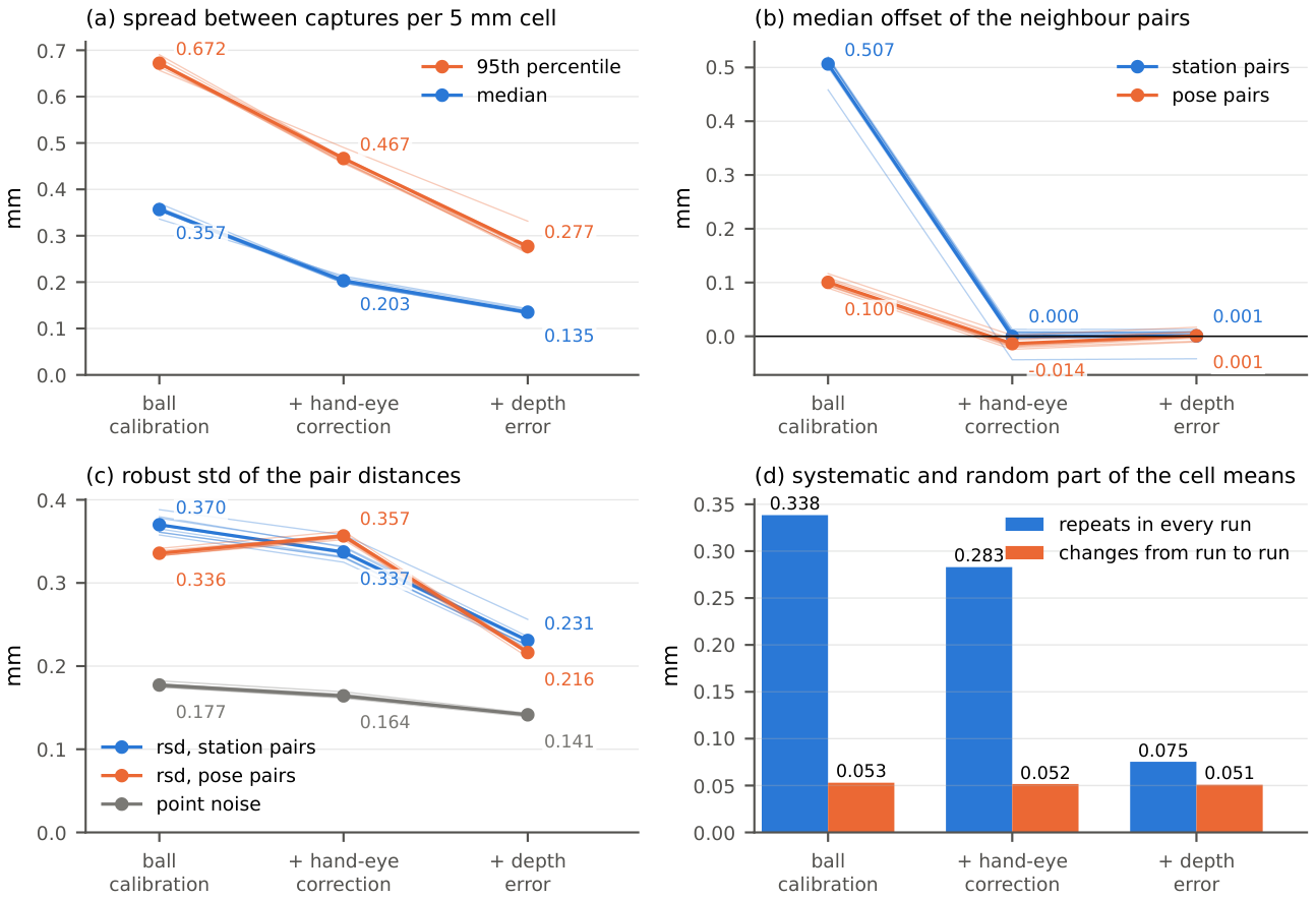
Figure 7.
Spread between captures per 5 mm cell against the number of captures overlapping the cell, before and after the hand-eye correction (eight runs; thick lines: median; bands: 25–75 % and 10–90 %; thin lines: median of each run). Bottom: number of cells per run.
Figure 7.
Spread between captures per 5 mm cell against the number of captures overlapping the cell, before and after the hand-eye correction (eight runs; thick lines: median; bands: 25–75 % and 10–90 %; thin lines: median of each run). Bottom: number of cells per run.
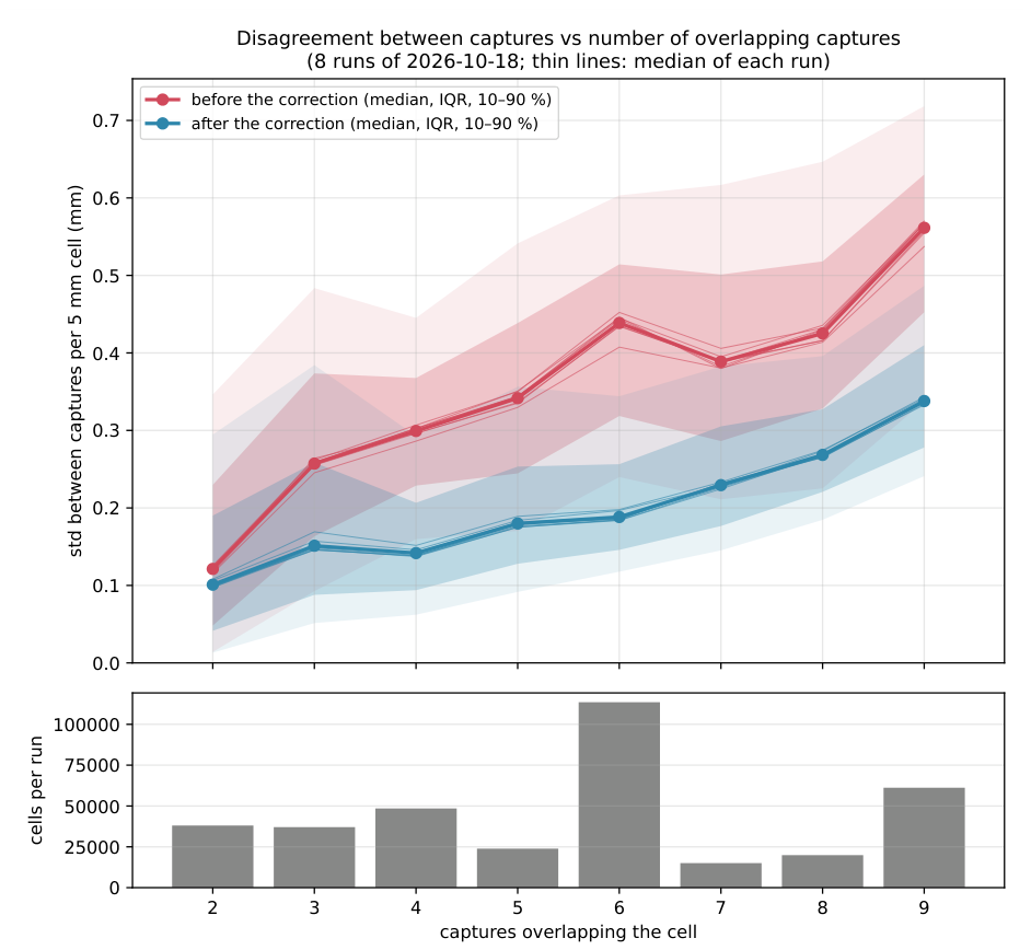
Figure 9.
Lift effect (configuration minus reference) with measured supports. (a–c) Configuration A1+A4: measured, predicted, and their difference on the unrolled skin (triangles: lifted actuators); (d) measured against predicted lift effect on the 20 mm cells of all seven lift cases; (e) rms of the difference per case, with the slope k and the correlation .
Figure 9.
Lift effect (configuration minus reference) with measured supports. (a–c) Configuration A1+A4: measured, predicted, and their difference on the unrolled skin (triangles: lifted actuators); (d) measured against predicted lift effect on the 20 mm cells of all seven lift cases; (e) rms of the difference per case, with the slope k and the correlation .
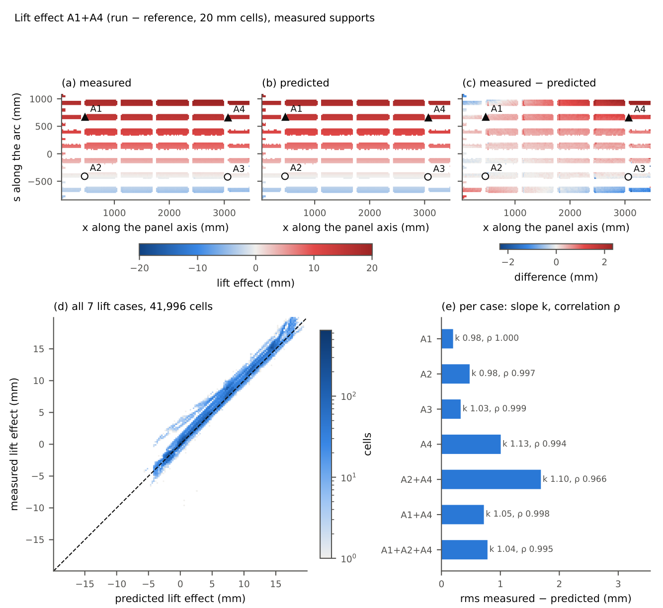
Figure 10.
Agreement of the clamped and the push-only support models per configuration. (a) Rms of the measured minus the predicted lift effect; (b) rms of the measured minus the predicted absolute offset from the nominal skin, after removal of the best-fitting rigid motion (registration).
Figure 10.
Agreement of the clamped and the push-only support models per configuration. (a) Rms of the measured minus the predicted lift effect; (b) rms of the measured minus the predicted absolute offset from the nominal skin, after removal of the best-fitting rigid motion (registration).
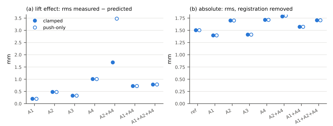
Figure 11.
Manufacturing deviation field on the unrolled skin (circles: actuators). (a) Mean over the eight configurations, positive towards the panel axis; (b) standard deviation of over the configurations per node. Grey: skin not evaluated, not seen by the scanner (dark) or within the margins at the stringers and the outline (light).
Figure 11.
Manufacturing deviation field on the unrolled skin (circles: actuators). (a) Mean over the eight configurations, positive towards the panel axis; (b) standard deviation of over the configurations per node. Grey: skin not evaluated, not seen by the scanner (dark) or within the margins at the stringers and the outline (light).
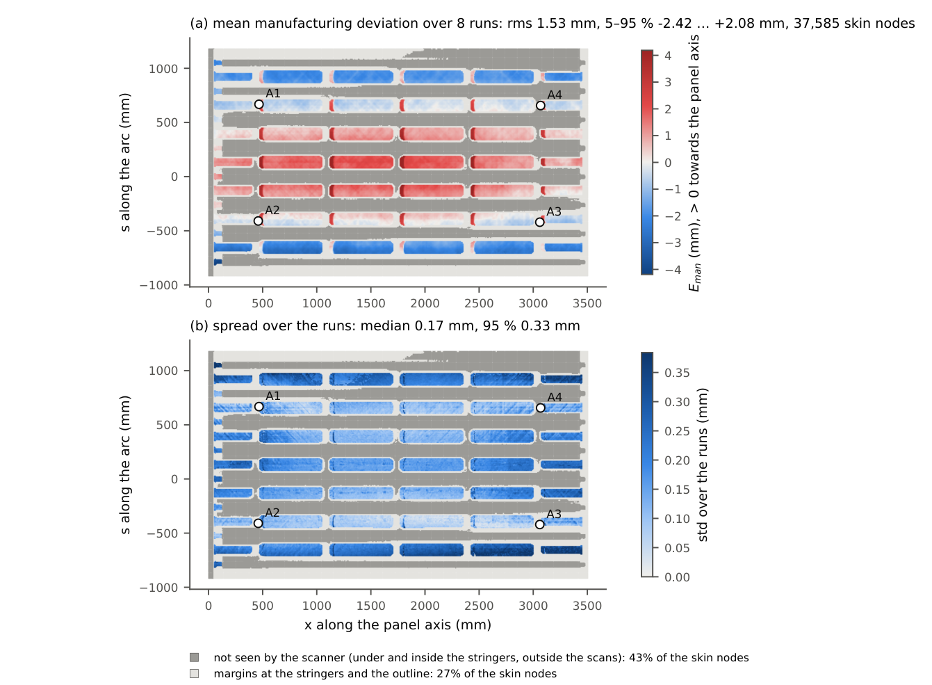
Figure 14.
Synthetic benchmark. A known deviation field is added to a truth FE shape at the real scan points of each configuration (G1, G2), with the measurement noise of a stitched point and a common rigid error (G3). The synthetic clouds pass through the unchanged pipeline, and the recovered is compared with . With truth = model, the comparison gives the error of the algorithm; with a truth that differs from the model (variants), it gives the part of a model error that the rigid registration passes into .
Figure 14.
Synthetic benchmark. A known deviation field is added to a truth FE shape at the real scan points of each configuration (G1, G2), with the measurement noise of a stitched point and a common rigid error (G3). The synthetic clouds pass through the unchanged pipeline, and the recovered is compared with . With truth = model, the comparison gives the error of the algorithm; with a truth that differs from the model (variants), it gives the part of a model error that the rigid registration passes into .
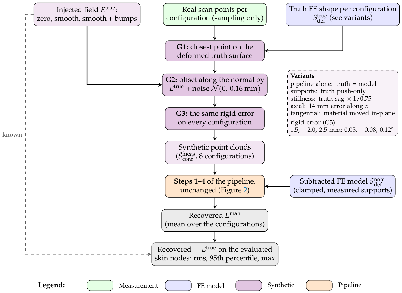
Figure 15.
Synthetic benchmark. (a) Error of the recovered mean for each benchmark (rms, 95th percentile, maximum) against the injected field of 1.42 mm rms; (b) injected field ; (c,d) recovered minus injected field for the pipeline alone and for a panel 25 % softer than the model.
Figure 15.
Synthetic benchmark. (a) Error of the recovered mean for each benchmark (rms, 95th percentile, maximum) against the injected field of 1.42 mm rms; (b) injected field ; (c,d) recovered minus injected field for the pipeline alone and for a panel 25 % softer than the model.
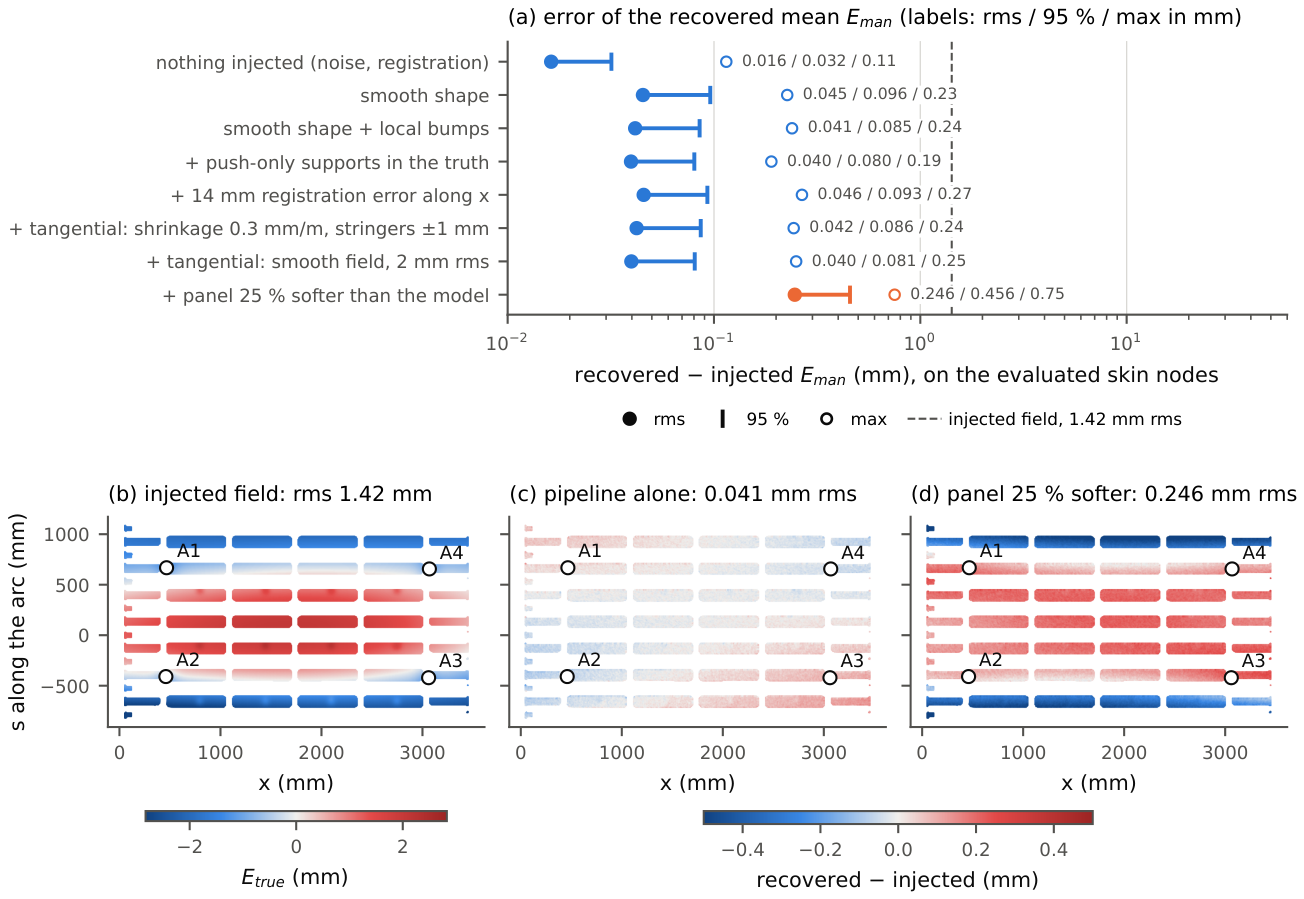
Figure 16.
Uncertainty sources of the workflow. Under or over each cause: how it enters the manufacturing deviation ; on each rib: its size where it was quantified (Section 4.4, Section 7.1 and Section 7.3).
Figure 16.
Uncertainty sources of the workflow. Under or over each cause: how it enters the manufacturing deviation ; on each rib: its size where it was quantified (Section 4.4, Section 7.1 and Section 7.3).
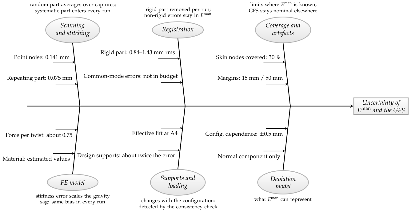

Table 1.
Classification of reviewed approaches by inspection strategy, fixture constraint, and material assumption.
Table 1.
Classification of reviewed approaches by inspection strategy, fixture constraint, and material assumption.
| Reference | Strategy | Fixture | Material | Application |
|---|---|---|---|---|
| Fixtureless geometric methods | ||||
| Radvar-Esfahlan & Tahan [19,20] | Geometric (GNIF) | None | Not required | Simulated parts |
| Sabri et al. [21,22] | FE-assisted | None | Isotropic | Sheet metal |
| Sattarpanah K. et al. [23,24] | FE-assisted | None | Isotropic | Aerospace panels |
| Babanezhad et al. [25] | Geometric + FE | None | Isotropic | Sheet metal |
| Measurement combined with FE simulation | ||||
| Lartigue et al. [26] | Meas. + FE | Non-overconstr. | Isotropic | Flexible parts |
| Thiébaut et al. [8] | Meas. + FE | Non-overconstr. | Isotropic | Flexible parts |
| Gringoz et al. [27] | Meas. + FE | Multi-point | Isotropic | Composite nacelle |
| Lindau et al. [28] | Meas. + FE | 3-point (non-OC) | Isotropic | Auto. sheet metal |
| Tuominen [29] | Virtual clamp | Non-overconstr. | Isotropic | Auto. welded assy. |
| Claus et al. [18] | Meas. + FE | Non-OC (required) | Isotropic | Sheet metal |
| Morse & Grohol [9] | Meas. + FE | Multi-point | Isotropic | Auto. fender |
| Reduced-order and surrogate methods | ||||
| Maltauro et al. [31] | Influence coeff. | Simple support | Isotropic | Sheet metal |
| Sensor-driven shape reconstruction | ||||
| Oboe et al. [32] | iFEM | N/A | Not required | Helicopter fuselage |
| Present work | Meas. + FE | Overconstr. | Anisotropic | CFRP fuselage panel |
Table 2.
Design of experiments: lift of each actuator relative to the reference configuration (mm).
| Configuration | A1 | A2 | A3 | A4 |
|---|---|---|---|---|
| Reference | 0 | 0 | 0 | 0 |
| A1 | 15 | 0 | 0 | 0 |
| A2 | 0 | 15 | 0 | 0 |
| A3 | 0 | 0 | 15 | 0 |
| A4 | 0 | 0 | 0 | 15 |
| A2+A4 | 0 | 15 | 0 | 15 |
| A1+A4 | 15 | 0 | 0 | 15 |
| A1+A2+A4 | 15 | 15 | 0 | 15 |
Table 3.
Uncertainty of a point of one capture after the calibration chain (1, mm, normal to the surface unless stated). Correction: Monte Carlo with 100 draws on the reference run; median over all points.
Table 3.
Uncertainty of a point of one capture after the calibration chain (1, mm, normal to the surface unless stated). Correction: Monte Carlo with 100 draws on the reference run; median over all points.
| Contribution | Type | Value |
|---|---|---|
| Point noise | random, per point | 0.141 |
| Cell part, changing from run to run | random, per capture | 0.036 |
| Cell part, repeating | systematic, not corrected | 0.053 |
| Correction, shape (rigid motion removed) | systematic, same in a run | 0.016 |
| Correction, shape, lateral to the surface | systematic, same in a run | 0.043 |
| Combined, one capture, shape | 0.156 |
Table 4.
Ply material of the FE model (estimates of the model supplier).
| Property | Value |
|---|---|
| Longitudinal Young’s modulus | 135 GPa |
| Transverse Young’s modulus | 10 GPa |
| Shear moduli | 5 GPa |
| Poisson’s ratio | 0.30 |
| Density | 1600 kg/m3 |
Table 5.
Sensitivity of the FE prediction to the idealisation of the supports, per configuration: change of the normal displacement of the skin without its best-fitting rigid motion (rms and maximum, mm) and largest change of a vertical support force (, N) between two simulations that differ only in the contact law (clamped or push-only heads), the in-plane lock of A3 (locked or free) or the geometric nonlinearity (on or off, with clamped or push-only heads; computed with A3 locked, which changes the prediction by at most 0.02 mm, see the columns of the in-plane lock).
Table 5.
Sensitivity of the FE prediction to the idealisation of the supports, per configuration: change of the normal displacement of the skin without its best-fitting rigid motion (rms and maximum, mm) and largest change of a vertical support force (, N) between two simulations that differ only in the contact law (clamped or push-only heads), the in-plane lock of A3 (locked or free) or the geometric nonlinearity (on or off, with clamped or push-only heads; computed with A3 locked, which changes the prediction by at most 0.02 mm, see the columns of the in-plane lock).
| Geometric nonlinearity | ||||||||||||
|---|---|---|---|---|---|---|---|---|---|---|---|---|
| Contact law | In-plane lock of A3 | Clamped | Push-only | |||||||||
| Configuration | rms | max | rms | max | rms | max | rms | max | ||||
| Reference | 0.00 | 0.00 | 0.0 | 0.00 | 0.00 | 0.0 | 0.01 | 0.02 | 0.0 | 0.01 | 0.02 | 0.0 |
| A1 | 0.01 | 0.02 | 0.3 | 0.01 | 0.01 | 0.2 | 0.03 | 0.11 | 1.2 | 0.03 | 0.11 | 1.2 |
| A2 | 0.01 | 0.02 | 0.3 | 0.01 | 0.02 | 0.1 | 0.03 | 0.10 | 1.4 | 0.03 | 0.10 | 1.4 |
| A3 | 0.01 | 0.02 | 0.3 | 0.01 | 0.02 | 0.2 | 0.03 | 0.11 | 1.2 | 0.03 | 0.11 | 1.2 |
| A4 | 0.01 | 0.02 | 0.3 | 0.00 | 0.01 | 0.1 | 0.03 | 0.10 | 1.3 | 0.03 | 0.10 | 1.3 |
| A2+A4 | 1.38 | 3.05 | 62.0 | 0.01 | 0.02 | 0.3 | 0.10 | 0.34 | 2.4 | 0.07 | 0.21 | 0.1 |
| A1+A4 | 0.00 | 0.00 | 0.0 | 0.00 | 0.00 | 0.0 | 0.02 | 0.03 | 0.1 | 0.02 | 0.03 | 0.1 |
| A1+A2+A4 | 0.01 | 0.02 | 0.3 | 0.00 | 0.01 | 0.1 | 0.03 | 0.10 | 1.4 | 0.03 | 0.10 | 1.4 |
Table 6.
Change of the support force from the reference configuration (N, positive: more load), measured by the force-torque sensors (axial force ) and predicted (vertical force) by the FE model with measured, clamped supports, and the ratio of measured to predicted.
Table 6.
Change of the support force from the reference configuration (N, positive: more load), measured by the force-torque sensors (axial force ) and predicted (vertical force) by the FE model with measured, clamped supports, and the ratio of measured to predicted.
| Configuration | Measured/FE | ||||
|---|---|---|---|---|---|
| A1, measured | 0.74 | ||||
| A1, FE | |||||
| A2, measured | 0.69 | ||||
| A2, FE | |||||
| A3, measured | 0.75 | ||||
| A3, FE | |||||
| A4, measured | 0.71 | ||||
| A4, FE | |||||
| A2+A4, measured | 0.48 | ||||
| A2+A4, FE | |||||
| A1+A4, measured | – | ||||
| A1+A4, FE | |||||
| A1+A2+A4, measured | 0.34 | ||||
| A1+A2+A4, FE |
Table 7.
Quantified uncertainty contributions.
| Contribution | Value |
|---|---|
| Stitching: spread between overlapping captures, after correction (median per 5 mm cell) | 0.13 mm |
| Stitching: part repeating in every run / changing from run to run | 0.08 mm / 0.05 mm |
| Shape of a single capture, combined standard uncertainty (Monte Carlo) | 0.16 mm |
| Registration: rigid part of the residual, removed per run | 0.84–1.43 mm rms |
| : spread over the configurations (median / 95th percentile per node) | 0.17 mm / 0.33 mm |
| : remaining configuration dependence (arc curvature) | about mm |
| FE model: lift effect, measured supports, single lifts (rms difference) | 0.20–1.0 mm |
| FE model: measured / predicted force per unit twist | about 0.75 |
| FE model: bias of if uniformly 25 % too stiff (rms / 95th percentile) | 0.25 mm / 0.46 mm |
| Combined standard uncertainty of the GFS offset per node (median / 95th percentile) | 0.24 mm / 0.52 mm |
| without the stiffness of the model | 0.14 mm / 0.24 mm |
| Expanded uncertainty U (, median / 95th percentile) | 0.49 mm / 1.03 mm |
Disclaimer/Publisher’s Note: The statements, opinions and data contained in all publications are solely those of the individual author(s) and contributor(s) and not of MDPI and/or the editor(s). MDPI and/or the editor(s) disclaim responsibility for any injury to people or property resulting from any ideas, methods, instructions or products referred to in the content. |
© 2026 by the authors. Licensee MDPI, Basel, Switzerland. This article is an open access article distributed under the terms and conditions of the Creative Commons Attribution (CC BY) license (http://creativecommons.org/licenses/by/4.0/).
Copyright: This open access article is published under a Creative Commons CC BY 4.0 license, which permit the free download, distribution, and reuse, provided that the author and preprint are cited in any reuse.