

Submitted:
12 October 2026
Posted:
13 October 2026
You are already at the latest version
Abstract
Accurate State of Health (SOH) estimation is essential for the safe and reliable operation of lithium-ion batteries (LIBs), yet most electrochemical impedance spectroscopy (EIS)-based approaches fix a single equivalent circuit model (ECM) topology and measurement state without testing whether that choice is actually the most degradation-sensitive one, and rarely cross-check circuit-based findings against an independent, model-agnostic representation of the same impedance data. This study addresses both gaps through a physics-constrained framework applied to four commercial Li-ion cells cycled to end of life, with EIS spectra acquired at nine states in a cycle. Six ECM topologies (1R to 2RCPEW) were fitted at each state, and Pearson Correlation Coefficient was used to jointly rank topology–state combinations by their sensitivity to capacity fade. The best-ranked ECM parameters were then used as input to a left-to-right Hidden Markov Model (HMM) to segment battery ageing into ordered latent degradation regimes, with results compared against an HMM applied to DINOv2 embeddings of Nyquist and DRT plots. Finally, Gaussian Process Regression (GPR) was used to estimate SOH with and without the HMM-derived regime label as an auxiliary feature. Results show that State V (reached after a post-charge rest) yields the highest degradation sensitivity for most ECMs, with ohmic and charge-transfer resistances as the dominant health factors. Adding the latent regime feature improved SOH prediction for the 1RC and 1RCPE models (MAE reduced by up to 46.5%) but degraded uncertainty calibration for the 2RC model, indicating that the value of latent degradation information depends on how much temporal structure the underlying ECM already captures.
Keywords:
Li-ion batteries
; EIS
; SOH estimation
; vision transformer
; equivalent circuit models
; Hidden Markov Model
1. Introduction
Li-ion batteries characteristics such as high energy density and long cycle life, introduce safety challenges: as energy density increases, the risk of high-impact thermal runaway can grow, and faults such as short circuits, mechanical abuse, or manufacturing defects can result in fire or explosion [1]. Beyond immediate safety hazards, battery degradation (commonly due to cycling and calendar ageing) can compromise system performance and reliability, potentially leading to severe incidents such as traffic accidents or large-scale power outages. To mitigate these risks and prevent those scenarios, accurate diagnosis of the battery State of Health (SOH) is essential.
Estimating the SOH and operational lifespan of electric vehicle (EV) batteries, depends on reliable algorithms, and still represents a complex challenge for a wide range of stakeholders [2]. Such estimates are critical for ensuring safety, planning maintenance, optimizing performance, reducing warranty and replacement costs, and informing long-term design decisions. Consequently, the precise characterization and prediction of lithium-ion battery (LIB) degradation have become fundamental requirements for advancing battery design, management, and overall system operation [2].
Existing performance estimation strategies fall into three main categories: model-based, data-driven, and hybrid approaches. Model-based techniques rely on mathematically representing either the internal electrochemical processes or the observable external behavior of the battery [3,4,5]. Within this class, equivalent circuit models (ECMs) are particularly advantageous, offering a practical compromise between physical fidelity and computational efficiency. ECMs capture key battery dynamics with significantly reduced complexity compared to full electrochemical models, making them well-suited for real-time battery management system (BMS) implementation.
Data-driven SOH estimation methods rely exclusively on operational measurements to train predictive models. Even without detailed inner cell electrochemical analysis, this approach offers strong adaptability and the ability to capture nonlinear battery behaviors [3,6,7]. The majority of published studies adopting this methodology rely on data collected under controlled laboratory conditions [8,9], physics-based simulations [10,11], or curated public datasets such as the NASA Ames [12], CALCE [13], Stanford/MIT Fast-Charging [14], and HNEI benchmarks [15,16]. There are numerous models implemented to capture the degradation signature in cell performance, ranging from classical models, such as Random Forest (RF) [17] and Gaussian Process Regression (GPR) [18], to Neural Network-based models, such as Long Short-Term Memory (LSTM) [19], Gated Recurrent Unit (GRU) [6] and Convolutional Neural Network [20], to more advanced models such as Transformers [21]. However, since the BMS reliability is strictly connected with uncertainty calibration of the adopted model, GPR, with built-in probability estimation capability, is commonly deemed more suitable for reliable SOH estimation [3,18].
Hybrid estimation techniques further enhance accuracy and robustness by integrating the physical interpretability and stability of model-based methods with the flexibility and pattern-recognition capabilities of data-driven models [22]. This combination enables more reliable and generalizable SOH predictions across diverse usage conditions.
As LIBs age through repeated charge–discharge cycling, their capacity diminishes, resulting in reduced available energy and observable shifts in the voltage profile. Effective SOH estimation therefore depends on identifying relevant health factors (HFs) that can adequately capture these degradation-related changes. Electrochemical impedance spectroscopy (EIS) is one of the most powerful techniques for monitoring internal electrochemical processes in LIBs. EIS is typically visualized using Nyquist plots, where the real and imaginary components of impedance are plotted. Akram et al. [23] proposed a data-driven framework for SOH estimation by combining EIS with Distribution of Relaxation Times (DRT) to resolve overlapping electrochemical processes. Specifically, the authors extracted four key parameters as HFs from the charge transfer peak: area, height, Full Width at Half Maximum (FWHM) and center relaxation time. These features were then utilized to train a LSTM model, which captured the long-term temporal dependencies of battery ageing, with an estimation accuracy given by a Mean Absolute Error (MAE) of 1.28%. In another study, Thomas et al. [24] developed a Salient Frequency Extraction (SFE) algorithm to identify the frequencies in EIS data that exhibited the strongest relationship with battery degradation, particularly within the charge transfer region. By focusing only on these high-correlation data points, the study demonstrated that it is possible to maintain high accuracy in SOH and capacity prediction while reducing data acquisition time.
Fitting EIS data to an ECM provided a means of mapping spectral features to battery kinetic processes [25]. It was shown that, compared with other characterization methods, EIS offers several advantages: it provides access to kinetic parameters, it is non-destructive, and suitable for in situ or operando monitoring of battery states [26]. A range of ECMs has been proposed to represent the electrical behavior of LIBs, with increasing complexity typically achieved by adding Resistor–Capacitor (RC) branches [27,28]. The 1RC model consists of an ohmic resistance and one parallel RC branch, capturing the instantaneous voltage drop and one dominant transient polarization process. A 2RC model adds a second RC branch with a different time constant, enabling the representation of multiple dynamic processes occurring over different time scales, while higher-order ECMs can include additional RC branches for greater modeling flexibility [27,28]. In EIS-based ECM fitting, the resistances and capacitances of these branches are estimated so that the model-predicted impedance matches the measured impedance across the investigated frequency range. Increasing the number of RC branches can improve the representation of complex electrochemical dynamics but also increases the number of parameters and the risk of overfitting. Consequently, the choice of ECM order involves a trade-off between model fidelity, parameter identifiability, and computational complexity.
Ibrahim et al. [29], proposed a passive fast Fourier transform (FFT)-based EIS framework for real-time SOH estimation of lithium-ion capacitors (LICs). The method extracted ECM parameters directly from operational current and voltage data without requiring external excitation, enabling real-time impedance analysis and accurate SOH prediction, with a reported MAE of 2.23%. In another study [30], second-life LIBs were cycled under various laboratory conditions to investigate battery degradation. The temporal dynamics of EIS measurements were analyzed, and a computationally efficient machine learning model was developed for SOH estimation. In addition, a fractional-order ECM was employed to characterize battery degradation mechanisms, enabling the analysis of three primary degradation modes: capacity loss (CL), loss of lithium inventory (LLI), and loss of active material (LAM).
Most existing EIS-based SOH studies select a single ECM topology and measurement state (i.e., a fixed point within the charge–discharge cycle, such as fully charged or mid-discharge), without systematically evaluating which topology–state combination is most sensitive to degradation. Furthermore, to our knowledge, relatively small number of studies [31] has integrated ECM-derived features with image-based representations, such as Nyquist plots and DRT maps, for unsupervised degradation-state discovery.
This is a meaningful limitation for two reasons. First, different ECM topologies emphasize different electrochemical processes; a single RC pair mainly captures fast charge-transfer kinetics, while additional RC branches or Warburg elements are needed to resolve slower diffusion-related effects [28]. Therefore, the SOH-sensitivity of a topology’s fitted parameters is not guaranteed to be uniform across the different points of a charge–discharge cycle. A model that performs well when fit to spectra taken at one operating state may perform poorly at another, simply because the process it is best equipped to represent is not the dominant one occurring at that state. Fixing both the topology and the state without first testing this interaction therefore risks selecting a HF that is degradation-sensitive by convention rather than by evidence. Second, relying solely on hand-picked circuit models leaves no independent check on whether the resulting latent degradation regimes are physically meaningful: an image-based, model-agnostic representation of the same impedance data (e.g., via Nyquist or DRT plots) offers a complementary route to degradation-state discovery that does not depend on the correctness of any single circuit assumption.
The objective of this study is therefore not simply to improve SOH prediction accuracy by adding a machine-learning model to EIS measurements. Instead, the central question is how the representation and measurement condition of EIS influence the degradation information available to a health estimator. The paper investigates this question at three levels. First, it systematically evaluates the interaction between ECM topology and measurement state to identify combinations whose fitted parameters are most sensitive to capacity degradation. Second, rather than assuming that degradation evolves as a single smooth regression trajectory, the paper investigates whether these degradation-sensitive features can be used to segment battery ageing into ordered latent degradation regimes. Third, it tests whether this regime information provides predictive information beyond the ECM parameters themselves when estimating SOH with a probabilistic regression model. Importantly, the framework is also evaluated against an image-based, model-agnostic representation of the same EIS information using Nyquist and DRT plots. This comparison is intended not to assume that a more complex representation is necessarily superior, but to determine whether degradation information identified from a circuit-based representation is also reflected in an independent representation of the impedance response.
2. Methods
The physics-constrained methodology proposed in this study is based on open-access EIS data [32], derived from commercially available 45 mAh Li-ion coin cells (LiCoO₂/graphite) subjected to continuous charge–discharge cycling under controlled temperatures. Cells no. 4, 6, 7 and 8 were selected from the dataset, as these were characterized with a clear capacity-fade pattern and EIS records across all measurement states for the full cycle life. After 30 formation cycles at 25 °C, each of the four selected cells was charged at 1C (45 mA) to 4.2 V using a CC–CV protocol and discharged at 2C (90 mA) to 3.0 V at 25 °C; capacity was measured every odd cycle. EIS spectra were acquired during every even cycle at nine states spanning the CC–CV charge and discharge process, using a 5 mA excitation amplitude over 0.02 Hz–20 kHz. The above nine states (denoted as I-IX) were reported as follows [32]: I: Before charging; II: Start charging; III: After 20 minutes charging; IV: After charging and before resting; V: After a 15 minute rest; VI: Start discharging; VII: After 10 minutes discharging; VIII: After discharging and before resting; IX: After 15 minutes rest.
As the battery ages, its capacity declines due to several internal mechanisms, and this trend can be adopted as a key indicator of approaching the End of Life of the cell. In the present study, SOH has been adopted as the output of the predictive model and can be defined by the following ratio:
where Q0 is the nominal capacity of the cell and Qn is the maximum discharge capacity of the cell after n cycles.
2.1. Equivalent Circuit Model
The health-factor extraction process begins by using a Python impedance library to fit measured EIS spectra to several ECMs, allowing key parameters to be optimized through nonlinear least-squares technique. For each cycle and state in the dataset, the fitting procedure took the complex impedance data across frequencies and determined the set of ECM parameters that best reproduced the impedance curve, yielding a consistent representation of the battery internal state. These extracted resistances served as quantitative HFs, capturing changes in charge-transfer resistance, diffusion behavior, and overall impedance growth as the battery aged. A range of models were studied, namely 1R, 1RC, 1RCPE, 2RC, 2RCPE and 2RCPEW (Figure 1). The formulations for ECMs are reported in [27,28,33]. Table 1 summarizes the structure and physical interpretation of each topology.
To check how closely each factor related to SOH, the Pearson Correlation Coefficient (PCC) was used:
where xi and yi respectively represent the i-th sample value of variables x and y, and and respectively represent the sample means of variables x and y.
As mentioned, although a given ECM topology can in principle be fit to impedance spectra recorded at any operating state, the degradation-sensitivity of its fitted parameters is not necessarily uniform across states: each state emphasizes different electrochemical processes (e.g., charge-transfer-dominated behavior shortly after starting to charge or discharge, versus diffusion/relaxation-dominated behavior after a rest period), which a given circuit topology may capture with different fidelity. The model and state were therefore screened jointly, rather than assuming any single topology would perform in a constant way irrespective of measurement state. In order to identify which combination of ECM topology and battery operating state most strongly reflected cells capacity degradation, the PCC was computed between each fitted ECM parameter and the SOH across all battery cells, states, and candidate models, and then these correlations were aggregated and averaged to rank topology–state combinations. For each combination topology-state, the parameters exhibiting the highest mean absolute PCC with SOH was assessed. For a given model topology m and state s, the aggregated PCC was computed as:
where θc,p,m,s denotes the fitted value of parameter p of topology m at state s for cell c, and the correlation is computed across cycles on the same cell. Topology-state combinations were ranked by , and for each group the individual parameter with the highest mean |PCC|across cells was reported as that group’s best parameter. The topology–state combinations were then ranked according to their overall mean absolute PCC, and the highest-ranked combinations were selected for the subsequent stage of the study, clustering and SOH estimation.
2.2. Clustering via Hidden Markov Modeling (HMM)
After converting the measured impedance spectrum into a small number of physically interpretable parameters by ECM, the HMM (which will be discussed in more detail later) was then used for classifying the evolution of these parameters over successive cycles to identify latent degradation regimes. For comparison, a pre-trained unsupervised Visual Transformer (ViT) was used to convert Nyquist and DRT plots (generated from EIS data) into numerical feature vectors (called embeddings), allowing latent degradation patterns to be identified from the visual evolution of the impedance response.
Rather than treating capacity fade as a single continuous regression target, this study adopted an unsupervised sequential clustering step for two reasons. First, LIB degradation is widely reported [14,34] to progress through distinct phases (an early break-in period, a near-linear ageing phase, and an accelerated end-of-life phase) driven by different combinations of degradation mechanisms whose relative contribution shifts over the cell’s life. Fitting a single global regression to the ECM parameters implicitly assumes a stationary relationship between the HFs and SOH throughout life, an assumption that may break down if the dominant mechanism itself changes. Clustering cycles into latent regimes provides an explicit, data-driven representation of these ageing phases without requiring prior knowledge of when transitions occur. Second, because the regime label is intended as an auxiliary input to the downstream GPR model rather than a standalone diagnostic, its purpose is to supply the regressor with information about a cell’s position along its ageing trajectory. An HMM is well suited to this role because, unlike static clustering methods (e.g., k-means), it explicitly models the temporal ordering of observations and can be constrained to be monotonic consistent with irreversible battery ageing.
A Hidden Markov Model [35] is a probabilistic model that clusters sequential data by assuming that each observation can be associated with an underlying, unobserved (hidden) regime or cluster. It also models how likely the data is to transition from one regime to another over time, making it useful for clustering sequential observations, such as battery degradation. Therefore, HMM was used as a temporal segmentation method, assuming that each cycle belongs to one of several latent regimes to estimate the most likely sequence of regimes from the observed EIS-derived features (either ECM parameters or Nyquist/DRT embeddings).
A left-to-right structure was used to reflect the assumption that battery degradation progresses in one direction over time. Therefore, a battery could remain in its current state or move to the next, more degraded state, but it could not return to a previous state. To enforce this behavior, each state had a high probability of remaining in the same state, while the final state was set as an absorbing state with a self-transition probability of 1.0 (it means whatever in this state does not transit to another). All sequences were initialized in state 0, representing the least-degraded condition. The transition probabilities and initial state probabilities were fixed throughout the training process. The model instead learned the characteristics of each degradation state, represented by the mean and covariance of the observed features. In practical terms, the model converts a continuously changing degradation trajectory into a sequence such as early-life, intermediate-ageing, and late-life regimes, which should be interpreted as statistically defined degradation segments rather than as direct measurements of individual physical degradation mechanisms.
Since the number of hidden states (degradation clusters) is unknown as priori, HMMs were fitted for each candidate value of n states within a specified range (2 to 14). For each candidate, the model’s log-likelihood was used to compute the Bayesian Information Criterion (BIC) [36], which penalizes model complexity to avoid selecting an excessive number of states purely because it improves fitting:
where log L is the model log-likelihood, n is the number of observations, and k is the number of free parameters. The BIC penalizes model complexity to avoid overfitting to an excessive number of states. The number of states minimizing BIC across all candidates was selected as the optimal model order.
BIC= −2∙logL + k∙logn,
The cycle-level features used as inputs to HMM were divided into two candidate sets: ECM-based and image-based features. The ECM-based features consisted of the parameters of the previously selected ECM at the chosen operating state, according to the procedure described in Section 2.1. The image-based features comprised embeddings extracted from Nyquist and DRT plots using DINOv2 (a ViT model) applied directly to the rendered plot images rather than to the raw numerical impedance spectra. The topology-state ranking was then used to select the ECM parameters for the first feature set, while the DINOv2-based embeddings were used for the second feature set, as described in the following section.
Nyquist plots represent EIS data by plotting the negative imaginary part of impedance against the real part across the measured frequency range, typically producing one or more semicircular arcs whose diameters and shapes reflect process parameters such as ohmic resistance, charge-transfer resistance, and diffusion. On the other hand, the DRT plot transforms the impedance response by decomposing it into contributions from processes with different characteristic relaxation times, producing peaks that correspond to these processes. This allows overlapping electrochemical processes to be separated and identified based on the location and magnitude of their peaks. In this study, DRT plots were obtained based on a method defined by Huang et al. [37].
Two set of images (Nyquist and DRT) based on EIS data of Zhang et al. [32] spanning the full cycle life of each cell (8,148 plots), and providing a visual, model-agnostic encoding of impedance evolution as a function of degradation, were generated (two examples are illustrated in Figure 2). They were preprocessed following standard normalization (resize, center-crop, followed by channel-wise normalization), and then passed through a pre-trained self-supervised vision transformer, DINOv2 (ViT-B/14), to extract a high dimension fixed-length embedding vector (with 768 length) per image.
DINOv2 [38] was trained purely from the structure and consistency of the images themselves, at very large scale (over 140 million curated natural images). This training paradigm produced embeddings that generalized well across domains substantially different from the model original training distribution. More detail on architecture of this model can be found in [38]. Since battery degradation is gradual, change in impedance-response geometry is continuous (e.g., growing semicircle diameter, shifting relaxation-time peaks), a feature extractor sensitive to subtle shape and texture variations is required. The patch-based self-attention mechanism of the ViT backbone is well suited to capturing exactly this kind of localized geometric changes.
Due to the fact that each DINOv2 embeddings contains high dimensional feature set, Principal Component Analysis (PCA) [39] was used to reduce the embedding into a smaller set of variables while retaining the dominant variation in the image representation. PCA is a dimensionality-reduction method that transforms the input features into new features set called principal components. PCA forms linear combinations of the original features and identifies directions that capture the largest variation in the data. The first principal component captures most of the variance, followed by subsequent components, allowing the dimensionality of the data to be reduced while retaining its main patterns. This reduction is necessary because the subsequent HMM estimates a covariance matrix for each latent regime, which becomes increasingly difficult and unstable as the number of input dimensions grows. To evaluate the sensitivity of downstream clustering to embedding dimensionality, two set of PCAs were tested: a 16-component and a 32-component. This dimensionality reduction step both mitigates the dimensionality issue for the subsequent HMM and suppresses embedding noise unrelated to degradation-relevant visual variation.
2.3. Predictive Model
The benefit of using the latent regime labels obtained from the HMM clustering procedure described above, as an auxiliary input for probabilistic SOH estimation, was subsequently assessed. To evaluate the added value of the degradation-state feature (Cluster) derived from the HMM clustering procedure, SOH was estimated by adopting GPR model under two feature sets: one including the HMM-derived regime label and one excluding it. GPR is a probabilistic, non-parametric regression method that models data by defining a distribution over functions rather than assuming a predetermined functional form. Its ability to generalize well under limited data conditions and avoid overfitting makes GPR an effective and widely adopted technique [18,40,41]. In the present study, usage of GPR is extended from SOH point estimate to quantify uncertainty of the model. This distinction is important for battery management because an SOH estimate accompanied by a calibrated uncertainty range can indicate when the model is confident in its diagnosis and when the prediction should be treated with caution.
Data from two battery cells (25C04 and 25C06) were used as the training set. A separate cell (25C07) was retained as a validation set, and another cell (25C08) was set as a test set. The validation cell was used exclusively for hyperparameter selection (e.g., choosing the number of HMM states via BIC, the PCA dimensionality), while the test cell was reserved exclusively for final, unbiased performance reporting and played no role in any training. This cell-wise splitting strategy ensures that the model is evaluated on entirely unseen battery units, providing a more realistic assessment of generalization than a random split within a single cell’s data.
2.4. Performance Analysis
For evaluating regression performance, a range of common metrics are available, including:
- the mean absolute error (MAE)
- the Root Mean Square Error (RMSE), the Standard deviation of residual errors describing the spread of prediction errors
- the Mean Prediction Interval Width (MPIW), i.e. the average width of the 95% prediction interval, reflecting the model’s confidence (sharpness)
- the Prediction Interval Coverage Probability (PICP), the percentage of true test-set SOH values falling within the predicted 95% interval, reflecting calibration reliability.
These metrics can be calculated as follows:
where yi, and are the actual and the predicted values of the output, respectively, and n is the number of observations;
where Li and Ui are the lower (2.5th percentile) and upper (97.5th percentile) bounds of the prediction interval for cycle i, and I(-) is the indicator function that takes value 1 if the condition in its argument is satisfied and 0 otherwise. A smaller MPIW indicates more precise predictions, but excessively narrow intervals may reduce coverage.
3. Results
3.1. Topology-State Ranking
Based on the ranking results in Table 2, State V consistently emerged as the most informative operating point for extracting degradation-sensitive EIS features across the majority of ECMs. Specifically, the 1RC, 1RCPE, 2RCPE, and 2RCPEW models all achieved their highest average PCC with SOH when parameters were extracted at State V. Two exceptions were observed: the 2RC model performed best at State I, and the single-parameter 1R model performed best at State VII, indicating that the optimal measurement state also depends on circuit complexity. Overall, these findings support the use of State V as the preferred operating point for subsequent feature extraction and SOH estimation, as it offers the highest degradation sensitivity across the majority of the evaluated ECMs. This finding carries a practical operative consequence: State V is reached after a 15-minute rest following full charge, meaning the most diagnostically informative measurement is not instantaneously available during active cycling. In a deployed BMS, this implies scheduling EIS acquisition during rest periods (e.g., overnight charging pauses). Notably, the top-ranked topology-state combination overall corresponds to the simplest RC-type model (1RC) rather than a higher-order one, indicating that additional RC branches do not necessarily increase degradation sensitivity and that a compact circuit can be sufficient for this purpose.
The results presented in Table 2 also identify the circuit parameter with the strongest average correlation to SOH for each ECM and operating state. A clear pattern emerges in which resistance-related parameters consistently dominate as the most informative health indicators. For the 1RC model, the ohmic resistance (R0) was identified as the best parameter across States V, IV, and IX, indicating that the increase in internal resistance provides a reliable measure of battery degradation within this model. On the other hand, for the 1RCPE model, the charge-transfer resistance (R1) was consistently selected as the most informative parameter in States I, IV, V, and IX, suggesting that degradation mechanisms associated with electrochemical charge transfer are more effectively captured when a constant phase element is included in the circuit representation. Similarly, the 2RC model achieved its highest correlation through R0 at State I, while the simpler 1R model also identified R0 at State VII as the dominant degradation-sensitive feature. Overall, a topology-dependent pattern can be observed: for the purely resistive-capacitive circuits (1R, 1RC, 2RC) the ohmic resistance (R0) is consistently the most degradation-sensitive parameter, whereas for the circuit incorporating a constant-phase element (1RCPE) the charge-transfer resistance (R1) becomes dominant, suggesting that the parameter exhibiting the strongest association with SOH depends on the ECM topology, with R0 dominating for the tested RC models and R1 dominating for the 1RCPE model.
3.2. Latent Degradation Clustering
Figure 3 compares the degradation-state trajectories recovered by the ECM-parameter-based HMM (namely for 1RC, 1RCPE, and 2RC with a fixed State V for comparison) against the image-embedding-based HMM applied to Nyquist and DRT plots (each reduced via PCA to 16 and 32 components), for each battery cell. The number of resolved states varies considerably across cells. For instance, cell 25C04 resolves into a comparatively smaller set of states (up to ~6) over its ~35-cycle life, while 25C06, with a longer cycle life (~250 cycles), is segmented into a higher set of states (up to ~14) by the ECM-based method.
Since the HMM-derived regime label is used as an auxiliary input feature to the GPR regression rather than as a standalone physical indicator, a higher number of labels simply carries more information for the regression to exploit, and the results in Table 3 will confirm this; i.e., clustering improved MAE and RMSE for both the 1RC and 1RCPE models.
Despite differing in total resolved state count, the different HMMs recognized a regime boundary (interpreted as the approximation onset of the degradation phase) at approximately the same cycle number, though the character of that agreement differs by cell. In 25C04 most methods showed a transition around cycle 22, around cycle 30 for 25C08, and around cycle 100 for 25C07, suggesting a fairly sharp, well-defined point near end-of-life for these cells. 25C06 shows a similar late-life convergence around cycle 170, but it is more gradual and spread across a wider span (148–198) rather than a single sharp point, indicating the transition unfolds over a longer stretch of cycles for this cell. Together, these patterns suggest that while a late-life, high-resistance-growth signature is consistently detectable across both ECM-based and image-based methods, its sharpness, timing, and multiplicity vary by cell; likely reflecting genuine differences in each cell’s degradation trajectory rather than inconsistency between the clustering methods themselves.
3.3. SOH Estimation
Table 3 compares the performance of the GPR models using ECM parameters with and without the inclusion of the HMM-derived degradation-state (cluster) feature. It can be seen that, for the 1RC model, incorporating the cluster label substantially improved prediction accuracy, reducing the MAE from 0.043 to 0.023 and the RMSE from 0.051 to 0.028, while maintaining the same prediction interval coverage (97.22%). Additionally, the MPIW decreased from 0.304 to 0.114, indicating more confident predictions without sacrificing reliability. A similar improvement was observed for the 1RCPE model, where the inclusion of clustering reduced the MAE by approximately 10% (0.020 to 0.018) and the RMSE by nearly 19.4% (0.031 to 0.025), while also increasing the coverage probability from 88.89% to 91.67%. These results demonstrate that the degradation-state information extracted through HMM clustering provides complementary information beyond the ECM parameters alone, enabling the GPR model to better capture the nonlinear evolution of battery health.
In contrast, adding the cluster feature did not improve the performance of the 2RC model. Although clustering reduced the MPIW from 0.086 to 0.071, the point prediction accuracy slightly worsened, with the MAE increasing from 0.019 to 0.022 and the RMSE from 0.024 to 0.026. More importantly, prediction interval coverage decreased substantially from 91.67% to 63.89%, which is well below the nominal 95% level and indicates that the uncertainty estimates are poorly calibrated and overly confident. This reduction in coverage is a more important drawback than the small changes in MAE and RMSE because reliable uncertainty estimation is a key motivation for using GPR. Without clustering, the 2RC model achieves point prediction accuracy comparable to the other configurations and provides considerably better coverage (91.67%), although it remains below the 97.22% coverage achieved by the best-performing 1RC configuration.
One possible explanation is that the 2RC model already captures battery degradation with greater fidelity through its two polarization branches, allowing it to represent both fast and slow electrochemical processes. Consequently, the latent degradation information encoded by the HMM clusters may already be implicitly contained within the ECM parameters, making the additional cluster feature largely redundant. Introducing redundant information can increase model complexity without providing new predictive value, leading to slightly poorer generalization on unseen data.
An important outcome of Table 3 is that the latent regime feature does not provide a universal improvement in SOH estimation. Its benefit depends on the information already contained in the underlying ECM representation. The improvement observed for the 1RC model is substantial, suggesting that the single polarization branch does not fully encode the temporal structure of degradation in this particular setting and therefore it benefits from the additional regime information. The smaller improvement for 1RCPE suggests partial overlap between the information contained in the fitted parameters and the HMM-derived regime. In contrast, the 2RC model already provides two polarization branches and may therefore capture a larger fraction of the degradation-related impedance evolution without the need for an additional regime label; in this case, adding the HMM feature does not improve point prediction and substantially reduces prediction-interval coverage. These results indicate that increased model complexity is not inherently beneficial: the value of latent degradation information should be evaluated relative to the information content of the underlying electrochemical representation.
4. Conclusions
This study examined how the representation and measurement conditions of EIS data shape the degradation information available for SOH estimation, rather than treating model choice as a fixed preprocessing step. Three findings emerged. First, jointly screening ECM topology and measurement state showed that State V (after a 15-minute rest following the charge phase) is the most consistently degradation-sensitive operating point across most circuit topologies, with resistive parameters (R0, R1) dominating as HFs; this has a practical implication for BMS design, as it favors scheduling EIS acquisition during rest periods rather than continuously during active cycling. Second, segmenting the cell cycle life with a left-to-right HMM with ordered, monotonic latent regimes from ECMs and an image-based, model-agnostic representation of the same impedance data (Nyquist/DRT embeddings via DINOv2), supports the physical plausibility of the discovered degradation regimes. Third, using the HMM-derived regime label as an auxiliary GPR input improved SOH prediction accuracy and interval sharpness for the 1RC and 1RCPE models but it reduced prediction-interval coverage for the 2RC model, indicating that the benefit of latent regime information is not universal but depends on how much temporal degradation structure a given ECM already encodes in its own parameters.
Altogether, these results suggest that topology, measurement state, and auxiliary regime information should be selected jointly and cross-checked against an independent representation, rather than assumed by convention. The main limitation of this study lies in its reliance on the results obtained on a single cell configuration (chemistry and format), which constrains the possibility of extending the identified topology-state combination and regime boundaries to other cell configurations. Future work should thus validate this framework on larger, multi-chemistry and full-format datasets, and assess its performance for onboard BMS implementation under field operating conditions.
Author Contributions
Conceptualization, R.B.; methodology, M.T. and R.B.; investigation, M.T.; data curation, M.T.; software: M.T.; writing—original draft preparation, M.T.; writing—review and editing, M.T. and R.B.; supervision, R.B.; funding acquisition, R.B.
Funding
This work was supported by National Recovery and Resilience Plan (PNRR), Mission 4 Component 2 Investment 1.3, funded by the European Union—NextGenerationEU, Spoke 6 “Energy Storage” of the Extended Partnership (PE2) NEST—Network 4 Energy Sustainable Transition.
Conflicts of Interest
The authors declare no conflicts of interest.
Abbreviations
The following abbreviations are used in this manuscript:
| BMS | Battery Management System |
| BIC | Bayesian Information Criterion |
| CL | Capacity Loss |
| DRT | Distribution of Relaxation Times |
| EV | Electric Vehicle |
| EIS | Electrochemical Impedance Spectroscopy |
| ECM | Equivalent Circuit Model |
| FFT | Fast Fourier Transform |
| FWHM | Full Width at Half Maximum |
| GRU | Gated Recurrent Unit |
| GPR | Gaussian Process Regression |
| HFs | Health Factors |
| HMM | Hidden Markov Model |
| LIBs | Lithium-ion Batteries |
| LICs | lithium-ion Capacitors |
| LSTM | Long Short-Term Memory |
| LAM | Loss of Active Material |
| LLI | Loss of Lithium Inventory |
| MAE | Mean Absolute Error |
| MPIW | Mean Prediction Interval Width |
| PCC | Pearson Correlation Coefficient |
| PICP | Prediction Interval Coverage Probability |
| PCA | Principal Component Analysis |
| RF | Random Forest |
| RC | Resistor–Capacitor |
| RMSE | Root Mean Square Error |
| SFE | Salient Frequency Extraction |
| SOH | State of Health |
| ViT | Visual Transformer |
References
- Feng, X.; Ouyang, M.; Liu, X.; Lu, L.; Xia, Y.; He, X. Thermal runaway mechanism of lithium ion battery for electric vehicles: A review. Energy Storage Mater. 2018, 10, 246–267. [Google Scholar] [CrossRef]
- Mulpuri, S. K.; Sah, B.; Kumar, P. Unraveling capacity fading in lithium-ion batteries using advanced cyclic tests: A real-world approach. Iscience 2023, 26(10). [Google Scholar] [CrossRef]
- He, Y.; Bai, W.; Wang, L.; Wu, H.; Ding, M. SOH estimation for lithium-ion batteries: An improved GPR optimization method based on the developed feature extraction. J. Energy Storage 2024, 83, 110678. [Google Scholar] [CrossRef]
- Tulabi, M.; Bubbico, R. Electrochemical–Thermal Modeling of Lithium-Ion Batteries: An Analysis of Thermal Runaway with Observation on Aging Effects. Batteries 2025, 11(5), 178. [Google Scholar] [CrossRef]
- Tulabi, M.; Bubbico, R. Impact of Battery Degradation on Thermal Runaway Risks in Lithium-Ion Batteries: a Statistical and Modelling Approach. Chem. Eng. Trans. 2025, 117, 667–672. [Google Scholar] [CrossRef]
- Tulabi, M.; Bubbico, R. Combining Thermal–Electrochemical Modeling and Deep Learning: A Physics-Constrained GRU for State-of-Health Estimation of Li-Ion Cells. Energies 2025, 18(23), 6124. [Google Scholar] [CrossRef]
- Sordi, G.; Stecchini, A.; Evangelista, R.; Luder, D.; Li, W.; Sauer, D.U.; Casalegno, A.; Rabissi, C. Degradation of lithium-ion batteries under automotive-like conditions: P2D model-based understanding and ex-situ validation. ETransportation 2025, 24, 100410. [Google Scholar] [CrossRef]
- Andrenacci, N.; Vellucci, F.; Sglavo, V. The battery life estimation of a battery under different stress conditions. Batteries 2021, 7(4), 88. [Google Scholar] [CrossRef]
- Song, Y.; Liu, D.; Liao, H.; Peng, Y. A hybrid statistical data-driven method for on-line joint state estimation of lithium-ion batteries. Appl. Energy 2020, 261, 114408. [Google Scholar] [CrossRef]
- Wen, J.; Chen, X.; Li, X.; Li, Y. SOH prediction of lithium battery based on IC curve feature and BP neural network. Energy 2022, 261, 125234. [Google Scholar] [CrossRef]
- Jia, Y.; Li, J.; Yuan, C.; Gao, X.; Yao, W.; Lee, M.; Xu, J. Data-driven safety risk prediction of lithium-ion battery. Adv. Energy Mater. 2021, 11(18), 2003868. [Google Scholar] [CrossRef]
- Saha, B.; Goebel, K. “Battery Data Set”, NASA Prognostics Data Repository; NASA Ames Research Center: Moffett Field, CA, 2007. [Google Scholar]
- Pecht, M. Battery data set; CALCE, CALCE Battery Research Group: Maryland, MD, 2017. [Google Scholar]
- Severson, K. A.; Attia, P. M.; Jin, N.; Perkins, N.; Jiang, B.; Yang, Z. ... & Braatz, R. D. Data-driven prediction of battery cycle life before capacity degradation. Nat. Energy 2019, 4(5), 383–391. [Google Scholar] [CrossRef]
- Meng, H.; Yang, Q.; Zio, E.; Xing, J. An integrated methodology for dynamic risk prediction of thermal runaway in lithium-ion batteries. Process Saf. Environ. Prot. 2023, 171, 385–395. [Google Scholar] [CrossRef]
- Lin, M.; Wu, D.; Meng, J.; Wu, J.; Wu, H. A multi-feature-based multi-model fusion method for state of health estimation of lithium-ion batteries. J. Power Sources 2022, 518, 230774. [Google Scholar] [CrossRef]
- Yang, N.; Song, Z.; Hofmann, H.; Sun, J. Robust State of Health estimation of lithium-ion batteries using convolutional neural network and random forest. J. Energy Storage 2022, 48, 103857. [Google Scholar] [CrossRef]
- Mu, G.; Wei, Q.; Xu, Y.; Li, J.; Zhang, H.; Yang, F. ... & Li, Q., State of health estimation of lithium-ion batteries based on feature optimization and data-driven models. Energy 2025, 316, 134578. [Google Scholar] [CrossRef]
- Ma, Y.; Shan, C.; Gao, J.; Chen, H. A novel method for state of health estimation of lithium-ion batteries based on improved LSTM and health indicators extraction. Energy 2022, 251, 123973. [Google Scholar] [CrossRef]
- Zhang, X.; Wang, L.; Gong, Q.; Wang, Y. A CNN-LSTM hybrid network with transfer learning for accurate lithium-ion battery state of health estimation. J. Energy Storage 2026, 141, 119450. [Google Scholar] [CrossRef]
- Liu, Y.; Chang, K.; Chao, H. A time-gated linear attention Transformer for efficient lithium-ion battery health estimation. J. Energy Storage 2026, 174, 123175. [Google Scholar] [CrossRef]
- Yang, L.; He, M.; Ren, Y.; Gao, B.; Qi, H. Physics-informed neural network for co-estimation of state of health, remaining useful life, and short-term degradation path in Lithium-ion batteries. Appl. Energy 2025, 398, 126427. [Google Scholar] [CrossRef]
- Akram, A. S.; Sohaib, M.; Choi, W. SOH Estimation of Lithium-ion Batteries using LSTM Model with Deconvoluted EIS Parameters. In 2025 IEEE Energy Conversion Congress & Exposition Asia (ECCE-Asia); IEEE, May 2025; pp. 1–6. [Google Scholar] [CrossRef]
- Thomas, H.; Weatherspoon, M. H.; Nelson, R. Localized EIS Data for Capacity and SOH Prediction With Neural Networks. Battery Energy 2025, 4(6), e70021. [Google Scholar] [CrossRef]
- Teliz, E.; Zinola, C. F.; Díaz, V. Identification and quantification of ageing mechanisms in Li-ion batteries by Electrochemical impedance spectroscopy. Electrochimica Acta 2022, 426, 140801. [Google Scholar] [CrossRef]
- Hu, W.; Peng, Y.; Wei, Y.; Yang, Y. Application of electrochemical impedance spectroscopy to degradation and aging research of lithium-ion batteries. J. Phys. Chem. C 2023, 127(9), 4465–4495. [Google Scholar] [CrossRef]
- Westerhoff, U.; Kurbach, K.; Lienesch, F.; Kurrat, M. Analysis of lithium-ion battery models based on electrochemical impedance spectroscopy. Energy Technol. 2016, 4(12), 1620–1630. [Google Scholar] [CrossRef]
- He, H.; Xiong, R.; Fan, J. Evaluation of lithium-ion battery equivalent circuit models for state of charge estimation by an experimental approach. Energies 2011, 4(4), 582–598. [Google Scholar] [CrossRef]
- Ibrahim, T.; Tahir, M. U.; Abdel-Monem, M.; Schaltz, E.; Knap, V.; Stroe, D. I.; Kerekes, T. From Operation to SOH Estimation: Analysis of Lithium-Ion Capacitors Based on Passive EIS for E-Bus Application. Batteries 2026, 12(6), 212. [Google Scholar] [CrossRef]
- Raza, K.; Samadi, A. F.; Berecibar, M.; Hosen, M. S. From EV to stationary energy storage: EIS-based SoH estimation for second life Li-ion batteries. J. Energy Storage 2026, 141, 119316. [Google Scholar] [CrossRef]
- Chang, C.; Su, G.; Cen, H.; Jiang, J.; Tian, A.; Gao, Y.; Wu, T. Research on State of Health Estimation of Lithium Batteries Based on Electrochemical Impedance Spectroscopy and CNN-VIT Models. J. Electrochem. Energy Convers. Storage 2024, 21(4), 041008. [Google Scholar] [CrossRef]
- Zhang, Y.; Tang, Q.; Zhang, Y.; Wang, J.; Stimming, U.; Lee, A. A. Identifying degradation patterns of lithium ion batteries from impedance spectroscopy using machine learning. Nat. Commun. 2020, 11(1), 1706. [Google Scholar] [CrossRef] [PubMed]
- Andre, D.; Meiler, M.; Steiner, K.; Walz, H.; Soczka-Guth, T.; Sauer, D. U. Characterization of high-power lithium-ion batteries by electrochemical impedance spectroscopy. II: Modelling. J. Power Sources 2011, 196(12), 5349–5356. [Google Scholar] [CrossRef]
- Attia, P. M.; Bills, A.; Brosa Planella, F.; Dechent, P.; Dos Reis, G.; Dubarry, M. ... & Sulzer, V., “Knees” in lithium-ion battery aging trajectories. J. Electrochem. Soc. 2022, 169(6), 060517. [Google Scholar] [CrossRef]
- Rabiner, L. R. A tutorial on hidden Markov models and selected applications in speech recognition. Proc. IEEE 1989, 77(2), 257–286. [Google Scholar] [CrossRef] [PubMed]
- Schwarz, G. Estimating the dimension of a model. In The annals of statistics; 1978; pp. 461–464. [Google Scholar] [CrossRef]
- Huang, J. D.; Meisel, C.; Sullivan, N. P.; Zakutayev, A.; O’Hayre, R. Rapid mapping of electrochemical processes in energy-conversion devices. Joule 2024, 8(7), 2049–2072. [Google Scholar] [CrossRef]
- Oquab, M.; Darcet, T.; Moutakanni, T.; Vo, H.; Szafraniec, M.; Khalidov, V. ... & Bojanowski, P., Dinov2: Learning robust visual features without supervision. arXiv 2023, arXiv:2304.07193. [Google Scholar] [CrossRef]
- Maćkiewicz, A.; Ratajczak, W. Principal components analysis (PCA). Comput. Geosci. 1993, 19(3), 303–342. [Google Scholar] [CrossRef]
- Mei, Z.; Zhang, J. Joint prediction of SOH and RUL for lithium batteries using CPO-BP-AdaBoost and GPR models. J. Electrochem. Soc. 2025, 172(7), 070538. [Google Scholar] [CrossRef]
- Wang, C.; Hui, Z.; Shi, Z.; Liao, H.; Hou, Q.; Sun, Y. Early predicting state of health of lithium-ion battery based on dynamic dataset partitioning and optimized Gaussian process regression. J. Energy Storage 2026, 174, 123209. [Google Scholar] [CrossRef]
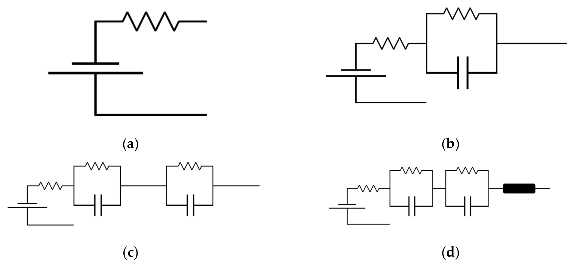
Figure 2.
Plots for 25C04 at state V and cycle 39 a) DRT, b) Nyquist plot.
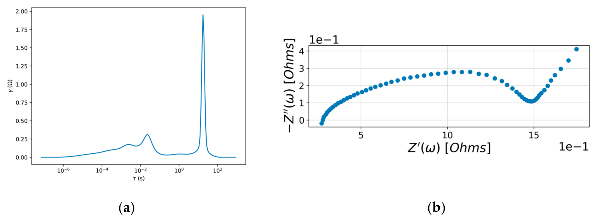
Figure 3.
Clustering Output for each cell with different method on state V; a) 25C04, b) 25C06, c) 25C07, d) 25C08.
Figure 3.
Clustering Output for each cell with different method on state V; a) 25C04, b) 25C06, c) 25C07, d) 25C08.
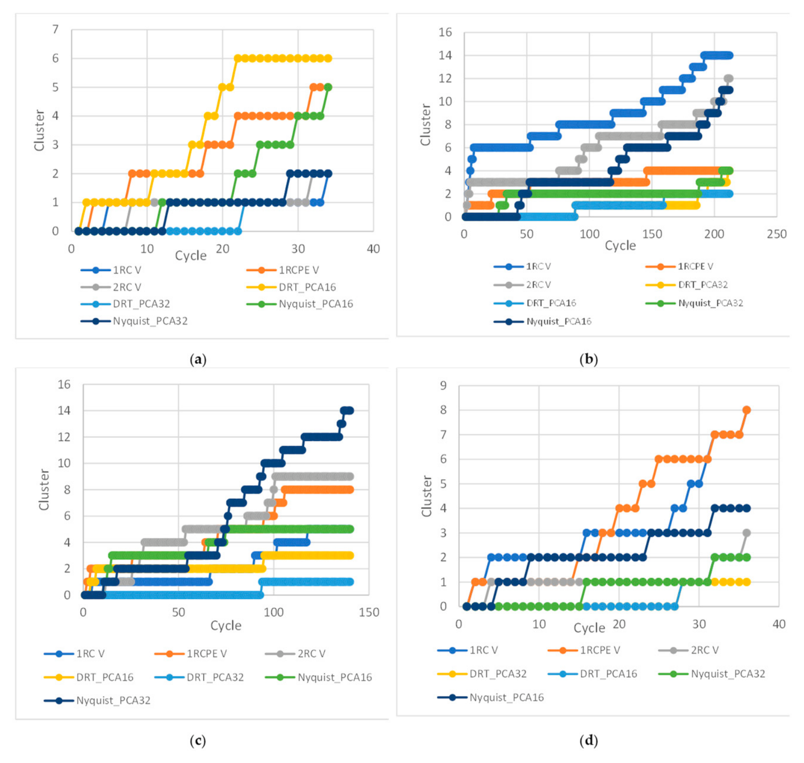

Table 1.
ECM topologies used in this study.
| Model | Elements | Parameters | Physical interpretation |
| 1R | R0 | 1 | Ohmic Resistance |
| 1RC | R0 + (R1‖C1) | 3 | + one polarization / charge-transfer process |
| 1RCPE | R0 + (R1‖CPE1) | 4 | Charge-transfer process with non-ideal (distributed) capacitance |
| 2RC | R0 + (R1‖C1) + (R2‖C2) | 5 | + a second polarization process (e.g., diffusion/SEI) |
| 2RCPE | R0 + (R1‖CPE1) + (R2‖CPE2) | 7 | Two non-ideal polarization processes |
| 2RCPEW | R0 + (R1‖CPE1) + (R2‖CPE2) + W | 9 | + Warburg element for low-frequency diffusion |
Table 2.
Mean absolute PCC (|PCC|) between fitted ECM parameters and SOH, by model and operating state, and Best Parameter for each topology-state pair.
Table 2.
Mean absolute PCC (|PCC|) between fitted ECM parameters and SOH, by model and operating state, and Best Parameter for each topology-state pair.
| Model | State | |PCC| | Best Parameter [Ω] |
| 1RC | V | 0.744 | R0 |
| 1RC | IV | 0.719 | R0 |
| 1RCPE | V | 0.717 | R1 |
| 1RCPE | IV | 0.592 | R1 |
| 1RCPE | IX | 0.586 | R1 |
| 1R | VII | 0.573 | R0 |
| 2RC | I | 0.553 | R0 |
| 1RCPE | I | 0.539 | R1 |
| 1RC | IX | 0.527 | R0 |
| 2RC | IX | 0.509 | R0 |
| 2RC | V | 0.494 | R2 |
| 2RCPE | V | 0.397 | QCPE2 |
| 2RCPEW | V | 0.397 | R2 |
Table 3.
GPR output for ECM-based features with and without cluster feature.
| ECM Model | State | Clustering | MAE | RMSE | STD of errors | MPIW | Coverage (%) |
| 1RC | V | Yes | 0.023 | 0.028 | 0.0275 | 0.114 | 97.22 |
| 1RC | V | No | 0.043 | 0.051 | 0.028 | 0.304 | 97.22 |
| 1RCPE | V | Yes | 0.018 | 0.025 | 0.024 | 0.086 | 91.66 |
| 1RCPE | V | No | 0.020 | 0.031 | 0.026 | 0.084 | 88.88 |
| 2RC | V | Yes | 0.022 | 0.026 | 0.024 | 0.071 | 63.88 |
| 2RC | V | No | 0.019 | 0.024 | 0.024 | 0.086 | 91.66 |
Disclaimer/Publisher’s Note: The statements, opinions and data contained in all publications are solely those of the individual author(s) and contributor(s) and not of MDPI and/or the editor(s). MDPI and/or the editor(s) disclaim responsibility for any injury to people or property resulting from any ideas, methods, instructions or products referred to in the content. |
© 2026 by the authors. Licensee MDPI, Basel, Switzerland. This article is an open access article distributed under the terms and conditions of the Creative Commons Attribution (CC BY) license (http://creativecommons.org/licenses/by/4.0/).
Copyright: This open access article is published under a Creative Commons CC BY 4.0 license, which permit the free download, distribution, and reuse, provided that the author and preprint are cited in any reuse.