

Submitted:
10 October 2026
Posted:
12 October 2026
You are already at the latest version
Abstract
We analyze a specified finite-dimensional chiral operator-spectral candidate whose conservative sector consists of one positive spectral scale and four Hermitian family quadratic forms relative to a common family metric. We first prove that common positive rescaling preserves conservative mass ratios and static spectral subspaces, while simultaneous congruence of the family forms and metric preserves generalized spectra and metric-normalized overlaps. For the evaluated candidate, an analytic neighborhood criterion and its reproducible numerical realization show that every tuple within spectral-norm radius 2.5 × 10⁻² of the four canonical family operators remains outside enlarged charged-lepton, CKM, PMNS reactor-entry, and electron-anchored tritium-endpoint acceptance regions. At this radius the muon-to-electron ratio is below 1.864, the best-permuted CKM distance exceeds 0.248, every admissible static electron-row neutrino overlap exceeds 0.245, and the lightest neutrino rest energy exceeds twelve tritium endpoints after electron anchoring. We then derive relabeling-independent lower bounds on the total reduced pole correction in a fixed conservative/counterterm decomposition. For passive self-adjoint open complements, the reduced kernel is operator-valued anti-Herglotz and the subthreshold pencil is strictly Loewner monotone; under the stated passive hypotheses this yields existence, uniqueness, positive residue, and Lipschitz stability of isolated real pole branches. The finite-dimensional scale and family data define the conservative candidate tested here, while the resulting theorems separate its invariant static limitations from the analytic requirements of a dynamical completion.
Keywords:
fermion masses
; candidate-branch obstruction
; robust operator neighborhoods
; common-metric congruence
; spectral perturbation theory
; matrix self-energy
; Feshbach reduction
1. Introduction
The observed pattern of fermion masses and flavor mixing remains one of the central structural problems of particle physics. In the Standard Model, charged-fermion masses are encoded in Yukawa matrices and become dimensionful after electroweak symmetry breaking [2,3]; nonzero neutrino masses require an extension of the minimal theory, such as a dimension-five Majorana operator or an explicit Dirac/Majorana sector [4]. Once their parameters are supplied, these frameworks describe the measured spectra and mixing data with great precision. Their usual formulation leaves open, however, the common origin of the dimensional mass scale, the numerical hierarchy of the Yukawa sector, and the geometry that relates the family eigenspaces.
These open questions do not signal an inconsistency of established particle theory. They identify a generative problem beyond the parameter-setting content of its conventional formulation: whether the scale and family structure entering the fermion mass problem can arise as correlated outputs of a common underlying dynamics rather than as independent empirical inputs. The parent framework considered here approaches this problem through information projection. Physical sectors are generated by an admissible branch of an eleven-dimensional covariant dynamics, by the stabilization of an active object-supported sector, and by passage to a four-dimensional physical quotient after inactive and nonphysical directions have been removed.
Information projection supplies the generative origin of the physical domain and of the operators defined on it. Their consequences are then developed in the conventional mathematical language of theoretical physics. On the physical quotient, a positive family metric fixes the inner product, second variations of the reduced action define a common scale operator and sector-dependent quadratic forms, and elimination of complementary degrees of freedom produces a retarded reduced kernel. The analysis therefore proceeds from information-projection dynamics to an admissible branch, from that branch to effective operators on a physical quotient, and from those operators to static and retarded spectral statements formulated with positive-operator theory, generalized eigenvalue problems, perturbation theory, propagator poles, and Schur–Feshbach reduction.
The eleven-dimensional parent action, the projection structure, and the seven-block admissible-branch framework are developed in the author’s Version 5.0 monograph, The 11D–4D Covariant Master Equation for a Unified Field Theory [1]. Although the admissible branch has its generative origin in the cited parent framework, the present paper is modularly self-contained as a conditional operator–spectral analysis: its finite-dimensional invariance, obstruction, perturbation, and reduced-pole results follow from the operator data and analytic hypotheses stated explicitly here and can be verified without reconstructing the full eleven-dimensional theory. The present article develops the finite-dimensional diagnostic layer of that program: it identifies the invariant content of the conservative family geometry, proves a robust obstruction for the evaluated static candidate, quantifies the reduced pole displacement required to repair its spectrum, and establishes operator-theoretic conditions for a passive retarded completion. We analyze the specified finite-dimensional branch and its explicitly controlled operator neighborhood.
The conservative input is summarized by
where the common positive scale operator is
and is the physical metric on the three-dimensional family space. The positive Hermitian forms , , describe the sector-dependent conservative geometry. Their canonical metric-normalized representatives are
Here “canonical” denotes the positive-square-root transformation that carries to the identity and thereby fixes the orthonormal representative of each family quadratic form.
Under the common-scale hypothesis, the conservative spectrum is
The common factor fixes the dimensionful orbit, whereas the mass ratios and static eigenspaces are determined by the generalized family spectra. The associated positive conservative mass and rest-energy operators are
The physical spectrum is determined at the poles or spectral edges of the interacting propagator. In a polar family basis, the energy-normalized inverse propagator has the matrix form
The conservative operator fixes the static core, while the matrix-valued retarded self-energy moves the pole positions and eigenspaces and determines widths and residues. Physical charged-current mixing amplitudes additionally involve the corresponding renormalized vertices. The scalar relation
is recovered for an isolated eigenchannel or after a justified local diagonal reduction.
The analysis begins by identifying the quantities that survive common rescaling and common family-coordinate changes. These invariants show that the evaluated static candidate cannot be repaired by either transformation. The exclusion persists throughout a nonzero spectral-norm neighborhood of radius in the four canonical family operators. This robust obstruction yields relabeling-independent lower bounds on the total reduced pole correction required by the displayed conservative core. The final stage characterizes a passive orthogonal Feshbach completion through a positive operator-valued spectral measure; below threshold, the resulting anti-Herglotz pencil is strictly Loewner monotone, which gives existence, uniqueness, positive residue, and Lipschitz stability for isolated real pole branches under the stated hypotheses.
Together, these results turn the static candidate into a falsifiable operator problem. They identify the invariant structure that survives changes of scale and family coordinates, establish the persistence of the obstruction under controlled perturbations, quantify the dynamical burden demanded by the physical spectrum, and constrain the analytic form of a passive retarded completion. In the broader mass-generation program, this diagnostic layer provides invariant tests for microscopic constructions of the common scale, family operators, and retarded kernel from a common physical background.
Section 2 places the construction relative to spectral geometry, dynamical mass generation, and mixed-propagator theory. Section 3 formulates the reduced pole problem. Sections 4–6 develop the conservative operator structure and its invariances; Sections 7 and 8 evaluate the candidate and prove the robust obstruction; and Sections 9–11 develop the reduced dynamics, physical interpretation, and microscopic realization program.
2. Physical Setting and Relation to Established Approaches
2.1. From an Information-Projection Branch to a Conventional Operator Problem
The parent information-projection framework enters the present analysis through a definite generative sequence. An admissible eleven-dimensional branch selects an active object-supported sector, removes gauge, constraint, and inactive directions, and produces a four-dimensional physical quotient on which effective response operators can be defined [1, Version 5.0, Parts K–L]. On that quotient, the reduced action supplies a positive normal response, a common family metric, sector-dependent quadratic forms, and—after the complementary degrees of freedom are eliminated—an energy-dependent retarded kernel. The resulting relation may be summarized as
The first two arrows express the generative content inherited from the parent theory. The remaining arrows are developed here in the standard language of positive operators, generalized eigenvalue problems, perturbation theory, and analytic operator pencils.
This separation of roles is central to the paper. The common metric, the scale operator, the four family forms, and the open-sector response are correlated objects in the parent program rather than unrelated phenomenological matrices. Once a finite-dimensional realization of those objects has been specified, however, its invariant content and its pole structure are ordinary questions of operator theory. The present article begins at this finite-dimensional interface and asks what follows from it without using the phenomenological comparison data to redefine the operator tuple.
2.2. Spectral Geometry and Dynamical Mass Generation
Spectral descriptions of particle masses occur in several established settings. In the spectral-action program, an almost-commutative spectral triple and its finite Dirac operator encode internal gauge, Higgs, Yukawa, and mixing data, while the full spectral action supplies the accompanying gravitational terms [5,6]. Geometric regularity requirements such as Hodge duality can further constrain mass differences and mixing [7]. The present construction shares the premise that flavor data should be treated geometrically, but its finite object is different: one positive scale operator acts on a rank-six physical normal quotient, whereas four positive Hermitian forms act on a common three-dimensional family space. The first question is therefore which parts of this scale–family structure are intrinsic and which are artifacts of a common choice of scale or coordinates.
Dynamical-mass programs based on Dyson–Schwinger equations address a complementary level of the problem. They determine momentum-dependent propagator dressing from field equations, truncations, and renormalization conditions [8]. In the present setting, the static family operators provide the conservative core, while the retarded matrix self-energy supplies the energy-dependent displacement and rotation needed to reach the physical poles. Rather than solving a microscopic Dyson–Schwinger system, the analysis quantifies how far the displayed conservative core lies from the required pole spectrum and determines analytic conditions under which a passive reduced completion is well posed.
2.3. Pole Theory, Flavor Mixing, and the Contribution of This Paper
Complex poles, residues, and mixing in unstable or flavor-coupled systems are standard subjects of resummed propagator theory [9,32,33]. Orthogonal Schur–Feshbach reduction provides the natural retained/open decomposition for the finite-dimensional problem considered here. A passive self-adjoint complement induces a positive operator-valued spectral measure; its Cauchy transform is anti-Herglotz, and matrix-valued Herglotz theory together with Feshbach–Schur estimates controls the subthreshold pole problem [17,18]. The pole eigenspaces obtained from this reduced problem are distinct from the renormalized charged-current amplitudes, which also contain the corresponding interaction vertices and external-state residues.
The contribution of the present paper lies in combining these standard analytic tools with a branch-specific common-metric geometry. Common rescaling and simultaneous metric congruence first identify the invariant static information. That information yields a robust obstruction for the evaluated candidate and for an explicitly controlled operator neighborhood. The same obstruction gives quantitative lower bounds on the reduced pole correction, after which the passive Feshbach theorem specifies an admissible analytic class for the required dynamical completion. The next section states the reduced operator data and proves the pole-identification result on which this sequence rests.
3. The Reduced Operator Problem and Its Analytic Hypotheses
The conservative family geometry and the open complement play different physical roles. The former fixes a common scale, mass ratios, and static eigenspaces; the latter converts that fixed core into an energy-dependent operator pencil whose zeros and residues define the reduced pole data. This section places both structures on one declared physical quotient and states the precise hypotheses under which the Schur–Feshbach identification is valid.
3.1. Conservative and Open Data on the Physical Quotient
The reduced operator data associated with the specified branch are
The first group specifies the conservative geometry. The positive metric defines the inner product on the common family quotient, the four positive Hermitian forms define the sector-dependent static geometry, and the pair determines the common positive scale operator. The coefficient realizes that scale in the dimensionful mass chart used below.
The second group specifies the open complement. For each sector, is a self-adjoint energy operator on a Hilbert space , couples the retained family space to that complement, fixes the Hermitian counterterm in the declared decomposition, and specifies the analytic continuation sheet. The dimensionful factorization introduced in Section 5 may also use the action coordinate ; the minimal pole problem depends only on the combined scale operator
on the physical-normal quotient, together with an isolated lowest spectral cluster.
Definition 3.1
(Conditional reduced pole-identification problem). For fixed , the reduced problem is to construct the canonical scale and conservative rest-energy operators, form the open-sector Feshbach kernels and the total reduced corrections, and identify the isolated zeros and residue operators of the resulting family-energy pencils.
3.2. Analytic Structure and the Finite-Dimensional Realization
Three physical levels meet in this definition. At the analytic level, positivity, self-adjointness, bounded retained–open coupling, and meromorphic continuation determine the spectral calculus, the Schur–Feshbach factorization, and the pole and residue formulas. At the finite-dimensional level, the evaluated scale representation and family forms supply one concrete conservative geometry to which the invariance and obstruction theorems can be applied. The numerical relations
are consistency relations among the provided finite-dimensional representations of that fixed quadratic data. At the microscopic level, a common-background realization must generate the physical quotient, its normalization, the four family forms, and the open spectral measure from one stationary parent branch with compatible conventions.
The roles of the inputs used in the main argument are summarized in Table 1. Detailed data identifiers, input-dependence records, and numerical reproduction instructions are collected in the Supplement, while phenomenological masses, mixing data, and endpoint bounds enter only as tests of the invariant outputs.
A full relativistic flavor calculation extends this hierarchy. It requires the Dirac–family form factors , the relevant gauge identities, external-state residues, and renormalized charged-current vertices. The reduced family pencil is therefore the operator-theoretic interface between the finite-dimensional geometry and the complete 1PI amplitudes.
3.3. Schur–Feshbach Identification of Poles and Residues
The following proposition states the exact reduced result. Its assumptions separate the conservative positivity conditions from the analytic conditions on the open complement and from the simplicity condition required for a rank-one residue.
Proposition 3.2
(Conditional reduced pole identification and Schur–Feshbach lift). For each sector let the retained space be and the open space be a Hilbert space . Assume that the reduced branch datum in Equation (8) satisfies:
- (a)
- on the physical-normal quotient and its lowest eigenvalue is isolated from the rest of the spectrum;
- (b)
- , , and with ;
- (c)
- is self-adjoint on , is bounded, and ;
- (d)
- on a connected domain of the specified sheet , the open resolvent and the reduced pencil below admit a meromorphic continuation;
- (e)
- each pole to which the residue formula is applied is a simple characteristic value:
Define
The corresponding block operator on is
For the Schur–Feshbach factorization is
Hence is invertible if and only if is invertible. Moreover,
with equality of kernel dimensions. In finite dimensions the same statement may additionally be written as the usual determinant identity.
At a simple characteristic value,
and is rank one but is not generally idempotent. For an isolated bound-state eigenvalue of the linear block operator, the Riesz projector is
Write the reduced characteristic value as , and define and . These reduced quantities agree with relativistic pole quantities when a pole-preserving matching has been established on the specified analytic branch.
Proof.
Finite-dimensional spectral calculus gives the canonical scale and conservative mass operators. Self-adjointness of and boundedness of define the physical-sheet resolvent and the positive measure ; the assumed continuation supplies the meromorphic pencil on . Direct multiplication proves Equation (17), and therefore the equivalence of invertibility, the equality of kernel dimensions, and the full-state lift Equation (18). Standard analytic matrix-pencil theory at a simple characteristic value gives the Laurent coefficient Equation (19), while the contour formula gives the ordinary Riesz projector of the underlying linear operator. The proposition thus identifies the poles and residues of the declared reduced problem and fixes the additional matching required for their relativistic interpretation. □
Corollary 3.3
(Identification from specified reduced data). For fixed and a specified analytic sheet, every isolated simple zero of the reduced pencil has the pole, full-state lift, and residue representation in Proposition 3.2. A subthreshold existence–uniqueness theorem under stronger passive hypotheses is proved in Theorem 9.2.
3.4. From Reduced Identification to a Common Microscopic Origin
The proposition solves the spectral identification problem once the reduced data have been fixed. The generative program asks how those data arise together. A microscopic realization from a common physical background must obtain , , the common quotient, the four family forms, the normalization, and the open spectral measure from one stationary parent solution rather than from separately chosen constructions. Equality of the final finite matrices is a necessary consistency check, but the common physical origin is encoded in their shared domain, root, normalization, and retained/open decomposition.
The hierarchy of claims used throughout the paper is
The next sections develop the conservative part of this hierarchy: the canonical scale operator, the common family metric, the four sector forms, and the invariants that will later support the obstruction theorem.
4. Generation of the Common Scale and Family Geometry
The conservative fermion problem begins on a physical domain selected by the parent information-projection dynamics. After gauge, constraint, reparametrization, rigid-motion, inactive, and redundant readout directions have been removed, the specified branch leaves two finite-dimensional response spaces with different physical roles. A rank-six normal quotient carries the response that fixes the common dimensional scale, whereas a three-dimensional family quotient carries the relative hierarchy and orientation of the four fermion sectors. The two spaces are not alternative descriptions of one vector space. They are correlated outputs of the same reduced branch and are linked only through the common scale relation developed below.
4.1. The Physical Quotient and the Common Scale Response
Let denote the canonical-electron physical normal quotient of the finite-dimensional realization studied here. The quotient is the domain on which physically distinct normal deformations remain after the nonphysical directions have been eliminated. On this domain, is a strictly positive support/area quadratic form and is a self-adjoint normal-tension quadratic form. Their coordinate-independent combination is
The dimensions are fixed by
Thus measures the geometric support of a physical normal deformation, measures the energy cost per unit length of that deformation, and is the positive response operator that combines them. The separate normalizations of area and tension are representational; the spectrum of their product is the physical datum used by the conservative mass construction.
A normalized operator shape does not fix its dimensionful scale: for fixed , the family , , has identical normalized geometry and different dimensionful spectra. Thus the rank-six shape fixes relative stiffness and degeneracy data, whereas the positive scale coefficient is supplied by the dimensionful realization in Section 7.
Assumption 4.1
(Positive isolated canonical scale operator). is positive and self-adjoint on the finite-dimensional space , and its lowest eigenvalue
is positive and isolated. The associated Riesz projector is denoted .
The scalar provides the lowest positive response carried by the rank-six quotient. If the lowest cluster is degenerate, the invariant object is the full Riesz subspace: individual basis vectors inside that subspace depend on the chosen coordinates, whereas the spectral value, its multiplicity, and the projector do not.
4.2. Coordinate Covariance and Factorization Independence
The physical scale response must be independent of both the basis chosen on and the auxiliary factorization used to represent it. The first statement is ordinary unitary covariance.
Lemma 4.2
(Unitary covariance). For a unitary transformation U on ,
implies
Consequently , the multiplicity of the lowest cluster, and the transported Riesz projector are basis invariant.
Proof.
The second statement concerns the split into support and tension. It changes the two factors reciprocally while leaving the combined response fixed.
Proposition 4.3
(Area–tension refactorization). For every ,
leaves exactly unchanged.
Proof.
Because ,
□
The proposition identifies the combined scale operator as the factorization-independent quantity. Choosing separate absolute normalizations for and is an additional convention and cannot alter , , or the physical normal subspace.
4.3. The Family Metric and Sector Quadratic Forms
The relative fermion data live on a different quotient. Let be the common active family space of the same specified branch, equipped with the positive physical metric . The metric determines lengths and angles in family space. Each sector is represented by a positive Hermitian quadratic form
on that common metric space. Passing to the canonical -orthonormal frame gives
with and . Equivalently, solves with . In the orthonormal family frame used for the numerical realization, , so the printed forms coincide numerically with their canonical representatives.
The spectra of encode the sector-dependent hierarchy, while their spectral subspaces encode the relative family orientation. The lowest electron eigenvalue is taken to be simple,
which fixes the electron eigenline up to phase. If a family eigenvalue is degenerate, the invariant datum is again the Riesz subspace and the principal angles between subspaces rather than any particular eigenbasis.
The conservative architecture separates this relative geometry from one common positive scale. With a single scalar shared by all four sectors,
so the absolute level changes coherently while the spectral ratios and eigenspaces remain sector dependent. This is the precise sense in which the branch contains one dimensional scale but four distinct family geometries.
4.4. From the Scale Response to the Dimensionful Anchor
The rank-six scale response enters the family spectrum through the canonical absolute anchor
Here is the lowest positive scale response and is the common inverse-length conversion supplied by the finite-dimensional branch. For the realization studied in this paper,
The factor is the baryon-to-photon occupancy ratio of the BBN branch and is consistent with the Planck 2018 cosmological-parameter analysis [29]; the other quantities are the canonical-electron, readout, and global-screen inputs that define the same dimensionful chart. Their numerical values are
All four sectors use this same conversion. The printed digits specify the numerical realization reproducibly; the physical precision is controlled by the least precise input and by the joint covariance of the underlying branch data.
The outcome of this section is therefore a clean separation of roles. The quotient and the operator provide the common dimensional response; the metric space and the four forms provide the relative family geometry. The next section derives the conservative spectrum and identifies the information that no common change of ruler or family coordinates can alter.
5. Static Spectrum and Invariant Family Data
The scale–geometry separation of the previous section immediately organizes the conservative spectrum. One scalar fixes the common dimensionful orbit, while the eigenvalue ratios, spectral subspaces, and relative family orientations are determined by the four quadratic forms. This section derives that spectrum and proves the two invariance statements that later make the static obstruction possible.
5.1. The Electron Anchor and the Common Conservative Spectrum
The family spectra are those of the canonical metric-normalized endomorphisms
The numerical realization is already written in a -orthonormal frame, for which and the printed sector forms equal their canonical representatives.
Assumption 5.1
(Common positive chiral scale). The four conservative canonical mass-square endomorphisms are related to the evaluated candidate endomorphisms by one sector-independent positive scalar,
and the first electron mode is anchored by
Lemma 5.2
(Unique positive common scale). Under Assumption 5.1,
is the unique positive common scale.
Proof.
Because , the electron anchor equation has exactly one positive solution. □
Proposition 5.3
(Electron-anchored common-scale relation). Under Assumptions 4.1 and 5.1, the conservative fermion masses are
Equivalently,
Proof.
Insert Equation (39) into , and then use . □
The proposition exhibits the two pieces of the conservative spectrum directly: sets the common ruler, and the normalized family eigenvalues fix the relative positions of the modes. Removing the ruler therefore leaves every ratio unchanged.
Corollary 5.4
(Common-scale-independent ratios). For any two conservative modes,
All conservative mass ratios are independent of , , , and of the factorization chart used for the common action normalization.
This scale-free hierarchy is the first obstruction invariant used later: a candidate with incorrect generalized eigenvalue ratios cannot be repaired by adjusting its common absolute scale.
5.2. Family Subspaces and Static Mixing Data
The same separation holds for the conservative eigenspaces. In the canonical orthonormal family frame, define
These overlap constructions are the static analogues of the Cabibbo–Kobayashi–Maskawa and Maki–Nakagawa–Sakata matrices [10,11,12]. If is instead written in the original metric frame, with and , then and . Thus the overlap information is intrinsic to the metric geometry, not to the coordinates used to display it.
Theorem 5.5
(Static overlap data under common scaling). At fixed , a common positive rescaling of all four family quadratic forms leaves every simple spectral subspace unchanged. With a covariantly transported phase convention the representatives in Equation (43) are constant; without fixing that gauge, the invariant statements concern the rephasing class, entrywise moduli and closed-cycle invariants, or, for degenerate clusters, the associated projectors and principal angles.
A common scale therefore changes neither the conservative family axes nor their relative angles. These static overlaps enter physical CKM- or PMNS-type amplitudes only when the pole corrections, residues, and charged-current vertices preserve the relevant subspaces. A sufficient local condition for the self-energy part is
in a neighborhood of the pole, together with residue matrices that are diagonal in the same basis.
5.3. Common Congruence and Geometric Invariants
Changing the common scale and changing family coordinates are distinct operations. A scale transformation changes the physical ruler. A simultaneous congruence transformation rewrites all sector forms and the family metric in one new coordinate frame. In the original metric variables, the generalized eigenproblems are
The corresponding metric overlap is
Theorem 5.6
(Common-metric congruence invariance). Let and be common to all four sectors, and define
If the physical support quotient is unchanged, then the generalized eigenvalues are invariant and, for the covariantly transported eigenframes in Equation (49), the metric-normalized overlap representative is unchanged:
A normalized transformed eigenframe is
Moreover, with
is unitary and the canonical family endomorphisms obey
Hence the positive canonically normalized mass and rest-energy operators transform unitarily rather than by a noncovariant ordinary square root of .
Proof.
Substitution gives
The theorem gives the geometric meaning of the common congruence: it changes the coordinate grid but not the generalized spectra or the relative family geometry. Consequently, the invariant mismatch of the specified static candidate cannot be removed by a common change of family basis. It can change only through a sector-dependent deformation, a change of physical support, or an energy-dependent correction that fails to commute with the static forms.
5.4. Action Normalization and the Absolute-Scale Orbit
The dimensionful action normalization may itself be factorized without changing the physical scale operator. Introduce one positive action normalization
and write
Then
and
The reciprocal change
is only a refactorization of the same physical operator: , , and every mass remain fixed. By contrast, a physical common-scale transformation keeps fixed and changes . It moves the entire spectrum along its one-dimensional absolute-mass orbit while preserving every ratio and every static family overlap. This is the operator-theoretic form of the distinction used in the Conclusion: changing the ruler is not the same as changing the geometry drawn with it.
5.5. Chiral Interpretation of the Positive Family Operators
The positive family operators determine the left spectral data entering the static analysis, while the full chiral interpretation depends on the fermion sector. For a Dirac sector,
The positive left operator fixes the singular values and left spectral subspaces but leaves the independent right-handed rotation undetermined. In the polar family basis used for the pole analysis, the conservative Dirac mass representative is the positive Hermitian operator and its rest-energy form is ; in a general chiral basis the lift is .
For a Majorana sector,
is a Takagi factorization. The positive operator again determines the masses and left spectral subspaces, while the complete CP-sensitive content requires the full Majorana matrix. The conservative results proved in this section therefore concern the positive spectra and their metric geometry; the retarded self-energies and vertices introduced later complete the pole positions, residues, and physical mixing amplitudes.
The static layer is now fully specified. The next section compares the several geometric and information-theoretic representations of the same common scale and determines which equalities are physical identities and which are consistency checks of the finite-dimensional realization.
6. Equivalent Representations of the Common Scale
The preceding sections separated the common dimensionful scale from the relative geometry of the four family sectors. This section compares four normalized descriptions on the same six-dimensional quotient: a boundary shape response, the stationary Hessian of the reduced action, a BKM information-geometric response, and an area–tension factorization after electromagnetic carrier projection. In the evaluated finite-dimensional realization their normalized operators agree within the stated tolerance. The analysis uses that agreement as a consistency relation for the candidate scale structure, not as four independent contributions to be added to the mass.
6.1. Boundary Geometry and the Shape Response
The six normal directions acquire a direct geometric meaning once the electron sector is represented by a finite event group with an endogenous boundary. Let with be the normalized event density on a spatial slice, and define its centroid by . We assume
and choose a regular branch value for which the superlevel set has a compact smooth boundary,
The boundary is therefore generated by the stabilized event density rather than inserted as an unrelated external surface. After translations, rotations, gauge directions, reparametrizations, constraints, and redundant readout directions have been removed, an admissible normal deformation is written
where the six functions span the physical normal quotient of the specified realization. Their number is an independent property of that quotient and is not inferred from the rank-three covariance in Equation (60). Since the coordinates are dimensionless, the functions carry length dimension. With a fixed reference length , , and , the natural positive metric on the deformation space is
The reference length fixes the coordinate convention on the normal quotient; it is not a sector-dependent adjustment of the physical spectrum.
Let be the conservative boundary normal-flux functional, including the branch boundary subtraction and counterterm terms, and normalized so that its second derivative with respect to the dimensionless shape coordinates has units . The reversible auxiliary variables a are determined by the stationary envelope . The physical shape response is then
Because the auxiliary variables relax jointly, the envelope theorem produces the same sum-before-Schur structure that will appear in the stationary action. Raising one index with the deformation metric gives the coordinate-independent operator
Proposition 6.1
(Conditional shape-Hessian/area–tension compatibility). Assume there is a unitary identification between the canonically normalized normal quotient and the canonical scale-operator support such that the two constructions represent the same Riesz endomorphism,
Then
so the two operators have the same spectrum and the same lowest stiffness .
Proof.
The conclusion is immediate from the explicit common-Riesz identification Equation (65). Covariance of a shape Hessian under changes of deformation coordinates guarantees unitary transport once the common Riesz endomorphism is specified; it does not by itself prove that an independently defined area–tension pair represents the same endomorphism [36]. □
In the finite-dimensional realization studied here, the two sides of Equation (65) agree to the numerical precision of the supplied operators. Under this identification, is the lowest conservative stiffness of the admissible electron-boundary deformations. Thus the scale operator has a geometric boundary interpretation, while its independent production from a complete eleven-dimensional boundary-value problem remains a separate microscopic construction.
6.2. Action and Information Representations on the Normal Quotient
The same six-dimensional response can be read from the reduced action and from the distinguishability geometry of the locked state family. These descriptions are physically meaningful only after they have been placed on the same normal quotient and normalized with their respective metrics.
Let denote the six physical normal coordinates and a the reversible stationary auxiliary variables. The seven conservative action blocks are first added, , and only then are the shared auxiliary variables eliminated. If has locally constant rank and on the stationary branch, the envelope Hessian is
and its metric-normalized action representation is
This operator measures the conservative cost of a physical normal deformation after every reversible internal coordinate has relaxed at the same stationary point.
The statistical description starts from a locked family of states on the same physical quotient. The BKM metric is the Hessian of relative entropy on that family [23,24]; it measures local distinguishability, while the source Hessian measures the response induced by the corresponding source directions. Their normalized operator is
We write for numerical equality in the evaluated finite-dimensional realization at the precision of its stored operators. The two representations give
with relative operator defect
The action and BKM constructions therefore agree as normalized finite-dimensional operators in this realization. This numerical equality is the consistency relation used here. A stronger microscopic identification would require the action Hessian and the information-geometric response to be obtained independently from their respective variations before the two operators are compared.
6.3. Carrier Projection and the Area–Tension Form
The preceding operators act on the six-dimensional physical normal quotient. To identify the electromagnetic component, the normal response must also be paired with the internal carrier decomposition. Equip the carrier with
Then
are orthonormal carrier directions in the standard decomposition [31]. The visible electromagnetic line is represented by
Its unit representative is
Hence the squared weight of the central trace direction is
while the traceless complement carries weight .
Assumption 6.2
(Canonical electromagnetic component assignment). In the canonical-electron readout branch, the normalized central component is assigned to the electromagnetic component of the scale operator, while the orthogonal component is retained in the traceless color-complement sector. The two components belong to distinct projected sectors, and each is counted once. In addition, the evaluated carrier-to-shape map is assumed to be diagonal in the decomposition, with the same rank-six shape block for both carrier components and no mixed carrier–shape cross term. Under this separability condition the carrier projection acts on the shape stiffness by the scalar weight .
The normalized carrier projection therefore sends the common action response to the electromagnetic shape operator,
The same positive operator has an area–tension factorization. In the evaluated representation,
so that
The trace-projected action operator and the area–tension factorization agree to a relative numerical defect below . Collecting the action, information, carrier, and factorized descriptions gives
Equation (81) identifies alternative representations of one candidate quadratic response. They are neither added nor multiplied as independent mass contributions.
6.4. Prospective Common-Background Energy Identities
The scale operator also admits local and global energy representations when the clock, source, and spectral variations are all derived on one stationary electron background. In this subsection, denotes the action coordinate whose SI representation is specified in Equation (89). On a reversible one-cycle branch, let be the local proper-time readout factor and define the proper modular acceleration
If the same branch has reversible lock entropy , if the rest energy equals the reversible modular cost , and if the effective modular temperature obeys the Unruh-normalized acceleration relation
then [25]
Consequently,
Equating the spectral and modular expressions gives
A global representation is furnished by the trace-reversed source energy
Independent local-gradient, source-volume, and spectral variations on one stationary background would then satisfy
This equality is a closure condition linking local clock response, integrated source energy, and the spectral scale when all three are evaluated on one stationary electron background. The obstruction analysis below uses the spectral realization in Equation (40); the local-gradient and source-volume expressions provide independent cross-checks for a microscopic completion. We next place the common scale in a dimensionful chart and apply it, without sector-dependent readjustment, to the four family operators.
7. Dimensionful Realization and the Four-Sector Static Candidate
The preceding operator identities separate the common scale from the relative family geometry. The limited dimensional-realization principle needed here is that one physical scale quantity may admit equivalent factorizations, while a chosen unit chart supplies its numerical coordinate rather than an additional dynamical factor [40]. This section expresses the specified scale operator in two such coordinates, uses the electron line as the common anchor, and then evaluates the conservative spectra and eigenspaces of all four sectors. The same scale is used throughout; every inter-sector difference comes from the canonical family operators.
7.1. One Scale Operator in Two Factorization Coordinates
In the full-amplitude coordinate, the declared action coordinate is represented in the SI chart by the reduced Planck constant,
The SI definition fixes h exactly and therefore fixes exactly; the displayed digits are its decimal expansion. Here is the numerical action coordinate of the declared chart. The specified mass–action realization supplies the branch-dependent dimensionless amplitude
Together, and represent the dimensionful common-scale operator in the full-amplitude coordinate. The same operator can be written in a canonical-electron shape coordinate. Since
the amplitude multiplying the normalized shape is
Transferring this amplitude from the dimensionless operator to the action coordinate gives
The two coordinates reconstruct exactly the same dimensionful operator,
Thus and are not two action quanta. They are alternative factorization coordinates of one positive scale response and are never multiplied or averaged as separate mass factors.

Table 2.
Two factorization coordinates of the same dimensionful canonical-electron scale operator.
| Quantity | Full-amplitude coordinate | CE-shape coordinate |
| Action coordinate | ||
| Dimensionless operator | ||
| Lowest eigenvalue | ||
| Invariant operator |
The common operator has the spectral bottom
Combining it with Equation (34) yields the common mass anchor
The two factorization coordinates therefore lead to one electron-anchored scale and introduce no sector-dependent normalization.
The central value provides a direct consistency check of the adopted dimensionful chart. The realization gives
whereas the 2026 Particle Data Group central value is
Using the compilation in [27], the fractional central-value difference is
The absolute scale is already contained in the specified mass–action realization, so this comparison tests the consistency of its SI expression rather than supplying an independent scale determination. The numerical table below fixes the static candidate on which the obstruction theorems act: those theorems use its scale-free ratios and eigenspaces, while the electron comparison locates the candidate on the adopted SI scale. A complete uncertainty analysis would additionally propagate the covariances of , , , , and .
7.2. Conservative Spectra of the Four Sectors
Once the common anchor is fixed, Equation (40) maps the four canonical family spectra to the conservative mass candidate in Table 3. The same is used for every row; no sector is separately rescaled.
The table is a static output of the four-sector operator realization. The u- and d-sector eigenvalues require either a specified short-distance quark-mass scheme or a gauge-invariant color-singlet spectral observable before they can be compared with physical quark masses, because confinement and the infrared renormalon obstruct a direct pole-mass interpretation [30]. The neutrino row is likewise the conservative spectrum of the displayed operator. Its active-neutrino kinematics, and the charged-lepton hierarchy of the same realization, are tested by the invariant obstruction analysis in Section 8.
7.3. Static Eigenspaces and Overlap Geometry
The eigenvectors of the same canonical family operators define the relative orientation of their static spectral subspaces. In the canonical -orthonormal frame, the entrywise moduli of the resulting overlap representatives are
The moduli in Equations (100) and (101) are rounded for readability. Higher-precision signed orthogonal representatives are printed in Appendix C; the Frobenius norms of their unitarity defects are and . These matrices are the static overlap geometry of the conservative candidate. Their identification with physical CKM- or PMNS-type amplitudes requires the pole eigenspaces and the corresponding renormalized charged-current vertices. The next sections therefore use them first as invariant diagnostics of the static branch, and then compare that branch with the energy-dependent pole problem.
8. Robust Static Obstruction and Minimum Dynamical Burden
The conservative candidate can be tested before any microscopic open-sector kernel is chosen. Its charged-lepton ratios and static overlap geometry depend only on generalized spectra and eigenspaces, while the neutrino endpoint test becomes definite once the single common scale is fixed by the electron anchor. The invariance results of Section 5 therefore turn the numerical comparison into a structural question: whether the displayed family geometry can represent the observed flavor sector under the transformations already allowed by the theory.
Definition 8.1
(Direct-static identification premise). For the tests in this section, direct-static identification means that the physical pole subspaces are identified with the displayed conservative subspaces, the renormalized charged-current vertex introduces no compensating family rotation, and only the explicitly stated relabelings and rephasings are applied.
Under this premise, the charged-lepton hierarchy, CKM overlap, and PMNS reactor entry are fixed by scale-free spectral data. The active-neutrino endpoint test is read after electron anchoring. Thus the common parameters , , and set the overall dimensionful orbit but cannot alter any of the four diagnostics below.
8.1. Scale-Free Diagnostics of the Conservative Geometry
Charged-lepton hierarchy. The static branch gives
The reference ratios are approximately
These ratios follow from the PDG and CODATA reference values [27,28]. The static charged-lepton hierarchy is therefore incompatible with direct identification. Retaining the displayed conservative electron anchor, the corresponding same-label conservative-to-pole energy differences for the other two modes are
These same-label differences are only a first indication of the displacement demanded by the observed poles. The operator bound at the end of this section removes the dependence on a chosen mode assignment and gives the corresponding minimum burden in norm.
Quark overlap and CP. The PDG CKM moduli are approximately
We tested all independent row and column permutations of . The best permutation is
with
No relabeling of the three static axes brings the displayed quark overlap close to the physical CKM pattern. The comparison probes the left-eigenspace geometry; a quark mass-hierarchy test would additionally require a common short-distance mass scheme and scale. Because the evaluated u- and d-sector forms are real symmetric, their central static overlap is real orthogonal and hence
The observed CKM sector has nonzero CP violation [27], so the displayed central real candidate cannot reproduce that phase invariant. A complex noncommuting pole correction or a nontrivial renormalized charged-current vertex is required for a CP-active completion. Equation (108) is an exact obstruction for the central real branch; it is not asserted for the full complex-Hermitian perturbation neighborhood.
Leptonic reactor entry. Global neutrino fits give
These representative values are from the PDG neutrino-mixing review [27]. The simple lowest charged-lepton eigenmode is fixed as the electron anchor, so charged-lepton row permutations are not admissible; only neutrino-column relabelings are allowed. The smallest entry in that electron row of is
With the electron row fixed, no neutrino-column relabeling produces the observed small reactor entry. The mismatch is therefore a property of the displayed static eigenspaces rather than of the common mass normalization.
Active-neutrino endpoint kinematics. The tritium beta-decay endpoint is approximately
The displayed static neutrino masses satisfy
Because the static electron row has no vanishing entry, each of the three displayed modes couples to the electron-flavor charged current. If these were the only three active neutrinos, tritium beta decay would have no kinematically allowed neutrino final state. This endpoint obstruction is the primary exclusion and does not rely on the light-neutrino effective-mass approximation [35].
For an auxiliary common-scale-invariant diagnostic, define the electron-anchored RMS ratio
The KATRIN light-active bound at confidence level, together with the PDG electron mass, gives
The displayed formal ratio exceeds this scale by . Because the candidate masses already exceed the tritium endpoint, the endpoint argument is the physical exclusion. Equations (113) and (114) are retained only as an electron-anchored order-of-magnitude diagnostic and are not counted as an independent second exclusion.
8.2. Invariant Obstruction and Its Operator Neighborhood
The preceding diagnostics now combine into a single invariant statement. Common scaling changes the ruler, and common congruence changes the family coordinates, but neither transformation changes the ratios and relative spectral subspaces that fail the direct-static tests.
Theorem 8.2
(Static candidate-branch obstruction theorem). Under the direct-static identification premise in Definition 8.1, no common positive scalar rescaling of the displayed conservative family operators that is simultaneously fixed by the physical electron anchor can reproduce the charged-lepton hierarchy, the CKM pattern, the PMNS reactor entry under the fixed electron-row premise, and the tritium-endpoint kinematics.
Proof.
The common scalar cancels exactly from the charged-lepton ratios and does not change the static CKM or PMNS eigenspaces. It also leaves the theoretical ratios invariant. Once the common scale is fixed by matching the electron anchor to the measured electron mass, those fixed ratios imply the tritium-endpoint obstruction. The direct endpoint statement is therefore an electron-anchored physical exclusion, not an absolute invariant of an unconstrained common-scale orbit. The KATRIN comparison above is a supplementary scale diagnostic only. □
The common scale is therefore not the source of the flavor mismatch. Retaining the displayed family forms requires a dynamical pole sector capable of moving their spectrum and, where necessary, their eigenspaces; changing the conservative geometry itself is the alternative.
Theorem 8.3
(Common-congruence obstruction theorem). Under the same direct-static premise, the charged-lepton, CKM, PMNS reactor-entry, and electron-anchored endpoint obstructions of Theorem 8.2 are invariant under every common transformation Equation (47) that preserves the physical family support quotient and the electron-anchor condition. Hence they cannot be removed by a common scalar normalization, a common nonunitary field redefinition, or a common change of family metric coordinates.
Proof.
By Theorem 5.6, all generalized spectra and metric-normalized overlaps are invariant under the common congruence. The charged-lepton ratios, the CKM overlap test, and the fixed-electron-row PMNS reactor-entry test are therefore unchanged. The theoretical neutrino-to-electron ratios are likewise generalized-spectral invariants. After the common scale is fixed by the physical electron anchor, these invariants imply the same endpoint obstruction; the unanchored endpoint inequality itself is not claimed to be scale invariant. The electron-anchored KATRIN comparison remains a formal scale diagnostic rather than an additional theorem premise. □
A finite operator neighborhood.
The pointwise obstruction persists under controlled changes of all four family operators. The analytic statement follows from Weyl and Davis–Kahan estimates; its numerical corollary evaluates the resulting margins for the candidate data. Write the family problem in canonical orthonormal coordinates,
and define the uniform spectral-norm ball
Let and denote the ordered simple eigenpairs of , and let
For , Weyl and Davis–Kahan estimates give
Consequently a complete eigenbasis obeys the phase-aligned Frobenius estimate
Let . For a positive tuple , re-anchor the common scale by , and let the tilded masses and static overlaps denote the observables constructed from that tuple. Define the deliberately enlarged observational acceptance region by
where
These windows are intentionally much broader than experimental uncertainties. In the PMNS reactor-entry condition, the charged-lepton row is fixed by the simple lowest electron-anchor eigenmode and only neutrino-column relabelings are allowed. The endpoint condition is read after the common scale is fixed by the measured electron mass.
Theorem 8.4
(Analytic perturbation-neighborhood exclusion criterion). Let the four evaluated centers have simple spectra and let , with . If
then . Positivity and eigenvalue ordering are preserved throughout the ball.
Proof.
Weyl’s inequality supplies the two eigenvalue-ratio bounds. Phase-aligned Davis–Kahan estimates give the basis bounds and the electron-row entry bound. The triangle inequality remains valid after the permitted permutations and rephasings. The four strict margin conditions therefore contradict the four defining inequalities of , while the hypotheses on preserve positivity and ordering. □
Corollary 8.5
(Reproducible floating-point neighborhood obstruction for the evaluated candidate). Evaluating the hypotheses of Theorem 8.4 from the distributed arrays in standard floating-point arithmetic at gives
with
Relative to the smallest evaluated electron eigenvalue, . These decimal margins are a reproducible floating-point corollary of the analytic theorem, not an interval-arithmetic or directed-rounding certificate.
Proof.
The evaluated eigenvalues, simple-eigenvalue gaps, overlap representatives, and all intermediate margins are tabulated in the reproducibility data. Substitution into the four analytic inequalities gives the displayed values. The smallest margin remains far above the reported eigensolver residuals, but no formal interval enclosure is claimed. □
Corollary 8.6
(Joint operator–metric perturbation bound). In the canonical orthonormal coordinates determined by , let
The naturally metric-normalized perturbed representative
satisfies
Thus and place all four evaluated sectors inside Equation (126); the largest induced radius is . These values are deterministic sufficient perturbation budgets, not statistically calibrated uncertainties or confidence radii.
Proof.
Put . Then and . Splitting into and gives
which proves Equation (133). □
The accompanying numerical data give the eigenvalues, spectral gaps, analytic margins, and diagnostic-specific contact radii in Table 4. The proof itself is the Weyl–Davis–Kahan implication above. The displayed decimals are standard floating-point evaluations of that implication rather than interval enclosures, and the randomized stress calculation is only a supplementary consistency check.
8.3. Minimum Dynamical Burden of Retaining the Static Core
The excluded neighborhood shows that no small deformation of the conservative tuple reaches the enlarged acceptance region. The next estimate converts that geometric separation into a lower bound on the total correction in the reduced pole equation. At this stage denotes the complete correction in a fixed conservative/counterterm decomposition; Section 9 will construct its passive retarded part from an open-sector spectral measure.
Theorem 8.7
(Minimum total reduced pole-correction bound relative to the fixed decomposition). Let be a normal conservative rest-energy operator and write the fixed decomposition as
Let z solve the nonlinear pole equation
Then
Proof.
There is a unit vector x satisfying . Normality gives , while the right-hand side is at most . □
For the displayed charged-lepton core, even allowing an arbitrary relabeling of the three static modes, Equation (137) requires
These lower bounds are respectively and of the physical pole energies. They constrain the total correction in the stated conservative/counterterm decomposition rather than the open-sector contribution in isolation. Within that decomposition, a uniformly small additive correction cannot connect the displayed conservative spectrum to the observed charged-lepton poles.
A complementary eigenspace statement follows in the Hermitian real-part approximation. Let be the unperturbed separation between an isolated static cluster and its complementary spectrum, and suppose . A standard Davis–Kahan separation estimate gives
Therefore a required rotation implies
If , the correction is already non-small relative to the static gap. The estimate applies when the mismatch is carried by a Hermitian rotation of the pole subspace; the renormalized charged-current vertex may instead carry part of the observed mixing structure [37,38]. The static analysis has therefore determined both what common transformations cannot repair and how large the dynamical displacement must be if the conservative core is retained. We now turn to the analytic structure that an admissible reduced completion can possess.
9. Retarded Self-Energy and Admissible Pole Completion
The preceding section fixes the task of the dynamical sector: it must move a robustly excluded static spectrum by a quantitatively non-small amount while preserving analyticity, passivity, and the matrix structure of flavor. We now formulate that task as a pole problem. The full relativistic propagator identifies masses, widths, residues, and external-state subspaces; an orthogonal Feshbach reduction then supplies a controlled family-energy problem whose passive spectral measure constrains the allowed reduced kernel.
9.1. Relativistic Pole Geometry and Physical Mixing
A fermion mass in an interacting flavor system is a property of a matrix-valued inverse propagator, not an eigenvalue of the conservative block alone. Let denote the identity in Dirac space and let be the invariant energy-squared variable. In a general chiral basis the energy-normalized inverse propagator is
This projector ordering is the one consistent with . In the polar family basis, , so the conservative term reduces to . The self-energy is decomposed as
Here are dimensionless family matrices, while have energy dimension. Their common origin and the corresponding chiral and gauge identities belong to the relativistic completion. The reduced kernel used below is the retained family-energy projection of this larger problem. The pole condition is
For Majorana fermions the propagator obeys the corresponding charge-conjugation constraints, and the pole problem must be treated with the symmetric Majorana mixing structure [32,33].
A resonance pole is sought on the outgoing-wave analytic continuation of the retarded propagator. We reserve z for the reduced rest-frame energy variable used in the Feshbach problem and s for the invariant relativistic pole. Define the reduced characteristic value by
For the full relativistic propagator, when s is expressed in energy-squared units, write
The full energy-normalized Dirac determinant is evaluated at the appropriate invariant pole , whereas the scalar reduced equation below uses the rest-energy variable . Whenever both descriptions are asserted to represent the same physical pole, we impose the pole-preserving rest-frame matching on the specified analytic branch; only then may one identify and . Without this matching, is only a reduced-model mass parameter and does not determine the relativistic pole mass. For charged asymptotic particles in QED, the strict one-particle pole is qualified by the familiar infrared/infraparticle structure; operational on-shell masses are defined with the corresponding soft-photon prescription [34]. In confined sectors, the observable must instead be a short-distance mass or a gauge-invariant color-singlet pole/spectral quantity.
At an isolated simple pole, the null space and Laurent residue determine the local external-state geometry. For an analytic inverse-propagator block or reduced pencil , let and be right and left null vectors at a simple zero. The inverse has the local Laurent form
The coefficient of is a finite-rank biorthogonal residue operator and is not generally idempotent. It must therefore be distinguished from a Riesz projector of an underlying linearized operator. Pole subspaces and residue operators determine the external-state basis entering the flavor problem, subject to rephasing, ordering, reciprocal left/right normalization, and unitary rotations inside exactly degenerate pole subspaces.
Pole eigenspaces are necessary but not sufficient for physical CKM- or PMNS-type observables, which are charged-current amplitudes. Schematically,
with the analogous leptonic expression. For stable external states the appropriate conjugation relation between and may be imposed; for unstable mixed states they can bifurcate, and the formula denotes a pole-scheme or amputated-resonance normalization rather than literal asymptotic LSZ states. Consequently, identification of pole subspaces with physical mixing additionally requires the renormalized charged-current vertex and its gauge-consistent residue normalization. The conservative overlaps of Equation (43) survive unchanged only in the commuting, vertex-trivial limit Equation (44); otherwise both the self-energy and the vertex structure can modify the measured amplitudes.
9.2. Feshbach Reduction and the Passive Spectral Measure
To isolate the family-energy channel, let P project onto the retained conservative subspace and . For a block operator
the reduced operator is
The variable z is the reduced rest-frame energy; the invariant relativistic pole remains the variable s of Equation (145). For isolated finite-dimensional eigenchannels, the pole equation reduces to
The Feshbach–Schur block factorization, rather than a full determinant identity, gives isospectral equivalence whenever is invertible; in finite dimensions the same equivalence may also be written as a determinant identity. The notation is reserved for the physical-sheet boundary value on the real axis, and resonance poles require a justified analytic continuation. Purely Q-supported decoupled states have zero P-overlap and are not represented by the reduced channel [13,14,26].
For a passive open complement, the reduced kernel is controlled by a positive operator-valued spectral measure. Before analytic continuation, let the microscopic total Hamiltonian be self-adjoint, let be the open-sector operator, and let map the retained family subspace into the open complement. With the spectral family , define the positive operator-valued measure
After the local kinetic polynomial has been absorbed into the renormalized inverse propagator, define the open-sector Feshbach kernel
and retain a fixed z-independent Hermitian rest-energy counterterm . This realizes the total reduced correction used in Theorem 8.7 as
For with , the Hermitian counterterm has no absorptive part. With the sign convention in Equation (152), is anti-Herglotz (negative Nevanlinna), equivalently is Herglotz–Nevanlinna, and therefore
When a density exists, the boundary value satisfies
The full measure, including possible pure-point or singular-continuous components, is recovered in the weak sense by the Stieltjes inversion formula. A more general analytic subtraction may be retained only if its contribution is written explicitly,
and the subtraction itself obeys the required anti-Herglotz sign condition. No such generalization is invoked in the theorem stated here. Thus real shifts, thresholds, absorptive widths, and residue data are different manifestations of one passive spectral measure and its dispersion relation [13,14,15,16,17,19,39].
Theorem 9.1
(Positive-measure admissibility on the physical sheet). Any microscopic completion obtained by orthogonal Feshbach reduction of a self-adjoint total generator produces an open-sector matrix-valued retarded kernel satisfying Equation (154) on the physical sheet. Conversely, a proposed physical-sheet open-sector kernel whose upper-half-plane or boundary absorptive part violates Equations (154) and (155) cannot arise from such a passive open complement.
No independent residue-sign claim is made here for poles on an analytically continued resonance sheet; the physical-sheet spectral-density statement is the invariant positivity constraint used in this work. The anti-Herglotz sign is necessary but not sufficient for a microscopic relativistic completion: high-energy asymptotics, symmetries, representation content, gauge identities, and compatibility of the full chiral kernels and vertices remain additional constraints.
9.3. Subthreshold Poles, Residues, and Stability
Below the first open threshold the resolvent is self-adjoint and the passive measure makes the reduced pencil strictly increasing in the Loewner order. The pole problem then becomes an ordered spectral crossing, giving a direct theorem for the existence, uniqueness, residue, and perturbative stability of an isolated real branch.
Theorem 9.2
(Subthreshold pole existence, uniqueness, and stability). Let on the open Hilbert space , let , and let the retained space be finite dimensional. Assume that
Define
where and . Then
throughout I. Hence every ordered eigenvalue is continuous and satisfies
If , that ordered branch has a unique zero . If is one dimensional with normalized vector , then the Laurent expansion of the inverse pencil is
and its residue operator is
Finally, let be another pencil on I satisfying the same monotonicity bound and
If the corresponding jth branches cross zero in I, their zeros obey
Consequently, if a sequence of Galerkin or finite-rank reduced pencils converges uniformly on I and, for all sufficiently large indices, preserves the same isolated simple sign-crossing eigenvalue branch inside I, then the corresponding subthreshold pole energies converge with the same explicit error bound.
Proof.
Differentiating the resolvent gives , hence Equation (157). Integration yields ; the min–max principle gives Equation (158). The endpoint signs and strict monotonicity give existence and uniqueness of the zero. For a one-dimensional kernel, analytic matrix-pencil expansion yields Equation (160); its denominator is at least one. Weyl’s bound gives . Combining this with the unit lower slope of both branches gives Equation (162). Uniform convergence, together with persistence of the same isolated simple sign-crossing branch, supplies the final statement. □
Remark 9.3
(Scope). Theorem 9.2 is a physical-sheet bound-state theorem below the first open threshold. It does not assert existence or uniqueness of poles on a complex resonance sheet, where analytic continuation and non-self-adjoint spectral analysis require additional hypotheses.
Equation (152) constrains the reduced family-energy kernel; the full four-form-factor Dirac–chiral self-energy contains additional structure. The spectral weight and the reduced pole width are two readings of the same open-sector coupling and must be counted once. If a survival, form-factor, or resonance filter has already been incorporated into , the same attenuation may not be multiplied a second time into . This no-double-damping rule prevents an apparent fit from being generated by duplicating one physical loss mechanism in both the measure and the denominator.
Expectation-level stability under repeated updates.
A separate stochastic stability criterion may be imposed when the retarded kernel is updated along a sequence of effective states. Let be a nonnegative integrable adapted process measuring the displacement of the family pole geometry from a locked branch after the nth retarded update, and let be deterministic. A sufficient independently assumed stability condition is
Iteration gives
Equation (164) gives contraction in expectation toward a residual floor. It is an additional stochastic hypothesis, logically distinct from anti-Herglotz passivity and Loewner monotonicity, and it does not imply pathwise convergence without further probabilistic control. Once a microscopic covariance and open-sector response are specified, it provides a direct expectation-level stability test.
9.4. From Reduced Admissibility to Microscopic Completion
A predictive completion must derive an upper-half-plane analytic kernel with the appropriate thresholds and continuation sheets from a microscopic current, Hamiltonian, or field-theoretic interaction fixed independently of the target masses. In a stated renormalization scheme it must predict real shifts, widths, and residues together, preserve the applicable gauge identities, and supply the renormalized charged-current vertices needed for physical mixing amplitudes. One interaction structure must govern all modes; assigning separately to each state is not a dynamical theory.
The spectrum in Table 3 remains the conservative core throughout this construction. The static obstruction and burden results of Section 8 determine how far a pole sector must move that core if it is retained, while the present section specifies the analytic structure available to a passive reduced completion. The next sections interpret this static–dynamic separation and formulate the corresponding microscopic tests.
10. Physical Meaning of Static and Dynamical Family Geometry
The preceding analysis separates two physical structures that are often compressed into a single mass matrix. The conservative sector supplies a common dimensionful scale together with four sector-dependent quadratic geometries, while the interacting propagator supplies the energy-dependent pole geometry seen by asymptotic states. The obstruction proved in Section 8 is therefore not merely a failed numerical fit: it identifies which features belong to the common ruler, which belong to the relative family geometry, and which can change only through genuine dynamics.
10.1. The Common Ruler and the Conservative Family Geometry
The positive operator fixes one common scale response. The metric fixes lengths and angles in the three-dimensional family space, and each positive form , or equivalently its canonical representative , defines the conservative quadratic geometry of one fermion sector. The scale operator and the family forms therefore carry complementary information: the former places the candidate on a dimensionful orbit, whereas the latter determine mass ratios, principal subspaces, and the relative orientation of the sectors.
In the evaluated finite-dimensional realization, the action-normal and information-geometric representations obey
This is a consistency relation among normalized representations of the candidate scale structure. The quantities are alternative descriptions of one response and are not additional mass contributions. A stronger microscopic statement would require the action and information forms to be obtained independently from the corresponding stationary action and statistical state.
The dimensionful coordinate used for the evaluated candidate is
These values place the conservative candidate on the declared SI scale orbit. The obstruction results themselves are governed by the resulting mass ratios and spectral subspaces, so their content is not altered by replacing the ruler or by rewriting the same family geometry in another common coordinate frame.
10.2. The Obstruction as a Geometric Statement
A common positive rescaling changes the ruler applied to all four sectors. A simultaneous congruence of the family forms and the metric changes the coordinate grid in which the same generalized geometry is represented. Neither transformation changes the generalized eigenvalue ratios, the Riesz spectral subspaces, or the metric-normalized relative orientations proved invariant in Section 5. In this precise sense, the charged-lepton hierarchy and the static quark and lepton overlap mismatches are properties of the displayed conservative geometry rather than artifacts of normalization or basis choice.
The neighborhood theorem strengthens this statement. It excludes not only one four-operator tuple but every tuple in the proved spectral-norm ball around it. Nearby deformations of the conservative forms therefore remain outside the declared physical acceptance regions. If the displayed core is retained, the charged-lepton poles must be displaced by a correction whose operator norm is comparable to the physical muon and tau energies. This lower bound concerns the total reduced correction in the fixed conservative/counterterm decomposition; it is not a separate assignment of the burden to one microscopic mechanism.
The same distinction clarifies flavor mixing. The conservative forms determine static eigenspaces. The physical external states are instead determined by the poles, residues, and renormalized interaction vertices of the full propagator problem. A self-energy commuting with the conservative operator preserves the static eigenspaces, whereas a noncommuting energy-dependent term can rotate them. The measured CKM- and PMNS-type amplitudes additionally contain the corresponding charged-current vertex factors. A microscopic completion must therefore determine pole subspaces, residues, and vertices as correlated observables of one interaction law.
10.3. From Fixed Quadratic Forms to Pole Geometry
The retarded self-energy promotes the fixed conservative data to an energy-dependent operator pencil. As the invariant energy variable changes, its eigenvalues and eigenspaces may move, and the physical masses are selected where the inverse propagator develops the appropriate poles. The passive Feshbach construction of Section 9 restricts this motion: the physical-sheet kernel has the anti-Herglotz sign, and below threshold the reduced pencil is strictly Loewner monotone. The resulting pole branch is therefore an ordered spectral crossing with a positive residue and controlled dependence on the reduced data.
This static–dynamic separation gives the central physical interpretation of the paper. The common scale organizes one dimensionful orbit, the sector forms define its conservative family geometry, and the open sector completes that geometry at the propagator poles. The next section states what a microscopic realization of this structure must produce and how its claims can be tested without making the present operator theorems depend on the full parent construction.
11. Microscopic Realization and Falsifiable Consequences
The finite-dimensional results proved above require only the positive operators, metric, analytic kernels, and transformation laws stated in this article. A stronger microscopic realization asks for these data to arise together from one stationary physical branch. The purpose of this section is to formulate that additional physical problem in conventional operator and field-theoretic terms and to identify observations that distinguish the candidate calculation from a completed dynamical theory.
11.1. A Common Origin for the Conservative Data
A microscopic construction must produce the physical quotient, its family metric, the common scale response, and the four conservative sector forms before the flavor comparisons are made. In particular, one stationary realization should determine
as quadratic forms relative to the same positive metric , together with the single scale operator . The common scale is then used once for all sectors; sector dependence resides in the generalized spectra and eigenspaces of the family forms.
The action-normal and BKM-normal matrices provide two finite-dimensional consistency representations of this structure. If their equality is promoted to a microscopic identity, the two sides must be computed through their natural variations: the stationary action supplies the action Hessian, while the associated statistical state supplies the information-geometric form. Likewise, the dimensionful realization must respect the declared physical units and normalization rather than introduce a second sector-dependent scale. The accompanying numerical material makes the present matrices and consistency relations reproducible; the additional microscopic task is their joint derivation from one physical solution.
The conservative forms precede the chiral lift to complete Dirac or Majorana mass matrices. Thus a full realization must specify the left- and right-handed representations, the relevant complex phases, and the interaction vertices without changing the common quotient or replacing one sector by an independently normalized construction.
11.2. An Orthogonal Decomposition of Sector Contrasts
The four canonical sector representatives admit a useful exact decomposition into one common coefficient channel and three mutually orthogonal contrast channels in the four-dimensional sector-label space. In the ordered basis , define
with rows denoted (common), (weak-isospin contrast), (color/lepton contrast), and (mixed weak–color contrast). The corresponding coefficient operators are
For the displayed matrices, the reconstruction defect is , and the Frobenius-norm-square fractions are
Because is orthogonal in sector-label coefficient space, the transformation is invertible and preserves the summed Frobenius norm. The matrices remain general Hermitian coefficient operators. Their labels identify algebraic contrasts of the evaluated four-sector tuple; interpreting them as physical weak, color, or mixed generators requires the corresponding symmetry action in the microscopic theory. The explicit matrices are given in Appendix D.
11.3. Retarded Dynamics and Independent Scale Tests
A predictive completion must calculate the matrix self-energy from the interaction with the open sector. The same calculation must determine real pole shifts and absorptive widths, left and right pole eigenspaces, residue matrices and spectral weights, renormalization-scale and scheme dependence, and the gauge behavior of pole observables. Physical flavor amplitudes also require the renormalized charged-current vertices and the relevant Ward or Slavnov–Taylor identities. These quantities must be correlated outputs of one interaction structure rather than state-by-state shifts chosen from the observed masses.
The common scale also admits the prospective comparison
Here the proper-normal clock-gradient expression, the source-volume expression, and the spectral expression are alternative physical readings of the same scale quantity. A nontrivial cross-check evaluates them through independent variations of one electron background. They are not multiplicative corrections to one another, and none should be obtained merely by algebraically solving one of the other two expressions.
11.4. Precision and Empirical Discrimination
Physical precision requires separate control of
representing numerical, input, branch-selection, truncation, and dynamical components of the uncertainty. High-precision arithmetic becomes a high-precision physical prediction only after these terms and their correlations have been quantified.
For the conservative mass formula, the first-order logarithmic variation is
If the family spectrum is obtained from the generalized problem
then a simple eigenvalue varies as
For
the correlated variance is
This form keeps the shared scale, the electron denominator, and their correlations explicit. For the sixfold-degenerate lowest eigenspace of , the first-order cluster shifts are the eigenvalues of the compressed perturbation ; the uncertainty is therefore carried by a cluster interval and its Riesz projector rather than by a selected eigenvector. Degenerate family clusters are treated in the same way [19,38].
The empirical tests separate naturally into three questions. First, the direct-static candidate is excluded from its declared interpretation when positivity or isolation fails, when the finite-dimensional consistency relations fail, when unrelated sector scales are required, or when any of the charged-lepton, CKM, PMNS reactor-entry, or endpoint tests fails. Second, an independent prediction requires the target observables to remain outside the construction and requires the candidate to be fixed before the postconstruction comparison. Third, a microscopic realization is tested by whether one interaction structure generates the common quotient and family forms, satisfies analyticity, passivity, gauge identities, and Ward or Slavnov–Taylor constraints, and reproduces masses, widths, residues, and mixing amplitudes together. These tests distinguish rejection of the displayed static candidate from rejection of a broader dynamical mass-generation mechanism.
12. Conclusion
The Introduction asked whether the dimensional scale and family structure of fermions can arise as correlated outputs of a common dynamics rather than as unrelated empirical inputs. For the finite-dimensional branch examined here, the answer is restrictive but constructive. A common positive scale fixes a dimensionful orbit, whereas the mass ratios, spectral subspaces, and relative family geometry are invariant under that rescaling and under a simultaneous change of family coordinates. The mismatch of the evaluated static candidate is therefore structural, not a removable choice of normalization or basis.
The obstruction persists throughout the proved spectral-norm neighborhood of radius . Relative to the fixed conservative decomposition, it requires reduced pole displacements of order in the muon sector and in the tau sector, while the mixing discrepancy requires genuinely noncommuting energy dependence or the corresponding renormalized vertex structure. The passive Feshbach construction further shows that an admissible subthreshold completion is governed by an operator-valued anti-Herglotz kernel: strict Loewner monotonicity gives an isolated real pole with positive residue and stable dependence on the reduced data.
The geometric meaning is simple. The common scale changes the ruler, and a common congruence changes the coordinates, but neither changes the invariant relation among the family quadratic forms. Physical masses in this architecture are completed only when the fixed conservative data become an energy-dependent operator pencil whose pole positions and eigenspaces respond to the open sector. Information projection supplies the physical quotient and the correlated operators; conventional operator and spectral theory determine whether they can support the physical pole structure.
A microscopic realization must therefore generate the static family geometry and its retarded completion from one common parent background. In this sense, the physical fermion spectrum is not a static table of independent parameters. It is the pole response of a dynamical family geometry.
Supplementary Materials
The following supporting information can be downloaded at the website of this paper posted on Preprints.org. The accompanying archive ROBUST_PREPRINTS_SUPPLEMENT.zip contains the supplementary document Supplementary Numerical Data, Operator Definitions, and Reproducibility (PDF and LaTeX source), the finite-dimensional arrays, input-dependence specification, robust-neighborhood results, reproduction programs and reference reports, software requirements, and file-integrity information. These materials support the numerical and consistency checks identified below; the mathematical assumptions and physical scope are fixed in the main text.
Author Contributions
Dohyeong Lee conceived and directed the study, specified its physical concepts, mathematical principles, and principal propositions, prepared the original theoretical drafts, and directed the analytical, computational, and editorial work. Mathematical, computational, and editorial assistance from ChatGPT is disclosed below. The author reviewed and revised the results and manuscript and assumes responsibility for the work.
Funding
This research received no external funding.
Data Availability Statement
The numerical materials supporting the present manuscript are provided with this submission in ROBUST_PREPRINTS_SUPPLEMENT.zip. An earlier version of this work, Version 1.1, was publicly released on Zenodo on August 8, 2026, at doi:10.5281/zenodo.21842904. This DOI identifies the earlier version, not a newly assigned DOI for the present submission. The attached supplementary archive is the reference package for the present manuscript. The distributed programs compute the derived spectra, overlaps, endpoint ratios, candidate-branch obstruction tests, and the floating-point robust perturbation-neighborhood results from the declared dimensionful action-coordinate representation and family arrays; they do not reconstruct the absolute scale from raw microscopic parent fields. The rank-six action and BKM arrays permit re-evaluation of the reported consistency relation but do not establish independent microscopic derivations.
Conflicts of Interest
The author declares no conflicts of interest.
Use of Artificial Intelligence
The theoretical foundations and generative principles of this research, its fundamental physical concepts, research objectives, and the mathematical principles to be applied were independently conceived and established by the author. The overall direction of the research and its central physical propositions were likewise formulated on the basis of the author’s original theoretical framework. The author defined the physical content and conceptual structure that the principal propositions were intended to explain or establish, and determined the mathematical approaches, applicable principles, and directions of derivation required to address them. Based on these specifications, the author directed ChatGPT (OpenAI) to carry out detailed mathematical derivations and calculations. The author subsequently analyzed the resulting outputs, determined the direction of further calculations, and instructed necessary revisions and refinements. The author also personally prepared the initial drafts of the Introduction, Conclusions, and major theoretical arguments and explanations throughout the manuscript. The author examined whether the mathematical developments and computational results were consistent with the theoretical premises and physical propositions established for the research, and continuously directed and refined the course of the investigation. ChatGPT (OpenAI) was employed within this author-directed research process as an AI-assisted mathematical, computational, and editorial tool. Its contributions included carrying out mathematical derivations and detailed calculations, performing numerical analyses, developing and refining computational programs, preparing reproducibility materials, and assisting with the language, structure, and LaTeX editing of the manuscript. The conception of the theoretical framework, formulation of its fundamental concepts, determination of the research direction, physical interpretation of the results, and final scientific judgments remained under the author’s intellectual direction and control. Generative AI supported the mathematical and computational execution of the research tasks specified by the author, as well as the preparation of the manuscript; it was not used as an autonomous originator of the theoretical framework or scientific objectives of this study. The author reviewed the AI-assisted outputs and directed the necessary corrections and refinements. The author assumes full scholarly responsibility for the mathematical arguments, numerical results, scientific claims, and conclusions presented in this manuscript.
A. Notation, Spaces, and Conventions
This appendix collects the objects needed to read the operator statements without reconstructing their origin from the parent framework. Symbols associated with the common scale, the family geometry, and the reduced pole problem are grouped by their mathematical role. All finite-dimensional family operators act on the same three-dimensional complex family space unless an open-sector Hilbert space is stated explicitly.
- Rank-six canonical-electron physical normal quotient of the specified branch after removal of the declared nonphysical directions.
- Reference length used only to render the normal-support Gram form dimensionless; changing this coordinate does not change the associated physical quadratic form.
- Positive support/area quadratic-form operator on .
- Self-adjoint 00-normal tension operator, with units of energy per length.
- Dimensionful combined area–tension operator. Positivity is the hypothesis in Assumption 4.1; reciprocal refactorizations of and leave unchanged.
- Dimensionless normalized canonical-electron shape operator, equal to in the evaluated candidate.
- Full dimensionless scale operator in the full-amplitude factorization coordinate.
- Lowest positive spectral value of , with units J m.
- Positive physical metric on the common three-dimensional family space.
- Positive Hermitian family quadratic form in sector , defined relative to .
- Canonical metric-normalized representative .
- Positive conservative mass operator in the canonical orthonormal family frame.
- Conservative rest-energy operator .
- Static overlap representatives obtained from the canonical eigenframes; their rephasing classes and entrywise moduli are the coordinate-independent static data.
- Open or complementary Hilbert space in sector f.
- Self-adjoint open-sector energy operator on .
- Bounded retained–open coupling from the family space to .
- Hermitian counterterm contribution in the fixed reduced decomposition.
- Positive operator-valued spectral measure induced by the open complement.
- Analytic sheet on which the reduced resolvent or its continuation is evaluated.
- Physical-sheet open-sector Feshbach kernel generated by before any separately justified analytic continuation.
- Total reduced pole correction in the fixed decomposition.
- Branch-fixed inverse-length coefficient in the chosen dimensionful scale representation; the quoted decimal precision is arithmetic and is not itself a physical uncertainty.
- Common action coordinate with units J s.
- Prospective common-background proper modular acceleration .
- Prospective common-background global trace-reversed source energy.
- Reduced characteristic value , with and .
- Relativistic invariant pole ; matching to is required before identifying the corresponding mass or width.
- Rank-one residue operator of a simple reduced characteristic value; it need not be an idempotent projector.
- Simple-eigenvalue spectral gap used in the perturbation bounds for the evaluated candidate.
- Reduced decay rate .
B. Proofs of Invariance and Dimensional Structure
The main text states the invariant content of the common scale and family geometry. The arguments below collect the short operator-theoretic proofs that are useful for later reference. They depend only on positivity, isolated spectral clusters, and the declared common transformations; no microscopic generation hypothesis is needed.
B.1. Riesz Projector for the Lowest Degenerate Eigenspace
Let be a positively oriented contour enclosing only the isolated lowest eigenvalue , including its possible multiplicity but no distinct higher eigenvalue. The projector is
It satisfies
Under unitary transport, the resolvent and projector transform covariantly. The invariant object is the full lowest eigenspace; a basis chosen inside that eigenspace is a coordinate choice.
B.2. Uniqueness Under the Common-Scale Hypothesis
Suppose two positive scales and both satisfy the first-electron anchor condition. Then
Since , .
B.3. Common Scaling at Fixed Family Metric
For at fixed , the spectral projectors are independent of . A phase-aligned eigenframe may therefore be transported constantly along the scale orbit, but without fixing that gauge the invariant statements concern the overlap rephasing class, its entrywise moduli and closed-cycle invariants, or the principal angles of degenerate clusters.
B.4. Common Metric Congruence
Let and . Under Equation (47), set . Direct substitution yields
The result remains valid clusterwise when eigenvectors are replaced by the corresponding generalized Riesz projectors. A common congruence therefore changes coordinates and normalization but not the static physical spectrum or metric-normalized flavor geometry.
B.5. Dimensional-Rank Statement
Using exponent vectors , any set generated only by c, inverse times, lengths, areas, and dimensionless spectral data lies in the plane with zero mass exponent. The target dimensions
do not lie in that span. At least one independent quantity carrying mass dimension is required in addition to c, lengths, inverse times, areas and dimensionless spectral data. An action-dimensional coordinate such as , together with the dimensionful inverse-length coefficient , provides one sufficient realization [22]. The rank argument identifies the missing dimensional type but not its physical magnitude. The latter belongs to the chosen dimensionful realization and is logically separate from the scale-free operator theorems.
C. Evaluated Candidate Family Forms and Static Overlap Geometry
The evaluated candidate is specified by four positive Hermitian quadratic forms on one common family space. In the orthonormal evaluation frame , the canonical representatives coincide numerically with the forms themselves. The displayed entries are rounded for readability; all quoted spectra and diagnostics are evaluated from the supplementary arrays:
Their ordered eigenvalues are
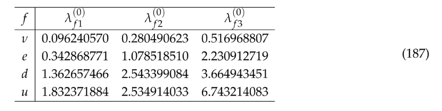
A higher-precision signed choice of the real orthogonal overlap representatives is
,
. The signs of individual real eigenvectors are conventional. Row or column sign changes therefore modify a representative without changing its entrywise moduli, rephasing-equivalence class, closed-cycle invariants, or the principal angles of the corresponding spectral subspaces.
D. Orthogonal Sector-Character Decomposition
The orthogonal transform in Equation (169) reorganizes the four sector labels into one average component and three independent contrasts. Applied to the evaluated canonical family operators in the common frame , it gives
The inverse character transform reproduces all four sector matrices with relative Frobenius defect . The norm-square fractions in Equation (170) are computed as
Because is orthogonal in sector-label coefficient space, the transformation is invertible and preserves the summed Frobenius norm. It is therefore an exact decomposition of the evaluated four-sector tuple, not the addition of new operators. The symbols label algebraic contrasts only; a microscopic weak, color, or mixed interpretation requires the corresponding symmetry action and is not supplied by the transform alone.
E. Finite-Dimensional Feshbach Realization
The following finite-dimensional realization verifies the algebraic equivalence between the full block eigenvalue problem and its reduced Schur–Feshbach equation. Take
and form
For the reduced equation
the unique root in and the lowest eigenvalue of are both . The scalar residual is and the relative eigenvalue defect is zero at the recorded precision. This is a concrete check of the identity used in Equation (150); the general result follows from the block factorization in Equation (17). The example verifies the reduction method and is not a model of a physical fermion self-energy.
F. Static Obstruction and Perturbation Calculations
The numerical evaluation separates the candidate data from the observational comparisons. The family arrays determine spectra and overlaps, the declared dimensionful representation determines the conservative mass scale, and empirical constants enter only when the invariant candidate outputs are tested. The calculation performs:
- (i)
- all 36 row/column permutations of against the PDG CKM central matrix;
- (ii)
- the minimum possible electron-row entry of under neutrino-column permutations;
- (iii)
- the rest-energy ratios and the electron-anchored RMS ratio ;
- (iv)
- the conservative charged-lepton mass ratios, same-label energy differences, and relabeling-independent total pole-correction lower bounds in the fixed decomposition;
- (v)
- the Weyl–Davis–Kahan robust-neighborhood numerical results, including the uniform radius, diagnostic-specific radii, the dimensionless relative radius, and the joint operator–metric perturbation corollary.
The best CKM permutation has Frobenius mismatch , the smallest static electron-row element is , the rest-energy endpoint ratios are , and . Together with the analytic bounds in Theorem 8.4 and Corollary 8.5, these values show that the full spectral-norm ball of radius around the canonical tuple remains outside the broad regions in Equation (120). The endpoint obstruction is the electron-anchored kinematic statement for the displayed active-neutrino assignment. The KATRIN ratio is retained only as a scale diagnostic and is not counted as a second independent exclusion.
G. Numerical Inputs and Reproducibility
The Supplement contains the machine-readable objects needed to reproduce the finite-dimensional calculations: the rank-six quotient and seven action-block Hessians; the stationary Schur reduction; the action-normal and BKM-normal operators; the two equivalent scale factorizations; the common family metric and four sector forms; the signed overlap representatives; and the arrays used in the perturbation-neighborhood and finite-dimensional Feshbach calculations. File identifiers, array keys, software requirements, and integrity checks are kept in the Supplement so that the main text can remain focused on the physical argument.
The numerical programs recompute the spectra, overlaps, obstruction diagnostics, factorization identities, and finite-dimensional consistency relations from the supplied arrays. The candidate operators remain fixed throughout these calculations, while observational quantities enter only in the final comparison functions. Reproduction of these finite-dimensional results establishes the stated arithmetic and operator calculations; it is distinct from a microscopic derivation of the candidate data from the parent fields.
References
- D. Lee, The 11D–4D Covariant Master Equation for a Unified Field Theory, Version 5.0, Zenodo (2026), published July 13, 2026. [CrossRef]
- Higgs, P. W. Broken Symmetries and the Masses of Gauge Bosons. Phys. Rev. Lett. 1964, 13, 508–509. [Google Scholar] [CrossRef]
- Weinberg, S. A Model of Leptons. Phys. Rev. Lett. 1967, 19, 1264–1266. [Google Scholar] [CrossRef]
- Weinberg, S. Baryon- and Lepton-Nonconserving Processes. Phys. Rev. Lett. 1979, 43, 1566–1570. [Google Scholar] [CrossRef]
- Chamseddine, A. H.; Connes, A. The Spectral Action Principle. Commun. Math. Phys. 1997, 186, 731–750. [Google Scholar] [CrossRef]
- Chamseddine, A. H.; Connes, A.; Marcolli, M. Gravity and the Standard Model with Neutrino Mixing. Adv. Theor. Math. Phys. 2007, 11, 991–1089. [Google Scholar] [CrossRef]
- Dąbrowski, L.; Sitarz, A. Fermion Masses, Mass-Mixing and the Almost Commutative Geometry of the Standard Model. J. High Energy Phys. 2019, 02, 068. [Google Scholar] [CrossRef]
- Roberts, C. D.; Williams, A. G. Dyson–Schwinger Equations and Their Application to Hadronic Physics. Prog. Part. Nucl. Phys. 1994, 33, 477–575. [Google Scholar] [CrossRef]
- Pilaftsis, A. Resonant CP Violation Induced by Particle Mixing in Transition Amplitudes. Nucl. Phys. B 1997, 504, 61–107. [Google Scholar] [CrossRef]
- Cabibbo, N. Unitary Symmetry and Leptonic Decays. Phys. Rev. Lett. 1963, 10, 531–533. [Google Scholar] [CrossRef]
- Kobayashi, M.; Maskawa, T. CP-Violation in the Renormalizable Theory of Weak Interaction. Prog. Theor. Phys. 1973, 49, 652–657. [Google Scholar] [CrossRef]
- Maki, Z.; Nakagawa, M.; Sakata, S. Remarks on the Unified Model of Elementary Particles. Prog. Theor. Phys. 1962, 28, 870–880. [Google Scholar] [CrossRef]
- Feshbach, H. Unified Theory of Nuclear Reactions. Ann. Phys. (N.Y.) 1958, 5, 357–390. [Google Scholar] [CrossRef]
- Feshbach, H. A Unified Theory of Nuclear Reactions. II. Ann. Phys. (N.Y.) 1962, 19, 287–313. [Google Scholar] [CrossRef]
- Källén, G. On the Definition of the Renormalization Constants in Quantum Electrodynamics. Helv. Phys. Acta 1952, 25, 417–434. [Google Scholar]
- Lehmann, H. Über Eigenschaften von Ausbreitungsfunktionen und Renormierungskonstanten quantisierter Felder. Nuovo Cim. 1954, 11, 342–357. [Google Scholar] [CrossRef]
- Gesztesy, F.; Tsekanovskii, E. On Matrix-Valued Herglotz Functions. Math. Nachr. 2000, arXiv:funct218, 61–138. [Google Scholar] [CrossRef]
- Dusson, G.; Sigal, I. M.; Stamm, B. “The Feshbach–Schur Map and Perturbation Theory,” in Partial Differential Equations, Spectral Theory, and Mathematical Physics. EMS Ser. Congr. Rep. 2021, 18, 65–88. [Google Scholar] [CrossRef]
- T. Kato, Perturbation Theory for Linear Operators, 2nd ed. (Springer, Berlin, 1995). 2nd ed. [CrossRef]
- R. Bhatia, Positive Definite Matrices (Princeton University Press, Princeton, 2007).
- R. A. Horn and C. R. Johnson, Matrix Analysis, 2nd ed. (Cambridge University Press, Cambridge, 2013),. [CrossRef]
- Buckingham, E. On Physically Similar Systems; Illustrations of the Use of Dimensional Equations. Phys. Rev. 1914, 4, 345–376. [Google Scholar] [CrossRef]
- Kubo, R. Statistical-Mechanical Theory of Irreversible Processes. I. J. Phys. Soc. Jpn. 1957, 12, 570–586. [Google Scholar] [CrossRef]
- Petz, D. Monotone Metrics on Matrix Spaces. Linear Algebra Appl. 1996, 244, 81–96. [Google Scholar] [CrossRef]
- Unruh, W. G. Notes on Black-Hole Evaporation. Phys. Rev. D. 1976, 14, 870–892. [Google Scholar] [CrossRef]
- Rotter, I. A Non-Hermitian Hamilton Operator and the Physics of Open Quantum Systems. J. Phys. A Math. Theor. 2009, 42, 153001. [Google Scholar] [CrossRef]
- Takahashi, F.; et al. (Particle Data Group), Review of Particle Physics. Int. J. Mod. Phys. A 2026, 41, 2630011. [Google Scholar] [CrossRef]
- Mohr, P. J.; Newell, D. B.; Taylor, B. N.; Tiesinga, E. CODATA Recommended Values of the Fundamental Physical Constants: 2022. Rev. Mod. Phys. 2025, 97, 025002. [Google Scholar] [CrossRef]
- N. Aghanim et al. (Planck Collaboration) Planck 2018 Results. VI. Cosmological Parameters. Astron. Astrophys. 2020, 641, A6. [Google Scholar] [CrossRef]
- Beneke, M. Pole Mass Renormalon and Its Ramifications. Eur. Phys. J. Spec. Top. 2021, 230, 2565–2579. [Google Scholar] [CrossRef]
- H. Georgi, Lie Algebras in Particle Physics, 2nd ed. (Westview Press, Boulder, 1999). 2nd ed.
- Kniehl, B. A. All-Order Renormalization of the Propagator Matrix for Fermionic Systems with Flavor Mixing. Phys. Rev. Lett. 2014, 112, 071603. [Google Scholar] [CrossRef]
- Kniehl, B. A. Propagator Mixing Renormalization for Majorana Fermions. Phys. Rev. D. 2014, 89, 116010. [Google Scholar] [CrossRef]
- Buchholz, D. Gauss’ Law and the Infraparticle Problem. Phys. Lett. B 1986, 174, 331–334. [Google Scholar] [CrossRef]
- M. Aker et al. (KATRIN Collaboration) Direct Neutrino-Mass Measurement Based on 259 Days of KATRIN Data. Science 2025, 388, 180–185. [Google Scholar] [CrossRef]
- M. C. Delfour and J.-P. Zolésio, Shapes and Geometries: Metrics, Analysis, Differential Calculus, and Optimization, 2nd ed. (SIAM, Philadelphia, 2011),. [CrossRef]
- Davis, C.; Kahan, W. M. The Rotation of Eigenvectors by a Perturbation. III. SIAM J. Numer. Anal. 1970, 7, 1–46. [Google Scholar] [CrossRef]
- G. W. Stewart and J.-G. Sun, Matrix Perturbation Theory (Academic Press, Boston, 1990).
- H. M. Nussenzveig, Causality and Dispersion Relations (Academic Press, New York, 1972).
- D. Lee, “A First-Principles Derivation of Absolute Physical Scale from an Eleven-Dimensional Covariant Master Action,” Zenodo, Version 2.0 (2026), published October 3, 2026. 3 October. [CrossRef]
Table 1.
Physical role of the inputs entering the reduced operator problem.
| Input | Role in the analysis |
| , , and | Conservative scale–family geometry of the specified finite-dimensional branch. |
| Dimensionful realization of the common conservative scale. | |
| , , , and | Open-complement data defining the reduced retarded pencil and its analytic branch. |
| Masses, mixing matrices, and endpoint data | External diagnostics applied to the invariant spectra and subspaces after the operator tuple has been fixed. |
Table 3.
Conservative four-sector spectrum of the specified finite-dimensional candidate. The labels are ordered eigenmodes of the printed family operators, not prior identifications with the observed pole generations.
Table 3.
Conservative four-sector spectrum of the specified finite-dimensional candidate. The labels are ordered eigenmodes of the printed family operators, not prior identifications with the observed pole generations.
| Mode | Mass (kg) | Mass (MeV/) | |
| 2.311760529 | 1.181307203 | ||
| 2.719052872 | 1.389433163 | ||
| 4.434753740 | 2.266154505 | ||
| 1.993560338 | 1.018707239 | ||
| 2.723599777 | 1.391756626 | ||
| 3.269412161 | 1.670666181 | ||
| 1 | 0.510998950 | ||
| 1.773576135 | 0.906295543 | ||
| 2.550805381 | 1.303458871 | ||
| 0.529803872 | 0.270729222 | ||
| 0.904472170 | 0.462184329 | ||
| 1.227914716 | 0.627463131 |
Table 4.
Critical numerically evaluated radii for the broad diagnostics. Strict exclusion holds for ; equality is the contact value at which the corresponding bound first reaches the enlarged acceptance boundary. The uniform theorem uses the smaller common radius , and the PMNS entry is the limiting condition.
| Diagnostic acceptance condition | Critical radius |
| Electron-anchored endpoint |
Disclaimer/Publisher’s Note: The statements, opinions and data contained in all publications are solely those of the individual author(s) and contributor(s) and not of MDPI and/or the editor(s). MDPI and/or the editor(s) disclaim responsibility for any injury to people or property resulting from any ideas, methods, instructions or products referred to in the content. |
© 2026 by the authors. Licensee MDPI, Basel, Switzerland. This article is an open access article distributed under the terms and conditions of the Creative Commons Attribution (CC BY) license (http://creativecommons.org/licenses/by/4.0/).
Copyright: This open access article is published under a Creative Commons CC BY 4.0 license, which permit the free download, distribution, and reuse, provided that the author and preprint are cited in any reuse.