

Submitted:
11 October 2026
Posted:
12 October 2026
You are already at the latest version
Abstract
Space debris fragments too small to track can still reach speeds capable of disabling a spacecraft. The number of such fragments remains uncertain, making it difficult to assess risks to satellites supporting Earth-critical services such as broadband and GPS. We combine radar detection with a Bayesian model to adaptively choose where a radar should point next, aiming to reduce uncertainty. We analyzed about 24 hours of data from each of the two European Incoherent Scatter Scientific Association (EISCAT) radars: the Tromsø ultra high frequency radar and the EISCAT Svalbard radar. We first used a Generalized Matched Filter to search for radar signals consistent with moving objects. Tests with 4,000 simulated object signals in raw voltage data led us to select cell-averaging Constant False Alarm Rate (CA-CFAR) detection. For external validation on another radar, we applied the CA-CFAR detector selected using the Tromsø recordings to the Svalbard recordings without retuning. The method found 155 events at Tromsø and 222 at Svalbard. Of these, 106 and 119, respectively, could not be confidently matched to cataloged objects. We used the Tromsø rate of unresolved events to calibrate a Bayesian population model informed by the Orbital Debris Engineering Model (ORDEM). With this model, we compared radar pointing schedules across 300 simulated worlds, giving each schedule 24 observations. Adaptive pointing with service weights reduced uncertainty at the final observation by 41.2%, 15.4%, and 5.35% relative to fixed, random, and preplanned schedules, respectively. The additional improvement over unweighted adaptive pointing was estimated at 1.55% (95% interval: -0.47% to 3.53%), a small difference that was not statistically significant. The simulations provide strong evidence that adaptive pointing can reduce uncertainty around hidden debris using the same number of observations, potentially improving the information used to assess risks to important satellite services.
Keywords:
space debris
; radar detection
; Bayesian inference
; adaptive sensor tasking
; service-aware scheduling
; EISCAT
1. Introduction
The European Space Agency (ESA) estimates that about 1.5 million debris objects between 1 and 10 cm are in orbit [1]. Most cannot be followed individually, but a collision with one can still damage or disable a spacecraft. This makes it difficult to assess the risk posed by debris whose orbits are unknown. Kessler and Cour-Palais showed that collisions can create fragments that make later collisions more likely [2]. Later studies examined how traffic, disposal, and mitigation affect the debris environment [3,4].
In this paper, we use the term hidden debris to describe debris that lacks a reliable orbital record in public catalogs. Many small fragments have no public orbital record, and records for larger debris can also be missing or out of date.
The National Aeronautics and Space Administration (NASA) developed the Orbital Debris Engineering Model (ORDEM), while ESA developed the Meteoroid and Space Debris Terrestrial Environment Reference (MASTER) [5,6,7,8]. These models combine measurements with assumptions about debris sources to estimate debris populations that cannot be counted individually. Their estimates can differ, especially for smaller debris [7,8].
In a beam park observation, the radar points in one direction. As debris orbits Earth, some pieces pass through the radar beam and can be detected without knowing their orbits in advance. In January 2018, the European Incoherent Scatter Scientific Association (EISCAT) collected simultaneous observations with its Tromsø ultra high frequency radar and the EISCAT Svalbard Radar [9]. We selected the detection settings using the Tromsø recordings, grouped detections into radar events, and checked whether those events matched cataloged objects. We then applied the selected detector without retuning to all usable Svalbard recordings as a test on a second radar.
However, the EISCAT radars kept fixed pointing directions during the campaign, which raises a second question: if a radar were able to choose where to observe next, could it learn the debris population more efficiently? Previous sensor tasking research has already shown that observation schedules can be changed according to uncertainty, information gain, or the need to monitor known objects [10,11,12,13,14,15]. Much of this work focuses on individual objects with known orbits. Our study instead asks whether adaptive observations can improve knowledge of a hidden debris population.
We test adaptive pointing in simulation using Bayesian experimental design. The model estimates the hidden debris population and how uncertain that estimate is. Before each new observation, it compares possible pointing directions and chooses the one expected to reduce uncertainty the most [16,17,18]. We also test whether giving more weight to altitudes occupied by satellites supporting critical infrastructure reduces uncertainty further.
Accordingly, the paper evaluates three linked questions:
- How well does the cell averaging constant false alarm rate (CA-CFAR) detector selected using Tromsø UHF radar beam park recordings perform on EISCAT Svalbard Radar beam park recordings without retuning?
- Under the same observation budget, how much and how quickly does adaptive elevation selection reduce uncertainty compared with fixed, random, and preplanned schedules?
- Does adding service weights to adaptive elevation selection reduce uncertainty more than unweighted adaptation?
Section 2 of this paper reviews previous work on debris models, beam park radar, catalog association, adaptive observation, and service weights. Section 3 describes the radar analysis, Bayesian population model, and scheduling simulation. Section 4 presents the radar results and compares the simulated schedules. Section 5 discusses the findings and limitations, and Section 6 concludes.
2. Literature Review
2.1. Debris Environment Models and Observational Limits
Catalogs help researchers follow individual objects, but they cannot describe all the debris in orbit. Smaller fragments are usually estimated statistically, and even larger objects can be difficult to identify when their orbital records become outdated or go missing. Early research examined how debris is produced and how its numbers might grow, including the possibility that collisions could create more fragments [2,19,20]. Later models examined how launches, explosions, collisions, atmospheric drag, disposal, and mitigation affect the population over time [4,21,22,23,24].
MASTER and ORDEM were developed to estimate debris that cannot be followed one object at a time. MASTER models how several debris sources are produced and estimates their distributions through orbital space, while ORDEM combines measurements with modeled populations to estimate the debris that spacecraft may encounter [5,6]. Studies of collisions show that these estimates depend partly on assumptions about how many fragments a breakup produces and how those fragments move over time [25,26]. They also depend on which debris sources a model includes. For example, Bendisch et al. extended MASTER to include particles from solid rocket motors, material shed from spacecraft surfaces, and coolant droplets released by nuclear-powered satellites [27].
Comparisons among these models show that their estimates can differ. Krisko et al. reported differences between ORDEM 3.0 and MASTER-2009 and found differences in predicted debris flux across many orbits [7]. Liu et al. compared the Space Debris Environment Engineering Model (SDEEM) with ORDEM and found that much of the difference came from how they estimated debris missing from catalogs [8]. These comparisons show that estimates of uncataloged debris depend on the assumptions built into each model.
2.2. Beam Park Radar Sampling and Population Estimation
Beam park surveys provide measurements of debris that public catalogs often miss. The radar points in a fixed direction as objects pass through its beam. The number detected depends on the debris population, but also on the radar’s sensitivity, the ranges it measures, and where it points.
Early surveys with the MU, Haystack, Goldstone, and TIRA radars demonstrated that this approach could observe small debris and compare detection rates with model predictions [28,29,30,31,32]. Haystack studies also showed that the viewing geometry affects the debris observed [33]. TIRA used both fixed beam surveys and observations that followed individual objects [34]. At Goldstone, a later change to the receiving antenna narrowed the range that could be observed at one time [35]. Raw detection counts from different radars therefore cannot be compared without considering how each instrument collected its data.
EISCAT offers another example. Its radars were built primarily for ionospheric research, but researchers also used them to observe debris [36]. Landgraf et al. compared early EISCAT measurements with MASTER. They found that the observed altitude distribution agreed with the model more closely than the estimated object sizes did, partly because the location of an object within the radar beam was unknown [37]. Markkanen et al. later studied how to process EISCAT debris signals in real time [38]. In January 2018, Vierinen et al. used the Tromsø and Svalbard radars simultaneously. Their analysis searched over range, radial velocity, and acceleration, then compared the detections with a catalog and with MASTER [9].
A radar return also does not reveal an object’s diameter directly. Radar cross section describes how strongly it reflects the transmitted signal, and that strength changes with the object’s material, shape, and orientation [39]. Near the detection limit, a weak return may be missed altogether [40]. These effects matter when an event count is used to estimate how much debris exists at a given size.
Estimating a population from beam park data requires a model of how often objects with different sizes and orbits would pass through the beam and be detected. Earlier work estimated population uncertainty from such observations [41]. Vierinen et al. later used prior information and a model of expected radar detections to estimate debris density [42]. These studies show how to infer a population from the directions already observed. They leave open the question of which direction would be most informative to observe next.
2.3. Detection, Fluctuating Targets, and Catalog Association
In beam park observations, weak echoes from small objects can be hidden by noise. A matched filter uses the known pattern of the transmitted radar pulse to search for an echo in the received signal. The generalized matched filter (GMF) also accounts for an object’s motion while several pulses are collected. It searches over possible ranges, radial velocities, and accelerations so that weak returns from the same moving object can be added together [9]. A peak in the GMF output is a possible detection, although noise, interference, and antenna sidelobes can also produce peaks.
The next decision is how large a peak must be before it counts as a detection. A low threshold finds more faint echoes but also produces more false alarms. A high threshold rejects more noise but misses some weak objects. Radar operating curves describe this relationship through the probabilities of detection and false alarm at a given signal-to-noise ratio [43,44]. A fixed threshold uses the same cutoff throughout the data. Constant false alarm rate (CFAR) methods adjust the cutoff using nearby measurements of the background. Rohling showed that a simple average of those measurements can be misleading when they include another strong echo or cross a sharp change in the background [45]. Later CFAR methods examined other ways to handle these conditions [46,47].
As a debris fragment travels along its orbit, it may also tumble. The surface facing the radar can change, making its echo stronger or weaker even when the fragment follows the same orbital path. Swerling’s four cases describe different patterns of change in radar cross section [43]. In cases I and III, the cross section stays roughly constant over the pulses in one radar scan and changes between scans. In cases II and IV, it changes from pulse to pulse. The cases also differ in how widely the echo strength varies. Cases I and II have larger fluctuations, associated with several reflecting parts of similar strength. Cases III and IV have smaller fluctuations, associated with one reflecting part that dominates the return. This variation affects which pieces of debris the radar detects, even among objects that pass through its beam.
The next step after detection is to see whether a cataloged object could have produced the radar event. Simplified General Perturbations 4 (SGP4) uses two-line element (TLE) sets to predict where cataloged objects should be at the observation time [48]. Those predictions depend on how accurate and current the records are. An object crosses the fixed radar beam in a short time, leaving only a brief set of measurements to compare with the predictions. More than one cataloged object may fit those measurements, so a match can remain uncertain [49,50]. We classify events without a confident match as unresolved, since a failed match alone does not show that a new debris object has been found.
2.4. Adaptive Radar and Sensor Scheduling
The beam park studies discussed above kept the radar pointed in one direction while debris passed through the beam [9,42]. A radar that can change elevation could use what it has measured so far to decide where to look next. This choice matters when observation time is limited and some altitudes remain poorly measured.
The broader problem is how to spend limited observation time when the answer is uncertain. In optimal search theory, Stone et al. account for where a target might be, the chance that a sensor will miss it, and the effort available to search [51]. Zhao et al. examined how sensors working together could choose measurements that provide useful information without excessive communication or computing costs [52]. Julian et al. took the idea further for mobile robots, moving their sensors as they learned about an environment [53]. Their goal was to improve an estimate spread over space, which is closer to learning a debris population than locating one known object.
In space surveillance, the next observation is often chosen to improve a known object’s orbit. As time passes without another measurement, its predicted position becomes less certain. Researchers have used that uncertainty, expected information gain, and plans for future observations to decide where a sensor should look [10,12,54,55]. A radar also needs time to search for objects missing from the catalog. Moretti et al. compared a step scan with dynamic tasking, while Cai et al. studied how to divide observing time between searches and repeat observations of known geosynchronous objects [11,13]. Siew et al. used reinforcement learning to schedule ground and space sensors, assessing how many objects were observed and how much their orbital estimates improved [14,15]. In these studies, the schedule is judged mainly by how well it finds or follows individual objects [56]. A brief radar detection may never yield an orbit reliable enough to follow, but it can still provide evidence about debris abundance.
Scheduling several sensors also adds practical constraints. Each sensor has its own viewing opportunities, and different objects may need attention at the same time. Studies of surveillance networks have addressed how to allocate observations under such conditions [57,58,59]. Xue et al. review the wider range of methods used for space surveillance scheduling [60]. Our simulation focuses on the choice of elevation for one radar. After each observation, it selects the elevation expected to reduce uncertainty about debris abundance across altitude. We compare the resulting estimates with fixed, random, and preplanned schedules under the same observation budget.
2.5. Bayesian Experimental Design
Choosing a radar direction using earlier measurements is a version of a much older problem in statistics. Chaloner studied how uncertainty and the purpose of an experiment affect which measurements are worth taking. Her later review with Verdinelli described Bayesian experimental design more broadly as a decision made before the results are known [16,17]. Possible results must be considered when estimating the value of an observation. For large or nonlinear models, that calculation can become difficult, and making it practical remains an active area of research [61,62].
At an elevation that has already been measured well, more detections may add less information than a smaller number from a poorly measured altitude. Information gain considers how much an observation is expected to change what is currently known. Oladyshkin and Nowak examined its connection to Bayesian updating, while Kleinegesse et al. studied how to choose observations when a model can simulate measurements but cannot easily calculate their probabilities [63,64]. The answer also depends on what researchers want to estimate. Attia et al. considered designs that improve a particular quantity rather than every model parameter, and later work extended this approach to more complicated quantities [18,65,66]. Different goals can favor different observations.
A schedule can visit several elevations without changing its plan when new data arrive. Joshi and Boyd studied how to choose an informative set of sensors in advance. Nemhauser et al. showed that, under certain conditions, selecting one useful measurement at a time can produce a strong set [67,68]. These results do not directly predict how a debris radar will perform. They do show why a planned schedule using several directions is a more demanding comparison for adaptive pointing than holding the radar at one elevation.
The number of radar events depends on both the debris population and the chance that passing objects are detected. If fewer events appear than expected, either part of that explanation could be wrong. Kennedy and O’Hagan studied how to calibrate models against measurements, and Brynjarsdóttir and O’Hagan showed that overlooking errors in a model can produce biased and overly confident estimates [69,70]. Bartuska et al. studied how uncertainty in factors that affect measurements complicates experimental design [71,72]. Cademartori examined the related problem of whether the available data can distinguish different unknowns [73]. Uncertainty about the radar response can therefore change which elevation appears most useful.
2.6. Debris Prioritization and Satellite Services
A breakup near operating satellites can create fragments that threaten other spacecraft later. Studies of collisions and debris growth have examined how that danger depends on where a breakup occurs [74,75,76]. Other work has ranked large objects by how much new debris they could produce if they break apart [77,78]. These studies help identify regions where future debris growth is a concern. Deciding where better measurements are needed also calls for looking at the satellites already in those regions and the services they provide.
Rao et al. studied how debris and crowded orbits create costs for satellite operators [79]. Xu et al. modeled how losing particular satellites affects the rest of a network [80]. C-SWIM examined a different hazard, solar particle radiation, and grouped satellites by five services: navigation, communications, weather, Earth observation, and military or intelligence [81]. Knowing where satellites providing these services operate can help prioritize altitudes where better estimates of the debris population would be valuable.
Earlier beam park work estimated debris populations from fixed observations, while adaptive sensor studies have mainly focused on objects that can be followed individually. The literature leaves open whether a radar can reduce uncertainty about debris it cannot track by changing elevation as observations arrive, and whether service information helps it use a limited observation budget more effectively.
3. Methodology
Figure 1.
Complete methodological outline of the research
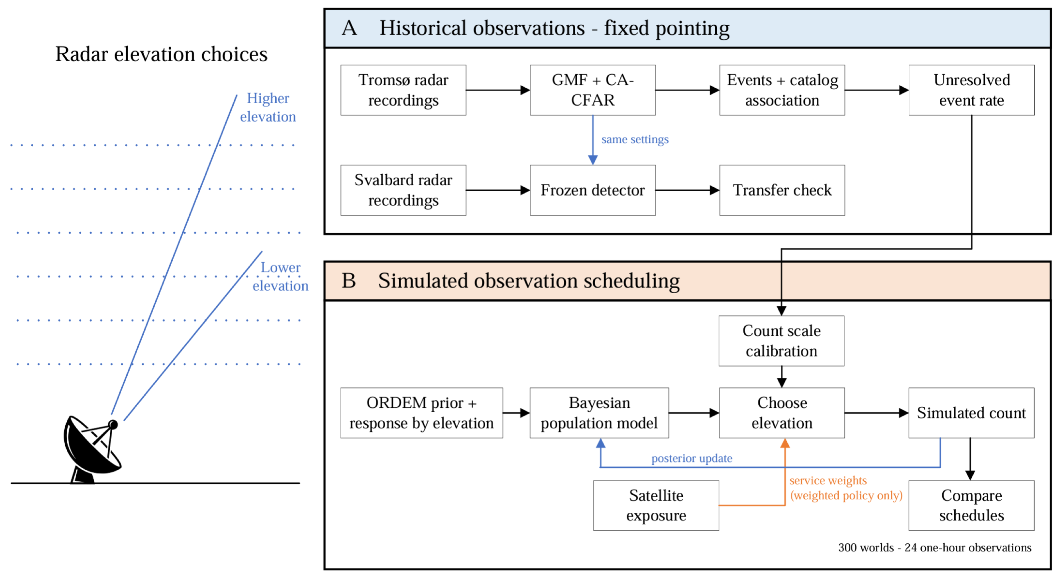
3.1. Study Design
We analyzed EISCAT radar data collected on January 4 and 5, 2018. The Tromsø record covers the 24 hours beginning at 12:00 UTC on January 4. The radar pointed at an azimuth of and an elevation of , and we analyzed returns at slant ranges between 1,026.639 and 1,084.050 km. The Tromsø radar operated at 930 MHz, while the Svalbard radar operated at 500 MHz. Both recorded voltage samples during simultaneous beam park observations [9]. We used these data to choose the detector, group detections into events, and check which events matched cataloged objects. We then ran the detector on the Svalbard data without changing its settings to see how well it worked on a second radar.
The Tromsø events without confident catalog matches provided the count rate used to calibrate the debris population model. Neither radar changed direction during the campaign, so we used simulation to study what could be learned by changing elevation. After each simulated observation, the model updated its estimate of debris abundance by altitude, and the adaptive scheduler chose where to point next. We compared adaptive schedules with and without service weights against fixed, random, and preplanned schedules. Each schedule received 24 observations lasting one hour each in each of 300 simulated worlds.
3.2. GMF Processing
The original EISCAT recordings were stored as MATLAB data files (.mat), containing the sampled radar signals and measurement information. We converted them to Digital RF, a format that stores radio signals in time order, and processed them with Hardtarget, which implements the generalized matched filter (GMF). Every hour was processed with the same settings and software revision.1
The GMF searched the radar data for signals consistent with moving objects. It compared the measurements with signals expected at different ranges, radial speeds, and accelerations. Ten radar pulses were combined for each coherent measurement, giving one processed time step every 0.2 seconds. The GMF produced a score over time and range. A high score meant that the data were consistent with a moving target, but noise, interference, or a brief change in the background could also produce a peak. We counted a radar event only when nearby responses formed a consistent path through time.
3.3. Detector Calibration
We compared a fixed signal-to-noise ratio (SNR) threshold with two methods that set their cutoff using nearby GMF scores: cell averaging CFAR (CA-CFAR) and ordered statistics CFAR (OS-CFAR). For each range cell being tested, the CFAR methods skipped the nearest 16 cells on either side, then used the next 32 cells on each side to estimate the background. CA-CFAR used the mean of these 64 values. OS-CFAR sorted them and used the 48th lowest [45]. All three methods ignored the outer 48 cells at each end of the range window and kept only peaks that were highest among three neighboring range cells.
We tested every setting with the same 4,000 artificial echoes, generated in simulated raw radar voltage before GMF processing. Eight hundred had steady strength, and 800 followed each of the four Swerling models [43]. An echo counted as recovered only if it passed through the full processing pipeline. We compared recovery by echo strength, duration, and Swerling model, and calculated 95% Wilson intervals for the recovery fractions.
We also tested the pipeline on shuffled versions of the real Tromsø data. We cut the GMF measurements into 0.4 second blocks, shuffled the blocks, and ran the data through detection and grouping again. Shuffling kept brief features of the measured signal but broke up the longer pattern made by an object passing through the beam. We counted how many detections the pipeline still reported after grouping. If it reported k detections over E hours of shuffled data, the rate per 24 hours was . Because a small count gives an uncertain rate, we also calculated an exact one-sided 95% Poisson upper bound. The shuffles reused the same Tromsø measurements, so these rates cannot establish how often false detections would occur on a new day of observation.
We used the shuffled Tromsø data to help choose the detector. We set a limit of one event per 24 hours for the 95% upper estimate and excluded any setting above it. One event per day was a practical limit chosen for this study, not a radar standard. Among the remaining settings, we chose the one that recovered the most short, faint echoes under Swerling models I, II, III, and IV. For this comparison, the echoes lasted at most 2 seconds and had an output SNR of at most 14 dB if their strength stayed steady. If settings tied, we favored higher recovery for the Swerling model with the lowest recovery, then higher recovery across all four models, and finally the lower upper bound.
We repeated the selection six times, leaving out a different four hour section of Tromsø data each time to see whether the choice changed. Using all the Tromsø data, we selected CA-CFAR with a threshold of 1.75 times the local mean. We used the same setting on Svalbard.
3.4. Event Construction and Catalog Association
One object can appear in the radar data at several consecutive times. We linked detections that followed a consistent change in distance from the radar, keeping the strongest response every 0.2 seconds. We accepted a group if it contained at least five measurements spanning 0.8 seconds, its fitted range had a root mean square error no greater than 0.45 km, and its radial speed was no greater than 6 km/s. If an echo faded briefly, one passage could be split into two groups. We combined two groups if the gap between them was no more than 7 seconds or they overlapped by no more than 0.4 seconds. Using each group’s measured motion, we estimated its distance from the radar at the time halfway between the middle times of the two groups. These distances had to agree within 0.75 km, and their radial speeds had to agree within 0.15 km/s.
We then checked whether a cataloged object could explain each radar event. SGP4 used the latest TLE set available before the observation to predict each object’s range and radial speed at the event time [48]. The object had to be visible from the radar and within of its pointing direction. Its predicted range had to agree with the measurement within the larger of 1 km or 0.1% of the measured range. For radial speed, the limit was the larger of 0.020 km/s or 1% of the measured speed. We assigned a catalog identity only when exactly one object met all these conditions.
For Tromsø events without a match, we made a second comparison based on the differences seen in confident matches. This allowed range differences up to 3 km and radial speed differences up to 0.060 km/s. We compared each cataloged object’s predicted range and radial speed with the radar measurements. Using the differences seen in the main matches as a reference, we combined these differences into one score called the squared Mahalanobis distance (). A lower score meant a closer fit. Exactly one object had to meet the range, speed, and viewing limits and have , the 99% acceptance cutoff. If several objects met the viewing limits, the best score had to be at least 4.0 lower than the next best score. The radar event also had to last at least 5 seconds or have a peak detector score of at least 30. We also shifted the catalog predictions forward and backward by 15 and 30 minutes to check how often similar matches occurred by chance. The additional matches were kept only if those shifts produced, on average, at most one tenth as many matches. We did not use this second comparison for Svalbard. Events without a confident match were classified as unresolved.
3.5. Bayesian Population and Response Model
We divided the altitude range from 915 to 1,065 km into ten bands, each 15 km wide. In the simulation, the radar could choose among 49 elevations from to in steps, with azimuth held at .
For each band j, the model estimated a multiplier relative to the ORDEM population estimate. A value of keeps the ORDEM baseline, while 2 doubles it and 0.5 halves it. The multiplier describes a relative change in the modeled population, not a direct count of objects.
Changing elevation changes which altitudes contribute to a radar observation. We used to describe the modeled contribution of band j when the radar points at elevation a. One elevation can receive contributions from several bands, and nearby elevations often sample much of the same altitude range. The main analysis used the ORDEM population larger than 1 cm to construct this response table. We used ORDEM 3.2.0 predictions for 2018. We summed the flux contributions from its five debris groups, weighted each range interval by its overlap with the analyzed slant range window, and grouped the contributions into the ten altitude bands.
For a simulated one-hour observation t at elevation , we modeled the expected number of unresolved events as
The sum combines the contributions from the ten altitude bands. The scale s converts the ORDEM response into an hourly event count, while allows the response at the chosen elevation to differ from its modeled value. A value of represents the nominal response. We set the background allowance b to about 0.041 events per hour using the shuffled controls described above. For those controls, we rearranged blocks of real radar measurements to disrupt the continuous signal from a passing object, then checked how often the processing still produced an event. The value used for b was the 95% upper rate from that test.
The count in any one hour does not need to equal . We represented this variation with a negative binomial model for the simulated count , using :
We obtained from the variation in the 24 hourly totals of accepted Tromsø events, using the fifth percentile of estimates from resampled hourly counts. We then applied it to the simulated unresolved counts. The second term in the equation allows more variation between hours than a Poisson model, whose variance would equal its mean.
The Tromsø data also set the count scale s. There were 106 unresolved events in 24 hours at the historical pointing direction. After allowing for b, we divided that hourly rate by the total response predicted at when all and the response factor equal one:
When all the multipliers equal one, the model predicts the average event rate measured at Tromsø’s elevation. Tromsø did not observe the other elevations, so their predicted rates come from ORDEM. The 106 unresolved events set the scale of these predictions; they are not a count of uncataloged objects, since some could be missed catalog matches or false detections.
The model allows two things to vary. The population multiplier changes the assumed amount of debris in altitude band j. The response factor changes how strongly the radar is expected to respond at elevation a. We modeled their logarithms so both factors stay positive. For the population, the prior had a log standard deviation of 0.6537 and a median multiplier of one. We used a Matérn kernel to allow population values in nearby altitude bands to vary together over a 30 km scale, with 25% of the variation independent between bands. For the radar response, uncertainty came from the saved response estimates, and the response factors had a prior mean of one. We used a squared exponential kernel to allow responses at nearby elevations to vary together over a scale, with 10% independent variation. A low event count could therefore mean less debris, a weaker response, or both.
3.6. Posterior Estimation
Each simulated hour produced a count of unresolved events. We used that count and all earlier counts to update which debris populations and radar responses remained plausible. This updated picture is called the posterior. It combines the starting assumptions (the prior) with how well each possible set of values explains the observed counts (the likelihood):
The update involved the ten population multipliers and 49 radar response factors introduced above. We transformed them using their prior uncertainty and how they varied together, which made the numerical fitting more stable. After finding the values where the posterior was highest, we estimated how much the values could vary and still fit the data. We did this from the shape of the posterior near its highest point, a method called the Laplace approximation. It was fast enough to repeat after every observation. We then converted the uncertainty back to the population multiplier scale and recorded it in . The diagonal of this matrix gives the variance for each altitude band.
After each 24-observation simulation ended, we made a more detailed check by drawing values from the posterior using elliptical slice sampling. We did this for all 300 simulated worlds under each of the five schedules: fixed, random, preplanned, adaptive without service weights, and adaptive with service weights. For each final estimate, we ran the sampling method four separate times. We extended the runs until they gave similar results () and provided enough useful samples from both the center and the extremes of the posterior (bulk and tail effective sample sizes of at least 400).
These samples supplied the final comparisons of remaining uncertainty, error in the estimated populations, and how often the uncertainty intervals contained the true simulated values. The sampling took place after the observations had been chosen, so it did not change any pointing decisions.
3.7. Service Weights and Adaptive Elevation Selection
We used a 2026 snapshot of active satellites to decide which altitude bands to emphasize. The service labels followed C-SWIM’s five categories: navigation, communications, weather, Earth observation, and military or intelligence [81]. Of the 387 active satellites entering the modeled altitude range, 210 were assigned one of four represented services: 175 communications, 17 military or intelligence, 16 Earth observation, and two navigation. The other 177 had no category in this service mapping. None of the classified satellites in this range belonged to the weather category, so the main analysis used the four services that were present.
Giving every satellite the same weight would allow the much larger communications group to dominate. We instead gave each of the four represented services 25% of the total weight and divided that share equally among its satellites. Let be the fraction of service c’s modeled satellite exposure in altitude band j. We assigned each band the average of the four service shares:
The ten band weights add to one. A band with more exposure from these services receives a larger weight; a band with no exposure from any of them receives zero direct service weight.
At observation step t, let contain the simulated observations collected so far. We measured the remaining uncertainty by adding the variance in each population multiplier after applying its band weight:
A smaller means less uncertainty in the bands emphasized by the service weights. The unweighted adaptive schedule used for each of the ten bands.
Before choosing an elevation, the model predicted the event count that an observation lasting for one hour at elevation a might produce. It scored each elevation using the following approximation to the expected reduction in :
The covariance in the numerator measures how strongly the predicted count is related to the population in each band. The denominator accounts for variation in the predicted count. Together, they give a quick estimate of how informative an observation at elevation a would be about the weighted population.
When at least two observations remained, the scheduler kept the six elevations with the highest scores. For each of the six elevations, the scheduler used a Gaussian approximation to consider two outcomes: the predicted mean count minus one predicted standard deviation, and the mean plus one predicted standard deviation. It gave both outcomes equal weight. For each outcome, it checked all 49 elevations to find the best second observation. It chose the next elevation by adding its immediate gain to the average gain from the best second observation and selecting the highest total. With one observation remaining, it chose the elevation with the highest immediate score. After receiving the actual simulated count, the model updated its posterior. The unweighted adaptive schedule followed the same procedure with equal band weights.
3.8. Scheduling Comparisons and Performance Measures
We tested five pointing methods in 300 simulated worlds. Each world had its own debris population and radar response, drawn from the model described above. All five methods faced the same world and received 24 one-hour observations. A method could see a different count from another method if it chose a different elevation.
The policies compared were:
- Adaptive with service weights: used earlier counts and the satellite service weights to choose the next elevation.
- Adaptive without service weights: used earlier counts to choose the next elevation, giving every altitude band equal weight.
- Fixed: kept the radar at one elevation for all 24 observations.
- Random: chose each of the 49 elevations with equal probability for each observation.
- Preplanned: followed a sequence of elevations chosen before any counts were observed.
The fixed schedule used . We chose it by comparing all 49 elevations for 24 repeated observations, using a Fisher information approximation based on the prior model to estimate how much service weighted uncertainty would remain. We built the preplanned sequence one observation at a time using the same calculation. We then made two passes through the sequence, checking whether changing each elevation reduced the estimated uncertainty further. Neither design used results from the 300 simulated worlds. Within a world, the methods shared the simulated count available for a given elevation and observation number. This allowed us to compare their pointing decisions under the same conditions.
We used the same service weights to compare all five schedules. For world i, schedule p, and observation t, we measured the uncertainty still remaining as a fraction of the prior uncertainty:
A value of means that as much weighted uncertainty remains as before the observations. At , half remains.
We also measured how close each estimated population was to the population used to generate its simulated world. For each altitude band, we compared the estimate with the true multiplier and combined the differences using the service weights:
This is the weighted root mean square error (RMSE). A smaller value means that the estimated population is closer to the simulated one. We also checked how often the reported 95% uncertainty intervals contained the true multiplier, counting across the simulated worlds and altitude bands. The interval coverage shows whether the model’s stated uncertainty agrees with its errors in the simulation.
After 24 observations, we averaged each schedule’s uncertainty and RMSE across the 300 worlds. For either measure, we calculated how much lower the average was for adaptive scheduling with service weights than for another schedule q:
For example, an improvement of 40% means that adaptive scheduling with service weights had 40% less uncertainty or error, on average, than the schedule used for comparison. We resampled the 300 worlds 20,000 times to calculate 95% bootstrap intervals. Each resample kept the schedules paired within every selected world, and we recalculated the percentage improvements. The intervals contained the middle 95% of the bootstrap estimates. We used two sided paired t tests to compare uncertainty and RMSE, adjusting the p values across all eight comparisons using Holm’s method.
3.9. Secondary Analysis of Observation Efficiency
We also wanted to see how many simulated observations each schedule needed to reduce uncertainty. Using the values of U saved after every observation, we set targets of for a 25% reduction and for a 50% reduction.
The first crossing was the first observation at which a schedule reached a target. The sustained crossing was the first observation after which it stayed at or below that target for the rest of the simulation. A sustained crossing can only be identified after all 24 observations.
We averaged the number of observations needed across the 300 worlds. If a world never reached the target, we recorded 24, the limit of the experiment. This average is called the restricted mean. A value of 24 could mean either reaching the target on the last observation or never reaching it, so we also reported the fraction of worlds that reached the target.
To estimate uncertainty in the timing comparisons, we resampled the worlds 10,000 times while keeping the schedules paired within each world. We used two sided paired t tests and adjusted their p values with Holm’s method across 16 comparisons: four other schedules, two targets, and two crossing definitions.
These counts came from the uncertainty estimates made during the simulations. The more detailed sampling check covered only the final observation, so the timing results are a secondary comparison.
3.10. Svalbard Validation
We applied the Tromsø detector settings to all usable Svalbard data from January 4 and 5, 2018, collected with a 32 m antenna. Gaps were excluded from observing time, and we matched the recorded pointing direction to each measurement before forming events.
We used the same main catalog matching rules as at Tromsø. A predicted object had to be above the horizon, within of the pointing direction, and close to the measured range and radial speed. We accepted a match only if one object qualified. We did not use Tromsø’s additional matching step. We also checked the matches using and limits and six radar position shifts of m along three axes.
We shuffled the Svalbard GMF data in blocks of 0.4, 1, and 2 seconds, four times at each length. We converted the resulting events to rates per 24 hours and calculated the same exact Poisson upper bound at 95% confidence used for Tromsø. Longer blocks can leave a real object’s echo intact, so we used these rates to check the method rather than estimate false alarms in a new campaign. The radar stayed fixed during the Svalbard observations, so we tested changing elevations only in simulation.
4. Results
We first report the detector tests and the events found in the Tromsø and Svalbard radar data, including their catalog matches. We then compare five pointing schedules in simulation, each with 24 observations.
4.1. Detector Selection and Signal Recovery
Among the three settings shown in Figure 2A, CA-CFAR recovered the most weak, short injected signals. It recovered 8.13%, compared with 6.81% for OS-CFAR and 4.79% for the fixed SNR detector. We also tested each setting after rearranging short pieces of the Tromsø measurements. This broke up the continuous pattern expected from an object passing through the beam, letting us see how often the processing still formed an event. Because only a few events appeared in these tests, we used a cautious 95% upper estimate of the daily rate. The estimates were 0.973, 0.973, and 0.615 events per day, respectively. All three were below the required maximum of one event per day. We therefore selected CA-CFAR because it recovered the most weak signals, using a threshold of 1.75 times the local average. When we repeated the selection six times, omitting a different four hour section each time, CA-CFAR was selected in every run. The threshold multiplier was 2.00 in five runs and 1.75 in one.
Recovery rose as signal strength increased (Figure 2B). The detectors differed most at intermediate strengths and performed more similarly at the highest strength tested. Longer signals were also easier to recover (Figure 2C). The steep rise just above 0.8 seconds partly reflects our rule that an event needed at least five measurements spanning 0.8 seconds.
Recovery also changed when the injected signal varied in strength (Figure 2D). CA-CFAR recovered 32.1% of signals that stayed steady, compared with 24.3% to 30.3% across Swerling models I, II, III, and IV. These percentages summarize recovery across the strengths and durations included in the test.
4.2. Real Radar Events and Svalbard Transfer
During the 24 hours of Tromsø data, we analyzed returns between 1,026.639 and 1,084.050 km from the radar. Within that range, the processing first formed 164 groups of measurements. After joining groups that appeared to come from the same object, 155 radar events remained. Of these, 46 passed the catalog matching criteria, three more were matched through the additional Tromsø check, and 106 remained unresolved. Figure 3A shows these events by hour.
We applied the same detector settings to Svalbard without retuning them. The processing found 222 events in approximately 23.96 hours of valid observations. Of these, 103 matched a single cataloged object under the main rules, while 119 remained unresolved (Figure 3B). The 103 matched events represented 84 different cataloged objects. Both radars used the same main matching limits, but we did not use the additional Tromsø check at Svalbard.
The number of Svalbard matches rose when we allowed cataloged objects to be farther from the radar’s pointing direction (Figure 3C). Changing the radar position by 250 m in either direction along each coordinate axis had a much smaller effect. The angular limit therefore mattered more to the match count than the position changes we tested.
For the test using 0.4 second shuffled blocks, we rearranged the Svalbard data four times. The processing found two events across approximately 95.86 hours of these rearrangements. That gives a rate of 0.50 events per day and a 95% upper estimate of 1.58 events per day (Figure 3D). This upper estimate exceeded the one event per day limit used to choose the detector at Tromsø. The detector could be used at Svalbard without retuning, but it did not meet that same control limit there.
4.3. Population Learning Under an Equal Observation Budget
Across the 300 simulated worlds, both adaptive schedules and the preplanned schedule reduced uncertainty faster than fixed pointing (Figure 4A). Random pointing also reduced uncertainty, but generally left more than those three schedules. We measured uncertainty relative to its value before any observations, using the same satellite service weights for all five schedules. A value of 0.5 means that half of the original weighted uncertainty remains.
The population estimates generally moved closer to the true simulated populations as more observations were made (Figure 4B). The two adaptive schedules performed similarly, and the preplanned schedule also did well. The curves use a quick method that let us update the model after each observation. We used a more thorough sampling method to check the final results, and all 1,500 fits passed its reliability checks.
Table 1 shows the results after 24 observations. Adaptive scheduling with service weights left 41.2% less uncertainty than fixed pointing, 15.4% less than random pointing, and 5.35% less than the preplanned schedule. Its population error was also lower than that of the fixed and random schedules. The estimated error improvement over the preplanned schedule was 1.16%, but its 95% interval included zero.
Adding service weights to the adaptive schedule made little measurable difference. Weighted uncertainty was 1.55% lower than with unweighted adaptation, but the 95% interval ranged from % to 3.53% (adjusted ). Population error was 0.29% lower, with an interval from % to 2.34% (adjusted ). Neither comparison establishes a statistically significant benefit from service weighting.
We also checked how often the reported 95% intervals included the true population values in the simulated worlds. They did so 94.7% of the time with service weights and 95.1% without them. The rates were 95.0% for preplanned pointing, 95.3% for random pointing, and 94.5% for fixed pointing. All five were close to the intended 95%, suggesting that the intervals reflected the errors seen in the simulations.
4.4. Radar Response and Observation Allocation
The response model shows which altitude bands contribute to an observation at each radar elevation (Figure 5A). Lower elevations received more of their modeled response from lower altitude bands, while higher elevations received more from higher bands. Nearby elevations still covered many of the same bands.
Figure 5B shows where the five schedules pointed across the 300 simulated worlds. Fixed pointing used one elevation, and random pointing used all 49 about equally. The preplanned schedule returned to a small group of elevations, allowing it to sample different altitude bands without changing its plan as counts arrived. Both adaptive schedules favored certain elevations, especially and , but also used angles between them.
4.5. Secondary Analysis of Observation Efficiency
We used the uncertainty estimates saved during the simulations to see how many observations each schedule needed to reduce uncertainty by 25% or 50%. If a schedule did not reach a target in a simulated world, we counted the full budget of 24 observations when calculating the average.
For the 25% target, the mean number of observations to first crossing was 4.98 with service weights, compared with 7.15 for fixed pointing and 6.72 for random pointing. This was 30.4% fewer observations than fixed pointing (95% interval: 19.8% to 39.9%) and 25.9% fewer than random pointing (14.5% to 36.8%).
For the 50% target, the corresponding means were 11.5 observations with service weights, 15.4 for fixed pointing, and 13.8 for random pointing. That was 25.4% fewer observations than fixed pointing (95% interval: 18.8% to 31.6%) and 16.9% fewer than random pointing (10.9% to 22.7%). All four comparisons with fixed and random pointing remained statistically significant after adjustment for the 16 timing tests. The 25% target was reached at least once within 24 observations in 91.3% of worlds with service weighted adaptation, 90.0% with unweighted adaptation, 88.0% with the preplanned schedule, 85.3% with random pointing, and 77.0% with fixed pointing. For the 50% target, these percentages were 71.0%, 69.3%, 67.7%, 60.3%, and 44.7%, respectively.
We also checked whether each reduction lasted through the remaining observations, rather than appearing only briefly. By this measure, adaptation with service weights reached both targets sooner than fixed or random pointing. Neither this measure nor the first crossing showed a statistically significant timing advantage over unweighted adaptation or the preplanned schedule. These timing estimates use the quick uncertainty calculations made during scheduling. Within the simulation, they suggest that adaptive pointing could characterize the hidden debris population with fewer observations than fixed or random pointing.
5. Discussion
5.1. Adaptive Pointing and Advance Planning
The preplanned schedule used several elevations chosen before observations began. It reduced uncertainty much more than fixed pointing and came close to the adaptive schedules. After 24 observations, adaptive pointing with service weights left 5.35% less uncertainty than the preplanned schedule. The results did not show a clear difference in how accurately the two schedules estimated the population. Much of the gain over fixed pointing could therefore be achieved by choosing useful elevations in advance. Adapting as counts arrived brought a smaller additional reduction in uncertainty. This makes the preplanned schedule an important comparison for adaptive pointing [67,82].
The modeled radar response may help explain why the two schedules came close. Nearby elevations sample many of the same altitude bands, and Figure 5B shows that both schedules often returned to a few angles. They may therefore have collected similar information. Testing other radar responses would help determine whether this overlap limited the benefit of changing the plan after each observation.
5.2. Effect of Service Weighting
Giving more weight to altitude bands used by satellite services produced only a small difference between the two adaptive schedules. After 24 observations, the schedule with service weights left 1.55% less uncertainty than the unweighted schedule, but its 95% interval ranged from % to 3.53%. Both schedules chose from the same 49 elevations. Because nearby elevations sample overlapping altitude bands, an observation useful for the population as a whole may also be useful for the bands given more service weight. This could explain why the schedules performed similarly, although we did not test that explanation separately.
The service weights favor observations that reduce uncertainty at altitudes with more satellite exposure from the four represented services. Which observation is most useful depends on what researchers want to learn [83,84]. If those satellites occupied different altitudes, or if we gave more weight to some services, the scheduler might favor different elevations.
The interval includes both a small loss and a small gain from service weighting, so these results do not establish an additional benefit. They also do not establish that the two schedules are equivalent. That would require deciding in advance how large a difference matters and testing against that limit [85,86]. The weights concern where population uncertainty is reduced. Calculating collision probability would require the predicted positions and uncertainties of objects in a particular encounter [87].
5.3. Detector Performance and Validation
CA-CFAR found more of the faint, short simulated signals than the other detectors, but it still missed most signals in that difficult group. Recovery also depended on how long a signal lasted and how much its strength varied. Radar detection research helps explain these effects of background conditions and changing echo strength [43,45]. Few detected events at an altitude do not necessarily mean few objects are present. The population estimates depend on how well the modeled radar response accounts for objects the radar might miss.
Applying the same settings to Svalbard tested the detector on a second radar during the same observation campaign. Some of its events could be matched to cataloged objects. In the shuffled Svalbard data, however, the 95% upper bound was 1.58 events per day, above the one event per day limit used to select the detector at Tromsø. We could apply the detector without changing its settings, but could not verify the same control limit at Svalbard.
The shuffled data provide a limited check. Longer shuffled sections can retain part of a real object’s signal, and repeated shuffles reuse the same measurements. The events without confident catalog matches also contain an unknown mix of uncataloged debris, missed matches, and remaining false detections. Because the Tromsø unresolved event rate sets the simulation’s overall count level, that mix affects how closely the model’s counts represent hidden debris.
5.4. Uncertainty, Accuracy, and Observation Efficiency
Lower uncertainty is useful only if the population estimates also become more accurate. In the simulated worlds, we could compare each estimate with the population that produced the observations. Errors generally fell, and the reported 95% intervals contained the true values about 95% of the time. This gives some confidence in the uncertainty estimates under the tested model. A further check could assess the full range of the model’s predictions, including whether it captures relationships between altitude bands [88,89].
Choosing an elevation after every observation required a fast approximation of the posterior [90]. We checked the final estimates with direct sampling, and all 1,500 fits met the recorded checks for agreement between sampling runs [91]. That supports the final comparisons, but the learning curves and observation counts still rely on the faster estimates made along the way. A broader calibration test could check whether those estimates remain reliable throughout the simulation [92].
In the timing analysis, adaptation with service weights reached a 25% uncertainty reduction about two simulated observations sooner than fixed or random pointing on average. It showed no clear speed advantage over unweighted adaptation or the preplanned schedule. Because the timing results use the approximate updates, the sampled final comparisons provide stronger evidence for the benefits measured in this study.
5.5. Testing Adaptive Pointing with New Observations
A new campaign in which the radar can change elevation would provide the clearest test of the scheduling results. The EISCAT observations analyzed here used fixed pointing, so the benefit of adaptive pointing has so far been tested in simulation. Adaptive and preplanned schedules could be given the same radar time and compared using independent observations. Time spent moving the beam and processing each measurement would need to count toward that budget.
The test also needs a better check of radar sensitivity at different elevations. A low event count could reflect fewer objects, a weaker radar response, or both. Research on uncertain models and Bayesian estimation shows why these effects can be difficult to separate [93,94]. Observations of known objects at several elevations could help test the response model. Data from additional campaigns would show whether detector recovery and false detections remain stable under different conditions.
With those checks in place, a wider range of pointing directions and altitudes could test whether service weights make a larger difference when the radar has more distinct places to observe. The main question for a new campaign is whether changing direction as measurements arrive improves population estimates beyond what a well chosen schedule can achieve in advance.
6. Conclusion
We combined radar detection and catalog matching with a model of debris abundance across altitude. The selected CA-CFAR detector produced 155 events at Tromsø and 222 at Svalbard. We used the rate of events without a confident catalog match at Tromsø to set the model’s count scale, while leaving the objects behind those events unidentified. The same detector settings could be used at Svalbard, although the shuffled Svalbard data did not meet the one event per day upper bound used during detector selection.
In 300 simulated worlds, each schedule received 24 observations. Adaptive pointing with service weights left 41.2% less uncertainty than fixed pointing, 15.4% less than random pointing, and 5.35% less than a preplanned schedule. It also estimated the simulated populations more accurately than fixed and random pointing. The additional uncertainty reduction over unweighted adaptation was 1.55%, with a 95% interval from % to 3.53%, so the benefit of service weighting remains uncertain.
Choosing useful elevations in advance made limited observation time more informative, and adapting the choices as counts arrived brought a further reduction in uncertainty. The next test is a radar campaign that changes elevation and measures whether these gains hold with real observations, radar movement time, and sensitivity differences between directions.
Funding
Edward Oughton gratefully acknowledges support for this research from the U.S. National Science Foundation under Award No. 2629145.
Data and Code Availability
The EISCAT radar measurements and records used in this study are subject to their providers’ access conditions. The data processing and analysis code are available at https://github.com/aahan09/adaptive-bayesian-debris-mapping
Acknowledgments
Aahan Sachdeva thanks Edward Oughton and Richard Linares for their guidance and support throughout this research. We thank EISCAT for providing access to the radar data used in this study.
Competing Interest
The authors declare no competing interests.
References
- European Space Agency. Space Environment Statistics · Space Debris User Portal.
- Kessler, D.J.; Cour-Palais, B.G. Collision frequency of artificial satellites: The creation of a debris belt. J. Geophys. Res. Space Phys. 1978, 83, 2637–2646. [Google Scholar] [CrossRef]
- Liou, J.C.; Johnson, N.L. Risks in Space from Orbiting Debris. Science 2006, 311, 340–341. [Google Scholar] [CrossRef] [PubMed]
- Lewis, H.G.; Swinerd, G.G.; Newland, R.J. The space debris environment: future evolution. Aeronaut. J. 2011, 115, 241–247. [Google Scholar] [CrossRef]
- NASA Orbital Debris Program Office. ARES | Orbital Debris Program Office | ORDEM 3.2.
- Klinkrad, H.; Bendisch, J.; Bunte, K.D.; Krag, H.; Sdunnus, H.; Wegener, P. The MASTER-99 space debris and meteoroid environment model. Adv. Space Res. 2001, 28, 1355–1366. [Google Scholar] [CrossRef]
- Krisko, P.H.; Flegel, S.; Matney, M.J.; Jarkey, D.R.; Braun, V. ORDEM 3.0 and MASTER-2009 modeled debris population comparison. Acta Astronaut. 2015, 113, 204–211. [Google Scholar] [CrossRef]
- Liu, Y.; Chi, R.; Pang, B.; Hu, D.; Cao, W.; Wang, D. Space debris environment engineering model 2019: Algorithms improvement and comparison with ORDEM 3.1 and MASTER-8. Chin. J. Aeronaut. 2024, 37, 392–409. [Google Scholar] [CrossRef]
- Vierinen, J.; Kastinen, D.; Kero, J.; Horstmann, A.; Markkanen, J.; Krag, H. 2018 beampark observations of space debris with the EISCAT radars. In Proceedings of the 1st NEO and Debris Detection Conference. ESA Space Safety Programme Office, 2019; Vol. 1. [Google Scholar]
- Sunberg, Z.; Chakravorty, S.; Erwin, R. Information space sensor tasking for Space Situational Awareness. In Proceedings of the 2014 American Control Conference, 2014; pp. 79–84, ISSN 2378-5861. [Google Scholar] [CrossRef]
- Moretti, N.; Rutren, M.; Bessell, T. Space Situational Awareness Sensor Tasking: A Comparison Between Step-Scan Tasking and Dynamic, Real-Time Tasking. In Proceedings of the 2018 21st International Conference on Information Fusion (FUSION), 2018; pp. 1339–1344. [Google Scholar] [CrossRef]
- Adurthi, N.; Singla, P.; Majji, M. Mutual Information Based Sensor Tasking with Applications to Space Situational Awareness. J. Guid. Control Dyn. 2020, 43, 767–789. [Google Scholar] [CrossRef]
- Cai, H.; Yang, Y.; Gehly, S.; He, C.; Jah, M. Sensor tasking for search and catalog maintenance of geosynchronous space objects. Acta Astronaut. 2020, 175, 234–248. [Google Scholar] [CrossRef]
- Siew, P.M.; Linares, R. Optimal Tasking of Ground-Based Sensors for Space Situational Awareness Using Deep Reinforcement Learning. Sensors 2022, 22, 7847. [Google Scholar] [CrossRef] [PubMed]
- Siew, P.M.; Jang, D.; Roberts, T.G.; Linares, R. Space-Based Sensor Tasking Using Deep Reinforcement Learning. J. Astronaut. Sci. 2022, 69, 1855–1892. [Google Scholar] [CrossRef]
- Chaloner, K. Optimal Bayesian Experimental Design for Linear Models. Ann. Stat. 1984, 12, 283–300. [Google Scholar] [CrossRef]
- Chaloner, K.; Verdinelli, I. Bayesian Experimental Design: A Review. Stat. Sci. 1995, 10, 273–304. [Google Scholar] [CrossRef]
- Attia, A.; Alexanderian, A.; Saibaba, A.K. Goal-oriented optimal design of experiments for large-scale Bayesian linear inverse problems. Inverse Probl. 2018, 34, 095009. [Google Scholar] [CrossRef]
- Flury, W. The space debris environment of the Earth. Earth Moon Planets 1995, 70, 79–91. [Google Scholar] [CrossRef]
- Klinkrad, H.; Sdunnus, H. Concepts and applications of the MASTER space debris environment model. Adv. Space Res. 1997, 19, 277–280. [Google Scholar] [CrossRef]
- Walker, R.; Stokes, P.; Wilkinson, J.; Swinerd, G. Enhancement and Validation of the IDES Orbital Debris Environment Model. Space Debris 1999, 1, 1–19. [Google Scholar] [CrossRef]
- Anselmo, L.; Rossi, A.; Pardini, C. Updated results on the long-term evolution of the space debris environment. Adv. Space Res. 1999, 23, 201–211. [Google Scholar] [CrossRef]
- Liou, J.C. An active debris removal parametric study for LEO environment remediation. Adv. Space Res. 2011, 47, 1865–1876. [Google Scholar] [CrossRef]
- Zhang, J.; Yuan, Y.; Yang, K.; Li, L. Long-Term Evolution of the Space Environment Considering Constellation Launches and Debris Disposal. IEEE Trans. Aerosp. Electron. Syst. 2023, 59, 6124–6137. [Google Scholar] [CrossRef]
- Hanada, T. Developing a Low-Velocity Collision Model Based on the Nasa Standard Breakup Model. Space Debris 2000, 2, 233–247. [Google Scholar] [CrossRef]
- Cimmino, N.; Isoletta, G.; Opromolla, R.; Fasano, G.; Basile, A.; Romano, A.; Peroni, M.; Panico, A.; Cecchini, A. Tuning of NASA Standard Breakup Model for Fragmentation Events Modelling. Aerospace 2021, 8, 185. [Google Scholar] [CrossRef]
- Bendisch, J.; Klinkrad, H.; Krag, H.; Rex, D.; Sdunnus, H.; Wegener, P.; Wiedemann, C. The consideration of non fragmentation debris in the master model. Acta Astronaut. 2002, 50, 615–628. [Google Scholar] [CrossRef]
- Sato, T.; Kayama, H.; Furusawa, A.; Kimura, I. MU radar measurements of orbital debris. J. Spacecr. Rocket. 1991, 28, 677–682. [Google Scholar] [CrossRef]
- Stansbery, E.G.; Bohannon, G.; Pitts, C.; Tracy, T.; Stanley, J. Radar observations of small space debris. Adv. Space Res. 1993, 13, 43–48. [Google Scholar] [CrossRef]
- Goldstein, R.M.; Goldstein, S.J.; Kessler, D.J. Radar observations of space debris. Planet. Space Sci. 1998, 46, 1007–1013. [Google Scholar] [CrossRef]
- Banka, D.; Leushacke, L.; Mehrholz, D. Beam-Park-Experiment-1/2000 with TIRA. Space Debris 2000, 2, 83–96. [Google Scholar] [CrossRef]
- Jehn, R. Comparison of the 1999 beam-park experiment results with space debris models. Adv. Space Res. 2001, 28, 1367–1375. [Google Scholar] [CrossRef]
- Stansberry, G.; Matney, M.; Settecerri, T.; Bade, A. Debris families observed by the haystack orbital debris radar. Acta Astronaut. 1997, 41, 53–56. [Google Scholar] [CrossRef]
- Mehrholz, D. Radar detection of mid-size debris. Adv. Space Res. 1995, 16, 17–27. [Google Scholar] [CrossRef]
- Lee, C.G.; Slade, M.A.; Jao, J.S.; Rodriguez-Alvarez, N. Micro-meteoroid and orbital debris radar from Goldstone radar observations. J. Space Saf. Eng. 2020, 7, 242–248. [Google Scholar] [CrossRef]
- Mandeville, J.C.; Riboni, F.; Blelly, P.L. Interpretation of EISCAT radar data for orbital debris study. Adv. Space Res. 1995, 16, 29–33. [Google Scholar] [CrossRef]
- Landgraf, M.; Jehn, R.; Flury, W. Comparison of EISCAT radar data on space debris with model predictions by the master model of ESA. Adv. Space Res. 2004, 34, 872–877. [Google Scholar] [CrossRef]
- Markkanen, J.; Lehtinen, M.; Landgraf, M. Real-time space debris monitoring with EISCAT. Adv. Space Res. 2005, 35, 1197–1209. [Google Scholar] [CrossRef]
- Lambour, R.; Rajan, N.; Morgan, T.; Kupiec, I.; Stansbery, E. Assessment of orbital debris size estimation from radar cross-section measurements. Adv. Space Res. 2004, 34, 1013–1020. [Google Scholar] [CrossRef]
- Foster, J.L.; Benbrook, J.R.; Stansbery, E.G. Detection of small radar cross-section orbital debris with the Haystack radar. Adv. Space Res. 2005, 35, 1210–1213. [Google Scholar] [CrossRef]
- Song, Z.; Hu, W.; Tao, Y.; Yu, W. Estimation of the Confidence Interval for Space Debris Population Using Radar in Beam-park Mode. Chin. J. Space Sci. 2008, 28, 152–158. [Google Scholar] [CrossRef]
- Vierinen, J.; Hermann, F.C.; Kastinen, D.; Markkanen, J. Estimating the Space Debris Density Function using Radar Beam Park Measurements. In Proceedings of the 2nd NEO and Debris Detection Conference. ESA Space Debris Office, 2023; Vol. 2. [Google Scholar]
- Swerling, P. Probability of detection for fluctuating targets. IRE Trans. Inf. Theory 1960, 6, 269–308. [Google Scholar] [CrossRef]
- Diao, P.S.; Alves, T.; Poussot, B.; Azarian, S. A Review of Radar Detection Fundamentals. IEEE Aerosp. Electron. Syst. Mag. 2024, 39, 4–24. [Google Scholar] [CrossRef]
- Rohling, H. Radar CFAR Thresholding in Clutter and Multiple Target Situations. IEEE Trans. Aerosp. Electron. Syst. 1983, AES-19, 608–621. [Google Scholar] [CrossRef]
- Barkat, M.; Himonas, S.; Varshney, P. CFAR detection for multiple target situations. IEE Proc. F (Radar and Signal Processing) 1989, 136, 193–209. [Google Scholar] [CrossRef]
- Lops, M. Hybrid clutter-map/L-CFAR procedure for clutter rejection in nonhomogeneous environment. IEE Proc.-Radar Sonar Navig. 1996, 143, 239–245. [Google Scholar] [CrossRef]
- Vallado, D.A.; Crawford, P.; Hujsak, R.; Kelso, T.S. Revisiting Spacetrack Report #3. In Proceedings of the AIAA/AAS Astrodynamics Specialist Conference and Exhibit, 2006; American Institute of Aeronautics and Astronautics; Guidance, Navigation, and Control and Co-located Conferences. [Google Scholar] [CrossRef]
- Schneider, M.D. Bayesian linking of geosynchronous orbital debris tracks as seen by the Large Synoptic Survey Telescope. Adv. Space Res. 2012, 49, 655–666. [Google Scholar] [CrossRef]
- Chang, K.C.; Chong, C.Y.; Bar-Shalom, Y. Joint probabilistic data association in distributed sensor networks. IEEE Trans. Autom. Control 1986, 31, 889–897. [Google Scholar] [CrossRef]
- Stone, L.D.; Royset, J.O.; Washburn, A.R. Optimal Search for Moving Targets; Vol. 237, International Series in Operations Research amp; Management Science, Springer International Publishing: Cham, 2016. [CrossRef]
- Zhao, F.; Shin, J.; Reich, J. Information-driven dynamic sensor collaboration. IEEE Signal Process. Mag. 2002, 19, 61–72. [Google Scholar] [CrossRef]
- Julian, B.J.; Angermann, M.; Schwager, M.; Rus, D. Distributed robotic sensor networks: An information-theoretic approach. Int. J. Robot. Res. 2012, 31, 1134–1154. [Google Scholar] [CrossRef]
- Erwin, R.S.; Albuquerque, P.; Jayaweera, S.K.; Hussein, I. Dynamic sensor tasking for Space Situational Awareness. In Proceedings of the Proceedings of the 2010 American Control Conference, 2010; ISSN: 2378-5861; pp. 1153–1158. [Google Scholar] [CrossRef]
- Adurthi, N.; Singla, P.; Majji, M. Conjugate Unscented Transform based approach for dynamic sensor tasking and Space Situational Awareness. In Proceedings of the 2015 American Control Conference (ACC), 2015; pp. 5218–5223, ISSN 2378-5861. [Google Scholar] [CrossRef]
- Mignocchi, A.; Rizzuto, S.S.; Riz, A.D.; Montaruli, M.F. Advanced Sensor Tasking Strategies for Space Object Cataloging. Aerospace 2026, 13, 81. [Google Scholar] [CrossRef]
- Jiang, H.; Liu, J.; Cheng, H.W.; Zhang, Y. Particle swarm optimization based space debris surveillance network scheduling. Res. Astron. Astrophys. 2017, 17, 30. [Google Scholar] [CrossRef]
- Thomas, D.J.; Nastasi, K.M.; Schroeder, K.; Black, J.T. Autonomous Multi-Phenomenology Space Domain Sensor Tasking and Adaptive Estimation. In Proceedings of the 2018 21st International Conference on Information Fusion (FUSION), 2018; pp. 1331–1338. [Google Scholar] [CrossRef]
- Shimane, Y.; Ho, K. Multi-Sensor Tasking for Ground-Based Space Situational Awareness via Job-Shop Scheduling Problem. J. Astronaut. Sci. 2025, 72, 61. [Google Scholar] [CrossRef]
- Xue, C.; Cai, H.; Gehly, S.; Jah, M.; Zhang, J. Review of sensor tasking methods in Space Situational Awareness. Prog. Aerosp. Sci. 2024, 147, 101017. [Google Scholar] [CrossRef]
- Huan, X.; Jagalur, J.; Marzouk, Y. Optimal experimental design: Formulations and computations. Acta Numer. 2024, 33, 715–840. [Google Scholar] [CrossRef]
- Rainforth, T.; Foster, A.; Ivanova, D.R.; Bickford Smith, F. Modern Bayesian Experimental Design. Stat. Sci. 2024, 39, 100–114. [Google Scholar] [CrossRef]
- Oladyshkin, S.; Nowak, W. The Connection between Bayesian Inference and Information Theory for Model Selection, Information Gain and Experimental Design. Entropy 2019, 21, 1081. [Google Scholar] [CrossRef]
- Kleinegesse, S.; Drovandi, C.; Gutmann, M.U. Sequential Bayesian Experimental Design for Implicit Models via Mutual Information. Bayesian Anal. 2021, 16, 773–802. [Google Scholar] [CrossRef]
- Zhong, S.; Shen, W.; Catanach, T.; Huan, X. Goal-Oriented Bayesian Optimal Experimental Design for Nonlinear Models Using Markov Chain Monte Carlo. SIAM/ASA J. Uncertain. Quantif. 2026, 14, 19–47. [Google Scholar] [CrossRef]
- Neuberger, J.N.; Alexanderian, A.; van Bloemen Waanders, B. Goal Oriented Optimal Design of Infinite-Dimensional Bayesian Inverse Problems using Quadratic Approximations. J. Sci. Comput. 2025, 105, 55. [Google Scholar] [CrossRef]
- Joshi, S.; Boyd, S. Sensor Selection via Convex Optimization. IEEE Trans. Signal Process. 2009, 57, 451–462. [Google Scholar] [CrossRef]
- Nemhauser, G.L.; Wolsey, L.A.; Fisher, M.L. An analysis of approximations for maximizing submodular set functions—I. Math. Program. 1978, 14, 265–294. [Google Scholar] [CrossRef]
- Kennedy, M.C.; O’Hagan, A. Bayesian Calibration of Computer Models. J. R. Stat. Soc. Ser. B Stat. Methodol. 2001, 63, 425–464. [Google Scholar] [CrossRef]
- Brynjarsdóttir, J.; O’Hagan, A. Learning about physical parameters: the importance of model discrepancy. Inverse Probl. 2014, 30, 114007. [Google Scholar] [CrossRef]
- Bartuska, A.; Espath, L.; Tempone, R. Small-noise approximation for Bayesian optimal experimental design with nuisance uncertainty. Comput. Methods Appl. Mech. Eng. 2022, 399, 115320. [Google Scholar] [CrossRef]
- Bartuska, A.; Espath, L.; Tempone, R. Laplace-based strategies for Bayesian optimal experimental design with nuisance uncertainty. Stat. Comput. 2025, 35, 12. [Google Scholar] [CrossRef]
- Cademartori, C. Identifiability and Falsifiability: Two Challenges for Bayesian Model Expansion. Bayesian Anal. 2025, 1–30. [Google Scholar] [CrossRef]
- Rossi, A.; Valsecchi, G.B.; Farinella, P. Collision risk for high inclination satellite constellations. Planet. Space Sci. 2000, 48, 319–330. [Google Scholar] [CrossRef]
- Walker, R.; Stokes, P.H.; Wilkinson, J.E.; Swinerd, G.G. Long-term collision risk prediction for low earth orbit satellite constellations. Acta Astronaut. 2000, 47, 707–717. [Google Scholar] [CrossRef]
- Pardini, C.; Anselmo, L. Revisiting the collision risk with cataloged objects for the Iridium and COSMO-SkyMed satellite constellations. Acta Astronaut. 2017, 134, 23–32. [Google Scholar] [CrossRef]
- Rossi, A.; Valsecchi, G.B.; Alessi, E.M. Ranking in-orbit fragmentations and space objects. Proc. Int. Astron. Union 2014, 9, 118–125. [Google Scholar] [CrossRef]
- Rossi, A.; Valsecchi, G.B.; Alessi, E.M. The Criticality of Spacecraft Index. Adv. Space Res. 2015, 56, 449–460. [Google Scholar] [CrossRef]
- Rao, A.; Burgess, M.G.; Kaffine, D. Orbital-use fees could more than quadruple the value of the space industry. Proc. Natl. Acad. Sci. 2020, 117, 12756–12762. [Google Scholar] [CrossRef] [PubMed]
- Xu, X.; Gao, Z.; Liu, A. Robustness of satellite constellation networks. Comput. Commun. 2023, 210, 130–137. [Google Scholar] [CrossRef]
- Bor, D.; Oughton, E.J.; Weigel, R.S.; Yang, R.; Clower, T.; Wiltberger, M.J.; Linares, R. C-SWIM: A Coupled Space Weather Impact Model for Satellite Fleet Vulnerability and Economic Loss Under a 1-in-100-Year Solar Energetic Particle Event, 2026. arXiv [physics.space-ph. arXiv:2605.22576. [CrossRef]
- Ryan, E.G.; Drovandi, C.C.; McGree, J.M.; Pettitt, A.N. A Review of Modern Computational Algorithms for Bayesian Optimal Design. Int. Stat. Rev. 2016, 84, 128–154. [Google Scholar] [CrossRef]
- Anand, F.S.; Lee, J.H.; Realff, M.J. Optimal decision-oriented Bayesian design of experiments. J. Process Control 2010, 20, 1084–1091. [Google Scholar] [CrossRef]
- Spantini, A.; Cui, T.; Willcox, K.; Tenorio, L.; Marzouk, Y. Goal-Oriented Optimal Approximations of Bayesian Linear Inverse Problems. SIAM J. Sci. Comput. 2017, 39, S167–S196. [Google Scholar] [CrossRef]
- Wasserstein, R.L.; Lazar, N.A. The ASA Statement on p-Values: Context, Process, and Purpose. Am. Stat. 2016, 70, 129–133. [Google Scholar] [CrossRef]
- Lakens, D. Equivalence Tests: A Practical Primer for t Tests, Correlations, and Meta-Analyses. Soc. Psychol. Personal. Sci. 2017, 8, 355–362. [Google Scholar] [CrossRef] [PubMed]
- Huang, P.; Wen, G.; Cai, Y.; Wang, Z. Reduction of Space Debris Collision Prediction Uncertainty Based on Q-Sat Precise Orbit. Space Sci. Technol. 2023, 3, 0005. [Google Scholar] [CrossRef]
- Gneiting, T.; Raftery, A.E. Strictly Proper Scoring Rules, Prediction, and Estimation. J. Am. Stat. Assoc. 2007, 102, 359–378. [Google Scholar] [CrossRef]
- Scheuerer, M.; Hamill, T.M. Variogram-Based Proper Scoring Rules for Probabilistic Forecasts of Multivariate Quantities. Mon. Weather Rev. 2015, 143, 1321–1334. [Google Scholar] [CrossRef]
- Tierney, L.; Kadane, J.B. Accurate Approximations for Posterior Moments and Marginal Densities. J. Am. Stat. Assoc. 1986, 81, 82–86. [Google Scholar] [CrossRef]
- Vehtari, A.; Gelman, A.; Simpson, D.; Carpenter, B.; Bürkner, P.C. Rank-Normalization, Folding, and Localization: An Improved R^ for Assessing Convergence of MCMC (with Discussion). Bayesian Anal. 2021, 16, 667–718. [Google Scholar] [CrossRef]
- Modrák, M.; Moon, A.H.; Kim, S.; Bürkner, P.; Huurre, N.; Faltejsková, K.; Gelman, A.; Vehtari, A. Simulation-Based Calibration Checking for Bayesian Computation: The Choice of Test Quantities Shapes Sensitivity. Bayesian Anal. 2025, 20, 461–488. [Google Scholar] [CrossRef] [PubMed]
- Alexanderian, A.; Nicholson, R.; Petra, N. Optimal design of large-scale nonlinear Bayesian inverse problems under model uncertainty. Inverse Probl. 2024, 40, 095001. [Google Scholar] [CrossRef]
- Ogle, K.; Barber, J.J. Ensuring identifiability in hierarchical mixed effects Bayesian models. Ecol. Appl. 2020, 30, e02159. [Google Scholar] [CrossRef] [PubMed]
| 1 | Hardtarget: https://github.com/danielk333/hardtarget, commit ffdf6cee99f021d554c34dec50360cf614864896. |
Figure 2.
Detector results. (A) Recovery of weak, short injected signals compared with the 95% upper estimate of events per day after rearranging short pieces of the Tromsø data. The dashed line marks the limit of one event per day used to choose the detector. (B) Recovery by signal strength. (C) Recovery by how long the signal lasted. (D) Recovery for signals with steady strength and for the four Swerling models. Shaded areas and vertical bars show 95% Wilson intervals for the recovery percentages.
Figure 2.
Detector results. (A) Recovery of weak, short injected signals compared with the 95% upper estimate of events per day after rearranging short pieces of the Tromsø data. The dashed line marks the limit of one event per day used to choose the detector. (B) Recovery by signal strength. (C) Recovery by how long the signal lasted. (D) Recovery for signals with steady strength and for the four Swerling models. Shaded areas and vertical bars show 95% Wilson intervals for the recovery percentages.
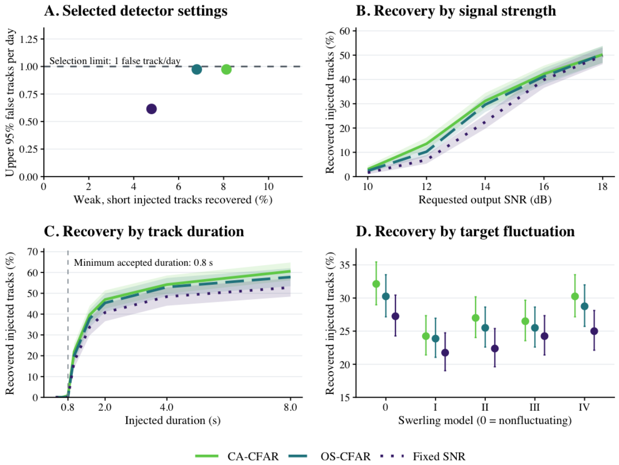
Figure 3.
Radar results from Tromsø and Svalbard. (A) Hourly Tromsø events. The matched group includes 46 matches under the main rules and three from the additional check. (B) Hourly Svalbard events, matched using only the main rules. (C) Svalbard match counts under different angular limits. The small vertical lines show the range of counts after six changes to the radar position. (D) Events found after rearranging short pieces of the radar data at each site, expressed as rates per day. Vertical lines extend to the 95% Poisson upper estimates. The dashed line marks the one event per day limit used at Tromsø.
Figure 3.
Radar results from Tromsø and Svalbard. (A) Hourly Tromsø events. The matched group includes 46 matches under the main rules and three from the additional check. (B) Hourly Svalbard events, matched using only the main rules. (C) Svalbard match counts under different angular limits. The small vertical lines show the range of counts after six changes to the radar position. (D) Events found after rearranging short pieces of the radar data at each site, expressed as rates per day. Vertical lines extend to the 95% Poisson upper estimates. The dashed line marks the one event per day limit used at Tromsø.
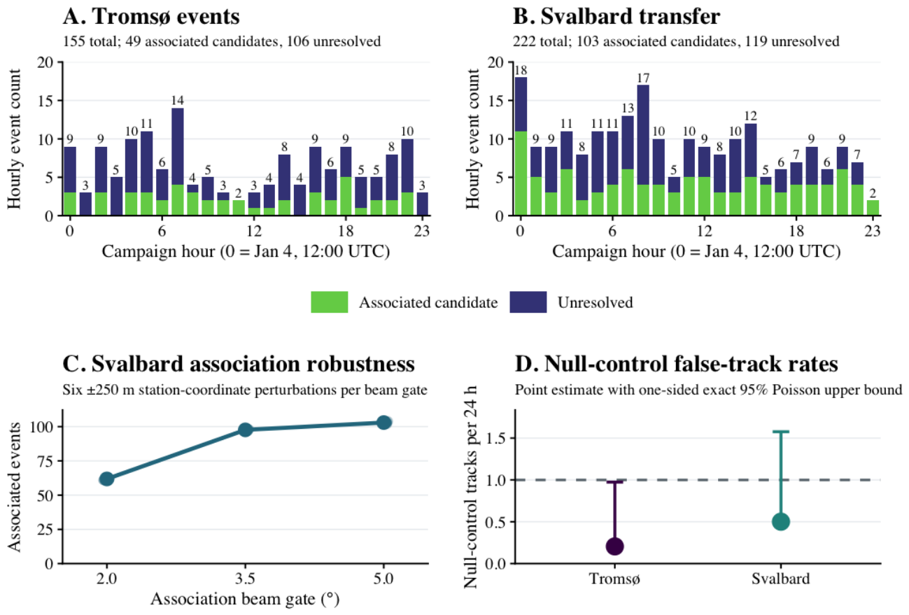
Figure 4.
Population learning in 300 simulated worlds, with 24 observations per schedule. (A) Remaining uncertainty relative to its value before observations. The same service weights were used to measure all five schedules. (B) Error in the estimated population compared with the true population in each world. Lines show averages from the approximate updates used during scheduling. Shaded areas show 95% bootstrap intervals for the mean at each observation. Table 1 compares the schedules after all 24 observations using the more thorough sampling method.
Figure 4.
Population learning in 300 simulated worlds, with 24 observations per schedule. (A) Remaining uncertainty relative to its value before observations. The same service weights were used to measure all five schedules. (B) Error in the estimated population compared with the true population in each world. Lines show averages from the approximate updates used during scheduling. Shaded areas show 95% bootstrap intervals for the mean at each observation. Table 1 compares the schedules after all 24 observations using the more thorough sampling method.
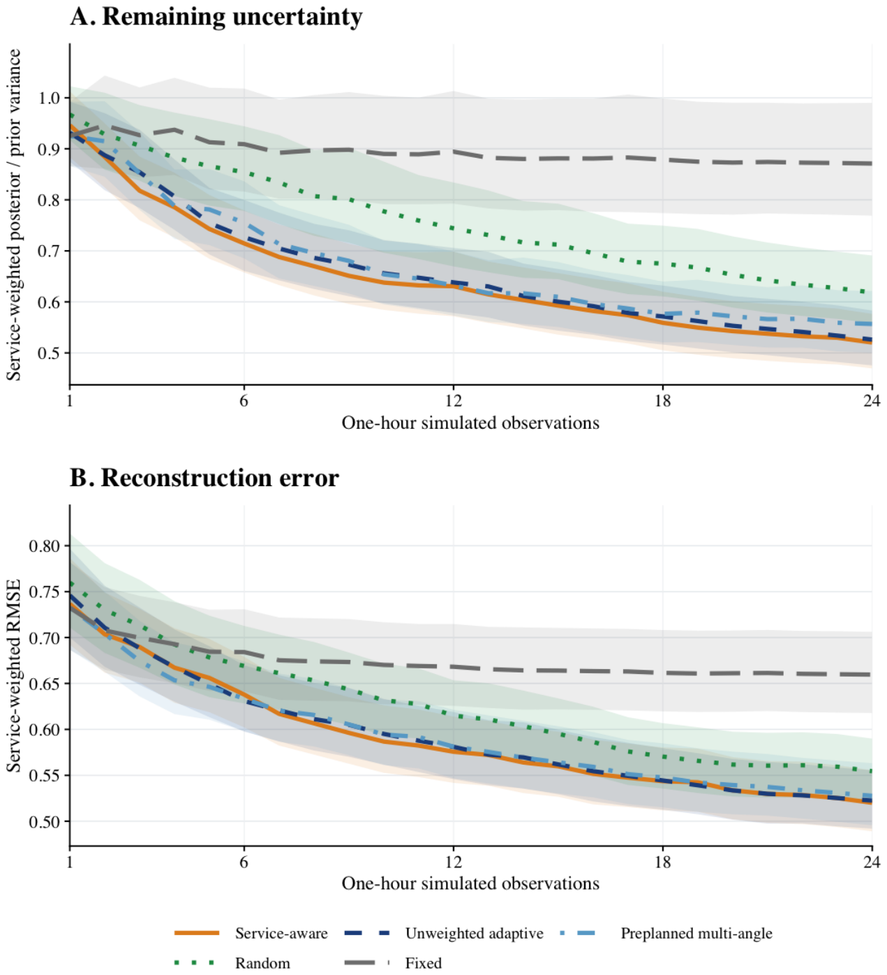
Figure 5.
Modeled radar response and pointing choices. (A) Share of the response coming from each altitude band at each elevation, using the ORDEM population of objects larger than 1 cm. The shares at each elevation add to one. (B) Elevations used across 300 simulated worlds. Larger dots indicate a greater fraction of observations at that elevation.
Figure 5.
Modeled radar response and pointing choices. (A) Share of the response coming from each altitude band at each elevation, using the ORDEM population of objects larger than 1 cm. The shares at each elevation add to one. (B) Elevations used across 300 simulated worlds. Larger dots indicate a greater fraction of observations at that elevation.
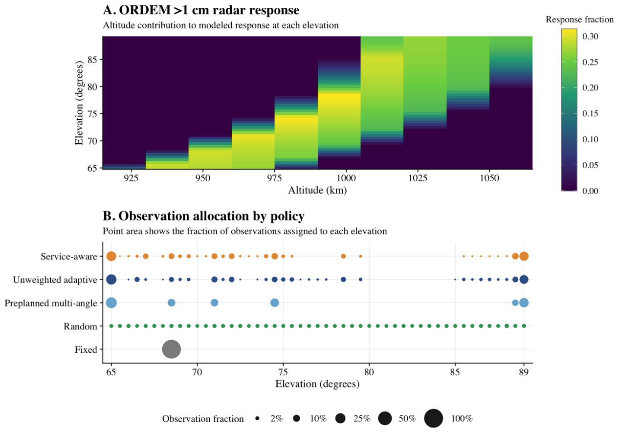

Table 1.
Results after 24 observations, using posterior samples from 300 paired simulated worlds. Each row compares adaptive scheduling with service weights against the named schedule. Positive percentages mean less uncertainty or lower error with service weights. Parentheses give 95% bootstrap intervals. The p values were adjusted across all eight comparisons using Holm’s method.
Table 1.
Results after 24 observations, using posterior samples from 300 paired simulated worlds. Each row compares adaptive scheduling with service weights against the named schedule. Positive percentages mean less uncertainty or lower error with service weights. Parentheses give 95% bootstrap intervals. The p values were adjusted across all eight comparisons using Holm’s method.
| Uncertainty reduction | RMSE reduction | |||
| Comparator | % (95% interval) | % (95% interval) | ||
| Fixed | 41.2 (37.8, 44.4) | 21.2 (18.0, 24.4) | ||
| Random | 15.4 (11.3, 19.4) | 6.04 (2.61, 9.41) | 0.00375 | |
| Preplanned (multiple angles) | 5.35 (3.03, 7.66) | 0.000314 | 1.16 (, 3.32) | 0.617 |
| Unweighted adaptive | 1.55 (, 3.53) | 0.400 | 0.29 (, 2.34) | 0.783 |
Disclaimer/Publisher’s Note: The statements, opinions and data contained in all publications are solely those of the individual author(s) and contributor(s) and not of MDPI and/or the editor(s). MDPI and/or the editor(s) disclaim responsibility for any injury to people or property resulting from any ideas, methods, instructions or products referred to in the content. |
© 2026 by the authors. Licensee MDPI, Basel, Switzerland. This article is an open access article distributed under the terms and conditions of the Creative Commons Attribution (CC BY) license (http://creativecommons.org/licenses/by/4.0/).
Copyright: This open access article is published under a Creative Commons CC BY 4.0 license, which permit the free download, distribution, and reuse, provided that the author and preprint are cited in any reuse.