A Simulative Investigation of The Effects and Sensitivity of Key Operating and Equipment Parameters on the Thermodynamic Performance of a Rankine Cycle

Roy Bou Hamdan

doi:10.20944/preprints202610.1003.v1

Submitted:

06 October 2026

Posted:

12 October 2026

You are already at the latest version

Abstract

Ranges of 5 values for 4 different process parameters in a rankine cycle (heater outlet temperature, turbine outlet pressure, pump outlet pressure, and turbine efficiency) were simulatively experimented with in DWSIM software (an open-source process simulation environment used to model and simulate chemical engineering processes under steady-state and dynamic conditions). These values were changed and three dependent variables were measured for each change: net power output, vapor molar fraction and thermal efficiency. Additionally, sensitivity coefficients to measure deviations for each variable were compared according to a set baseline. It was found that the changes in turbine efficiency directly correlated to most of the dependent variables in a linear relationship, while pump outlet pressure and turbine outlet pressure displayed quadratic relationships with the dependent variables. Heater outlet temperature displayed low sensitivity with thermal efficiency, and all such trends are noted in the article. The results provide insight into key operating parameters in Rankine cycles and how theoretical models display the changes in process efficiency. The results were simulated theoretically using a software, which does not necessarily provide output to realistic situations of Rankine cycles. The explicit values of theoretical calculations may not be present in realistic settings, however the general trends and sensitivity coefficients of each parameter and its dependent variable may help provide insight into changes in Rankine operating parameters.

Keywords:

rankine

;

rankine cycle

;

chemical engineering

;

thermodynamic modelling

;

thermodynamics

;

simulations

;

DWSIM

;

heater outlet temperature

;

turbine efficiency

;

thermal efficiency

;

turbine outlet pressure

;

net power output

;

vapor molar fraction

;

pump outlet pressure

;

materials chemistry

;

fluid mechanics

;

sustainable energy

;

green energy

;

green chemistry

Subject:

Chemistry and Materials Science - Chemical Engineering

I. Introduction

Global warming

A Rankine cycle is a thermodynamic cycle used for power generation. It converts heat from wasted fluid (such as water or organic fluids) back to electricity for reuse (Kasaeian et al., 2022, p. 1). Specifically, they are also used in small modular reactors (SMRs) which are alternative nuclear reactors (to the traditional nuclear plant) that are more flexible in terms of location, while being affordable (Kim et al., 2025, p. 1). SMRs rely heavily on Rankine cycles to regenerate wasted water to electricity.

A simple Rankine cycle consists of a boiler, expander, condenser and pumping unit (Tarrad, 2022, p. 4). When a Rankine cycle is used to recover heat into mechanical energy, first the fluid is pumped to high pressures, then it is heated until the boiling point (at least) in order for the entirety of the fluid to be in vapor form (“Rankine cycle,” 2024). Preheating the fluid is significant to the process since the expansion that occurs in the turbine creates a substantial drop in temperature. When the high-pressure gas enters the expander (turbine) the stream hits the stationary nozzles with high stored thermal energy (enthalpy) which creates kinetic energy that is later converted to rotational mechanical energy when it hits the curved rotating motor blades. This mechanical energy results in power generation at the turbine shaft, and this energy can be directed to an electrical generator to be converted to usable electricity (Smith et al., 2021, p. 249) (Turboden, 2026).

Although there is extensive research available on Rankine cycle performance, further analysis of the impacts of individual operating and equipment parameters and conditions remain valuable to understanding effective decisions in an SMR that need to be made or altered. This study investigates the effects of heater outlet temperature, pump outlet pressure, turbine outlet pressure, and turbine efficiency, using a DWSIM model of the Rankine cycle. The performance of the cycle will be evaluated and analyzed using net power output, thermal efficiency, and outlet vapor fraction. Sensitivity coefficients and relative change analyses will be used in order to quantify the influence of each investigated parameter on the thermodynamic performance of the simulated Rankine cycle model. This approach will provide a quantitative assessment of parameter influence aside from the trends observed from the results of the simulation.

II. Methodology

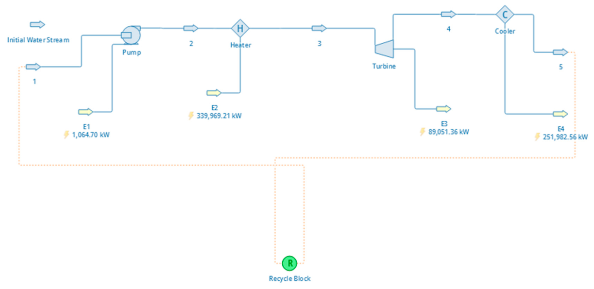
For the application of this investigation, a steady-state model of the Rankine cycle was created in DWSIM. The model included a pump, heater (boiler), expander (turbine), and cooler. The cooler was connected to a recycle logic block to reattach the stream to the pump to create a closed loop. To kickstart the cycle, a material stream of water was created and connected to the pump. After the cycle began, the material stream was removed and the recycle block outlet was connected to the pump.

Figure 1. The simulated Rankine Cycle (DWSIM).

II.I. Baseline Parameters

For the initial stream of water, the mass flow was chosen to be 114 kg/s (6327.96 mol/s) based on a paper by Yin et al., 2026. The mass flow was kept constant for all variables that were manipulated, and so was the initial temperature and pressure (313.15 K and 101325 Pa). “Baseline” parameters were established to compare the findings to. For heater outlet temperature, 673.15 K (or 400° C) was chosen, the pump outlet pressure was chosen as 7,000,000 Pa (7 MPa), the turbine outlet pressure as 50,000 Pa, and the pump and turbine efficiencies as 75% (default on DWSIM). These values were used for every trial except if the variable was being manipulated. Additionally, the cooler outlet temperature was set to 313.15 K (same as the initial stream). The baseline values were chosen because they produced a vapor molar fraction of about 0.924 (92.4%) which was not too wet and enough to work as a middle comparable value. Additionally, no value above 823.15 K was used for heater outlet temperature since the vapor molar fraction became 1 at that point.

Range of heater outlet temperature:

623.15, 673.15, 723.15, 773.15, and 823.15 in Kelvin (with 673.15 being the baseline)

Or 350, 400, 450, 500, and 550 in degrees Celsius.

Range of turbine outlet pressure:

10,000, 25,000, 50,000, 75,000, and 100000 in Pascals (with 50,000 being the baseline)

Range of pump outlet pressure:

3,000,000, 5,000,000, 7,000,000, 9,000,000, and 11,000,000 in Pascals (with 7,000,000 being the baseline)

Or 3, 5, 7, 9, and 11 MPa

Range of turbine efficiency:

65, 70, 75, 80, and 85 in % (with 75 being the baseline)

II.II. Equations Used

The performance of the Rankine cycle was evaluated using the following thermodynamic relationships:

W_net = W_turbine − W_pump

(1)

η_{thermal} = \frac{W_{net}}{Q_{in}}

(2)

% Δ Y = \frac{{Y_{i} - Y}_{baseline}}{Y_{baseline}} \times 100

(3)

S = \frac{\frac{Δ Y}{Y}}{\frac{Δ X}{X}}

(4)

Where:

W represents the power output/consumption
η represents efficiency
Q represents heat input
%ΔY represents percent change in the variable relative to the baseline value
Y_i represents the value attained after parameter manipulation (dependent variable)
Y_baseline represents the baseline value of the parameter measured
S represents the sensitivity coefficient
X represents the investigated parameter (independent)
Y represents the result of the investigated parameter (dependent)

II.III Additional Calculations

The net power was used to evaluate electrical output, while the thermal efficiency was for comparing conversion effectiveness. The vapor fraction evaluated the exhaust quality of the turbine, and the sensitivity coefficients compared each parameter in terms of significance. Regression analysis was mainly performed using linear and second order polynomial trend models. The coefficient of determination (R²) was also calculated so that the correlation between investigated parameters could be evaluated. All calculations relating to the graphing were done with Microsoft Excel.

III. Raw Data

Table 1. Effect of Heater Outlet Temperature on Rankine Cycle Performance.

Heater Outlet Temperature (K)	623.15	673.15	723.15	773.15	823.15
Pump Power Consumption (kW)	1064.7	1064.7	1064.7	1064.7	1064.7
Turbine Power Output (kW)	323752	339969	354683	368714	382426
Heater Duty (kW)	73072.8	78574.7	84002.4	89537.2	95252.1
Cooler Duty (kW)	251744	262459	271745	280241	288239
Turbine Outlet Vapor Fraction	0.883131	0.923913	0.959255	0.991593	1.000000
Net Power (kW)	72008.1	77510	82937.7	88472.5	94187.4
Thermal Efficiency	0.222417	0.227991	0.233836	0.239949	0.246289

Table 2. Effect of Turbine Outlet Pressure on Rankine Cycle Performance.

Turbine Outlet Pressure (Pa)	10000	25000	50000	75000	100000
Pump Power Consumption (kW)	1070.85	1068.54	1064.7	1060.86	1057.02
Turbine Power Output (kW)	339967	339968	339969	339971	339972
Heater Duty (kW)	95508.8	86207.8	78574.7	73843	70356.7
Cooler Duty (kW)	245529	254829	262459	267188
Turbine Outlet Vapor Fraction	0.89023	0.908527	0.923913	0.933703	0.941082
Net Power (kW)	94437.95	85139.26	77510	72782.14	69299.68
Thermal Efficiency	0.277786	0.250433	0.227991	0.214083	0.203839

Table 3. Effect of Pump Outlet Pressure on Rankine Cycle Performance.

Pump Outlet Pressure (Pa)(x 10⁶)	3	5	7	9	11
Pump Power Consumption (kW)	451.924	758.313	1064.7	1371.09	1677.48
Turbine Power Output (kW)	348843	344549	339969	335063	329782
Heater Duty (kW)	70430.3	75778	78574.7	80052.6	80676.3
Cooler Duty (kW)	278865	269529	262459	256381
Turbine Outlet Vapor Fraction	0.986353	0.950823	0.923913	0.90078	0.879472
Net Power (kW)	69978.38	75019.69	77510	78681.51	78998.82
Thermal Efficiency	0.200601	0.217733	0.227991	0.234826	0.239549

Table 4. Effect of Turbine Efficiency on Rankine Cycle Performance.

Turbine Efficiency (%)	65	70	75	80	85
Pump Power Consumption (kW)	1064.7	1064.7	1064.7	1064.7	1064.7
Turbine Power Output (kW)	339969	339969	339969	339969	339969
Heater Duty (kW)	68098.1	73336.4	78574.7	83813	89051.4
Cooler Duty (kW)	272936	267698	262459	257221	251983
Turbine Outlet Vapor Fraction	0.963787	0.94385	0.923913	0.903976	0.884038
Net Power (kW)	67033.4	72271.7	77510	82748.3	87986.7
Thermal Efficiency	0.197175	0.212583	0.227991	0.2434	0.258808

The raw data was graphically visualized by comparing each variable to the net power, vapor outlet fraction, and thermal efficiency. As stated in the methodology, regression analysis was done on excel by creating a trendline and calculating its equation.

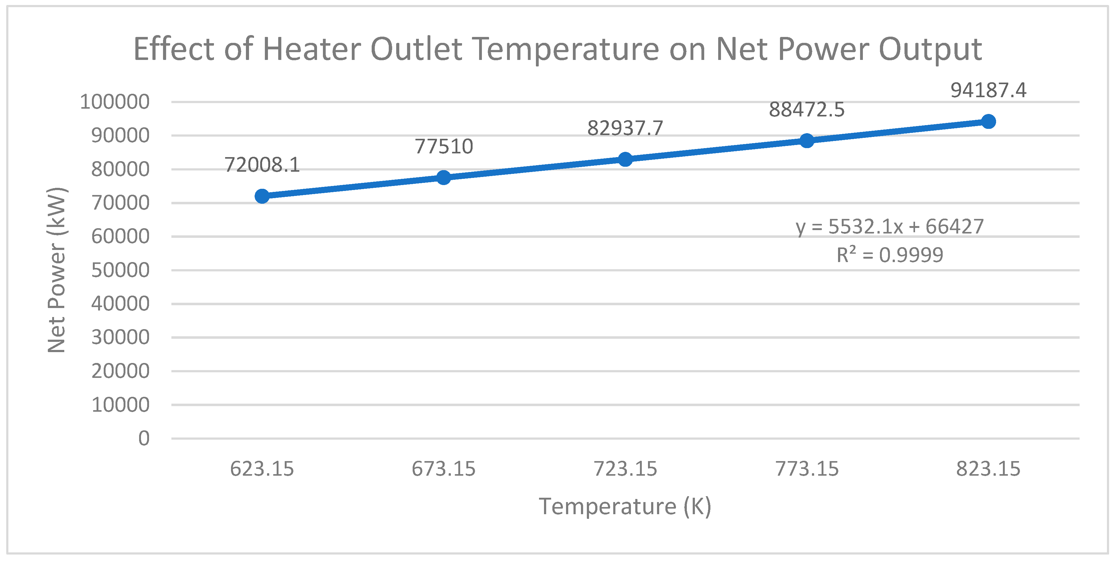
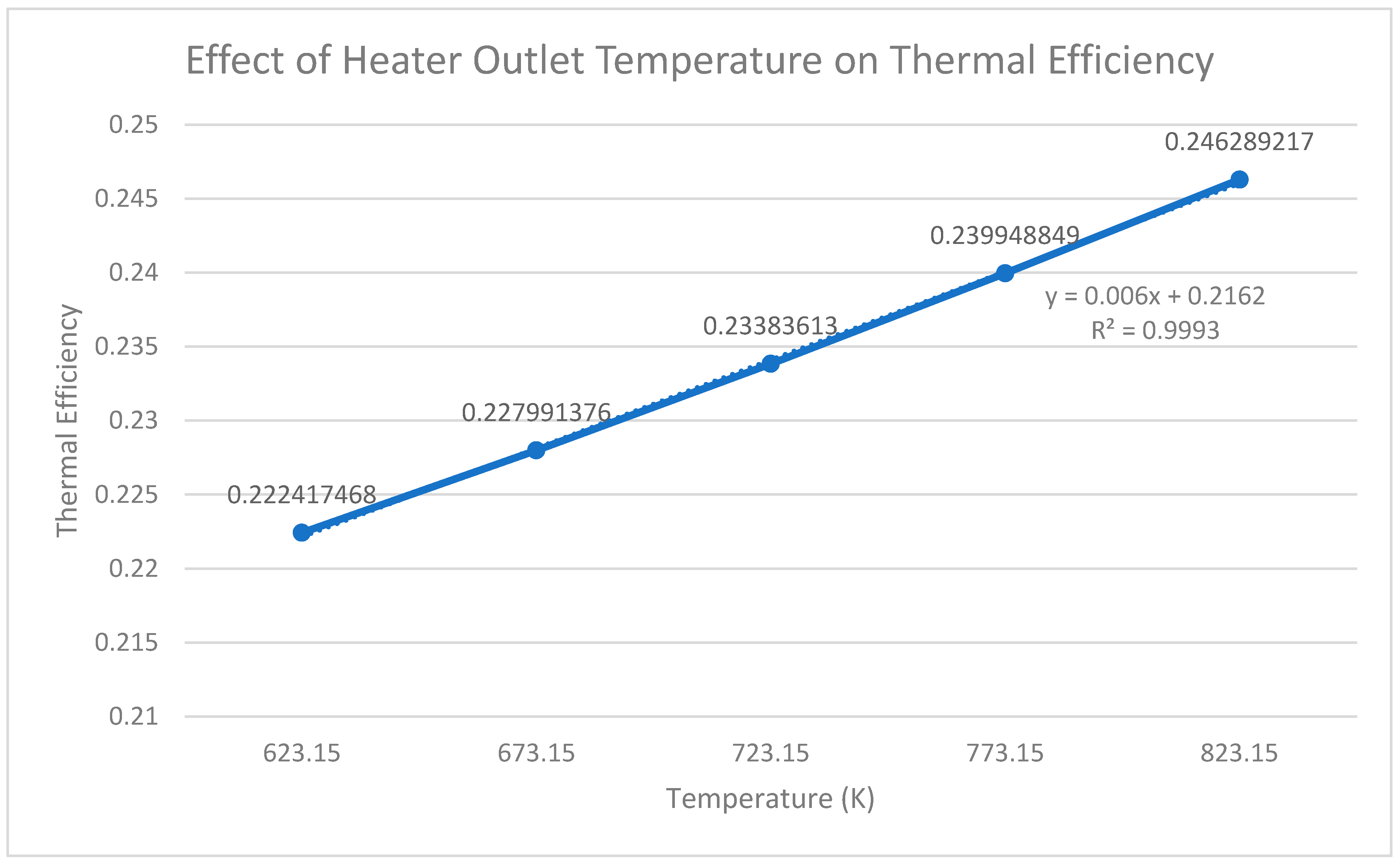
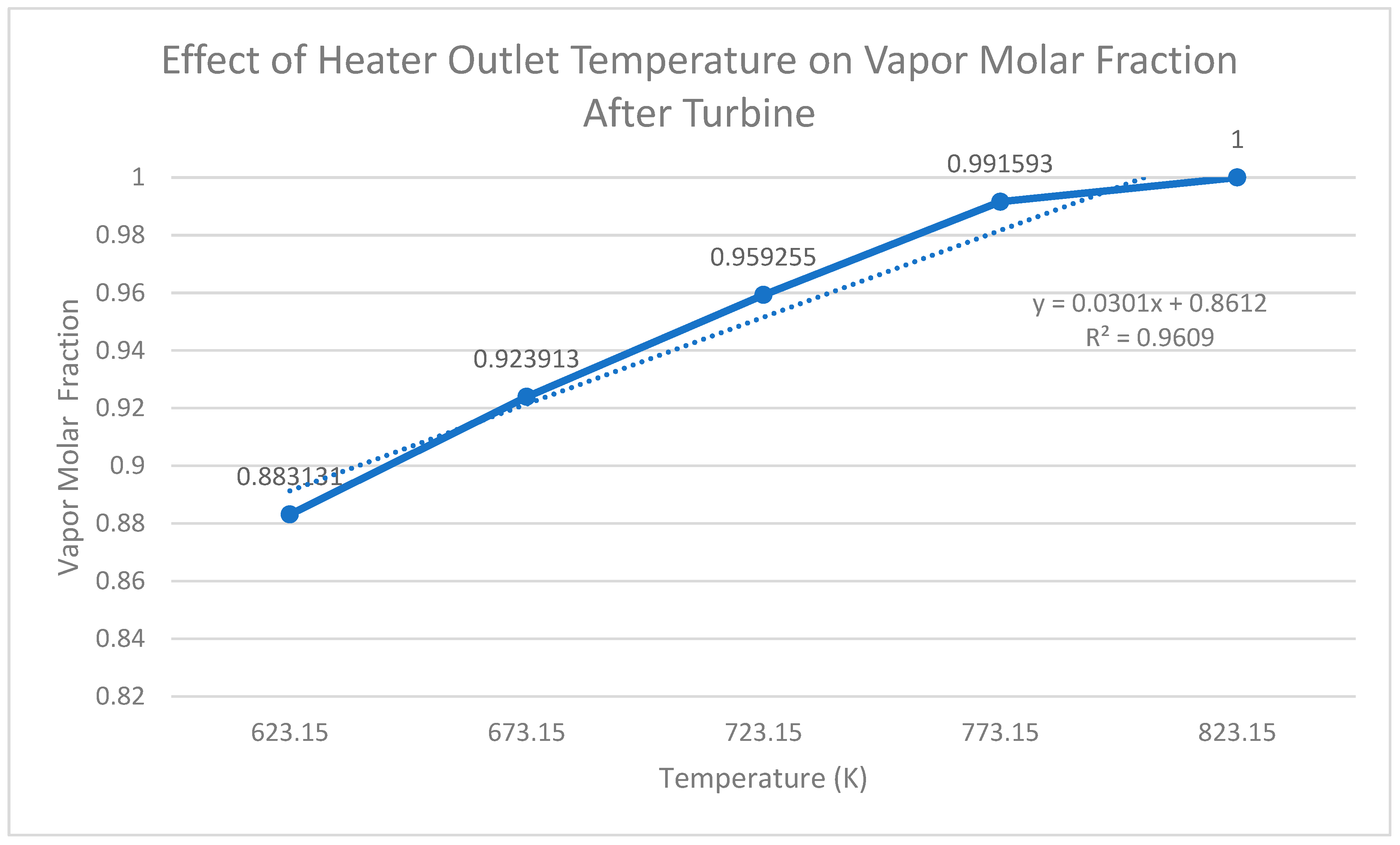
For the graphs relating heater outlet temperature to net power, vapor outlet fraction, and thermal efficiency, a linear trend line was chosen because the relationship between them exhibited an approximately proportional increase over the evaluated range. Additionally, the linear model provided a coefficient of determination (R²) value close to 1 for each dependent variable. The only exception is Graph 3, where the model mathematically predicted an increase to a value greater than 1, which is not possible in the case of vapor molar fraction.

Graph 1. Effect of Heater Outlet Temperature on Net Power Output.

Graph 2. Effect of Heater Outlet Temperature on Thermal Efficiency.

Graph 3. Effect of Heater Outlet Temperature on Vapor Molar Fraction After Turbine.

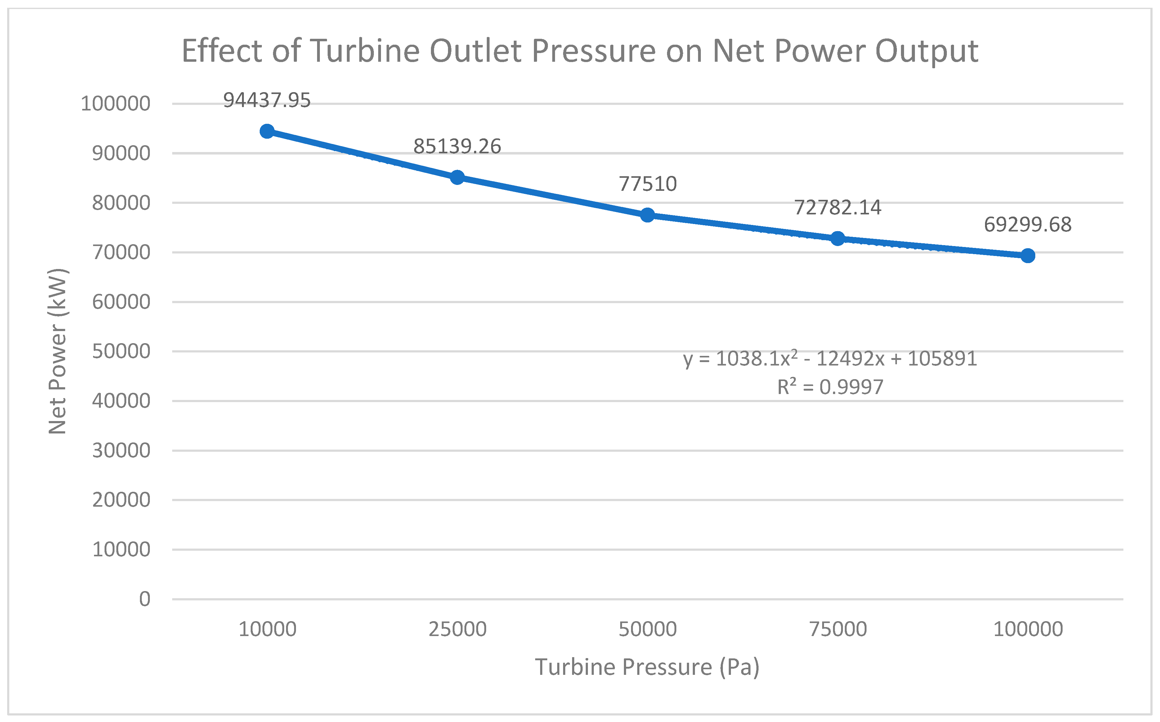
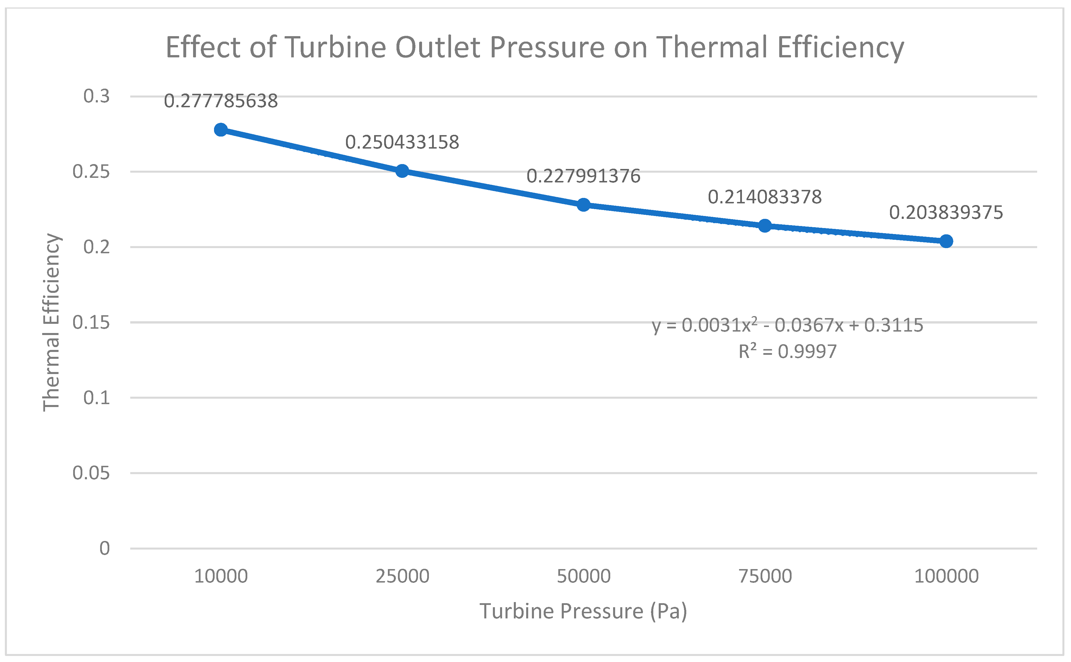
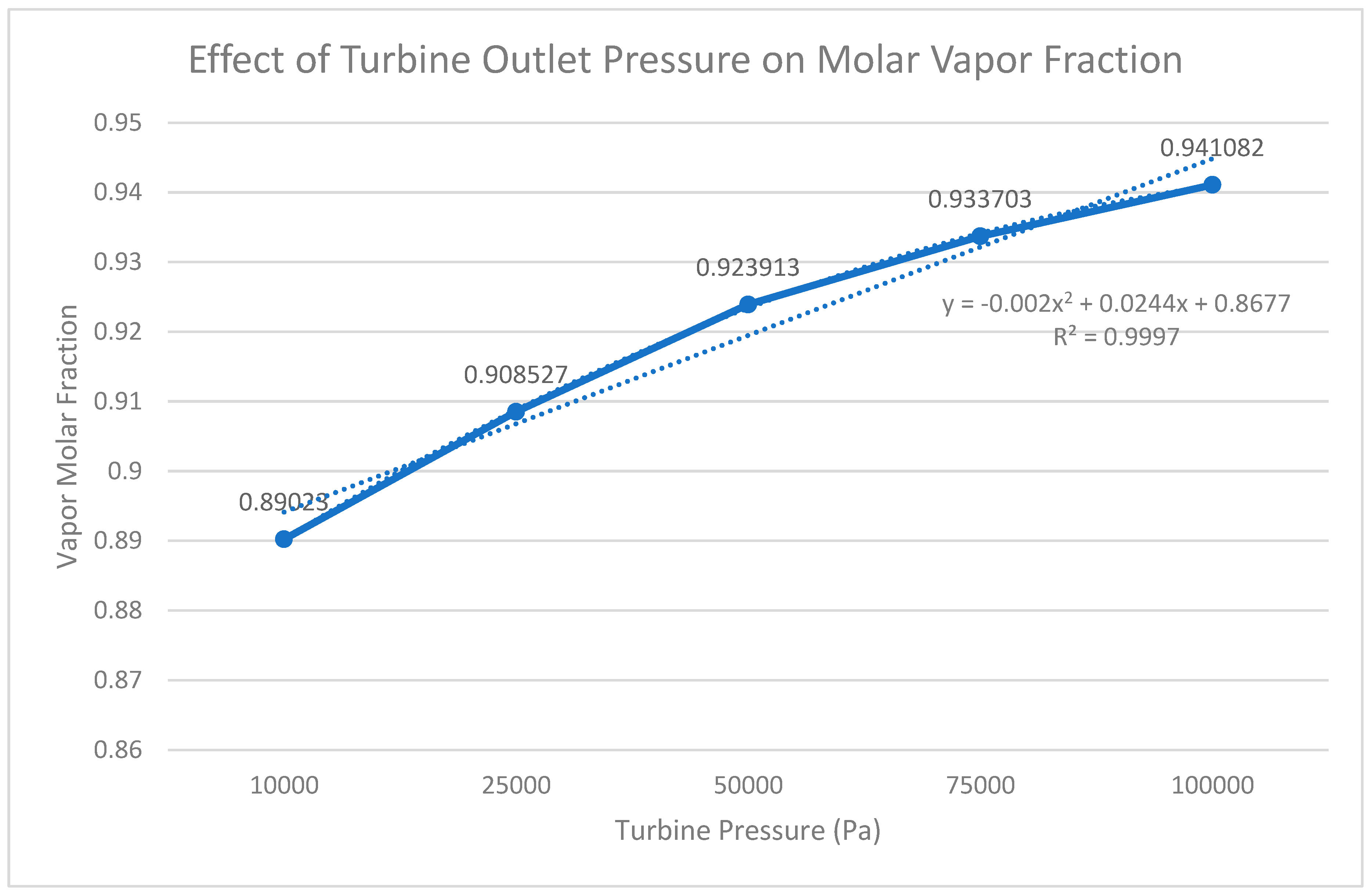
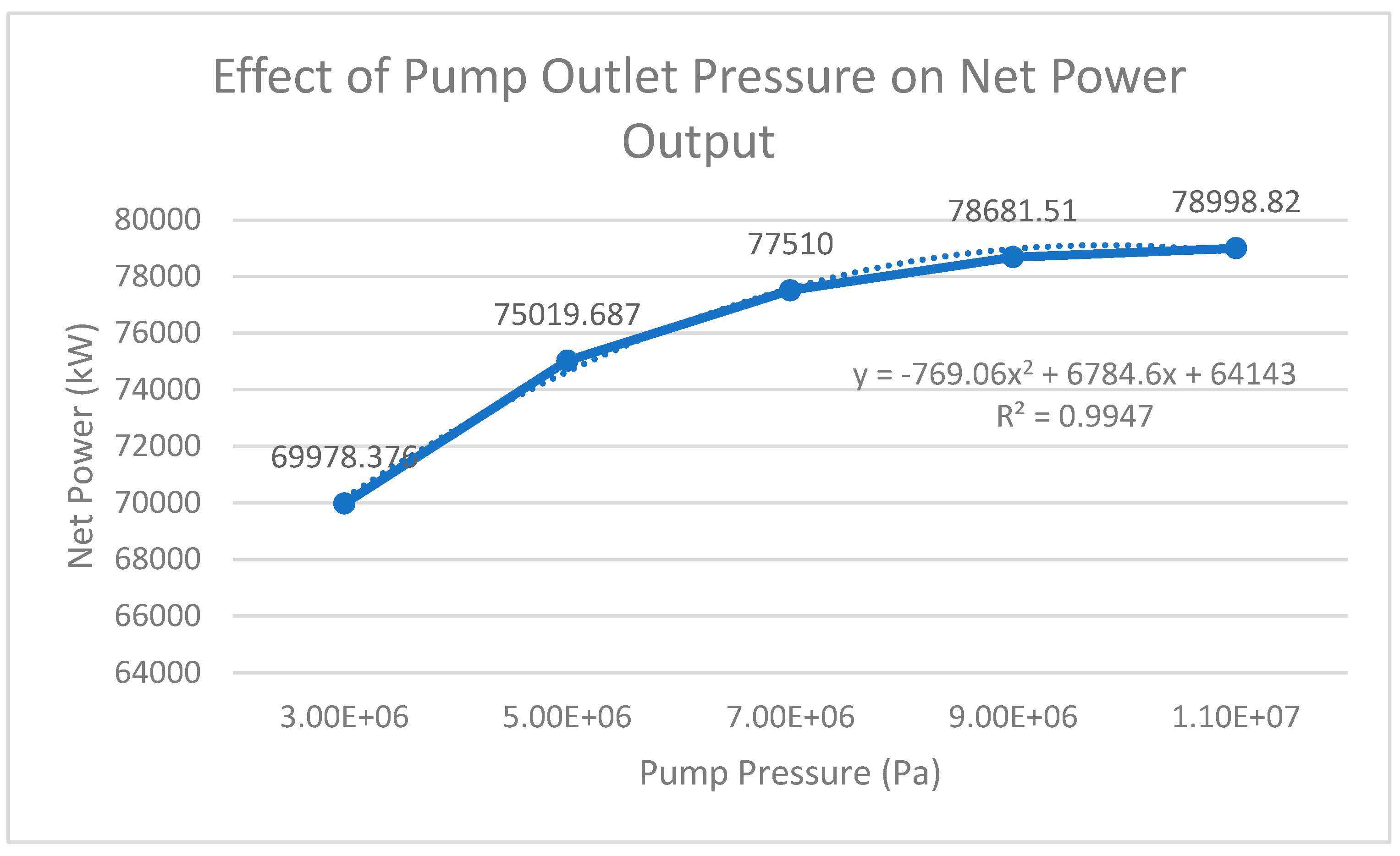
For the next two of the relationships between the independent (turbine outlet pressure and pump outlet pressure) and dependent variables, a difference in regression analysis should be noted. A second-order polynomial trendline (instead of a linear one) was selected mainly due to the fact that their relationships exhibited nonlinear behaviors over each operating range. As a result, the second-order polynomial model provided the best fit to the data collected, as supported by higher coefficients of determination (R²).

Graph 4. Effect of Turbine Outlet Pressure on Net Power Output.

Graph 5. Effect of Turbine Output Pressure on Thermal Efficiency.

Graph 6. Effect of Turbine Outlet Pressure on Molar Vapor Fraction.

Graph 7. Effect of Pump Outlet Pressure on Net Power Output.

Graph 8. Effect of Pump Outlet Pressure on Thermal Efficiency.

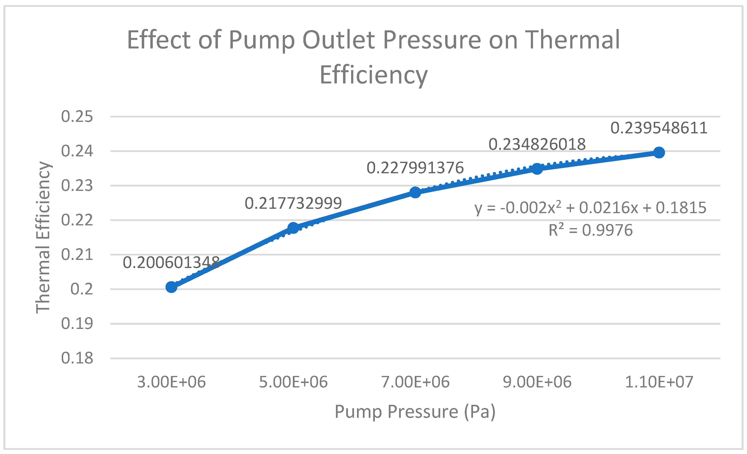
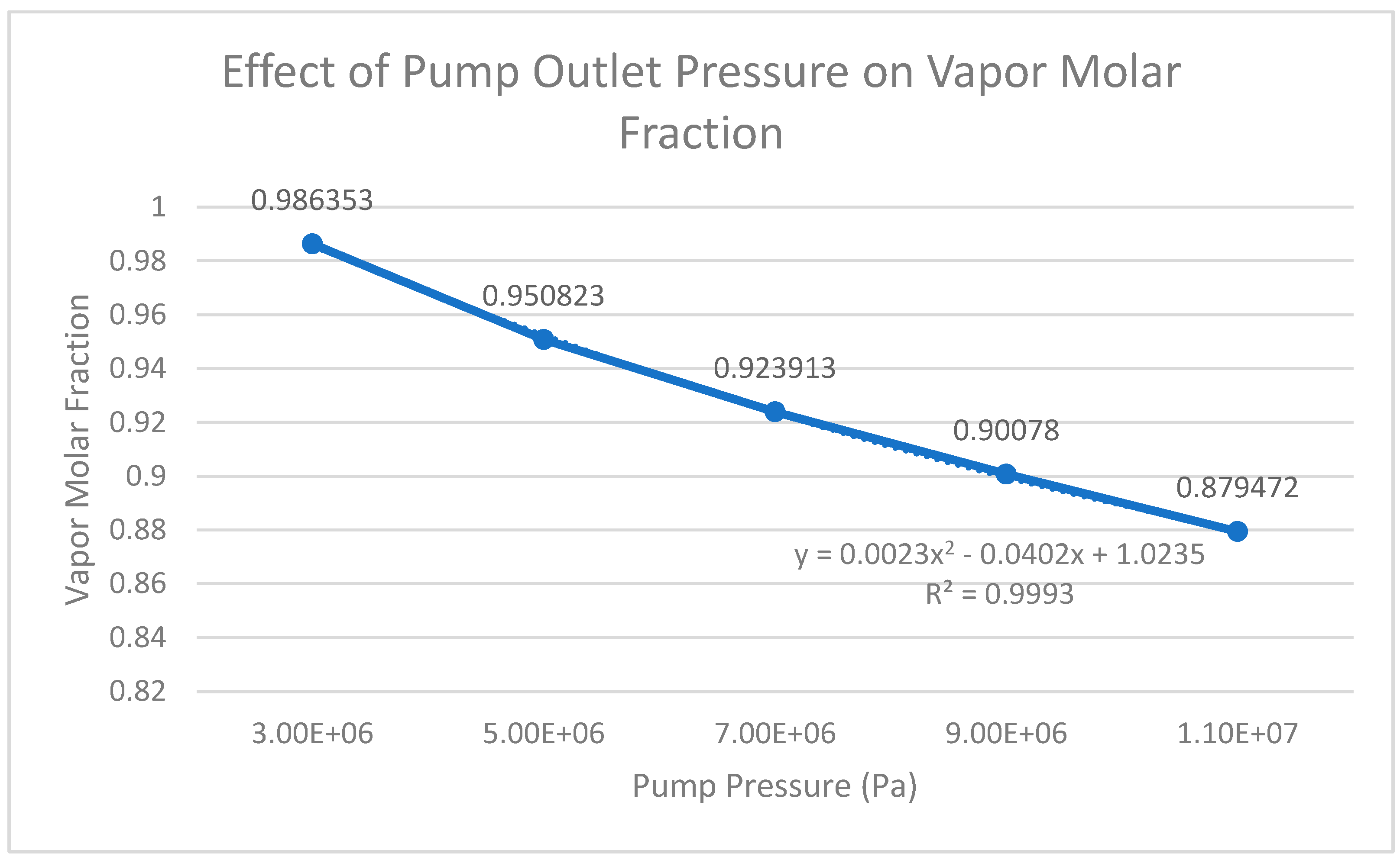
Graph 9. Effect of Pump Outlet Pressure on Vapor Molar Fraction.

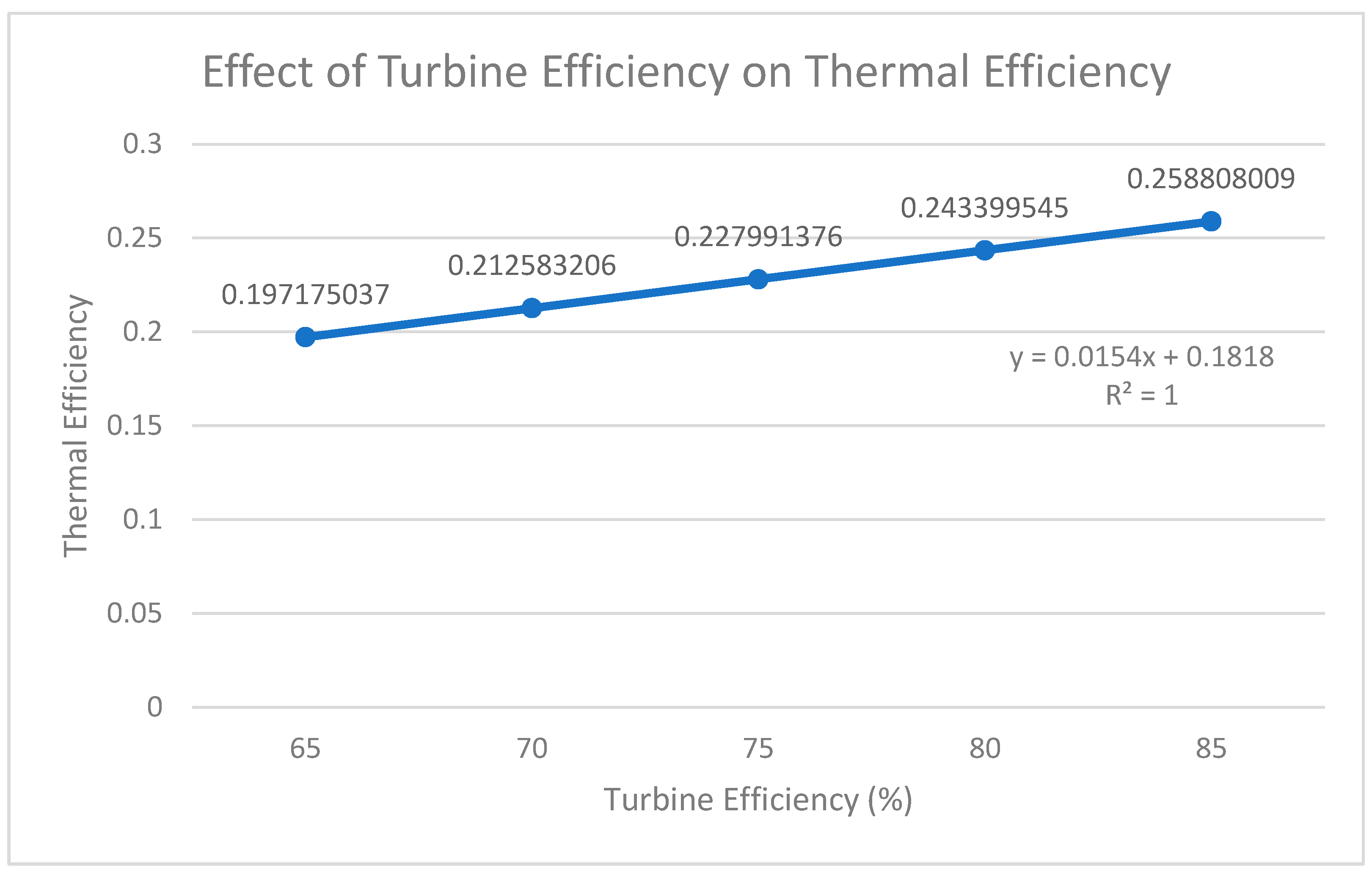
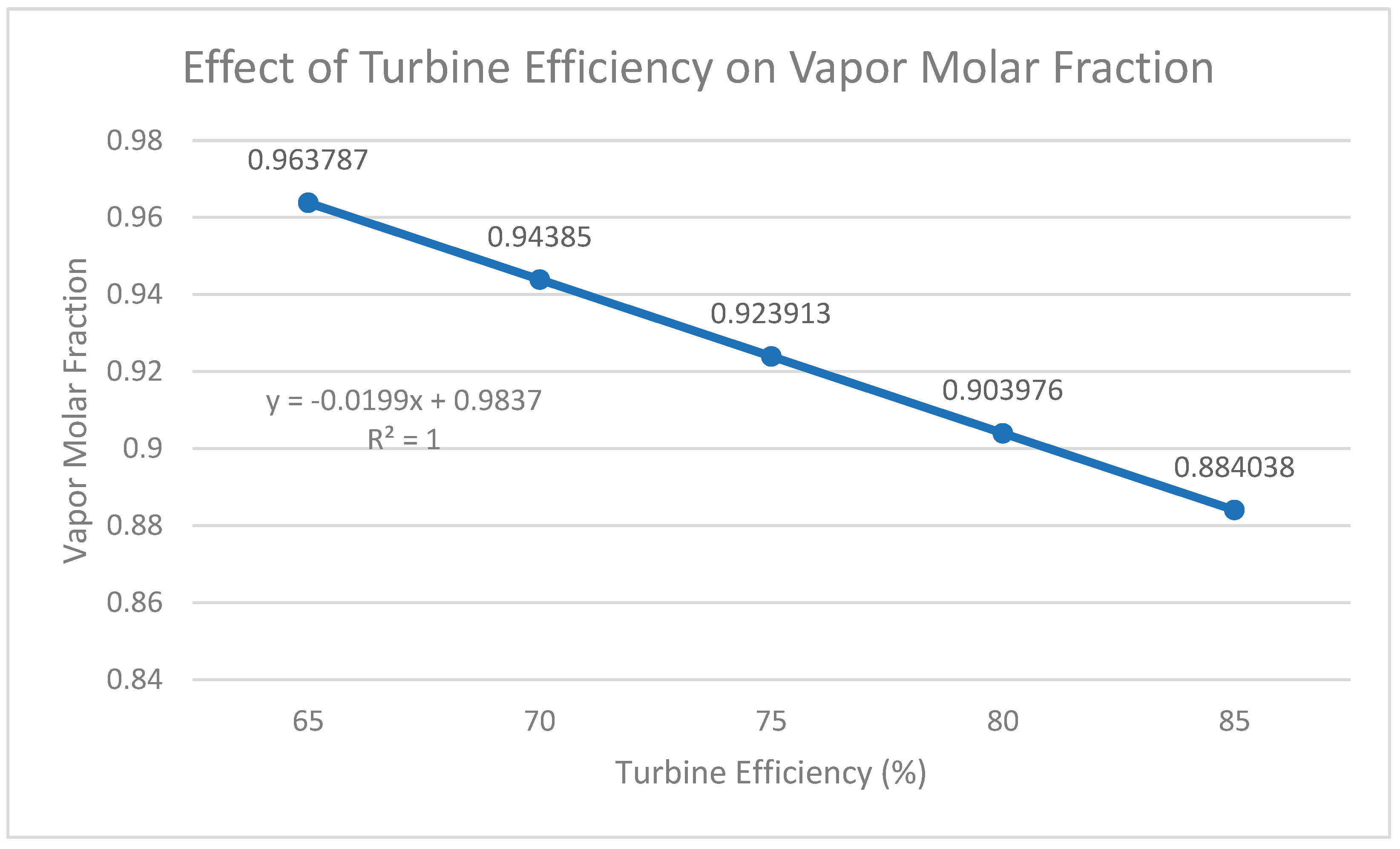
For the turbine efficiency, it was visually represented as linear. This variable was less of a surprise, and it is widely accepted that turbine efficiency is directly related to (and proportional to) net power output (and therefore thermal efficiency and vapor molar fraction) (Alshammari et al., 2024, p. 10). Hence, the coefficient of determination (R²) of each graph is exactly 1.

Graph 10. Effect of Turbine Efficiency on Net Power Output.

Graph 11. Effect of Turbine Efficiency on Thermal Efficiency.

Graph 12. Effect of Turbine Efficiency on Vapor Molar Fraction.

IV. Discussion

IV.I Heater Outlet Temperature

To reflect on the first variable that was manipulated, the heater outlet temperature, the graph represents a clear trend for each variable (graphs 1, 2, and 3). For graph 1, when the outlet heater temperature decreased to 623.15 K (350° C) the net power decreased significantly as well, and vice versa. The percentage change of each temperature variable relative to the baseline can be calculated using equation 3, and this represents how much the outlet temperature increases or decreases relative to the baseline.

For 623.15 K, the net power percentage decrease relative to the baseline was 7.10%.

While for higher temperatures, their percentage increase from the baseline were as follows:

Table 5. Effect of Outlet Temperature on Net Power Output Deviation from the Baseline.

Heater Outlet Temperature (K)	Net Power Output Deviation
723.15	7.00% increase
773.15	14.14% increase
823.15	21.52% increase

The net power output increased progressively relative to the baseline as heater outlet temperature increased.

By calculating the sensitivity coefficient of each temperature (equation 4), we can quantify the relative response of net power output (and the other variables) to changes in heater outlet temperature (and the rest of the parameters investigated).

For 623 K, the calculated sensitivity coefficient was 0.96, which means that as the heater outlet temperature decreases by 1% relatively, it corresponds to a 0.96% relative decrease in the net power output. For the rest of the temperatures, the sensitivity coefficient was:

Table 6. Effect of Outlet Temperature on Net Power Output Sensitivity.

Heater Outlet Temperature (K)	Sensitivity Coefficient
723.15	0.94
773.15	0.95
823.15	0.97

For all of the temperatures the sensitivity coefficients are quite high, indicating that the net power output is very sensitive to changes in the heater outlet temperature. Since w_t = h_in − h_out for a steady-flow turbine, as heater outlet temperature increases, the inlet temperature increases, meaning the inlet enthalpy will increase, causing the drop in enthalpy to be greater and in need of greater work from the turbine (Moran, et al., 2011). Additionally, the values fluctuate around a similar number, showing that sensitivity is mostly constant across all investigated parameters. This is consistent with the data that is collected, and the information that is revealed about the net output power’s sensitivity to heater outlet temperature.

In terms of thermal efficiency (graph 2), the percentage change of each temperature relative to the baseline was calculated using the same equation (equation 3):

Table 7. Effect of Outlet Temperature on Thermal Efficiency Deviation from the Baseline.

Heater Outlet Temperature (K)	Thermal Efficiency Deviation
623.15	2.44% decrease
723.15	2.56% increase
773.15	5.24% increase
823.15	8.03% increase

And the sensitivity coefficients were calculated with equation 4:

Table 8. Effect of Outlet Temperature on Thermal Efficiency Sensitivity.

Heater Outlet Temperature (K)	Sensitivity Coefficient
623.15	0.27
723.15	0.28
773.15	0.35
823.15	0.36

When analyzing the sensitivity coefficient at each temperature, it seems that they are less constant than other variables. This suggests that thermal efficiency is more sensitive to changes in outlet temperature at higher temperatures. Additionally, for each 1% change in temperature, thermal efficiency changes from 0.27%-0.36%, which is considerably low, suggesting that thermal efficiency is proportional to the heater outlet temperature (when considering graph 2), however it is not as sensitive to it as much as net power output.

Finally, for the effect of heater outlet temperature on vapor molar fraction, graph 3 reveals that the vapor molar fraction is also generally positively proportional to the heater outlet temperature, however the R² value appears to be lower for this graph (0.9609 in comparison to the previous two variables, which had coefficients of determinations greater than 0.99). This is explained by the fact that the mathematical calculation that Excel created for the trendline predicts the vapor fractions at higher temperatures to be greater than 1, which is physically impossible. This can be regarded as a limitation of this graph.

Table 9. Effect of Outlet Temperature on Vapor Molar Fraction Deviation from the Baseline.

Heater Outlet Temperature (K)	Vapor Molar Fraction Deviation
623.15	4.41% decrease
723.15	3.83% increase
773.15	7.33% increase
823.15	8.23% increase

Table 10. Effect of Outlet Temperature on Vapor Molar Fraction Sensitivity.

Heater Outlet Temperature	Sensitivity Coefficient
623.15	0.59
723.15	0.51
773.15	0.49
823.15	0.36

The vapor molar fraction deviates less as temperature increases, which can be justified since it is increasingly closer to 1. However, in terms of the sensitivity, it decreases as temperature rises, suggesting that at higher temperatures the vapor molar fraction is less sensitive to changes in temperatures. This behavior is consistent with the explanation suggested previously. The vapor molar fraction is reaching its physical upper limit, and as the outlet reaches an almost fully vaporized state, further increases in temperature start to produce progressively smaller changes in the vapor fraction.

Additionally, it is worth noting that vapor molar fraction is more susceptible to changes in temperature than thermal efficiency, since the lowest sensitivity coefficient of VMF is equal to the highest in thermal efficiency, and the rest of the values are considerably higher. Nonetheless, net power output is the most susceptible variable to temperature changes, as displayed by its relatively high sensitivity coefficients that outperform VMF and thermal efficiency by a large measure. Consequently, because the net power output displayed the highest sensitivity, its deviation at higher temperatures (compared to the baseline) was more than double the percentage deviations of thermal efficiency and vapor molar fraction

IV.II. Turbine Outlet Pressure

Regarding the graphs of the effects of turbine outlet pressure, a second-degree polynomial trendline was calculated using excel. The simulated results exhibited nonlinear behavior, which can be explained by the drop in enthalpy that occurs as outlet pressure increases. Additionally, the coefficient of determination (R²) value for graphs 4, 5, and 6 respectively are 0.9997, 0.9997, and 0.9997. They are all extremely close to 1, therefore they display clear quadratic relationships mathematically.

As the turbine pressure increased, the net power output decreased, and vice versa (graph 4). For thermal efficiency, the conclusion was similar, with the highest turbine pressure was equated to the lowest thermal efficiency, etc. In terms of the vapor molar fraction, the percentage of the product that was vaporized increased as the pressure increased and decreased as the pressure decreased from the baseline.

Table 11. Effect of Turbine Outlet Pressure on Net Power Output Deviation from the Baseline.

Turbine Outlet Pressure (Pa)	Net Power Output Deviation
10,000	21.84% increase
25,000	9.84% increase
75,000	6.10% decrease
100,000	10.59% decrease

Table 12. Effect of Turbine Outlet Pressure on Net Power Output Sensitivity.

Turbine Outlet Pressure (Pa)	Sensitivity Coefficient
10,000	0.27
25,000	0.19
75,000	0.12
100,000	0.11

In Table 11 it can be seen that at lower pressures the deviations of the net power outputs were higher at lower outlet pressures (compared to the baseline). This is complemented by Table 12, which reveals that the sensitivity of net power output on the change in turbine outlet pressure dramatically decreases as pressure increases. At the lowest pressure, the sensitivity coefficient is about 145% more than the sensitivity coefficient at the highest pressure. This is a stark contrast to the effect of heater temperature on net power output. The sensitivity coefficients are considered quite low, especially at higher pressures, and even though they are mathematically related, it reveals the net power output is not as affected by the outlet pressure as it is by other variables.

Table 13. Effect of Turbine Outlet Pressure on Thermal Efficiency Deviation from the Baseline.

Turbine Outlet Pressure (Pa)	Thermal Efficiency Deviation
10,000	21.84% increase
25,000	9.84% increase
75,000	6.10% decrease
100,000	10.59% decrease

Table 14. Effect of Turbine Outlet Pressure on Thermal Efficiency Sensitivity.

Turbine Outlet Pressure (Pa)	Sensitivity Coefficient
10,000	0.27
25,000	0.19
75,000	0.12
100,000	0.11

Immediately, it can be noticed that the deviations and sensitivity of thermal efficiency are the same as the ones of the net power output. This can be explained by looking back at Table 2, which verifies that the heater duty was approximately constant throughout the entire variation of turbine outlet pressure. In fact, the heater duty only increased by about 0.0015%. Since the equation of thermal efficiency is dependent on the net power divided by the heat input (equation 2), and the heat input stayed essentially the same for every pressure input, the deviation and sensitivities of the thermal efficiency values should mimic those of the net power output.

Hence, what was said about the relationship between the net power output and the turbine outlet pressure can be reiterated for the values attributed to thermal efficiency. The sensitivity coefficients are quite low, representing a low dependency on this variable, and the sensitivity decreases as the pressure increases, as is displayed in tables 13 and 14.

Table 15. Effect of Turbine Outlet Pressure on Vapor Molar Fraction Deviation from the Baseline.

Turbine Outlet Pressure (Pa)	Vapor Molar Fraction Deviation
10,000	3.65% decrease
25,000	1.67% decrease
75,000	1.06% increase
100,000	1.86% increase

Table 16. Effect of Turbine Outlet Pressure on Vapor Molar Fraction Sensitivity.

Turbine Outlet Pressure (Pa)	Sensitivity Coefficient
10,000	0.05
25,000	0.03
75,000	0.02
100,000	0.02

As the outlet pressure increases, the turbine expansion becomes less extensive thereby prompting a higher vapor molar fraction in the product after the turbine. The relatively small changes in vapor molar fraction relative to the baseline (Table 15), along with the miniscule sensitivity coefficients (Table 16), can be attributed to the fact that the vapor molar fraction is close to throughout the entire investigation. However, it is worth noting especially that the vapor molar fraction is especially insensitive to the turbine outlet pressure. Even though graph 6 represents a strong positive correlation between the turbine outlet pressure and the VMF, the scale of the sensitivity of the VMF to the turbine outlet pressure is comparatively low. Additionally, the declining coefficient further indicates that its sensitivity decreases over the investigated range as it approaches a molar coefficient of 1 (Table 16).

IV.III. Pump Outlet Pressure

For the dependent variables measured as a result of pump outlet pressure, a second-degree polynomial trendline was also applied to the three dependent variables. The effects of pump outlet pressure on net power output and thermal efficiency both displayed positive proportional correlations, with an R² value of 0.9947 and 0.9976 respectively. By contrast, the effect of pump outlet pressure on VMF was proportionally decreasing, with an R² coefficient of 0.9993. All three variables observed represented a strong correlation in response to changes in pump outlet pressures, especially when they were modeled with a second-degree polynomial trendline.

Table 17. Effect of Pump Outlet Pressure on Net Power Output Deviation from the Baseline.

Pump Outlet Pressure (MPa)	Net Power Output Deviation
3	9.72% decrease
5	3.21% decrease
9	1.51% increase
11	1.92% increase

Table 18. Effect of Pump Outlet Pressure on Net Power Output Sensitivity.

Pump Outlet Pressure (MPa)	Sensitivity Coefficient
3	0.17
5	0.11
9	0.05
11	0.01

With respect to graph 7, it can clearly be seen that the pump outlet pressure has a positive proportional (second-degree polynomial) effect on the net power output. However, the net power output seems to be least sensitive so far to the pump outlet pressure. Accordingly, just like the results of the turbine outlet pressure, as the pressure increased, the sensitivity of net power significantly decreased (Table 18). For the highest pressure (11 MPa) the sensitivity coefficient was almost negligible, at only 0.01, meaning a 1% change in pump pressure represents only a 0.01% change in net power. When compared to the lowest pressure (3 MPa), which yielded a sensitivity of 0.17, the increase to 11MPa caused a 94% decrease in the sensitivity of net power. Over the investigated values, the turbine work and other cycle properties may not change at the same rate as the pump work, so the relative change can logically diminish across higher pressure values. Although it can definitively be said that pump outlet pressure will have an effect on net power output of the Rankine cycle, at higher pressures the net power output becomes progressively less responsive to the pump pressure. Increasing to higher pressures in the Rankine cycle may be justified in the context of net power, since over the investigated range the change stayed under 2% (Table 17).

Table 19. Effect of Pump Outlet Pressure Thermal Efficiency Deviation from the Baseline.

Pump Outlet Pressure (MPa)	Thermal Efficiency Deviation
3	12.01% decrease
5	4.50% decrease
9	3.00% increase
11	5.07% increase

Table 20. Effect of Pump Outlet Pressure on Thermal Efficiency Sensitivity.

Pump Outlet Pressure (MPa)	Thermal Efficiency Sensitivity
3	0.21
5	0.16
9	0.10
11	0.09

In terms of relationship to thermal efficiency, when reflecting on graph 8, the quadratic proportionality of the pump pressure and thermal efficiency is evident. However, the sensitivity coefficient proves to be relatively low (Table 20). Also in this case, as the pump pressure increases, the value seems to deviate in less proportion from the baseline. The thermal efficiency sensitivity decreases by 57% from the lowest to highest outlet pressure. This is another factor that can be considered if increasing the pressure at higher pressures, the thermal efficiency won’t seem to change much as long as the starting pressure is high. Decreasing the pressure to a lower value decreases thermal efficiency by a reasonable amount, with the variable of 3 MPa causing a 12.01% decrease from the baseline (Table 19).

Table 21. Effect of Pump Outlet Pressure Vapor Molar Fraction Deviation from the Baseline.

Pump Outlet Pressure (MPa)	Vapor Molar Fraction Deviation
3	6.76% increase
5	2.91% increase
9	2.50% decrease
11	4.81% decrease

Table 22. Effect of Pump Outlet Pressure on Vapor Molar Fraction Sensitivity.

Pump Outlet Pressure (MPa)	Sensitivity Coefficient
3	0.12
5	0.10
9	0.09
11	0.08

Finally, regarding the effect of pump pressure on VMF, there seems to be a clear negative correlation when considering graph 9 and Table 21. The sensitivity is low and decreasing but seems to decrease by lower factors compared to the other two dependent variables (decreasing only by about 33%). As the pressure is increased, the pressure of the working fluid entering the heater increases and the higher pressure changes the fluid’s saturation properties and can leave the turbine outlet with a lower vapor molar fraction. As the pressure increases at high pressures, the thermodynamic state of the fluid may enter an area where additional pressure increases produce progressively smaller changes in the outlet VMF. The VMF is measured at the turbine outlet, therefore the increased pressure from the pump changes the boiler’s (heater) inlet pressure, and therefore the thermodynamic path throughout the Rankine cycle. As the VMF decreases, the fluid gets wetter, which may not be desirable for most Rankine cycles. At 11 MPa, the amount of fluid that is vapor is below 90%, which is worth considering when switching to higher pressures. At lower VMF macro droplets can form due to liquid accumulation (Fan et al., 2026, p. 4). Additionally, VMF exhibited greater sensitivity to the pump outlet pressure than to the turbine outlet pressure. The sensitivity coefficients in Table 16 range from 0.05-0.02, whereas the sensitivity coefficients for Table 22 range from 0.12-0.08, all consistently higher than the sensitivity coefficients of investigated parameters in turbine outlet pressure.

IV.IV. Turbine Efficiency

When turbine efficiency was varied, all dependent variables exhibited similar behavior to each other. They were all linear, and their R² (coefficient of determination) values were all exactly 1 (graphs 10-13). As mentioned before, this can be attributed to the fact that turbine efficiency is directly related to net power output, thus thermal efficiency and vapor molar fraction (Alshammari et al., 2024, p. 10). The difference is that while turbine efficiency and net power output appear to increase with increasing turbine efficiency, the VMF decreases as efficiency decreases

Table 23. Effect of Turbine Efficiency on Net Power Output Deviation from the Baseline.

Turbine Efficiency (%)	Net Power Output Deviation
65	13.52% decrease
70	6.76% decrease
80	6.76% increase
85	13.52% increase

Table 24. Effect of Turbine Efficiency on Net Power Output Sensitivity.

Turbine Efficiency (%)	Sensitivity Coefficient
65	1.01
70	1.01
80	1.01
85	1.01

The constant sensitivity coefficient further supports the proportional response of turbine efficiency to net power. This analysis follows with the next two dependent variables:

Table 25. Effect of Turbine Efficiency on Thermal Efficiency Deviation from the Baseline.

Turbine Efficiency (%)	Thermal Efficiency Deviation
65	13.52% decrease
70	6.76% decrease
80	6.76% increase
85	13.52% increase

Table 26. Effect of Turbine Efficiency on Thermal Efficiency Sensitivity.

Turbine Efficiency (%)	Sensitivity Coefficient
65	1.01
70	1.01
80	1.01
85	1.01

Table 27. Effect of Turbine Efficiency on Vapor Molar Fraction Deviation from the Baseline.

Turbine Efficiency (%)	Vapor Molar Fraction Deviation
65	4.32% increase
70	2.16% increase
80	2.16% decrease
85	4.32% decrease

Table 28. Effect of Turbine Efficiency on Vapor Molar Fraction Sensitivity.

Turbine Efficiency (%)	Sensitivity Coefficient
65	0.32
70	0.32
80	0.32
85	0.32

All the dependent variables remarkably regurgitated the same coefficients for each of the parameters tested. The deviation and sensitivity coefficients of thermal efficiency values and net power output values are identical. The vapor molar fraction values differ however they are also consistently proportional with their increases and decreases relative to the baseline being identical and the sensitivity remaining constant. The most sensitive variables were thermal efficiency and net power output (tables 24 & 26), and they were the only variables in the investigation whose sensitivity coefficients were greater than 1, indicating extremely strong sensitivity. As the turbine efficiency increased by 1%, the net power output and thermal efficiency increased by 1.01%. On the other hand, the vapor molar fraction was less sensitive, with only 0.32% of the VMF changing relative to a 1% change in turbine efficiency. Since the Q_in was constant throughout, it was expected that thermal efficiency would change identically with net power output (equation 2). The VMF depends more on the thermodynamic state at the turbine outlet and the relationship between the enthalpies of the outlet and the saturated liquid/vapor (Boles & Cengel, 2014). Therefore, changing the turbine efficiency may constantly change the VMF, however it doesn’t have to change with the same proportion as net power output and thermal efficiency.

V. Evaluation & Summary

The results for heater outlet temperature produced graphs that represented proportional linear increases for each of the dependent variables. The increase in turbine outlet pressure appeared to have increased all variables in a quadratic sense, while the pump outlet pressure’s increase also contributed to a positive quadratic for all but vapor molar fraction. Finally, the thermal efficiency was represented as directly proportional (R² = 1) to the first two variables and inversely proportional to the VMF. The sensitivity coefficients were calculated for all of the variables relative to the baseline chosen, as they should be noted when performing a Rankine cycle.

The conditions above were applied in pure simulation, it is not entirely plausible that exact results may occur as such in realistic settings. Additionally, the simulative values are purely theoretical and should not be exclusively taken into account in real settings, values may deviate. The purpose of the experiment was to represent trends in simulative conditions of the rankine cycle, and it was successful in reporting scientifically feasible outcomes and the importance of their sensitivity coefficients.

References

Alshammari, F.; Alatawi, I.; Alshammari, A. S. Impact of turbine characteristics on low temperature organic Rankine cycles operating with zeotropic and azeotropic mixtures. Case Studies in Thermal Engineering 59 2024, 104463. [Google Scholar] [CrossRef]
Boles, M.; Cengel, Y. Thermodynamics: An engineering approach; McGraw-Hill Education, 2014. [Google Scholar]
Corigliano, O.; Algieri, A.; Fragiacomo, P. Turning data center waste heat into energy: A guide to organic Rankine cycle system design and performance evaluation. Applied Sciences 2024, 14(14), 6046. [Google Scholar] [CrossRef]
Fan, S.; Wan, J.; Fan, H.; Liu, Y.; Hu, P.; Jin, C.; Lan, C. Water erosion experiments and protections for last-stage blades of steam turbine: A review. Energy Reports 15 2026, 109095. [Google Scholar] [CrossRef]
Kasaeian, A.; Shamaeizadeh, A.; Jamjoo, B. Combinations of Rankine with ejector refrigeration cycles: Recent progresses and outlook. Applied Thermal Engineering 211 2022, 118382. [Google Scholar] [CrossRef]
Kim, G.; Chae, Y. J.; Chun, T.; Lee, J. I. Small modular reactors (SMRs): Comparison of saturated versus superheated steam Rankine cycle under equal thermodynamic constraints. Nuclear Engineering and Technology 2025, 58(5). [Google Scholar] [CrossRef]
Moran, M. J.; Shapiro, H. N.; Boettner, D. D.; Bailey, M. B. Fundamentals of engineering thermodynamics; Wiley, 2011. [Google Scholar]
Rankine cycle. Energy Education. 2024. Available online: https://energyeducation.ca/encyclopedia/Rankine_cycle.
Smith, J. M.; Ness, H. C.; Abbott, M. M.; Swihart, M. T. Introduction to chemical engineering thermodynamics; McGraw Hill, 2021. [Google Scholar]
Tarrad, A. H. What every engineer should know about the organic Rankine cycle and waste energy recovery; Cambridge Scholars Publishing, 2022. [Google Scholar]
TURBODEN. Working principle of turbo expanders . 18 May 2026. Available online: https://www.turboden.com/company/media/press/press-reviews/5042/how-turbo-expanders-work-everything-you-need-to-know.
Yin, H.; Yi, K.; Kim, Y.; Wang, F.; Su, P.; Li, S. An integrated 1D 3D analysis framework for thermal-hydraulic performance evaluation of a straight-tube once-through steam generator for SMRs. Nuclear Engineering and Design 448 2026, 114750. [Google Scholar] [CrossRef]

Disclaimer/Publisher’s Note: The statements, opinions and data contained in all publications are solely those of the individual author(s) and contributor(s) and not of MDPI and/or the editor(s). MDPI and/or the editor(s) disclaim responsibility for any injury to people or property resulting from any ideas, methods, instructions or products referred to in the content.

© 2026 by the authors. Licensee MDPI, Basel, Switzerland. This article is an open access article distributed under the terms and conditions of the Creative Commons Attribution (CC BY) license (http://creativecommons.org/licenses/by/4.0/).

Copyright: This open access article is published under a Creative Commons CC BY 4.0 license, which permit the free download, distribution, and reuse, provided that the author and preprint are cited in any reuse.