

Submitted:
08 October 2026
Posted:
10 October 2026
You are already at the latest version
Abstract
Industrial drying is associated with significant energy consumption and greenhouse gas emissions. Given current climate and energy policy targets, improving drying processes through minimal modifi-cations and optimal operating points has become an important research topic. One such measure is air recirculation, which increases moisture. However, its effect on the efficiency and drying rate of an impingement flow dryer is not straightforward. In this study, we examine the optimal operating point of a dryer model while considering fan power and limited heat and mass transfer coefficients. We define the drying rate by solving a nonlinear system of coupled mass and energy balance equations for dry air, moist air, and superheated steam. To fairly compare these drying agents, we consider four normalization criteria: constant volumetric flow rate, constant mass flow rate, constant Reynolds number, and constant hydraulic power. The results show that increasing the moisture content of the drying agent reduces the drying rate but increases the efficiency for a given volumetric flow rate, hydraulic power, and Reynolds number. However, for a constant mass flow rate, the influence of humidity on the drying rate reverses beyond a specific inversion temperature.
Keywords:
superheated steam
; coupled heat and mass transfer
; inversion temperature
; impingement flow
; drying and dehydration
1. Introduction
In most developed countries, drying processes account for up to of total industrial energy usage [1] Depending on the product, up to of the energy used in the process is allocated to drying. For instance, impingement flow setups for paper drying achieve a specific energy consumption (SEC) of 3 MJ/kg to 5 MJ/kg [2]. Superheated steam drying (SSD) has been demonstrated to achieve 0.7 MJ/kg by employing heat pumps [2,3]. This paper investigates an electrical heating-based drying system, which is common in the pharmaceutical and food industries [4]. The quantity of greenhouse gases emitted per unit of electrical energy exhibits significant variations depending on the geographical location. The emissions for electrical energy in India are 730 g CO2/kWh, in China 565 g CO2/kWh, in United States 320 g CO2/kWh and in the European Union 175 g CO2/kWh [5]. This results in a wide span of emissions per unit mass of evaporated water ranging from 34 g CO2/kg H2O for SSD with heat pumps in Europe to 1014 g CO2/kg H2O with a SEC of 5 MJ/kg in India.
In contrast to the objective of other approaches, which is to minimize electrical grid green house gas submissions, our focus is on the analysis of SEC.
Other industries employ fossil fuels to generate high temperatures in drying applications [6], which is a special area of interest for climate protection as outline in [7]. In this article, we will set aside fossil-fuel-powered burners for now, although the topic of fossil fuels will be addressed in future analyses.
Heat pumps employed in drying systems have been shown to achieve the lowest SEC with coefficients of performance (COP) reaching up to 5. However, this approach necessitates modifications to the existing infrastructure or the construction of new facilities. The available high-temperature heat pumps are engineered to function within a particular temperature range, typically spanning from 90 °C–250 °C [8,9]. The subject of drying with heat pumps is an intriguing one; however, it is not the focus of this study. The prevailing dryers frequently utilize coal, gas, or electric heating systems.
The present study analyzes the efficiency of continuous belt convection dryers with electric heating systems that utilizes impingement flow with recirculation. The analysis is based upon three perspectives:
- 1.
- An investigation of an ideal dryer system to analyze the influence of the drying agent defined by temperature, water vapor mass fraction and volume flow, on the achievable SEC or normalized drying power.
- 2.
- The investigation of a non-ideal dryer system to analyze the influence of fan power and the effects from limited heat and mass transfer coefficients.
- 3.
- And the influences of the changing operation point on the drying rate.
It could be demonstrated that, contingent upon an array of variables, dryers do possess a singular operational point that optimizes their functionality. The phenomenon under scrutiny can be attributed to three distinct effects. First, the consideration of hydraulic power for the fan results in operation points that are conducive to high evaporation per unit volume flow. Secondly, given the constraints on heat and mass transfer coefficients, along with the non-equilibrium flow and water surface conditions, there is a preference for lower temperatures, leading to reduced heat dissipation in the exhaust. Thirdly, elevated vapor mass fractions have been shown to enhance recirculation mass flow, thereby promoting the formation of superheated steam.
2. Methods
2.1. Water Vapor Mass Fraction
The moisture load per unit mass of air x is calculated by
The molar masses of vapor and air are and . If the partial water vapor pressure approaches the saturation pressure the air is saturated . At temperatures T above the boiling point , the saturation pressure is greater than the ambient pressure . Consequently, the partial pressure of water vapor is constrained to the ambient pressure . Therefore, it is not possible to achieve saturation above the boiling temperature which is dependent on the ambient pressure . The calculation of the water vapor mass fraction of the ambient air is determined by
In the context of superheated steam, the partial water vapor pressure approaches the ambient pressure . Consequently, the moisture load approaches an infinite value . In this instance, the water vapor mass fraction approaches unity .
2.2. Ideal Dryer
The analysis is conducted on a dryer model that has been idealized. A review of the literature reveals the existence of disparate dryer configurations for analogous studies.
Kröll [10] employed an idealized convective dryer configuration, in which the fan’s influence was negligible, there were no losses through the walls, and neither the product nor the liquid were heated. The initial step in the procedure was the establishment of the environmental parameters, which included temperature, relative humidity, and pressure. Subsequently, the SEC was calculated as a function of relative humidity and temperature of the exhaust flow. The results obtained from that study indicate the most efficient operating points:
- 1.
- The utilization of ambient air ensures that no energy is expended for heating purposes. This optimal operation point is indeed energetically optimal but it should be noted that the resulting drying rates will be exceptionally low, consequently leading to extended process times.
- 2.
- The utilization of pure water vapor at an exhaust temperature of 1000 °C. This optimal operation point converges to the evaporation enthalpy of water at the boiling point. Consequently, the energy input from the dryer is entirely allocated to the evaporation of water, thereby achieving thermal equilibrium between the drying agent and the water vapor at the surface. The drying rates exhibit significant variation depending on the input temperature of the water vapor.
Swasdisevi et al. [11] conducted a study on recirculation in drying systems. Their system SEC improves, particularly in the context of SSD, with increasing recirculation. The primary enhancement is attributable to a decrease in fan power.
Chryat et al. [12] also found that the use of a drying agent with a higher vapor mass fraction resulted in enhanced SEC.
Sulzgruber [8] incorporates a cooling zone into her configuration. This configuration facilitates the cooling of the product by means of the intake airflow, thereby reducing the energy required by the heater to reach the desired temperature of the drying agent. The online tool enables users to calculate various drying systems incorporating a cooling zone, heat exchanger, product heating, and heat pump. However, the calculation procedures, assumptions, and validations remain undisclosed, and the software is designated as a prototype. Consequently, the outcomes of this study are not examined in this analysis.
In this study, an analysis is conducted on a simplified convective belt dryer model, incorporating a fan and non-equilibrium drying processes. The following assumptions and simplifications are made:
-
No product influenceIn order to maintain simplicity and generalizability in the calculations, the consideration of specific products is omitted. The calculations take into account a wet surface with saturated water vapor at the boundary layer. Consequently, the effects of heating, moisture transport, and capillary forces within the product are not considered.
-
Stationary stateTime-dependent effects, such as the heating of the product, a declining drying rate period, or temperature fluctuations in the dryer itself, are not taken into account.
-
Impermeable and adiabatic boundariesIt is postulated that the system under review contains all mass flows within, with the exception of the inputs and outputs previously described. The walls of the structure under investigation do not conduct heat. In this manner, the flow is able to maintain its temperature while flowing through the system, with the exception of the previously described scenario. Consequently, no condensation occurs within the system.
-
Homogeneous flowThe flow is simplified to be perfectly mixed, exhibiting no temperature or water vapor variations.
-
Only convection consideredGiven the negligible spatial requirements of the nozzles and that the product is surrounded by products with the same temperature, heat radiation is neglected in this study.
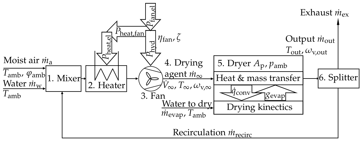
The following outlines the process path of the dryer shown in Figure 1:
- 1.
- The mass flow of water and moist air at ambient temperature , relative humidity and pressure as well as the recirculated mass flow , are mixed to reach the desired mass fraction of water vapor and mass flow of the drying agent.
- 2.
- The mixed flow is heated by an electrical heater to reach the desired temperature of the drying agent. The input energy is corrected by heat generated from turbulence heating from the fan.
- 3.
- The fan supplies the hydraulic power necessary to achieve the desired volumetric flow , taking into account pressure losses from free jets, flow around corners, filters, mixers, and other components, summarized in the pressure loss coefficient . The necessary electrical power with consideration for the electrical to hydraulic efficiency of the fan .
- 4.
- The drying agent is defined by three parameters: mass flow , temperature , and vapor mass fraction .
- 5.
- The drying agent enters the dryer, heats and evaporates water until a fraction of the thermal equilibrium is reached. The water mass flow to be dried is calculated using the drying rate and the product area .
- 6.
- It should be noted that only a fraction of the output flow can be recirculated into the mixing step. The remaining fraction is the exhausted mass flow .
2.2.1. Evaluation Criteria
The analysis of the dryer system is based on three key factors. Firstly, the SEC (Eq. 1) describes the electrical power added to the system per unit mass flow of evaporated water
Lower values indicate a more optimal operation point.
Secondly, the normalized drying power is introduced (, Eq. 2), which includes the temperature-dependent enthalpy of vaporization
Higher values indicate more favorable operation points. For the system under investigation, the scale ranges from "0," representing no evaporation, to "1," representing complete energy expenditure due to evaporation.
Thirdly, the evaporation potential (EP, Eq. 3) quantifies the mass of water that can be evaporated per unit mass of drying agent
This provides a theoretical upper limit on the usability of the drying agent for evaporation.
2.2.2. Evaporation Potential
The EP is calculated by solving a coupled mass and energy balance. The mass balance equation (Eq. 4) is based on the assumption that the air is saturated. It should be noted that this assumption restricts the saturation temperature to the boiling temperature . It is important to note that the drying agent and the wet surface are in thermal equilibrium. In light of these considerations, the EP describes the upper boundary of evaporation of the drying agent. The saturated moisture load is described by two terms: First, the water vapor mass per air mass, and second, the air saturation
The water vapor mass flow in the drying agent , and the maximum evaporation mass flow describe the water mass flow. The air mass flow is described by . The molar masses of water and air are multiplied by the saturation vapor pressures at the saturation temperature , also considering the ambient pressure . The equation can be rearranged to calculate the maximum evaporation mass flow . It is calculated as a function of saturation temperature
If pure water vapor is considered as the drying agent, the saturation temperature can be calculated using the inverse formulation of the vapor pressure at ambient pressure . In this case, only the energy balance needs to be solved (Eq. 5).
The energy balance considers thermal equilibrium in a stationary state. The reference temperature for zero enthalpy of dry air and liquid water is established at , aligning with the standard definition found in most Mollier diagrams. Note that the temperatures indicated in Eq. 5, 6 and 10 are expressed in }. To ensure consistency and accurate calculations, it is essential that the enthalpy is set to zero at the reference temperature .
The energy balance for the drying agent is described in two terms, the inflow enthalpy flow at the nozzle and the saturation enthalpy flow
In this segment of the flow changes temperature while drying.
The energy balance for the water to dry is also described in two terms: The inflow enthalpy flow as liquid water and the evaporated enthalpy flow
In this segment of the flow changes temperature and phase while drying. The energy balance of the enthalpy flows is achieved when the sum of the inputs is equal to the sum of the outputs
The quantity of interest is the saturation temperature . The explicit solution of the balance is displayed in Eq. 5
The specific heat capacities of the air component in the drying agent and at saturated state as well as the specific heat capacities of the water vapor component in the drying agent and the saturated state together with the heat capacity of liquid water have an influence in the equation. The heat capacity of water vapor is dependent on temperature and partial pressure. The heat capacity of air is dependent on temperature. The heat capacity of water is constant.
2.2.3. Partly Evaporation Potential
The optimal drying process considers thermal equilibrium of flow and wet surface leading to the maximal possible evaporation mass flow . In technical applications, the exchange heat and mass between the drying agent and the wet surface is constrained by the exchange coefficients and length scales of the dryer. To determine the amount of utilized EP, we define a evaporation potential fraction , which is calculated by
This quantity can be used as a calculation parameter or calculated by the evaporated mass flow (see Eq. 9). This mass flow is directly proportional to the drying rate and the area of the product surface exposed for exchange
The area of exchange for a quadratic round nozzle field (RDF) can be described by the spacing and the number of nozzles , as illustrated in Figure 3.
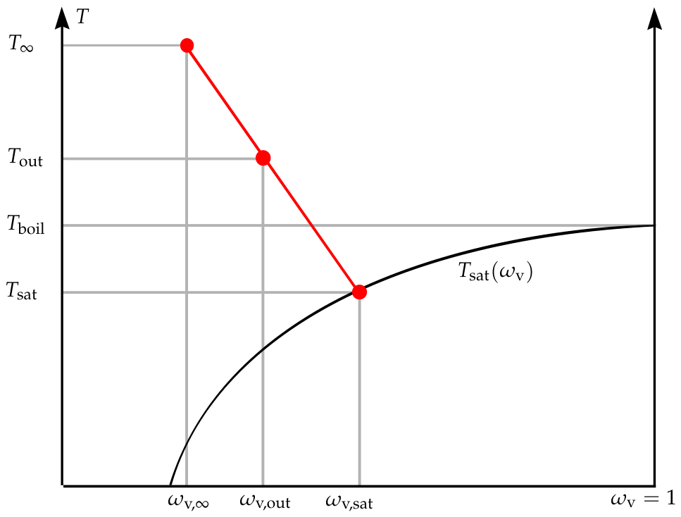
The drying rate is calculated using Eq. 18. To solve for the corresponding outflow temperature , an additional energy balance (see Eq. 10) is derived. As water evaporates from the wet surface, the drying agent cools down, converting sensible heat into latent heat. If the full EP is utilized, the drying agent cools to the saturation temperature . When only a fraction of the EP is used, the drying agent cools less. The outcome of this process is an outflow temperature that falls between the drying agent temperature and the saturation temperature . The specific heat capacities of vapor and air at the outflow temperature are and respectively.
The outflow temperature (Eq. 10) can be calculated using the same equations as Eq. 5 and substitute for and for . The reason for this difference is that only the equation for the outflow enthalpy flow differs from the saturation enthalpy flow in these variables
So, the resulting equation for is Eq. 10
The different combinations of temperatures and water vapor mass fractions are displayed in Figure 2.
2.2.4. Equations of Components
The components displayed in Figure 1 are calculated as indicated in Table 1. The drying agent (4.) is defined by the operation point that is the subject of the investigation.
The total mass balance at the mixer (1.) is solved by Eq. 11
The recirculation system’s water mass flow rate is set to 0 kg/s. The non-recirculation system’s recirculation mass flow rate is set to 0 kg/s.
The air mass balance is described in Eq. 12
The energy balance (Eq. 13) at the mixer is
The enthalpy of the flow at the nozzle is calculated as the sum of three terms: The input enthalpy from the mixing step , the turbulent heating , and the power added from the heater
The outflow enthalpy (Eq. 15) is the sum of the air and the water vapor enthalpy
The dissipation of hydraulic power into heat is a consequence of turbulence. It is assumed that the heating from turbulence is negligible for the density of the drying agent before and after the fan. Consequently, the density can be estimated as equal at the fan and the nozzle . The heating power (Eq. 14 and 16) can be calculated in advance. The power required for the fan to achieve the desired volume flow with the corresponding pressure drop can be calculated by
The total electrical power used is calculated in Eq. 17 as the sum of the electrical power of the heater and for the fan
The equations for and are displayed in Table 2.
2.3. Coupled Heat and Mass Transfer
Section 2.2 provides a description of the dryer system and the resulting normalized drying power (also the SEC considering 2) from a given drying agent and dryer configuration. This section will investigate the influence of the drying agent on the drying rate. The drying rate at an impermeable wet surface can be calculated using Eq. 18
which is also used in references [13,14]. The mass transfer coefficient is described in more detail in Section 2.4. is the universal gas constant; the surface temperature; the vapor pressure of the drying agent; and the vapor pressure at the surface. The gas layer above the wet surface is considered to be saturated air at the surface temperature . This assumption is false for porous media with reduced water vapor pressure due to capillary condensation according to the Kelvin-Law, or for surfaces that are already dry. The Stefan correction for mass transfer is implemented in Eq. 18 (see [14]). Drying can be considered a case of one-sided diffusion: while the water vapor diffuses from the surface, air cannot diffuse into the it. There is a partial pressure difference of air from outside the boundary layer to the surface. Therefore, air must have an overlaying diffusion flow, as described in [13]. This effect is accounted for in the Stefan correction.
The water vapor saturation pressure as a function of temperature (see Eq. 19) can be calculated using the Tetens approximation [15]
This formulation is accurate to from 0 °C–100 °C. Additionally, the formula can easily be inverted into . So the saturation temperature can be calculated using the flow conditions (see Eq. 6) at the nozzle or by knowing the saturation vapor pressure . Here, the temperature is inserted in } and the saturation pressure is calculated in }.
The unknown surface temperature is calculated using energy conservation (see Eq. 20) without heating the medium or considering radiation heat flux
Neglecting heat radiation can lead to errors in heat transfer. The radiation heat flux is negligible if the product is exposed to an area of similar surface temperature and the hotter area is relatively small. Similar assumptions are used in [16] and [17]. As a result, the convective heat flux is equal to the evaporative cooling heat flux , as shown in Eq. 20.
The convection term is corrected by the Ackermann correction factor , which accounts for the change in the boundary layer due to evaporation (compare Eq. 21 from [16], based on [18])
Since the evaporating mass flow is colder than the drying agent, it increases the thickness of the boundary layer, which decreases heat transfer and results in a correction factor smaller than unity . The heat transfer coefficient is described in more detail in Section 2.4. The specific heat capacity of water vapor at the surface also influences the Ackermann correction factor .
2.4. Dimensionless Formulations
The dimensionless formulation for impingement flow in a quadratic RDF from [21], based on [22] for turbulent flow, is used to estimate the convective heat transfer coefficient . See Figure 3. This formulation estimates the integral mean heat transfer for a moving surface under the nozzle field. To estimate the mass transfer coefficient , the heat and mass transfer analogy is employed.
Figure 3.
Quadratic RDF investigated in this work, compare to [21].
Figure 3.
Quadratic RDF investigated in this work, compare to [21].
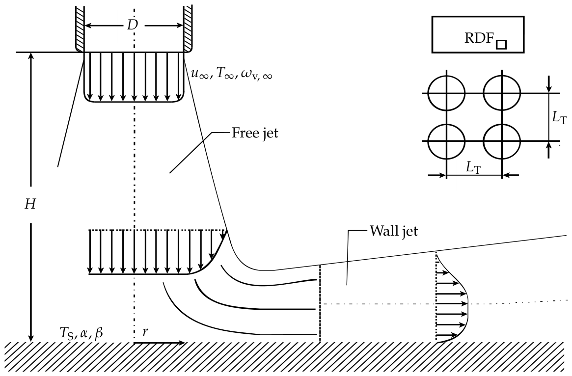
The dimensionless formulations for heat transfer and are used. The thermal conductivity and diffusion coefficient are dependent on temperature and vapor concentration and are evaluated at the film temperature and film vapor pressure . The nozzle diameter D, height H and pitch are geometric influence parameters. The limitations of the heat and mass transfer equations defined in [21] also apply here.
2.5. Flow Constants
It is not straightforward to compare the drying rates of different drying agents. Mixed gases have concentration- and temperature-dependent material properties . These are calculated using the equations and mixing rules from [21]. Even when considering the dryer’s geometric properties to be constant , the system remains underdetermined. The closing variable is the flow velocity at the nozzle . This is defined based on which parameter stays constant when comparing the drying rates of different drying agents. Different comparison cases have been evaluated in the literature (e.g., [16] volume and mass flow; [17] volume, mass flow, and Reynolds number).
2.5.1. Constant Hydraulic Power
In this work, we include the case of constant hydraulic power because it can be relevant for operators changing the operating point in existing plants. This ensures that the equipment, such as the frequency converters, electric motors, and fan drive trains, are suited for the new operating point and do not exceed their power specifications. However, the suitable temperature, rotational speed, and torque must still be verified.
2.5.2. Summary of Flow Constants
The following is a summary of the investigated flow constants:
- 1.
-
Constant volume flow (23)In this case, the rotational speed of the fan must not be adjusted for the dryer. Although the drying agent’s density changes, as well as the pressure drop and hydraulic power, the flow speed remains constant.
- 2.
-
Constant Reynolds-Number (24)In this case, the flow regime remains constant.
- 3.
-
Constant mass flow (25)In this case, the mass flow rate remains constant. An increase in temperature and moisture content results in a decrease in density and an increase in flow velocity.
- 4.
-
Constant hydraulic power (26)As mentioned above, the hydraulic power may be of interest to existing plants and their operators.
2.6. Numerical Solver
Solving the coupled heat and mass transfer functions (see Eq. 18 and 20) has the following limitations:
- The resulting surface temperature must be above the freezing temperature. To meet this constraint, a minimum moisture level in the system is required. Here was chosen.
- The material properties of air and vapor must be approximated. These approximations are performed for all concentrations and temperatures up to .
Figure 4 shows the solution steps.
3. Results
The following findings are investigated based on the methods explained above:
- 1.
- 2.
- In the cases of recirculation, the external water mass flow is set to zero for maximum recirculation and the internal recirculation mass flow is set to zero for no recirculation. In this study, the normalized drying power (see Eq. 2) is investigated. It describes the fraction of energy used for evaporation in reference to the supplied energy.
- 3.
- The influence of limited heat and mass transfer is shown for cases of fixed evaporation potential fractions (see Eq. 8).
- 4.
- The influence of fan power (see Eq. 16) is investigated by using various pressure drop coefficients .
- 5.
- As well as the combined influence of the limited heat and mass transfer and fan power.
3.1. Ideal Dryer
The EP (see Eq. 3) is calculated from equations 4 and 6 and is shown in Figure 5. The saturation temperature is shown in Figure 6. No data were calculated for drying agents below the saturation moisture line (solid black) or below the minimum water vapor mass fraction of the ambient air. As temperature increases, EP also increases. For superheated steam, this incline is steeper than for dry and moist air. The saturation temperature depends strongly on vapor mass fraction and slightly on temperature. These findings form the basis for the two adjustments made for non-ideal dryer systems.
3.2. Non-Ideal Dryer
3.2.1. Influence of Recirculation
This section investigates the influence of recirculation on the system. As stated in the literature, recirculating the used drying agent improves the overall SEC and normalized drying power. Table 2 shows the calculation parameters used. Figure 7 (left) illustrates the normalized drying power in a system that does not recirculate the used drying agent. In a system without recirculation, a higher vapor mass fraction of the drying agent results in a steep decline in normalized drying power due to the energy required to vaporize the water before it enters the dryer. Figure 7 (right) shows the normalized drying power in a system that recirculates the maximum amount of used drying agent. However, this is not the total flow amount because the added water vapor from drying must be removed by exhaust. In this system, the normalized drying power increases slightly with a higher water vapor fraction of the drying agent. The higher the water vapor fraction, the greater the amount of used drying agent that can be recirculated.
3.2.2. Influence Evaporation Potential Fraction
If only a fraction of the EP is used multiple things change regarding the normalized drying power and one quantity stays constant. The results for different cases of are displayed in Figure 8. The optimal operating point is superheated steam at a normalized drying power of . For an ideal case of this value constant for all temperatures, for cases the boiling temperature is ideal and higher temperatures are less efficient. The optimal operating point for dry air drying behaves differently. Its normalized drying power decreases with decreasing . For dry air drying the optimal operating point is always at the highest possible temperature.
3.2.3. Influence of Fan Power
When the fan power is a significant portion of a system’s total power usage, drying agents with a low EP have a lower normalized drying power. Figure 11 shows the results of various pressure loss coefficients values for the drying systems. While a value of represents the edge case of one dynamic pressure loss, technical systems with filters and multiple bends can achieve values even higher than [21], where translates into K using .
The heat from the fan can exceed the heating required by the heater at the investigated operating point. This is particularly true for design points involving low temperatures, high moisture, and high pressure drops. In these cases, the heater acts as a chiller to reach the desired temperature . The energy required to chill the flow is provided by heat exchange with the environment. Therefore the power for the heater is set to zero for Eq. 17. The line where the heater power is is displayed as a dotted line. Operating points with higher temperatures or lower moisture above the line have positive heater power, operating points below have zero heater power.
3.2.4. Combined Influence
As shown in Figure 12 and Figure 13, systems with significant pressure drop coefficients and non-equilibrium drying generally exhibit optimal behavior at intermediate temperatures with superheated steam. This analysis demonstrates that dryer systems have a well-defined optimal operating point. This point is never at an extreme of the temperature operating range. In Figure 13 an exception is shown for the case of constant mass flow. Higher water vapor mass fractions and higher temperatures decrease the density of the flow. However, velocity increases to maintain a constant mass flow, which leads to a significantly greater pressure drop and requires more hydraulic power. In this case, the power required for the hydraulic fan is greater than the power needed to heat the flow to the desired temperature. Since the fan’s heating is less efficient than the heater’s, an operation point with higher density is preferred over optimal recirculation.
The quantity of the calculations in Figure 12 changes based on the flow velocity at the nozzle , as calculated in Section 2.5.2. In all cases, the optimal operating point is superheated steam. Figure 14 displays the dependency of the normalized drying power on the flow velocity .
3.3. Heat and Mass Transfer
After extensively investigating the optimal operating point of the dryer, the influence on the drying dynamics must be considered, such as the process parameter drying rate. The literature has investigated cases involving constant volume flow, mass flow, and Reynolds numbers. However, the operator may be more interested in comparing points of the same hydraulic power, so this reference has been added to this work. Figure 9 shows the drying rates of the investigated cases.
Notably, the drying rates of dry air () and superheated steam () are equal at one specific temperature, that called the inversion temperature . For temperatures lower than the inversion temperature, dry air has higher drying rates. Temperatures higher than the inversion temperature result in higher drying rates for superheated steam.
The drying rates of the investigated cases are also analyzed (see Figure 15). For the four comparison cases, a clear inversion temperature of occurs for constant mass flow. Cases with constant volume flow do not show an inversion temperature, and it is unclear if one will occur at higher temperatures. An inversion temperature may occur slightly above for cases of constant hydraulic power and constant Reynolds number. A wide range of mass flow, volume flow, hydraulic power and Reynolds number was tested without significantly affecting the inversion temperature.
4. Discussion
4.1. Revision of Assumptions
First, the assumptions made for the ideal dryer system in Section 2.2 are critically revisited:
-
No product influenceIn industrial applications, there is always a product that needs to be dried. This assumption is justified if the product has high moisture content, low heat capacity, significant first drying stage behavior, and no constraints regarding flow or temperature. This may apply to thin products, such as paper, or shapeless gels. The influence of thick products, such as calcium silicate slaps, is currently under investigation. Further work will investigate how material parameters (see [23]) influence the optimal operating point. Drying models (see [24]) will be used to calculate the heat and mass exchanges () with the product.
-
Stationary stateStationary operation is possible for continuous belt dryers used in industrial applications. Smaller dryers with significant ramp-up and ramp-down phases are not considered here. Additionally, a significant number of dryers are operated in batch mode, which is not accounted for in this model.
-
Impermeable and adiabatic boundariesThe impermeable boundaries of the dryer may limit the applicability of the ideal model. As shown in Figure 7, recirculating the flow is especially important for superheated steam operation points. Real continuous belt dryers exchange with the atmosphere at the product’s inlet and outlet. The amount of lost drying agent flow or added atmospheric flow depends strongly on the configuration. Modern dryers use heat-up and cool-down zones at the product inlet and outlet, which reduces the exchange.Considering the dryer’s adiabatic boundaries only applies to well-isolated configurations. Insufficient isolation increases heat transfer through the wall, lowering the wall’s internal temperature and the heat in the recirculated flow. To approximate the heat transfer through the wall, the heat transfer coefficients inside and outside the dryer must be estimated. The thermal conductivity of the wall is easier to calculate. The surface area of the dryer will be problematic. Therefore, the length must be known, which depends on the belt velocity, drying rate, and moisture to be removed. Coupling these effects and influences will be addressed in future work but is beyond the scope of this paper.Lower wall temperatures can lead to condensation on the wall, which decreases the moisture in the recirculated flow. For superheated steam applications, this effect is critical because the energy lost by condensation must be supplied by the heater. Additionally, higher water vapor mass fractions lead to higher dew point temperatures, which increases the temperature limit for wall temperature.
-
Homogeneous flowThe assumption of homogeneous flow can be validated for real configurations through computational fluid dynamics analysis or measurements. Typically, mixing the flow is achieved through additional constructive measures. The homogeneous distribution to the nozzles is also considered.
-
Only convection consideredAs mentioned previously (see Section 2.3), we consider heat transfer to be dominated by convection. Although radiation increases significantly with higher temperatures, it is considered small due to the low area of high-temperature surfaces surrounding the evaporation surface. If we were to consider radiation, the radiation heat flux would be added to the convection heat flux to match the evaporation heat flux (see Eq. 20, which is valid for the first stage of drying). The added heat would result in higher drying rates, but the effects on surface temperature and dryer performance must be analyzed carefully.
4.2. Findings from the Results
Using the ideal and non-ideal dryer models, we found several results:
-
RecirculationCalculations show that recirculation of used drying agent can increase the energy used for evaporation of water while drying. The increase in efficiency is highly dependent on the amount of drying agent circulated, as efficiency drops significantly without circulation. That is because providing moisture by direct evaporation from environment and not from the evaporation consumes a lot of energy. Therefore, a good strategy is to keep the vapor inside the system by recirculating it.
-
Evaporation potentialThe EP defined in this paper establishes a theoretical upper limit for convective heat and mass transfer processes based on first principles. This limit depends only on the temperature and vapor mass fraction of the drying agent.
-
Drying rateThe drying rate is calculated for different cases (see Figure 9). If the operating point of the dryer changes, the changes in the drying rate must also be considered. If the dryer is of fixed length, the production capacity may also change because the belt velocity must be adjusted. In future work, we plan to incorporate the drying rate more specifically into the model by considering its effects on the belt velocity, dryer length etc. Additionally, we plan to incorporate heat loss through conduction over the dryer walls, considering the significant role of the wall surface area. This will allow us to more closely integrate the drying rate into the dryer performance calculations.
-
Evaporation potential fractionThe defined evaporation potential fraction provides an estimate of the effectiveness of the heat and mass transfer. Depending on the comparison case (see Figure 10), the value can differ significantly or slightly within the investigated domain. Further work is needed to evaluate whether this quantity can be used to estimate the drying rates of heat and mass transfer systems without knowledge of the dimensionless transfer functions.
-
Fan influenceThe analysis of the fan influence (see Figure 11) revealed that drying agents with small EPs are not ideal for achieving optimal operating points. In these cases, moving the fluid results in significantly higher energy consumption compared to the evaporated mass. This effect favors drying agents with higher temperatures. Additionally, it was shown that the heat from turbulence dissipation can raise the temperature of the fluid above that of the desired drying agent. In these cases the heat must be dissipated. At high hydraulic powers, this effect favors drying agents with low to medium water vapor mass fractions.
-
Combined influence of fan power and limited transfer coefficientsThe combined influence of fan power and limited transfer coefficients results in a single optimal dryer operating point (see Figure 12 and Figure 13). This implies that the previous considerations mentioned in Section 2.2 have shortcomings in their suggestions for optimal dryer operating points. In our case, the optimal operating points are SSD at temperatures ranging from 105 °C–200 °C. Figure 14 shows that increased flow velocities reduce dryer efficiency. The optimal operating point shifts to higher temperatures as flow velocity increases due to higher evaporation mass flows and lower pressure drops from lower water vapor density.An exception occurs when the hydraulic power required for the desired mass flow rate at higher pressure drop coefficients exceeds the heater power. See Figure 13 for a constant mass flow rate. In this case, the optimal operating point shifts away from SSD to moist air drying.
-
Inversion temperatureThe inversion temperature has been investigated in the literature, as well as in this work. It is a byproduct of investigating the optimal operating point of the different comparison cases with limited heat and mass transfer coefficients. While this quantity is of interest for academic considerations and drying rate optimization problems, it of minor importance for determining the optimal dryer operation point.
5. Abbreviations, Variables and Subscripts
The following abbreviations, variables and subscripts are used in this manuscript:
| Abbreviations | |
| SSD | Superheated steam drying |
| RDF | Round nozzle field |
| Variables | |
| A | Area [m2] |
| a | Thermal diffusivity [m2/s] |
| D | Diameter [m] |
| Evaporation potential [−] | |
| f | Factor or function [−] |
| G | Geometry factor [−] |
| H | Height [m] |
| Enthalpy flow [W] | |
| h | Specific enthalpy [J/kg] |
| K | Resistance coefficient [−] |
| L | Length [M] |
| M | Molar mass[kg/mol] |
| Mass flow [kg/s] | |
| Nusselt number [−] | |
| n | Number [−] |
| P | Power [w] |
| Prandtl number [−] | |
| p | Pressure or partial pressure [Pa] |
| Heat flux [W/m2] | |
| R | Gas constant [J/(molK)] |
| Reynolds number [−] | |
| r | Radius [m] |
| Schmidt number [−] | |
| SEC | Specific energy consumption [J/kg] |
| Sherwood number [−] | |
| T | Temperature [°C] |
| u | Velocity [m/s] |
| Volume flow rate [m3/s] | |
| x | Moisture load of dry air [kg/kg] |
| Heat transfer coefficient [W/(m2 K)] | |
| Mass transfer coefficient [m/s] | |
| Diffusion coefficient [m2/s] | |
| Normalized drying power [−] | |
| Pressure drop coefficient [−] | |
| Efficiency [−] | |
| Thermal conductivity [W/(mK)] | |
| Kinematic viscosity [m2/s] | |
| Density [kg/m3] | |
| Relative humidity [−] | |
| Mass fraction [−] |
| Subscripts | |
| a | Dry air or air |
| amb | Ambient |
| boil | Boiling |
| case | Comparison case |
| conv | Convective |
| dryer | Dryer |
| el | Electric |
| EPF | Evaporation potential fraction |
| evap | Evaporation |
| ex | Exhaust |
| fan | Fan parameter |
| film | At boundary layer |
| heat | Heat or heater |
| hyd | Hydraulic |
| max | Maximal |
| mix | At mixer |
| nozzle | Nozzle |
| out | At outflow |
| p | Product or isobaric |
| recirc | Recirculation |
| ref | Reference |
| S | At surface |
| sat | At saturation |
| T | Pitch |
| uni | Universal |
| v | Water vapor or vaporization |
| w | Liquid water |
| Ackermann correction | |
| ∞ | At impingement nozzle |
Author Contributions
Conceptualization, H.P. and H.-A.J.; methodology, H.P. and H.-A.J.; software, H.P.; validation, H.P.; formal analysis, H.P. and H.-A.J.; investigation, H.P.; resources, H.P. and H.-A.J.; data curation, H.P.; writing—original draft preparation, H.P.; writing—review and editing, H.-A.J., S.A. and U.J.; visualization, H.P.; supervision, H.-A.J., S.A. and U.J.; project administration, H.-A.J. and S.A.; funding acquisition, H.-A.J. and S.A. All authors have read and agreed to the published version of the manuscript.
Funding
This research received no external funding.
Data Availability Statement
The original contributions presented in this study are included in the article. Further inquiries may be directed to the corresponding author.
Acknowledgments
We would like to thank Leander Hake, Jonas Herfurtner, Johannes Brundiers and the whole team of the laboratory of applied fluid dynamics and the FH Münster as well as Univ.-Prof. Dr.-Ing. habil. Uwe Jansoke from the University of Wuppertal for supporting us during this work. During the preparation of this manuscript, the author used DeepL Translator and DeepL Write for the purposes of translation and text editing as well as Google Gemini 3.1 Pro for supportive coding. Perplexity Pro and Scopus AI were used for supportive literature research. The authors have reviewed and edited the output and take full responsibility for the content of this publication.
Conflicts of Interest
The authors declare no conflicts of interest.
References
- Kemp, I.C. Fundamentals of Energy Analysis of Dryers. In Modern Drying Technology; Tsotsas, E.; Mujumdar, A.S., Eds.; Wiley, 2011; pp. 1–45. [CrossRef]
- Ares-Sainz, J.L.; Arias, A.; Feijoo, G.; Moreira, M.T. Toward the decarbonization of industrial drying technologies: Cross-sector sustainability, economics and efficiency integrated assessments with emphasis on the wood and paper Industries. Environmental Technology & Innovation 2026, 43, 105024. [CrossRef]
- Mujumdar, A.S. An overview of innovation in industrial drying: current status and R&D needs. Transport in Porous Media 2007, 66, 3–18. [CrossRef]
- Jafari, S.M.; Malekjani, N., Eds. Drying Technology in Food Processing; Elsevier, 2023.
- Çam, E.; Casanovas, M.; Moloney, J. Electricity 2025: Analysis and forecast to 2027.
- Da Silva, R.P.; Okeke, I.J.; Thirumaran, K.; Mosalpuri, M.; Samadi, F.; Nimbalkar, S.U.; Cresko, J. Current state and future projections of drying processes in the US food and pulp and paper sectors: Energy, economic, and environmental assessment. Energy Conversion and Management: X 2025, 27, 101181. [CrossRef]
- Shukla, P.R.; Skea, J.; Reisinger, A.R., Eds. Climate change 2022: Mitigation of climate change; IPCC: Geneva, 2022.
- Sulzgruber, V. Introduction of the drying toolbox: Theoretical potential for energy savings in drying processes, 2026.
- Zühlsdorf, B. Project 68 - Task 1 - Technologies - Yearly Report 2025, 2025.
- Kröll, K. Trocknungstechnik: Trockner und Trocknungsverfahren, 2 ed.; Vol. Band 2, Springer: Berlin, Heidelberg, 1978.
- Swasdisevi, T.; Devahastin, S.; Thanasookprasert, S.; Soponronnarit, S. Comparative Evaluation of Hot-Air and Superheated-Steam Impinging Stream Drying as Novel Alternatives for Paddy Drying. Drying Technology 2013, 31, 717–725. [CrossRef]
- Chryat, Y.; Romdhana, H.; Esteban-Decloux, M. Reducing energy requirement for drying of beet-pulp: Simulation of energy integration between superheated steam and air drying systems. Drying Technology 2017, 35, 838–848. [CrossRef]
- Krischer, O.; Kast, W., Eds. Trocknungstechnik: Die wissenschaftlichen Grundlagen der Trocknungstechnik, 3 ed.; Vol. 1, Springer-Verlag Berlin Heidelberg, 1978. [CrossRef]
- Vu, H.T.; Tsotsas, E. A Framework and Numerical Solution of the Drying Process in Porous Media by Using a Continuous Model. International Journal of Chemical Engineering 2019, 2019, 1–16. [CrossRef]
- Tetens, O. Über einige meteorologische Begriffe. Z. Geophys 1930, 1930.
- Schwartze, J.P.; Bröcker, S. The evaporation of water into air of different humidities and the inversion temperature phenomenon. International Journal of Heat and Mass Transfer 2000, 43, 1791–1800. [CrossRef]
- Volchkov, E.P.; Leontiev, A.I.; Makarova, S.N. Finding the inversion temperature for water evaporation into an air–steam mixture. International Journal of Heat and Mass Transfer 2007, 50, 2101–2106. [CrossRef]
- Heyser, A. Wärmeübergang und Stoffübertragung bei großen Partialdruckdifferenzen. Chemie Ingenieur Technik 1956, 28, 161–164. [CrossRef]
- Wikipedia. Empirical equation for vaporization enthalpy, 2026.
- Magnus, H. X Steam, Thermodynamic properties of water and steam, 2026.
- Stephan, P.; Kabelac, S.; Kind, M.; Mewes, D.; Schaber, K.; Wetzel, T. VDI-Wärmeatlas; Springer Berlin Heidelberg: Berlin, Heidelberg, 2019. [CrossRef]
- Hofmann, H.M.; Kind, M.; Martin, H. Measurements on steady state heat transfer and flow structure and new correlations for heat and mass transfer in submerged impinging jets. International Journal of Heat and Mass Transfer 2007, 50, 3957–3965. [CrossRef]
- Weber, L.; Paschert, H.; Jantzen, H.A.; Janoske, U. Measurement of moisture profiles in porous materials based on optical perception. Measurement: Sensors 2026, p. 102003. [CrossRef]
- Weber, L. Comparison of a heat-air-moisture model with experiments for the drying behaviour of gypsum boards at higher temperatures. In Proceedings of the Proceedings of the 35th European Modeling & Simulation Symposium, EMSS. CAL-TEK srl, 2023. [CrossRef]
Figure 1.
The configuration of the dryer is idealized, with recirculation and non-equilibrium drying. Each component is modeled numerically using the stated equations. The energy consumption of a given drying agent is calculated based on the parameters of the dryer.
Figure 1.
The configuration of the dryer is idealized, with recirculation and non-equilibrium drying. Each component is modeled numerically using the stated equations. The energy consumption of a given drying agent is calculated based on the parameters of the dryer.
| 6. Splitter |
| Exhaust |
| Output |
| Heat & mass transfer |
| Drying kinectics |
| 3. Fan |
| 2. Heater |
| 1. Mixer |
| Moist air |
| Recirculation |
| Water to dry |
| 4. Drying |
| agent |
| Water |
| , |
| 5. Dryer |
Figure 2.
The schematic illustrates the flow states at the nozzle, outlet, and saturation point. The drying agent with temperature enters the dryer at the nozzle with the water vapor mass fraction of . Its temperature decreases and its water vapor mass fraction increases. Once thermal equilibrium is achieved, the temperature reaches saturation temperature and saturation water vapor mass fraction . If the thermal equilibrium is not reached the flow reaches the intermediate outflow temperature with the water vapor mass fraction . For superheated steam () the saturation temperature equivalent to the boiling temperature at the specified pressure.
Figure 2.
The schematic illustrates the flow states at the nozzle, outlet, and saturation point. The drying agent with temperature enters the dryer at the nozzle with the water vapor mass fraction of . Its temperature decreases and its water vapor mass fraction increases. Once thermal equilibrium is achieved, the temperature reaches saturation temperature and saturation water vapor mass fraction . If the thermal equilibrium is not reached the flow reaches the intermediate outflow temperature with the water vapor mass fraction . For superheated steam () the saturation temperature equivalent to the boiling temperature at the specified pressure.
| T |
| T |
| T |
| T |
Figure 4.
Flowchart for solving the surface temperature and drying rate .
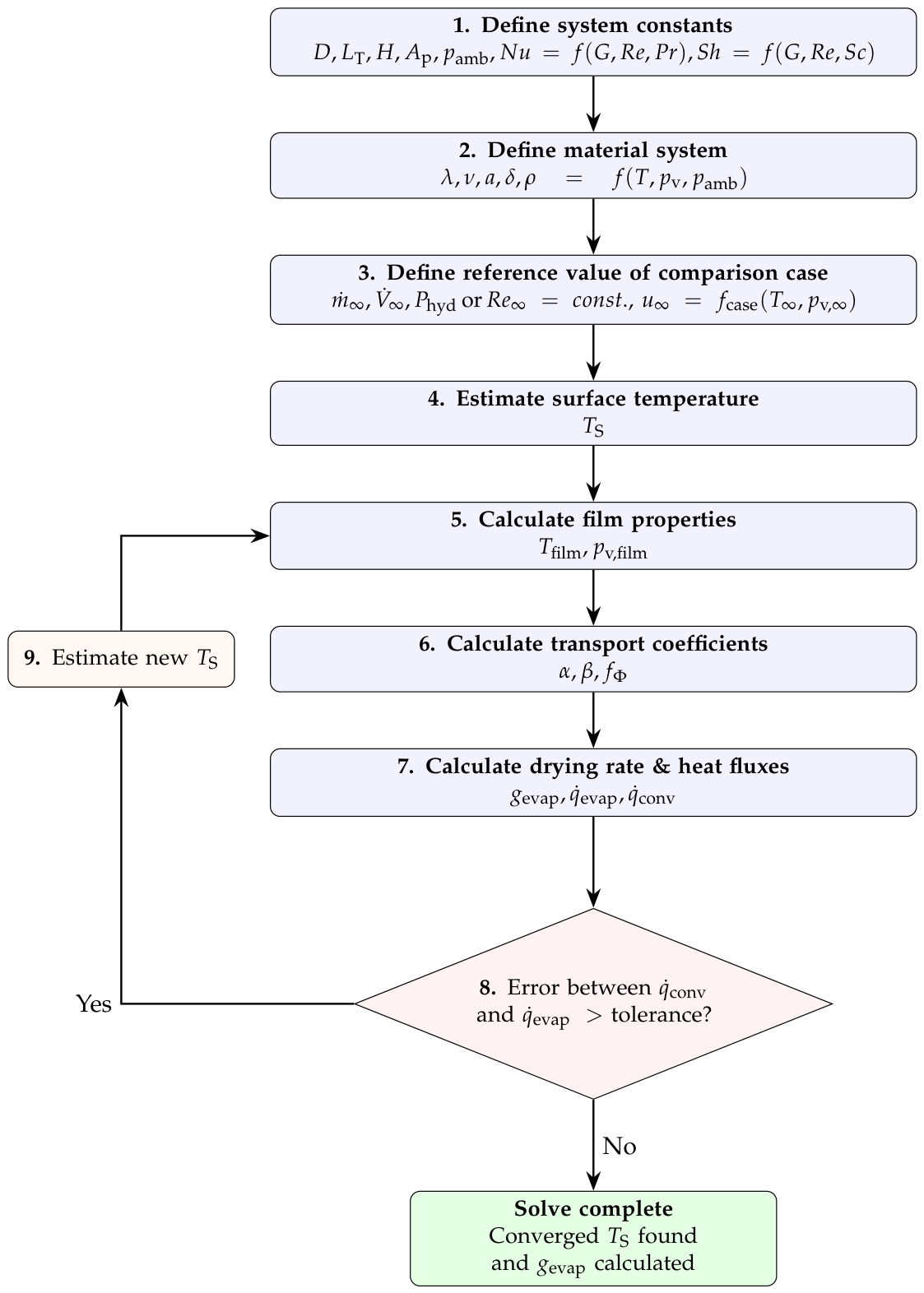
Figure 5.
EP is the amount of water that can be evaporated per unit mass of drying agent as a function of temperature and water vapor mass fraction. Superheated steam at high temperatures has the highest evaporation potential; saturated air has none.
Figure 5.
EP is the amount of water that can be evaporated per unit mass of drying agent as a function of temperature and water vapor mass fraction. Superheated steam at high temperatures has the highest evaporation potential; saturated air has none.
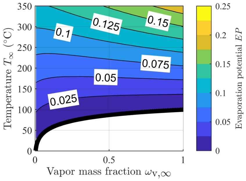
Figure 6.
The saturation temperature of the drying agent is a function of temperature and water vapor mass fraction. Low moisture air has quite low saturation temperatures, while high moisture air approaches the boiling temperature.
Figure 6.
The saturation temperature of the drying agent is a function of temperature and water vapor mass fraction. Low moisture air has quite low saturation temperatures, while high moisture air approaches the boiling temperature.
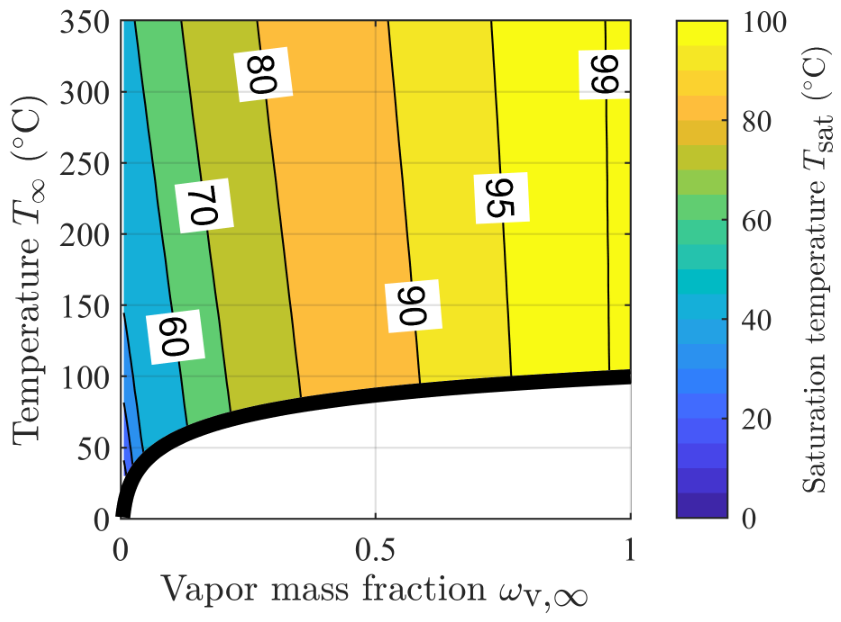
Figure 7.
Normalized drying power (see Eq. 2) (left) without and (right) with recirculating the flow. Recirculating the drying agent increases the normalized drying power. This effect is strongest with superheated steam.
Figure 7.
Normalized drying power (see Eq. 2) (left) without and (right) with recirculating the flow. Recirculating the drying agent increases the normalized drying power. This effect is strongest with superheated steam.
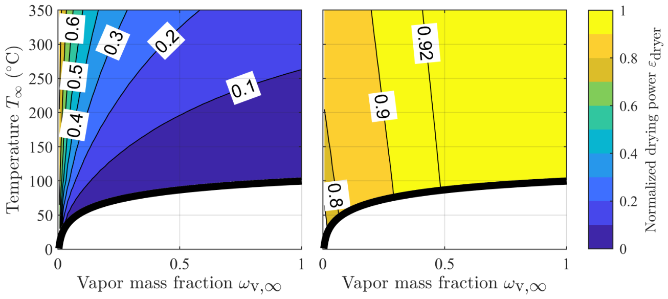
Figure 8.
Normalized drying power of the drying system with different evaporation potential fractions (top left) , (top right), (bottom left) and (bottom right). The optimal operating point is always at superheated steam at boiling temperature with a normalized drying power of .
Figure 8.
Normalized drying power of the drying system with different evaporation potential fractions (top left) , (top right), (bottom left) and (bottom right). The optimal operating point is always at superheated steam at boiling temperature with a normalized drying power of .
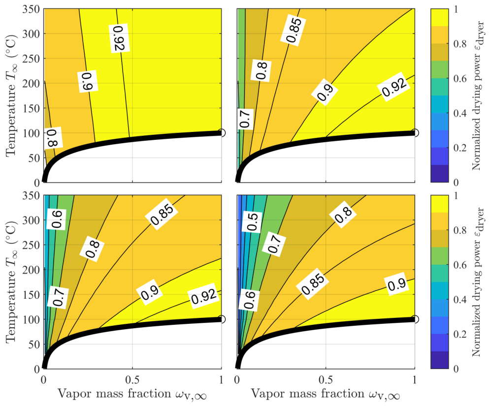
Figure 9.
Drying rates of different comparison cases (top left) , (top right), (bottom left) and (bottom right).
Figure 9.
Drying rates of different comparison cases (top left) , (top right), (bottom left) and (bottom right).
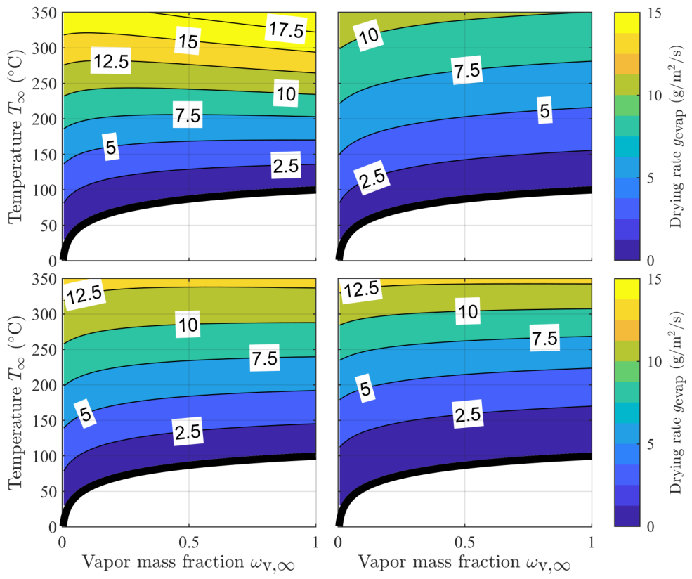
Figure 10.
The evaporation potential fraction is based on Eq. 8 for the comparison cases at (top left), (top right), (bottom left) and (bottom right).
Figure 10.
The evaporation potential fraction is based on Eq. 8 for the comparison cases at (top left), (top right), (bottom left) and (bottom right).
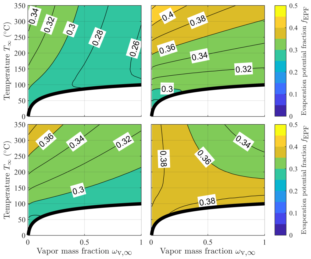
Figure 11.
Normalized drying power of the drying system for various pressure loss coefficients (top left) , (top right), (bottom left) and (bottom right). Drying agents with low EPs are inefficient for drying due to pressure loss from the flow. The dotted line indicates operating points with .
Figure 11.
Normalized drying power of the drying system for various pressure loss coefficients (top left) , (top right), (bottom left) and (bottom right). Drying agents with low EPs are inefficient for drying due to pressure loss from the flow. The dotted line indicates operating points with .
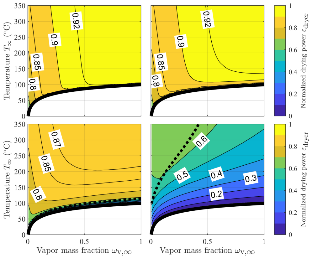
Figure 12.
Normalized drying power of dryer system with and constant value of: (top left) with , (top right) with , (bottom left) with and (bottom right) with . The dotted line indicates operating points with , here almost covered by the saturation line.
Figure 12.
Normalized drying power of dryer system with and constant value of: (top left) with , (top right) with , (bottom left) with and (bottom right) with . The dotted line indicates operating points with , here almost covered by the saturation line.
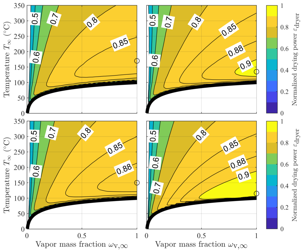
Figure 13.
Normalized drying power of dryer system with and constant value of: (top left) with , (top right) with , (bottom left) with and (bottom right) with . The dotted line indicates operating points with .
Figure 13.
Normalized drying power of dryer system with and constant value of: (top left) with , (top right) with , (bottom left) with and (bottom right) with . The dotted line indicates operating points with .
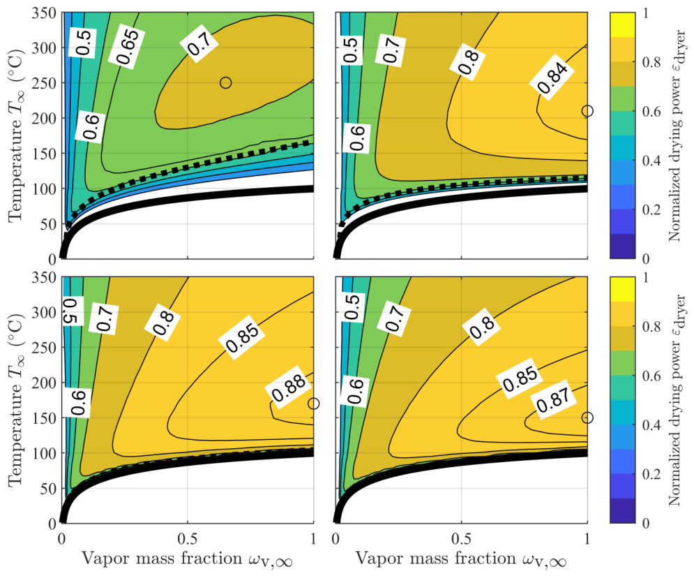
Figure 14.
Normalized drying power of dryer system with and at different flow velocities . The optimal operating points are marked and their quantities are displayed in the legend.
Figure 14.
Normalized drying power of dryer system with and at different flow velocities . The optimal operating points are marked and their quantities are displayed in the legend.
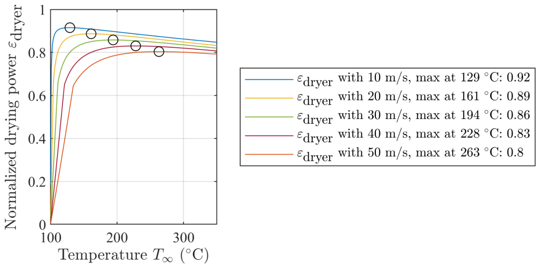
Figure 15.
Drying rate of different comparison cases for dry air and superheated steam (top left) , (top right), (bottom left) and (bottom right).
Figure 15.
Drying rate of different comparison cases for dry air and superheated steam (top left) , (top right), (bottom left) and (bottom right).
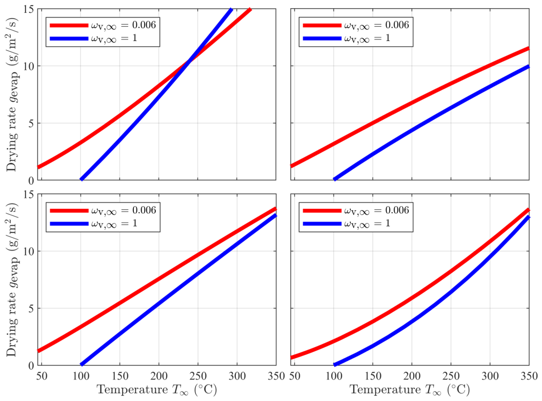

Table 1.
Calculation of dryer components.
| Component | Mass balance | Air balance | Energy balance | Power |
|---|---|---|---|---|
| 1. Mixer | Eq. 11 | Eq. 12 | Eq. 13 | W |
| 2. Heater | const. | const. | Eq. 14 | |
| 3. Fan | const. | const. | Eq. 16 | |
| 5. Dryer | const. | Eq. 15 | W | |
| 6. Splitter | const. | W |
Table 2.
Used parameters for calculation, compare to [10].
Table 2.
Used parameters for calculation, compare to [10].
| Parameter | Symbol | Value |
|---|---|---|
| Pressure loss coefficient | 0 | |
| Ambient temperature | ||
| Ambient rel. humidity | 80% | |
| Drying agent mass flow | 1 kg/s | |
| Nozzle diameter | D | 0.01 m |
| Nozzle spacing | 0.05 m | |
| Nozzle height | 0.08 m | |
| Product surface area | 2.5 m2 | |
| Ambient pressure | 101325 Pa |
Disclaimer/Publisher’s Note: The statements, opinions and data contained in all publications are solely those of the individual author(s) and contributor(s) and not of MDPI and/or the editor(s). MDPI and/or the editor(s) disclaim responsibility for any injury to people or property resulting from any ideas, methods, instructions or products referred to in the content. |
© 2026 by the authors. Licensee MDPI, Basel, Switzerland. This article is an open access article distributed under the terms and conditions of the Creative Commons Attribution (CC BY) license (http://creativecommons.org/licenses/by/4.0/).
Copyright: This open access article is published under a Creative Commons CC BY 4.0 license, which permit the free download, distribution, and reuse, provided that the author and preprint are cited in any reuse.