

Submitted:
08 October 2026
Posted:
09 October 2026
You are already at the latest version
Abstract
Phase transport specifies the change of phase along a path, but a predictor must also determine the path from initial data. We study this distinction in a conservative projector–connection model on the physical--observation dual-axis structure. A homogeneous two-mode reduction preserves the field equations, Gauss constraint, and energy, and has a global classical flow. Horizontal transport followed by a fixed analyzer gives a nonvanishing coherent readout on an invariant plane. With known parameters, no active input, and zero Gauss momentum, we derive a closed system of seven inner products for the planar branch. The Jacobian of the phase rate and its first six time derivatives has full rank at an explicit rational state, proving that seven is the minimal smooth predictive dimension on an open dense set. The initial phase is independent of these seven states. Near equilibrium, the linear observable motion reduces to two states; on a separate invariant family, internal motion leaves the phase constant. These results are placed in a protocol-dependent realization theory based on future phase increments. We also derive a background-dependent frequency law and the leading nonlinear phase coefficient. Signed perturbations and half-amplitude contrasts isolate the cubic contribution, while an explicit correction separates it from the cubic term introduced by coherent integration. Dynamic references and finite-window array processing illustrate the distinction between instantaneous alignment and phase prediction. All numerical examples are synthetic; the proposed physical tests require independent calibration of a device realizing the stated action and readout.
Keywords:
physical–observation dual-axis structure
; phase transport
; observation dynamics
; minimal realization
; nonlinear observability
; dynamic reference
1. Introduction
A phase reference is not determined by an instantaneous phase difference. In a moving array, for example, two processing branches may remain mutually aligned while their common response changes with orientation, channel properties, or processing weights. Converting one response to the other therefore does not, by itself, predict the phase that either will acquire next. That prediction requires the state of the system producing the response, including any velocity or internal memory that affects its future.
The physical–observation dual-axis structure (PODA) writes the formation of a record as a joint law
where X describes the physical state, S the objective observation state, and B the admissible joint domain [1]. The distinction concerns the roles of the two states in record formation; it imposes neither statistical independence nor dynamical decoupling. A coherent readout of F gives a complex response. On its nonzero domain, the phase transport fundamental equation (PTFE) is the differential law associated with [2]. The question considered here is what dynamics can supply the path entering this law, and how much of that dynamics an exact phase predictor must retain.
The geometric ingredients have established precedents. Interference compares complex amplitudes through their relative phase [3]. Parallel transport of spectral subspaces is generated by the projector commutator introduced by Kato [4]; geometric phase and its interpretation as holonomy were developed by Berry and Simon, with a nonadiabatic cyclic formulation due to Aharonov and Anandan [5,6,7]. We use these constructions without an adiabatic approximation. An important distinction throughout is between the locally exact phase form of a single nonzero scalar response and the generally curved connection associated with a moving response subspace.
Prediction introduces a second, dynamical question. Nonlinear realization theory identifies states through their input–output behavior, while observability relates their local distinguishability to derivatives of the output [8,9,10]. Smooth quotient maps and behavioral equivalence provide the appropriate setting for reducing a deterministic system without changing its future outputs [11,12]. We apply this viewpoint to phase increments. The resulting quotient is specific to a readout and its admissible controls: two states indistinguishable by one phase protocol need not be physically identical or indistinguishable by another measurement.
For a concrete model, we couple a fixed-rank response projector to an anti-Hermitian parent connection through a conservative action. Its curvature term has the usual Yang–Mills form [13]; the projector kinetic term and observation protocol specify the model studied here. A homogeneous two-mode reduction satisfies the parent equations, including Gauss’ law. On an invariant plane, a horizontal coherent lift and fixed analyzer yield a constant nonzero readout amplitude. The Gauss constraint and a common orthogonal mode symmetry then reduce the prediction problem to seven inner products. We derive their closed equations and exhibit an exact nonzero phase-derivative determinant. The matching upper and lower dimension bounds establish a seven-dimensional local minimum on an open dense set, rather than merely a convenient seven-state parametrization.
The same equations yield a second set of results: a background-dependent small-oscillation frequency, an explicit cubic phase coefficient, and a constant-phase family with nonstationary internal fields. A proposed experiment combines background scans with signed perturbations and a half-amplitude contrast. Since coherent integration itself produces cubic terms, the prediction is made at the level of the measured complex statistic, not only the instantaneous phase. Independent state characterization and calibration remain necessary to identify a physical realization of the model. The present numerical results establish properties of the specified equations and analysis procedure, not experimental evidence for that realization.
Section 2, Section 3, Section 4, Section 5 and Section 6 develop the dynamics and coherent readout. Section 7 and Section 8 establish the phase-behavior reduction and its local dimension. Dynamic references and finite-window measurements are treated in Section 9, Section 10 and Section 11; Section 12 and Section 13 derive the proposed tests. Numerical trajectories, exact calculations, and the extension to an independent phase load are collected in the appendices.
2. Response Geometry and Phase Evolution
2.1. Configurations, Initial Data, and Readout
On a smooth admissible domain , define
Here r is the coherent readout map and a local configuration. A second-order state consists of ; a regular Hamiltonian formulation uses momentum instead of velocity. We assume all manifolds are finite-dimensional, Hausdorff, and second countable, and all maps are smooth unless a lower regularity is specified [11].
Let N denote the complete dynamical state space, with configuration projection and response . When these states determine the subsequent motion, evolution takes the form
Any actuator, clock, or controller memory needed to determine the future belongs to . An external input is kept separate only when its time history is prescribed. We consider finite-dimensional realizations of this complete state.
2.2. The Phase Connection of a Nonzero Scalar Response
On , set
Locally, gives . The unnormalized response instead satisfies , so the normalization in Eq. (4) is essential.
On the phase principal bundle , let denote the transported phase coordinate. The PTFE is
The current response determines u, whereas is transported along the path. Their initial phase origins may differ; compatible transport preserves this difference as a constant group factor.
The connection is intrinsic to . A decomposition into and additionally requires a product neighborhood or a specified splitting of admissible tangent directions. On a constrained joint domain, the total differential on a physical tangent vector is independent of any ambient extension, even when its separate coordinate terms are not.
2.3. The Joint Initial-Value Problem
Theorem 2.1
(Response-compatible dynamical lift). Suppose Eq. (3) is locally well posed, g is at least , and the configuration trajectory lies in . Along that trajectory, define
Then the state, amplitude, and phase satisfy
Given the complete initial state, an initial phase, and the compatible amplitude , the solution is unique on each interval of nonzero readout and obeys
The amplitude remains compatible: .
Proof.
Since and , we have , with the second term purely imaginary. Its real and imaginary parts give the amplitude and phase equations. Direct differentiation shows that Eq. (8) satisfies the same initial-value problem. Uniqueness of the state flow and of the linear phase equation completes the proof. □
Integrating phase along the state flow therefore agrees with reading the response phase directly. The relative factor
is conserved. Equation (9) also provides a consistency check when the state and phase are integrated separately.
In admissible product coordinates,
The first term vanishes when the physical state is fixed. When it moves, velocities along both axes may contribute to the phase rate. A fixed observation configuration need not yield a fixed observation phase.
2.4. Phase Acceleration
Differentiating along a twice differentiable path gives
For and , the local coordinate expressions are
If the configuration itself satisfies , then . The explicit time derivative includes changes in external driving.
Equation (12) separates acceleration of the state from nonlinearity of the response. Even uniform configuration motion can change the phase rate through the second derivative of the response. This contribution is symmetric in the velocities. It is not a curvature term: contraction of an antisymmetric curvature tensor with vanishes.
2.5. A Fiber Criterion for Dynamical Reduction
The following standard descent criterion [11] will be used to distinguish a sufficient instantaneous readout from a state that carries its own evolution.
Theorem 2.2
(Projectability of a vector field). Let be a smooth surjective submersion and V a smooth vector field on N. There is a unique smooth vector field W satisfying
if and only if, for any two points in the same fiber,
For all local times on which both sides are defined, the flows satisfy .
Proof.
Necessity is immediate. Conversely, define by projecting V at any point of . Equation (14) makes the definition independent of that choice. Local smooth sections of the submersion imply smoothness of W, and surjectivity implies uniqueness. Uniqueness of ordinary differential equations gives the relation between the flows. □
For example, on the tangent bundle of an observation-phase circle, consider
The same phase can have different velocities , producing different futures . The present phase is not a sufficient state; the missing datum is its velocity.
The levels , , and retain response data, phase transport, and task-specific invariants, respectively [2]. A further dynamical reduction is possible only when the retained quantities satisfy the fiber criterion. In particular, equality of present phase need not imply equality of its rate.
3. Coupled Projector–Connection Dynamics
3.1. Action and Physical Assumptions
We now choose the dynamics that generate the observation path. The model consists of a response projector coupled to an anti-Hermitian connection, with a quadratic covariant kinetic term and a Yang–Mills curvature term [13]. This action is a physical assumption of the model; it does not follow uniquely from the joint-state structure.
Work on flat spacetime , with spatial volume , signature , and . Gravitational backreaction and additional matter sources are omitted. The periodic spatial domain makes the homogeneous reduction finite in volume without introducing boundary fluxes.
Let be a fixed-rank response projector and an anti-Hermitian parent connection. Define
Use for Hermitian matrices and for anti-Hermitian matrices. The parent action is
Fixed-rank orthogonal projectors form a single unitary conjugacy orbit. A potential depending only on one projector and invariant under all unitary conjugations is therefore constant on that orbit. Equation (17) adopts this case. Nontrivial interactions arise from spatial covariant gradients and the parent curvature. Device-specific covariant operators, matter couplings, and dissipation are not included in this conservative action.
The projector P describes the projective direction of a multicomponent response. It may depend on without retaining all information in s. If the fields are pulled back from the joint domain, P and must describe the same physical history. One varies either the parent variables or an independent set of reduced variables, not both as separate degrees of freedom.
3.2. Projector Momentum and Connection Evolution
Admissible projector variations have the form , with . The tangent projection of a Hermitian matrix is
Varying Eq. (17) gives
The projector equation determines the tangential acceleration; differentiating twice determines the normal acceleration. Write
After retaining the equation obtained by varying , choose temporal gauge . The equations become
The initial data must also satisfy
The last relation is Gauss’ law, obtained by varying the temporal connection before fixing the gauge. It constrains the initial data and is propagated by the field equations. This order of variation and gauge fixing is the usual constrained-Hamiltonian prescription [14].
The normal term is fixed by the differentiated projector constraint. The tangential term contains spatial covariant gradients that depend on the evolving connection. The fields must therefore evolve together, with initial data satisfying Eq. (22).
The projector motion can also be written as , where
The generator is the off-diagonal part, relative to P, of an infinitesimal unitary motion. Its commutator with P gives the projector velocity, whereas measures the physical kinetic energy. Writing the motion in first-order unitary form therefore does not remove its independent momentum.
3.3. Inertia Induced by the Parent Kinetic Energy
In temporal gauge and a chosen mode representation, let . Its time-dependent kinetic term is
Defining along the same parameter variations gives
If parameter derivatives are covariant, the inertia and response metric must use the same . For spatially varying modes, the volume factor is replaced by a spatial integral. When the connection also depends on s, its electric kinetic term contributes
These coefficients describe the kinetic energy in the chosen parametrization. Gauge redundancy and the Gauss constraint must still be treated before the parameters are used as independent dynamical states.
A single scalar response has . Its projector kinetic term therefore gives no inertia for the common phase, intensity, or other device parameters that leave P unchanged. Those degrees of freedom require the parts of the full action that actually depend on them. Equation (14) then determines which variables may be reduced further.
For a mode embedding , varying the substituted action gives . This is the parent Euler equation projected onto the retained variations. To obtain a solution of the full model, the omitted equations and constraints must also vanish. We verify that requirement for the homogeneous reduction below.
4. Homogeneous Two-Mode Reduction
4.1. Inertia and Interaction Potential
For a rank-one projector on a two-component complex response space, use the Pauli representation
All coefficients depend only on time. The Pauli representation identifies the projector with a unit vector and the two retained connection components with vectors . These vectors are coordinates in the internal matrix space.
Using and , we obtain
The expression for follows by replacing with . Ordinary spatial derivatives vanish, but the commutators retain nontrivial covariant gradients and curvature.
Write . Substitution into the parent action and integration over space give
The constant has been subtracted. Both inertias and both interaction terms follow directly from Eq. (17).
4.2. Momenta, Gauss Constraint, and Equations of Motion
Varying first gives
Now choose temporal gauge . Let , , and , with momenta , , and . The projector momentum is tangent to the unit sphere.
Tangential variation of and independent variation of in Eq. (32) give
The initial data obey
These initial data determine the projector and connection trajectories through Eq. (34). The normal term preserves unit length; the remaining accelerations arise from the common potential.
4.3. Consistency with the Full Parent Equations
Proposition 4.1
Proof.
Products, commutators, and time derivatives of homogeneous matrices remain homogeneous, so the equations generate no omitted nonzero spatial modes. Both the projector current and the connection commutators are traceless. The central field and its electric field therefore remain zero if initially zero. For the omitted third spatial component, and , so both sides of its Euler equation vanish.
The retained equations follow either by direct substitution into Eq. (19) or by admissible variation of Eq. (32). With and , they imply
Uniqueness with zero initial data preserves , and hence both the projector and tangency constraints. Finally,
The projector–connection terms cancel pairwise, as do the interactions between the two connection modes. The initial Gauss condition is propagated, so the temporal field equation remains satisfied. □
In particular, a vanishing parent connection is incompatible with a freely rotating projector in this source-free model. Gauss’ law would give , and the unit constraint would then force .
4.4. Energy and the Global Initial-Value Problem
Theorem 4.2
Proof.
The smooth polynomial vector field gives a unique local solution. Constraint preservation follows from the preceding argument and Eq. (37). Contracting each equation of motion with its corresponding velocity shows that the derivative of the potential cancels the change in kinetic energy, so . Nonnegativity bounds all velocities:
The vector remains on the unit sphere, while and grow at most linearly on finite intervals; for example, . No state component can escape to infinity in finite time, and the local solution extends to all real times. □
The argument proves global existence for this finite-dimensional homogeneous system. It makes no regularity claim for the spatially inhomogeneous field equations.
4.5. Nondimensionalization and Example Initial Data
The two inertias define the time and energy scales
With primes denoting , both normalized inertia coefficients in are unity. The dimensional quantities and nevertheless have different units. For the numerical example, take
The Gauss condition is exactly satisfied, but the initial state is not a stationary point of the potential. Equation (34) gives
Thus the response direction begins to move even though all initial velocities vanish.
5. Horizontal Coherent Transport and Phase Readout
5.1. Lifting the Phase Reference
A projector specifies a complex line, but not a phase on that line. We fix an initial unit representative and transport it horizontally. The projector-commutator equation below is Kato’s parallel transport [4], written with the parent covariant derivative. Unlike its use in an adiabatic approximation, its role here is to define an exact readout protocol along the trajectory.
Theorem 5.1
(Horizontal coherent lift of the projector). Let be a smooth rank-one orthogonal projector and set . Given and , the equation
uniquely determines a horizontal representative and preserves
For the global parent solutions of the preceding section, the lift is also global.
Proof.
Because is anti-Hermitian, the linear equation preserves the norm. The matrix satisfies , while the projector tangent identity gives . Their initial values agree, so uniqueness of the linear matrix equation yields . Finally, . The generator is bounded on every finite interval, allowing the linear lift to be continued. □
For a local normalized representative , set and . Then satisfies Eq. (43). Horizontal lifting thus removes the comparison phase of the local representative. Direct integration of the matrix equation avoids changes of formula at coordinate singularities of that representative.
5.2. Analyzer Readout and Its Second Derivative
Let be a calibrated unit analyzer in the same parent fiber. Define the normalized coherent readout by
Under a passive gauge transformation, and ℓ transform together to and , leaving invariant. Actual motion of the analyzer or a change in the electronic reference can alter the readout and must be retained as a state or a known input.
The parent equations determine , and the analyzer protocol determines . On each interval where , these quantities determine
and hence the first two time derivatives of phase.
In temporal gauge, with a fixed analyzer, the generator for Eq. (34) becomes
Substitution into Eq. (46) gives a complex-response evolution that can be integrated with the state equations.
5.3. Phase Acceleration Generated by the Interaction
For a fixed unit analyzer, let , so that , and set . Using , we obtain, for ,
The phase rate is therefore
Differentiation and substitution of Eq. (34) remove the normal acceleration through , leaving
The first term describes projector rotation driven by the parent potential; the second comes from the nonlinear analyzer response. Since the connection components also obey Eq. (34), the complete initial data determine the phase acceleration.
In general, this readout still depends on the complete state. One sufficient representation is
together with the analyzer reference and initial constraints. These data uniquely determine the parent trajectory and horizontal lift. Scalar phase is then continuous on each nonzero-readout interval.
5.4. Initial Phase Acceleration
Use the state in Eq. (41) and choose
In this subsection, primes denote derivatives with respect to dimensionless time . Define
Hence
The dimensional initial phase acceleration is . This analytic value checks the initial evolution independently of time integration.
With and , we also have
Cross-correlation of the two analyzer channels gives , in which the common lift phase cancels. It measures the relative phase between channels, whereas measures a single channel against the specified reference. They are distinct observables.
5.5. Path Memory and Scalar Flatness
Horizontal transport can carry path information not contained in the endpoint projector [6,7]. Retaining the representative , or its equivalent transport record, makes a single-valued scalar on the complete lifted state. Its phase form therefore satisfies
A closed projector path need not return the horizontal representative to its initial value. Such a history is not closed in the complete state space and is therefore consistent with Eq. (60). Viewed as a one-form on alone, Eq. (52) describes the projective geometry of horizontal transport, not the phase differential of a globally single-valued .
If the actual material response also contains a common amplitude and phase, write
The evolution of and then requires material equations or a physical reference. The dynamics above determine the specified normalized horizontal readout, not the common degrees of freedom absent from the projector.
Here is transported by the parent state without exerting a force on it. An independent conjugate phase load would require its own action and sources. Appendix E treats that different physical case.
6. Planar Dynamics and the Observable Phase
6.1. An Invertible Moving-Frame Representation
The homogeneous system admits an exact invariant plane. Coordinates that rotate with the response direction give a more direct relation between the parent dynamics and phase on this branch.
Fix the plane in the space of matrix coefficients. If and their initial velocities lie in this plane, the accelerations in Eq. (34) lie there as well. The dynamics preserve the restriction without an additional reaction force.
Define the response angle and moving unit vectors by
Write the two connection components as
Local observation-configuration coordinates for this realization are then
On a chosen angular chart, the inverse transformation is
The transformation retains the complete planar parent configuration, represented locally by . The initial coherent phase and continuous lift are handled as in Section 5.
The variables describe this dynamical branch; they do not redefine the entire observation axis through one readout. A physical device requires a formation map relating them to measurable parameters. In particular, is the angle of the response projector and is not a mechanical rotation angle unless calibration establishes that relation.
Planarity does not remove the parent curvature. Since ,
We also have and . Their matrix coefficients point normal to the internal plane, but the terms themselves are nonzero and contribute to the potential below.
6.2. Moving-Frame Inertia and Potential
The field velocity decomposes as
Applying the same decomposition to and substituting into Eq. (32) gives
The coefficients are unchanged from the parent action.
Set
In the coordinate order of Eq. (64), the full inertia matrix is
The sum of squares in the kinetic energy proves positive definiteness: zero kinetic energy first forces and then forces every remaining velocity to vanish. Equivalently, the Schur complement is . The full inertia remains nondegenerate even at . The connection kinetic term supplies precisely the directions absent from the projector term alone.
6.3. Equations of Motion and the Gauss Condition
Let
In these coordinates, the parent equations become exactly
The velocity terms involving arise from differentiating the moving frame; the remaining terms come from the parent potential.
The cyclic momentum is
Since , we have , while the other two Gauss components vanish identically on the plane. Independence of from makes conserved; the parent Gauss constraint requires its value to be zero. Substitution of Eq. (72) verifies
Thus is preserved. For configurations and velocities satisfying this condition, the moving-frame equations and parent equations determine the same trajectory.
Any planar vector initial data can be converted to coordinate initial data. For example,
The corresponding b relations use . This initial-data map allows the two representations to be solved independently and compared pointwise.
6.4. Constant-Amplitude Coherent Readout
Theorem 6.1
(Nonvanishing phase readout on the planar branch). For a planar parent solution, use the horizontal lift of Section 5 and the fixed analyzer . The normalized coherent readout satisfies, for all times,
Given the initial phase, its continuous lift is
Proof.
Phase acceleration is set by the products of the parallel and transverse components of the two connection modes. Those components evolve together under Eq. (72). The constant readout amplitude removes response-zero singularities from the phase coordinate on this branch.
The lifted angle also records the global phase reference: a increase returns the projector but changes the sign of the coherent representative, and a increase restores that factor. This is a property of the chosen horizontal readout along the angular path, not a statement that the full field trajectory is periodic [4,7].
6.5. The Observable Phase Mode Near Equilibrium
Consider a zero-potential equilibrium
where are background connection components. Set . Linearizing Eq. (72) gives
For example, the crossed contributions in the equation combine as . The restoring frequency is fixed by the action and background state.
The linearized Gauss constraint is
Together with and , this gives
Equivalently, . The two initial data for the phase rate form a closed state, while the initial phase is specified separately. This frequency refers to the chosen homogeneous representation and perturbation modes. A general spatial gauge transformation also changes the mode representation, so cannot be used independently of that convention.
For , define
Both modes oscillate at , but the first-order phase depends only on :
The phase retains the two initial data of the observable mode; the orthogonal mode has no first-order readout. At , the linearized Gauss constraint forces the phase rate to vanish identically. An internal restoring frequency still exists, but it does not appear as a nontrivial linear phase oscillation.
6.6. Analytic Prediction and the Nonlinear Remainder
Perturb the equilibrium (78) by taking , , , and zero initial velocities. The linear solution is
The initial value also holds exactly in the nonlinear system. Its subsequent cosine evolution is a linear approximation.
Changing the sign of leaves the equations invariant under and . Smooth dependence on initial data and the identity between the phase increment and imply, on a fixed finite interval ,
Reflection symmetry removes the even powers, and Eq. (84) gives the linear term. Near the initial time, the cubic coefficient is
The same result follows from in the full equations. For and sufficiently small perturbations, the nonlinear phase error on a fixed window scales as . Halving the perturbation therefore reduces the error asymptotically by a factor of eight. The estimate does not cover observation times that diverge as .
Linear oscillation does not imply stability of the full equilibrium. The parallel direction admits the exact drift , , , , satisfying both the parent equations and Gauss condition. An arbitrarily small c eventually carries the configuration away from the equilibrium while the phase remains constant. The fixed equilibrium is therefore not Lyapunov stable in the full configuration space, and the observable oscillation is not an attraction mechanism.
6.7. Internal Motion with Constant Phase
Proposition 6.2
(A nonstationary constant-phase family). Let and set
If
then these expressions define an exact solution of Eq. (72). The Gauss momentum vanishes identically, and both P and remain constant.
Proof.
Direct calculation gives and . Substitution into the parallel equations gives the equation multiplied by A and B; the transverse equations give the equation multiplied by B and . The antisymmetric products in Eq. (73) cancel pairwise. Both angular velocity and acceleration vanish, as do the horizontal generator and scalar phase rate. □
The family inherits the conserved energy
Its members can nevertheless have different gauge invariants, for example
Different values of thus give physically distinguishable internal configurations with identical prescribed phase histories. A readout of P alone cannot distinguish this family, since P itself remains fixed. Distinguishing its members requires a measurement sensitive to additional parent variables, or an intervention that couples those variables to the observed phase.
Observable linear oscillations and the constant-phase family distinguish the response state from the phase-prediction state. The former retains the full configuration producing the readout; the latter need only distinguish states with different future readouts. Section 8 determines the corresponding generic nonlinear local minimum.
7. Phase-Behavior Quotients and Minimal Dynamical States
The complete parent state determines future phase, but some state differences remain invisible to a given observation protocol. Retaining only the present phase, by contrast, discards velocity and reference motion. A minimal predictor must retain exactly those distinctions between initial states that lead to different future phases.
We use output equivalence in the sense of nonlinear realization theory [8,10], specialized to phase increments. Its relation to smooth behavioral quotients is particularly direct for deterministic systems [12]. The equivalence identifies prediction states for a protocol; it does not identify the underlying physical and observation states.
7.1. Future Phase Increments and Behavioral Equivalence
Let the input values lie in an open set , and let be a class of locally bounded, piecewise-continuous functions . Assume that the class contains every constant input and is closed under time shift and concatenation. The vector field and phase-rate function are smooth jointly in state and input. We assume a common forward-invariant state domain on which solutions exist uniquely for all and the readout is nonzero. A terminating observation can instead be modeled by including its termination time and status in the output; that extension is not needed here.
The state equation is
The response connection gives the phase rate
or an equivalent expression supplied by the chosen horizontal coherent protocol. Here is the configuration projection, and denotes the control input, not the unit-phase function of Section 2. Write the solution under a common input as and define the phase-increment factor
This group-valued factor starts at 1 and records future phase changes without selecting a branch of the real phase lift.
Definition 7.1
(Protocol-dependent phase equivalence). Fix a readout protocol and admissible input class . Two complete states are phase-equivalent under that protocol when
for every and all .
The relation compares increments, not phase origins. The initial phase is supplied separately; changing it multiplies the entire phase history by a constant group factor without changing the prediction state.
The phase-increment factor has a multiplicative cocycle property. If u is applied for time T and is followed by an input v, then
For equivalent initial states, the first factors on the right agree and are invertible. Equality of the concatenated histories therefore implies equivalence of the successor states. Thus a common input sends a behavior class to a uniquely defined behavior class. Equality of the group-valued histories is sufficient: their continuous real lifts, both initialized at zero, differ by a continuous integer multiple of and hence coincide.
Proposition 7.2
(Enlarging the input class refines equivalence). If , then
Internal states invisible under a passive protocol may therefore become distinguishable when active probing or further device controls are allowed.
Proof.
Indistinguishability under the larger input class implies indistinguishability under every subset. The converse need not hold. □
7.2. Minimality of a Regular Quotient
The set of behavior classes need not be a smooth manifold. The following result assumes that it is a regular quotient.
Theorem 7.3
(Dynamics and minimality of the phase-behavior quotient). Under the assumptions of this section, suppose the phase-behavior quotient is a smooth Hausdorff manifold and the quotient map is a surjective submersion. Then there are unique smooth functions and , jointly smooth in the reduced state and input, such that
with
and reproduce Eq. (93) exactly for every admissible input.
Let another realization consist of a smooth state equation , a smooth phase rate , and a smooth surjective-submersion initialization . Suppose this realization reproduces every future phase increment from under the same input. There is then a unique smooth map
Thus is the coarsest exact state distinction for this protocol; every other such smooth deterministic realization maps onto it.
Proof.
Fix an input value . Equation (95) makes constant on each fiber of p. A local section of the submersion defines the induced quotient evolution and shows that it is smooth. Differentiation at gives . The same section, chosen independently of a, establishes joint smoothness in state and input. For two states in one behavior class, differentiation of at zero gives the same phase rate; thus is well defined and smooth. The relations in Eq. (98) follow. For piecewise-continuous inputs they hold along trajectories almost everywhere, so the chain rule and integration recover the complete phase history.
If another exact realization satisfies , determinism requires identical phase histories under every admissible input. Hence . The map p is therefore constant on fibers of r and factors uniquely as . Local smooth sections of r make q smooth. □
The manifold and submersion assumptions are substantive. They need not hold across sets on which the behavior classes change dimension. Our concrete seven-state construction below establishes a local realization directly, without assuming a global smooth quotient across its singular sets.
With a local real phase lift , Eq. (97) reads
Phase prediction thus has two parts: a behavior state determining future increments, and a phase reference recording the current origin. For a nontrivial phase bundle, Eq. (100) is used locally and joined by transition functions; a global real phase is unnecessary.
7.3. Closure by Finitely Many Phase Derivatives
For an autonomous protocol with vector field V, output Lie derivatives furnish the local observability construction of Hermann and Krener [9]. Here the output is the phase rate, giving the candidate state
Proposition 7.4
(Closure and regularity of phase-derivative states). Suppose V and ν are smooth on an invariant domain and a smooth function G, defined on a neighborhood of the image of , satisfies
Then obeys the closed system
Together with an initial phase, this relation gives a sufficient prediction state. If is locally an embedded manifold, is a surjective submersion, and its fibers equal the phase-behavior classes, then is locally diffeomorphic to the regular behavior quotient. At rank r, its displayed components are independent local coordinates; otherwise coordinates must be chosen on the lower-dimensional image.
Proof.
Differentiation along the full flow gives Eq. (103). Equality of the fibers makes and the quotient map factor through each other. Their submersion properties make the induced maps smooth in both directions, giving a local diffeomorphism. Equality of fibers as sets alone would not ensure a smooth inverse. □
With control inputs, further differentiation of the phase rate generally introduces the inputs and their derivatives. These must be supplied as known external quantities or represented by actuator states in the complete system. Otherwise the derivative equations still lack information needed for evolution.
8. A Minimal Seven-Dimensional Nonlinear Phase Realization
Consider the full planar equations (72) with the fixed analyzer , horizontal coherent transport, known parameters, no external control, and zero Gauss momentum. Initial states are allowed to vary freely within the stated regular domain; in particular, their energy is not fixed in advance. A local phase realization means a smooth autonomous state equation, a smooth phase-rate output, and a smooth initialization map reproducing phase increments on the common local existence interval. Its dimension counts every variable needed for prediction, including any clock or conserved quantity not fixed in advance. The initial phase is supplied separately. We determine the minimum dimension in this class.
8.1. Gauss Reduction and Mode Symmetry
Collect like components of the two connection modes into two-dimensional vectors:
The vectors are the parent velocities resolved in the moving basis. Gauss’ law fixes the angular velocity algebraically:
Phase increments do not depend on the initial , so the initial angle and phase reference can be treated separately. Imposing one Gauss constraint and quotienting by initial-angle translation reduces ten configuration and velocity variables to four two-dimensional vectors. Differentiation gives
where , , and .
A common constant transformation of the four vectors preserves the equations, all inner products, and every phase increment. Its continuous orbit is one-dimensional on the regular domain below. The reduction consequently removes one further prediction-irrelevant direction. This is an output-preserving symmetry quotient, not a seven-dimensional symplectic quotient; fixing a momentum level and symplectic reduction are different operations [15].
8.2. The Seven-Inner-Product Flow
Define
In this section denote real inner products, not the background components of Section 6.5, nor the connections and . Since , the vectors form a basis. The remaining velocity inner products are reconstructed as
These formulas follow by inversion of the two-dimensional Gram matrix. Every seven-tuple with and is realizable. A smooth representative is
Equal values of the seven inner products give equal Gram matrices for , so a common orthogonal transformation relates the two bases. Inner products of with that basis then determine their images uniquely. The seven quantities therefore parametrize the mode-symmetry quotient on this regular domain.
Differentiating along Eq. (106) yields
The quantities are evaluated from Eq. (108); they are not additional states. Subtracting the equations for F and E gives
in exact agreement with the parent phase law. The energy becomes
The vector field is smooth and rational on . Given and an initial phase, it has a unique trajectory until it leaves this chart, reproducing the phase of the parent equations. This establishes a seven-dimensional upper bound. We next show that the dimension cannot be reduced near generic regular points.
8.3. Exact Phase Derivatives and Minimal Dimension
Apply Eq. (40): set , divide by , divide by , and divide the phase rate by . In the resulting variables ; denote the seven-dimensional vector field by f. The transformation is invertible and preserves differential rank.
To obtain a lower bound matching the explicit realization, use the output-derivative map from local nonlinear observability [9]:
Its components run from the phase rate through its sixth derivative, or equivalently from the first through the seventh derivative of phase.
Choose the realizable rational point
A representative is , , , and , with from Gauss. Exact differentiation gives
and
The determinant is the nonzero integer
The matrix is computed using rational time series and differentiation with respect to initial data. Its determinant is independent of floating-point rank thresholds. Appendix H gives the recurrence and reproduction procedure.
Theorem
(Local minimal dimension on the planar branch). For the fixed-analyzer, zero-input, known-parameter, zero-Gauss planar system, the domain , contains an open dense set on which the local phase-increment realization has minimal smooth dimension seven. Equations (107) and (110) supply such a realization near each point of this set. Its phase reference is an independent variable.
Proof.
The seven-inner-product flow supplies an output-preserving realization, hence an upper bound of seven. Equation (117) and the inverse function theorem make a local coordinate map near . If two sufficiently close states have identical phase-increment germs, differentiation at the initial time gives equality of all seven components of , and hence equality of the states.
For any competing m-dimensional smooth realization, let r be its initialization map, its vector field, and its phase-rate output. Exact agreement of phase histories gives
The chain rule therefore yields . Together with the explicit upper bound, this proves minimality.
On the connected domain , the determinant is a rational analytic function with no vanishing denominator. Since it is nonzero at , its zero set has empty interior. The nonzero set is open and dense, and the argument applies near each of its points. Invertible nondimensionalization recovers the result for any fixed . □
In these neighborhoods, one may instead use , obtaining
These are closed local phase-derivative coordinates. For numerical prediction, the explicit inner-product flow avoids inverting a high-order derivative map. The rank proof concerns local distinguishability in the noise-free model; it does not prescribe repeated numerical differentiation of noisy phase data.
The seven-inner-product chart need not extend through , even though the parent solution and coherent readout remain regular there. Nor does local distinguishability imply a global one-to-one relation between all inner-product states and phase histories. Additional restrictions on initial data, such as a prescribed energy, require the dimension to be calculated on the restricted manifold. Active inputs, a changed analyzer, and unknown parameters define different realization problems.
8.4. Failure of a Two-State Nonlinear Closure
Low-order derivatives already reveal the role of additional states. For ,
Consider two regular, realizable states
Both have , but their values of are 3 and . No exact predictor covering both initial states can therefore use only . With equal initial phases, their short-time difference is
The two-state oscillator remains a valid first-order model near equilibrium, but cannot generally replace the nonlinear seven-state flow.
8.5. The Constant-Phase Set and Transverse Sensitivity
In the seven-inner-product chart, let
This is a four-dimensional submanifold, locally invariant while the trajectory remains in the chart. Here and , so Eq. (110) restricts to
This is the internal constant-phase family (87). When initial states are restricted to , every phase-increment factor equals 1, and the restricted behavior quotient consists of a single state.
Transverse perturbations behave differently. Every vanishes on , so its differential can be nonzero only in the normal directions . The full observability codistribution has rank at most three there. At , the first three phase derivatives give the normal-coordinate matrix
Its nonzero determinant establishes transverse rank three on , although the restricted behavior dimension is zero. Every surrounding neighborhood also contains generic rank-seven states, precluding a single constant-rank quotient chart across this set.
At a zero-potential equilibrium, and . The seven-inner-product chart can no longer reconstruct velocities from . Returning to the eight-variable equations or Eq. (79) gives the two-state linear observable mode for and zero Gauss momentum. Generic nonlinear dimension, transverse rank on the constant-phase set, and first-order rank at equilibrium concern different admissible variations of the initial state.
| State set and admissible variations | Rank/dimension | Interpretation |
| Generic regular nonlinear states | 7 | Exact local minimum |
| Constant-phase set, allowing transverse variation | 3 | Full codistribution rank |
| Initial states restricted to the constant-phase set | 0 | Restricted behavior quotient |
| First-order motion near a nonzero equilibrium | 2 | Linear observable state |
9. Dynamic References and Configuration Changes
9.1. Preservation of the Same-Source Relation
Along a common physical trajectory, consider two observation configurations
Synchronous readouts of one signal share the same physical trajectory by construction. If instead the readouts arise in separate, dynamically coupled experiments, preservation of this relation is a property of the two flows.
Proposition 9.1
(Flow invariance of the same-source relation). Let be a smooth submersion and let be smooth vector fields. The fiber product is invariant under the product flow for common local existence times if and only if, at every point of that relation,
Proof.
Tangent vectors to the fiber product are precisely pairs whose physical projections have equal velocities. Equation (126) makes the product vector field tangent to the relation, and uniqueness gives local invariance. Conversely, differentiating a trajectory that remains in the fiber product yields the same condition. □
The condition must hold throughout the relation under consideration, not just initially. When both branches directly read the same physical trajectory, the state suffices; no second physical evolution need be introduced.
9.2. Relative Phase and Reference Motion
Given a physically specified nonzero reference , define , so that . The reference is supplied by a model or calibration; the dual-axis structure alone does not guarantee a globally separable propagation phase. In ASMO, contains the common propagation and clock phase.
Write and define
where is the initial reference origin. Then
Conversion to the current old reference and restoration of the fixed initial reference satisfy, respectively,
The first identity aligns the new response with the old response at the current time. The second removes the reference motion accumulated since initialization. Instantaneous alignment and restoration of a fixed reference are therefore distinct tasks.
Proposition 9.2
(Nonidentifiability of common drift). Suppose admissible phase histories are subject to no common-phase constraint beyond the initial value and the relative history . These data do not uniquely determine .
Proof.
Choose any smooth with and set , . The transformation preserves the initial anchor, the entire relative history, and all its derivatives, but replaces by . Both histories are admissible by assumption, so the drift is not unique. □
A response model, motion state, or independent reference measurement may remove this freedom. Interpreting the corrected phase as physical phase also requires to be faithful to the selected physical reference, either directly or after phase calibration [2].
9.3. Why ASMO Requires a Reference State
In ASMO,
If admissible initial states share the same d but have different future reference phases, retaining d alone loses information required for reference prediction. Section 11.1 gives an analytic example with constant d and a moving . The following consequence applies to tasks that maintain a physical phase reference.
Corollary 9.3
(Relative phase does not determine a moving reference). If two admissible initial states have the same d but produce different increments of the old-reference phase, no deterministic reduction factoring only through d can predict both reference histories exactly. A sufficient state must retain information determining reference evolution. The quantity may serve as a reference-phase coordinate; if also depends on motion variables not determined by , their contributions to future phase must be retained as well.
The reference state and old–new phase difference therefore have different roles. Whether they are jointly sufficient depends on the motion model, sensor inputs, weight control, and readout task, not simply on how many current variables are stored.
9.4. Configuration Switching
Suppose the configuration switches at , while the physical state is continuous and both endpoint responses are nonzero. The unit-phase change is determined by their ratio at the same instant:
Combining continuous evolution with finitely many switches gives
Each integral uses the actual configuration on its hold interval. Although the factors commute, switching changes subsequent phase rates, so physical events must still be processed chronologically.
If the old state is handed over according to , then
On a consistent real phase lift, the first relation is . The new belongs to the post-switch state pair. It is zero modulo when the two branches temporarily coincide.
An ideal step uses an endpoint reset. A finite-duration transition is integrated along its actual path without adding the same jump again. Velocity resets and energy injection belong to the actuator model and cannot be inferred from a phase ratio alone.
Endpoint ratios determine only elements of . Recovering integer cycles across missing data also requires valid prediction and measurement error bounds. If they are and , a full phase measurement has a unique nearest branch when . At a response zero, the complete state should continue to evolve; continuation of the original phase reference is tested after valid phase observations resume.
10. Phase Readout over Finite Windows
10.1. Instantaneous Transport and Integrated Statistics
Let contain the common signal and local-oscillator factors, and write . For a window I and a nonnegative real kernel , define
The phase difference requires . The instantaneous cross-product cancels the common phase. A product of integrals, however, contains at different times. Even with a shared oscillator, the window phase difference need not equal the instantaneous difference at any specified epoch.
Pointwise relative transport gives
If the amplitude ratio varies in time, the right-hand side weights the old-branch signal differently from , so their integrated phases need not coincide. Transport to the fixed initial reference instead gives
Equation (137) removes the response-reference variation throughout the window, leaving the common signal with the real amplitude weight of the new response.
10.2. Amplitude Weighting and Cancellation Within a Window
Consider two equal subintervals and normalize each statistic by their common duration. Let , , with old responses and new responses . The instantaneous phase difference vanishes in both subintervals, yet
This bias results from the coupling between time-dependent amplitude weights and the common residual phase. It does not require noise.
Next take the window , with and . Then
Here . At , the integral vanishes even though the instantaneous response never does. A single rotation applied after integration cannot recover amplitude lost through cancellation. If samples or subinterval statistics remain available, they can instead be transported separately and accumulated within the permitted buffering delay.
The complex phase-alignment identity remains exact whenever are nonzero. These examples distinguish instantaneous responses from finite-window statistics; they do not contradict the identity.
10.3. Error Bounds for Finite Subintervals
Suppose a constant approximates on a common lift, with . Define , and set and . Then
If and , we also have
The first bound follows by integrating the chord-length bound for unit complex numbers; the second follows from an error disk that excludes the origin. Phase-estimation, timestamp, and state-prediction errors may all be included in . Lower coherence c makes the same complex error more consequential for phase.
11. Application to Two-Branch Array Processing
We use ASMO to denote the two-branch array-processing configuration considered in this application. Under narrowband, far-field, and rigid-array assumptions, signal i has response in branch
Here is the body-frame position of element m relative to the reference point, R maps body coordinates to the navigation frame, is the navigation-frame unit line of sight, and . The factors describe channel and element responses, while are the weights actually applied. An implementation uses available attitude, calibration, and ephemeris estimates and includes their uncertainties in the model. If depends on arrival direction, its time derivative must include that dependence.
Writing , we obtain
The general phase-rate formula then gives
The two equations propagate the old reference and the new–old phase difference, respectively. Within a weight-hold interval, ; discrete changes are handled by Eq. (132).
For , the implicit transport in branch A and explicit transport in branch B are
These expressions agree for the same pair of nonzero responses. Recovery of a fixed reference additionally requires consistent removal of . Branch A uses the old-response phase directly and need not calculate the phase difference explicitly; branch B inverse-rotates the new response using that difference. In either representation, common drift of the old reference must be determined by an appropriate reference state or model.
| Dynamical object | ASMO implementation | Relation |
| Complete state and inputs | Attitude, channels, weights, and control history | Determine G and |
| Continuous phase lift | Old reference and new–old phase difference | Eq. (144) |
| Configuration reset | Applied weight handover | Eqs. (132), (134) |
| Finite-window observation | Sample mixing and correlation accumulation | Eq. (137) |
| Readout feedback | PLL update with epoch and delay | Update after the measurement operator |
A phase-locked loop (PLL) processes the window statistic produced by the front end. If old-reference drift remains in that statistic, the loop responds to it and may incorporate it into the numerically controlled oscillator (NCO). Reference compensation according to Eq. (137) changes the measurement map seen by the loop. Loop tracking and instantaneous phase alignment therefore have distinct roles in the signal chain.
For the illustrative sampling rate of 62 MHz, weight updates every ms and PLL updates every 1 ms correspond to 32860 and 62000 samples; their boundaries coincide every 53 ms. An angular-rate input at 500 Hz adds a 2 ms update interval. These separate event clocks are combined through timestamps, with each window retaining the oscillator history used to form it.
11.1. An Actuator-Driven Reference
Hold the physical state fixed and let a scalar observation coordinate s describe an actuator with inertia and damping. Choose
The coefficients here belong to an actuator model, rather than to the conservative parent-field branch. In the selected units, take , , , set for , and impose . The equation of motion is
With , , and , its solution is
Choose the same-source responses
Both remain bounded away from zero. Their phase variables are
The relative phase remains , while the old reference follows the actuator. Equation (150) separates the contributions of state acceleration and response nonlinearity to phase acceleration. Since , compensation to the fixed reference is ; compensating only d retains the entire old-reference variation.
Figure 1.
Analytical actuator response and phase. The observation configuration and old reference evolve continuously, while the new–old phase difference remains . The curves follow Eqs. (148) and (150).
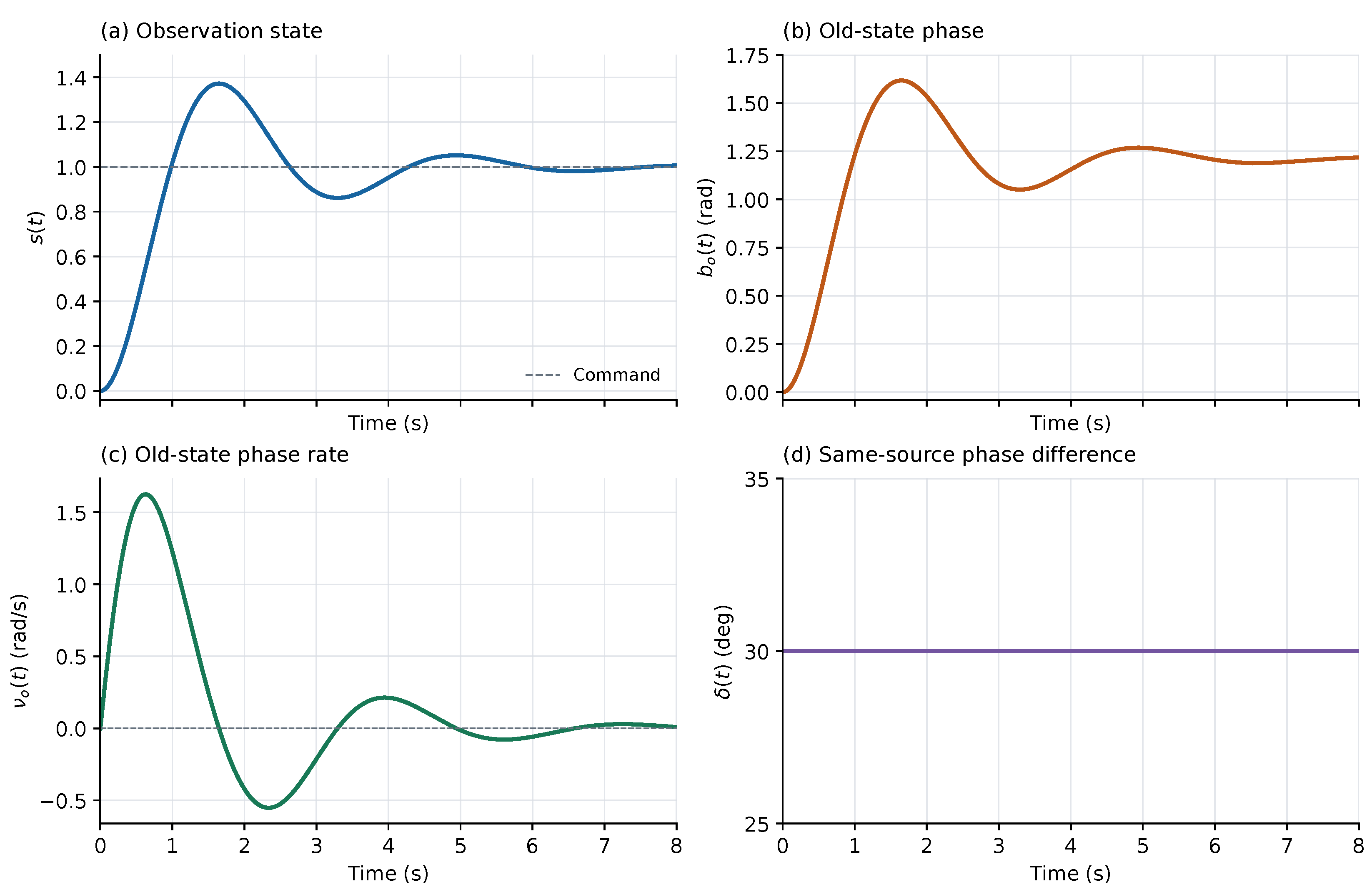
The accompanying calculations check the analytical state equation, convergence of phase-rate finite differences, and reference recovery. Prediction is possible because the actuator equation and complete initial data are known, not because the relative phase is constant.
11.2. Measurement and Feedback Timing
A window may span several configuration intervals. The complete state is propagated in chronological order, and each sample uses the reference and phase correction associated with its actual configuration. At a switch, the configuration identity and reference are updated before accumulation continues. A completed window is stored with its measurement epoch, oscillator history, and complex statistic. The feedback innovation is formed from a prediction of that same window.
A reference change may be represented in the front-end data or in the NCO, provided the remaining phase states use the same convention. Applying it in both places counts the same transformation twice. Because quantization and a general complex rotation do not commute, phase estimation and correction at different bit depths require an explicit observation-error model.
A delayed observation belongs to the window it actually covers. Updating the current state requires propagation from the measurement epoch to the update time. Interpolation or smoothing that uses future samples incurs a buffering delay. Preserving these time relations keeps the hybrid state equations consistent with the actual readout.
12. Joint Tests of Background Dependence and Perturbation Scaling
The two-mode dynamics predict both a background-dependent oscillation frequency and a definite nonlinear phase waveform. They can be tested together by calibrating the device and readout on one data set, then predicting trajectories prepared at other backgrounds and amplitudes. The following protocol is conditional on a physical realization of the planar conservative action. Numerical values specify a dimensionless design, not instrument performance.
12.1. Device Characterization and Free Evolution
An experimental control setting is not automatically a parent-field component. For a recorded device state , the following map must be established in a common reference convention:
The map must be established by independent state measurements, a derivation of the device action, or calibration, with an uncertainty assigned to each quantity. In particular, cannot be inferred trial by trial from the frequency being tested. No physical realization of Eq. (153) is established in this paper; all proposed tests are conditional on it.
Each trial prepares a background, applies an initial perturbation, and releases the system. The values refer to the parallel components before release. Afterwards, those components evolve under the original equations and must not be clamped by a controller. The nominal initial data are
These data satisfy the zero Gauss condition. Nonzero initial velocities, residual forcing, out-of-plane components, and reference drift must be bounded by independent records and propagated into the prediction. All trials use the same fixed analyzer and coherent reference. Uncertainties in admissible initial states are parametrized on the Gauss constraint surface. A measured violation of that constraint is a preparation or model discrepancy, not an additional fit variable. Any auxiliary characterization that disturbs the free evolution must also be included in the model.
The required characterization concerns the action as well as the readout. A programmed simulator can reproduce these equations and assess the measurement procedure, but this alone does not identify the dynamics of an unprogrammed physical system.
12.2. Squared-Frequency Differences Across Backgrounds
For a nonzero background and small perturbations, Eq. (81) gives
Taking as a calibration background yields
The common intercept cancels, but the units and scale of the background components still require independent calibration. If phase data are needed to estimate , only a prespecified calibration set may be used; the parameter is then held fixed throughout the tests. The frequency relation identifies the time scale set by , not f and separately.
For the frequency diagnostic, eliminate the linear constant, sine, and cosine coefficients at each candidate frequency, then minimize the resulting residual over a fixed band and time interval. This is a separable nonlinear least-squares problem [16]. The small-amplitude expansion below concerns the noiseless, amplitude-normalized waveform: assume that its limiting profile has a unique interior frequency minimum at , with nonzero second derivative, and that the normalized waveform depends smoothly and evenly on . For the translation-invariant windows used below, integration changes the linear sinusoidal coefficients but preserves this frequency. More general window operators must also be applied to the fitting template. The implicit function theorem then gives
The combination in Eq. (157) cancels the leading finite-amplitude shift of this fixed diagnostic. It does not assert a unique frequency for an arbitrary nonlinear trajectory. With fixed measurement noise, the limit is also a loss-of-signal limit; the regular noiseless expansion supplies a bias model, not a guarantee of statistical precision. The primary comparison remains the full phase trajectory passed through the calibrated readout operator.
12.3. An Independent Prediction of the Cubic Phase Coefficient
The dynamics specify more than a scaling exponent. For the initial data (154), a perturbation expansion determines the coefficient, sign, and time dependence of the cubic phase term:
Here , , and . Set . The second-order terms in the parallel equations give
Both coefficients and their first derivatives vanish at . With , the angular equation and Gauss constraint reduce the third-order calculation to
Proof.
Substitution of Eq. (158) into the moving-frame equations gives and . Integrating twice gives Eq. (159). Let denote the transverse cubic coefficients. The angular equation yields , while the cubic Gauss condition gives
Differentiating the angular equation once and combining it with this relation eliminates and gives Eq. (161). □
The solution can also be written by quadrature:
12.4. Signed Pairs and Cancellation of the Linear Term
For each amplitude, prepare both positive and negative perturbations and define the phase increment relative to the common pre-release reference. Form
Reflection symmetry gives in the ideal model. Signed pairing also cancels common errors that are even in the perturbation sign; independent drift and odd instrumental nonlinearities remain. The second subtraction removes the linear term exactly:
For a fixed linear functional with , Eq. (164) implies . The weights are selected from the predicted waveform or an independent calibration record before the test data are analyzed. The full contrast, rather than its potentially unstable ratio, is the primary observable.
The ratio becomes unstable when its denominator approaches the noise level. Primary tests should compare the full prediction for , or its prespecified projection. The factor-of-eight ratio is a secondary check when the signal-to-noise ratio is adequate. Finite-amplitude comparisons must retain the higher-order remainder in Eq. (164).
12.5. Cubic Terms Generated by the Integration Window
Let be a fixed, amplitude-independent, nonnegative normalized kernel with compact support. Suppose the phase has a uniform odd expansion in on that support, as it does for the prepared planar family. After reference calibration, the constant-amplitude readout gives
Since , the logarithm has a unique continuous branch near with value zero there. Expanding on that branch yields
Angle brackets denote averages with the same kernel. The cubic contribution is obtained from : the first cumulant contributes , and the third cumulant contributes the negative central-moment term.
Even when the physical phase is strictly linear in amplitude, so that , the window can generate a cubic readout term. The experimental prediction must therefore replace by in Eq. (164), or apply the actual window operator directly to the full complex response before forming the same contrasts. Cubic scaling alone cannot distinguish parent dynamics from integration effects. Varying the window width provides a readout control: the physical trajectory is unchanged, while the window contribution changes according to the calibrated operator.
13. Independent Calibration, Blinded Trials, and Uncertainty
13.1. Calibration and Allocation of Trials
Physical calibration covers the formation map, timestamps, phase sign, analyzer, readout transfer function, and preparation errors for each initial state. Any phase record used to estimate the common coupling belongs exclusively to the calibration set. Without independent support for the formation map, the same frequency data cannot identify both the background scale and the parent coupling.
After calibration, the parameters, data windows, exclusion rules, trial sequence, and analysis procedure are fixed in a single protocol record. During blinded testing, validity is assessed only through prespecified quality criteria, not through agreement with the predicted phase. Blanks, reference playback, and repeated background checks are interleaved in randomized trial blocks. One complete trajectory is one repeat; overlapping correlation windows are not independent samples.
Table 1 gives a reproducible dimensionless design. Since the parent time scale has not been calibrated on a physical device, the listed frequencies are not in hertz. Frequency trials use for zero-amplitude extrapolation. Scaling trials use on the background . The larger amplitude serves only to examine finite-amplitude corrections during protocol development. Repeat counts follow from the independent noise assessment below.
ROT and CAL have the same linear phase frequency. For the same initial perturbation, however, their linear phase amplitudes have ratio . NULL belongs to the exact constant-phase family: its internal state may evolve while the prescribed phase remains fixed. No nonzero oscillation frequency can be read from that phase channel, so the internal restoring frequency must not be entered as a measured phase frequency.
The frequency diagnostic uses the fixed interval ; the scaling test uses . The coherent-window width is , and readouts are evaluated only where complete windows are available. Sampling and window rules are the same for every group. A physical implementation must convert these settings using the calibrated and fix the bandwidth, duration, and trigger treatment before analysis.
13.2. Propagation Through the Readout Model
The residual in the squared-frequency difference is
The common calibration group, field-amplitude scale, and clock correlate the residuals. Let collect the calibrated inputs and let be the derivative of the residual vector with respect to them. If the calibration errors and subsequent repeat errors are independent, first-order uncertainty propagation gives
Otherwise their cross-covariances must be retained. This is the multivariate law of uncertainty propagation [17]. Finite-amplitude extrapolation and independently bounded systematic discrepancies are carried separately from the random covariance.
Initial velocity, release-time error, damping, and out-of-plane motion also change the waveform. For the fixed dynamics and readout operator, sensitivities can be propagated along the nominal trajectory:
The sensitivity equations propagate independently characterized deviations into the same measured statistic. A damping contribution larger than the prespecified conservative-model tolerance calls for a different dynamical model and a new test, rather than a post hoc adjustment of the frozen prediction.
Perturbation amplitudes must use their calibrated values. If neighboring amplitudes are not exactly in a two-to-one ratio, the contrast has cubic coefficient . Continuing to subtract with the nominal factor 2 leaks the linear phase into the cubic observable. When the amplitude error is of order , its relative contribution to the cubic signal grows as . Smaller perturbations do not necessarily make the test more accurate.
13.3. Correlations, Repeats, and Detectable Signals
Suppose the phase score obtained by applying the fixed functional to one complete trajectory has independent random error with standard deviation . With n independent repeats for each sign and amplitude, half the difference of the signed means has variance . Hence
The covariance arises because the half-amplitude data are reused in neighboring contrasts. Likewise,
If drift correlates trials, the actual block covariance must replace these independent-error expressions.
If a signal must exceed q random standard deviations to be considered detectable, then, while the cubic term dominates,
Thus halving the perturbation requires approximately 64 times as many independent repeats when noise and weights are unchanged. This is a detectability condition, not a significance test of the entire model. Odd instrumental nonlinearities and systematic calibration errors do not vanish with additional repeats.
For illustration, normalize , assume a single-trial score standard deviation of rad, and take . At , the ideal cubic contrast signals are rad, respectively. The bound requires at least repeats per sign. These hypothetical values illustrate the budget; they are not specifications of an instrument. Actual repeat counts must also support variance estimation and the block design.
13.4. Prespecified Decisions and Controls
Collect the prespecified measured features in s and the frozen model predictions in m. Assume that , where , is known and positive definite, and the fixed nonempty compact set contains the systematic bias . Define
and reject at , with . Under the stated null model,
so the rejection probability is at most . The bound relies on the independently fixed bias set and known covariance. An estimated covariance, nonlinear calibration uncertainty, or non-Gaussian error distribution requires a threshold calibrated for that procedure; the displayed chi-square quantile then has no automatic exact finite-sample interpretation.
Two controls serve different purposes. A readout control passes a known reference phase through the same window and electronics to measure instrumental cubic terms; it does not test parent dynamics. A dynamical comparison retains the same linear frequency and initial response but allows only the linear physical phase, followed by the same window operator. It therefore contains the window-generated cubic term in Eq. (166), but not . The difference between this comparison and the full prediction isolates the nonlinear dynamical contribution considered here.
A reproducible discrepancy outside this uncertainty model would reject the specified conservative dynamics together with the proposed device map. An absent map or undetectable signal leaves the test inconclusive. Agreement would support that realization over the tested initial states, but would not by itself establish uniqueness among all physical models.
14. Discussion and Conclusions
The distinction between transport and prediction can be made precise without assigning independent dynamics to a measured phase. A complex response supplies its phase differential, while the state equations determine the path on which that differential is evaluated. In the projector–connection model studied here, the parent action provides those state equations and their constraints. The homogeneous two-mode sector is an exact reduction with a global classical flow. Horizontal transport and a fixed analyzer then define the coherent observable.
The main realization result concerns the invariant planar sector. Its phase increments depend on seven inner products that evolve autonomously. The exact nonzero determinant of the phase-derivative map gives a matching local lower bound, so seven states are necessary as well as sufficient near generic regular initial data. This is a dimension statement about the chosen passive protocol, not about the observation axis in every physical system. The initial phase remains a separate reference, and the Gram chart may require replacement along a trajectory.
The exceptional sets reveal why an instantaneous readout is not a substitute for a dynamical state. Near equilibrium, only one linear oscillatory mode reaches the phase, yielding a two-state predictor. On the constant-phase family, the internal fields evolve while every phase increment vanishes. Away from those sets, higher-order couplings make additional state directions visible. The phase-behavior quotient provides a common language for all three cases while retaining their different admissible initial-data ranges.
A related distinction appears in array processing. Relative alignment converts a response to the current reference; predicting or restoring a fixed reference also requires the reference’s own evolution. Coherent integration introduces a further dependence on the trajectory within the measurement window. The finite-window formulas identify amplitude-weighted phase biases and cancellation that cannot be corrected by a single rotation after accumulation.
The background-frequency relation and cubic phase waveform supply conditional experimental predictions of the parent model. Signed perturbations and amplitude contrasts suppress the linear term, but the window contributes its own cubic phase. Comparing the complete complex readout separates these effects. The resulting protocol makes clear what must be calibrated independently and which data remain available for prediction tests. All numerical results reported here are model calculations. A physical test requires a device whose action and readout admit the stated reduction, followed by uncertainty-controlled comparison on initial states excluded from calibration. Such a test would assess this dynamical realization, rather than the scalar phase identity alone.
Data Availability Statement
The accompanying source archive contains the numerical programs, exact rational derivative matrices, synthetic trajectories, figure-generation scripts, and the proposed experimental record templates. No experimental data are reported. Computational methods and numerical settings are given in the appendices.
Appendix A. Homogeneous and Planar Numerical Solutions
Appendix A.1. Homogeneous Trajectories
The homogeneous equations, horizontal lift, and scalar phase equation were integrated with the explicit DOP853 method [18]. The initial data are those of Eqs. (41) and (55). Two tolerance levels were used, with no renormalization or projection onto the constraint surface during integration.
The interval contains 4001 output points. Baseline relative and absolute tolerances are , tightened to . The initial energy is . Dense sampling and local minimization give a minimum readout modulus of at . This is a numerical minimum, not a rigorous analytic lower bound.
At the tighter tolerances, the continuous phase increases from 0 to rad, and the maximum dimensionless phase rate is . The table reports maximum residuals on the common output grid. Energy errors are relative; all other entries use the indicated absolute norms. Phase derivatives are taken with respect to dimensionless time.
Figure A1.
The homogeneous parent system and its phase readout. The projector direction and connection fields evolve together; phase rate and acceleration are computed from the same trajectory. Initial data are given in Eq. (41), and time is dimensionless.
Figure A1.
The homogeneous parent system and its phase readout. The projector direction and connection fields evolve together; phase rate and acceleration are computed from the same trajectory. Initial data are given in Eq. (41), and time is dimensionless.
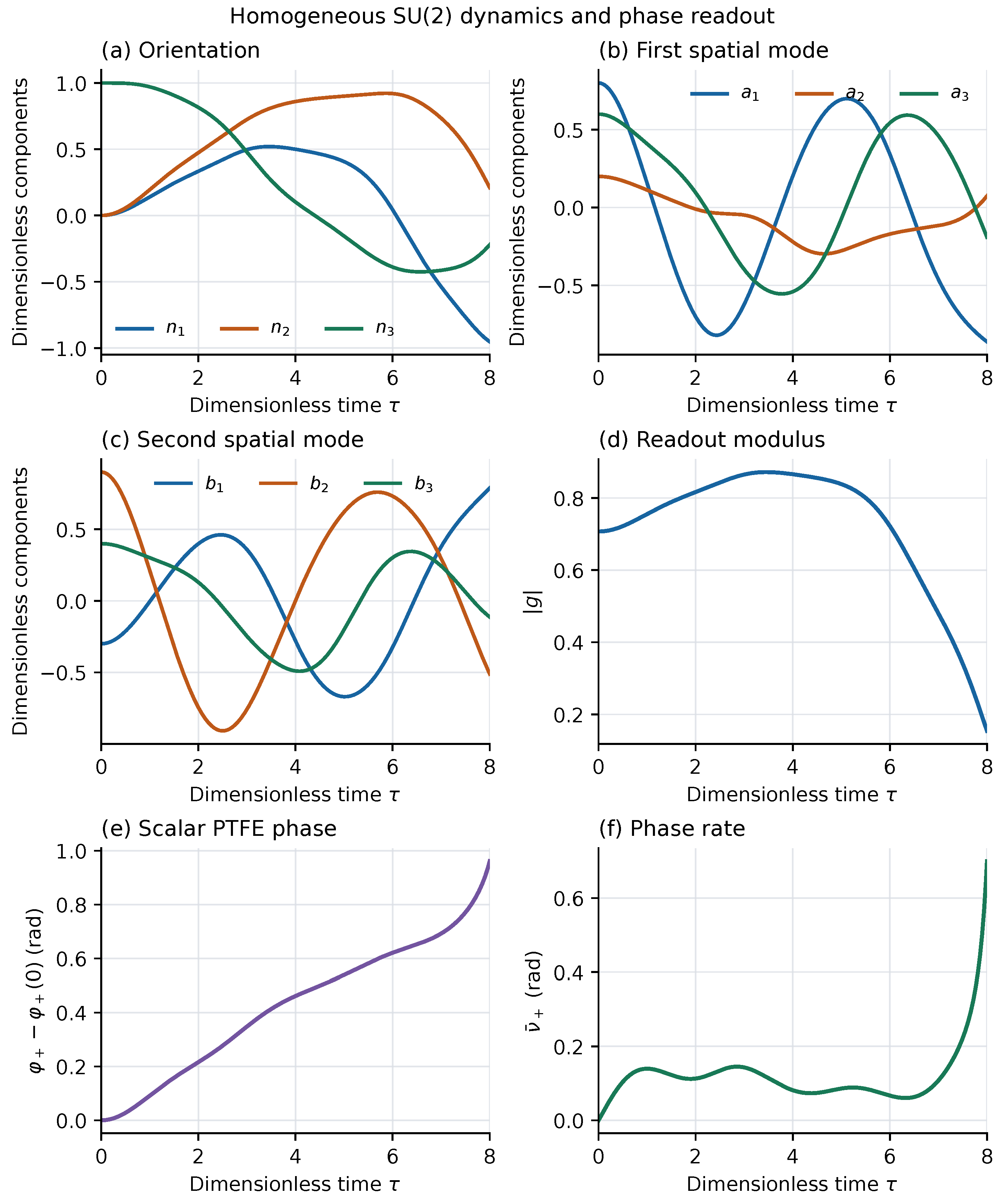
| Quantity | Maximum residual |
| Relative energy error | |
| Gauss constraint | |
| Unit-length error | |
| Tangency constraint | |
| Lift compatibility | |
| Horizontality | |
| Complex difference: integrated scalar phase versus | |
| Phase-rate difference: complex-vector calculation versus Eq. (52) | |
| Phase-acceleration difference: complex-vector calculation versus Eq. (53) | |
| Independent potential directional-derivative error | |
| Phase-rate difference between tolerance levels | |
| Phase-acceleration difference between tolerance levels |
Figure A2.
Energy, constraint, and phase residuals from direct integration. The curves check energy conservation, the projector and Gauss constraints, and compatibility between the horizontal lift and scalar phase transport.
Figure A2.
Energy, constraint, and phase residuals from direct integration. The curves check energy conservation, the projector and Gauss constraints, and compatibility between the horizontal lift and scalar phase transport.
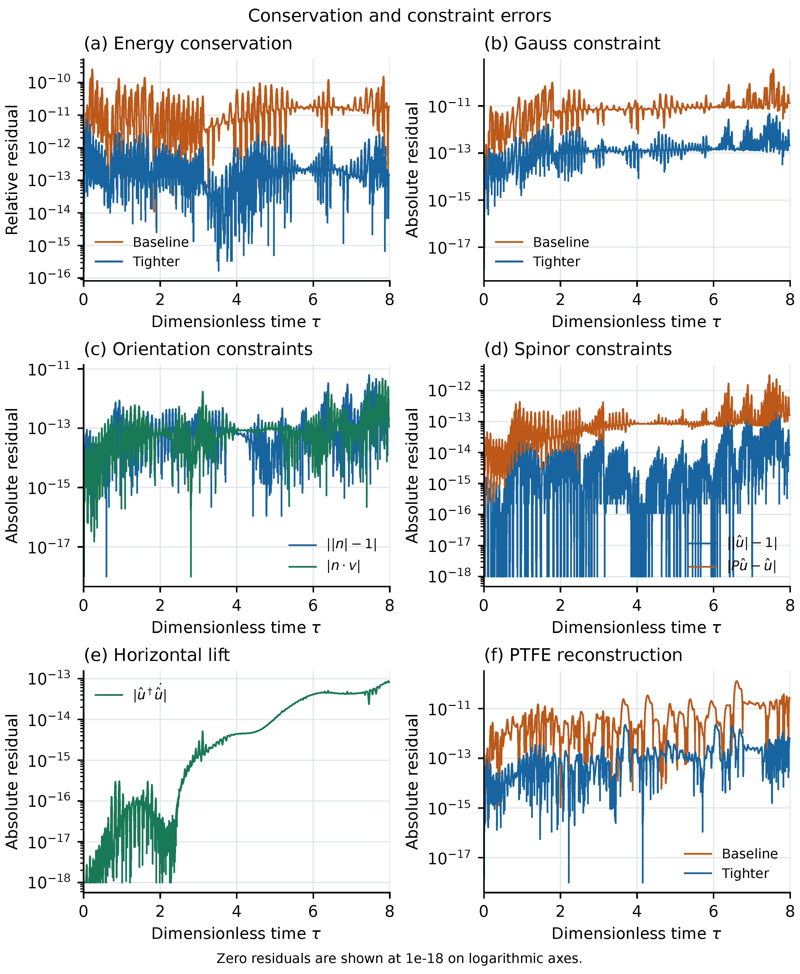
The force calculation was compared with directional finite differences of the potential, restricted to the tangent plane for the projector. The phase rate and acceleration obtained from the complex state were compared with Eqs. (52) and (53). Finally, integration of the scalar phase equation was compared with . The analytic initial values provide a further, time-integration-independent comparison.
All entries describe numerical errors for the specified model trajectory.
Appendix A.2. Planar Trajectories and Perturbation Scaling
The moving-frame system (72) and the vector system (34) were integrated independently, including the coherent lift in the latter. Their solutions were compared through the configuration map (63), velocity map (67), and phase relation (77). Neither solution was projected onto a constraint surface.
Using Eq. (40), take , , and . The prediction is
The frequency was fixed at this value for all four perturbation amplitudes. In the figures, denote . The largest perturbation, , has initial phase acceleration ; the values quantify the approach to the cubic remainder.
The comparison window is fixed at three linear periods, , with 4001 common output times. DOP853 relative and absolute tolerances are , tightened to . The resulting phase and phase-acceleration differences between tolerance levels are at most and . A centered finite-difference Jacobian of the vector field at equilibrium independently gives two positive eigenfrequencies of , consistent with . The table uses the tighter integration.
| Quantity | Result |
| Initial phase acceleration | (analytic and numerical) |
| Maximum component difference between coordinate and vector states | |
| Relative energy error (coordinate/vector) | / |
| Coordinate Gauss momentum | |
| Vector Gauss-constraint norm | |
| Absolute difference between phase-rate calculations | |
| Absolute difference between phase-acceleration calculations |
| Maximum phase error (rad) | Error ratio | Numerical order | |
| — | — |
The error ratio divides each row’s maximum error by that in the next row; the numerical order is its base-two logarithm. The results agree with the cubic remainder on a fixed interval. For , nonlinear departures are already visible in the third period: the maximum phase error is about rad and the maximum phase-acceleration difference about . Figure A3 compares the nonlinear trajectory with the predetermined linear prediction.
Figure A3.
Nonlinear phase evolution and the small-oscillation solution at the theoretical frequency . Reducing the initial perturbation decreases their difference on the fixed interval according to Eq. (85). Time and connection components are dimensionless.
Figure A3.
Nonlinear phase evolution and the small-oscillation solution at the theoretical frequency . Reducing the initial perturbation decreases their difference on the fixed interval according to Eq. (85). Time and connection components are dimensionless.
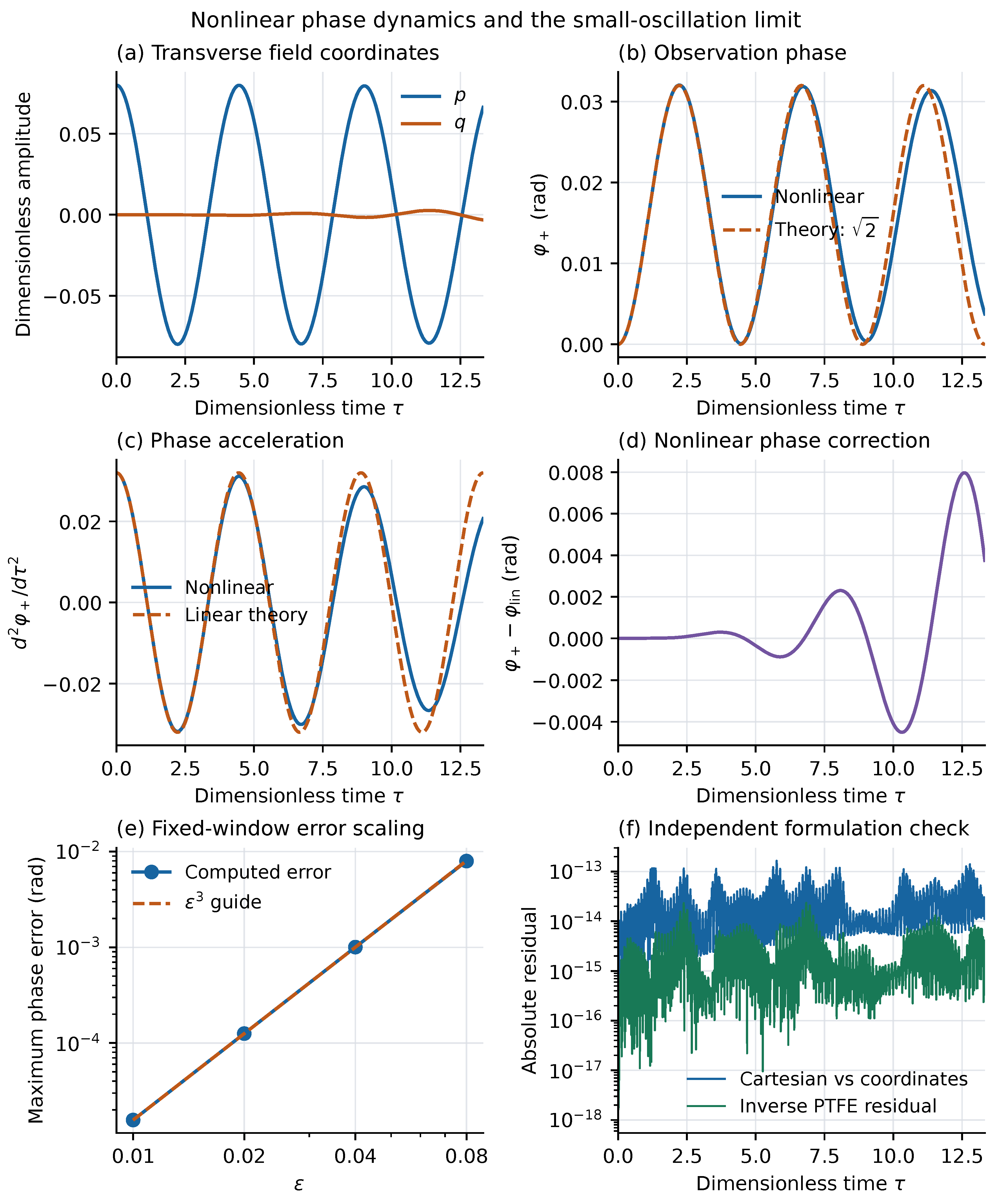
For the constant-phase family, take , , zero initial velocities, and the same background . The two-variable equations, moving-frame equations, and vector equations are solved independently. On the same interval, r decreases to about , while h ranges approximately over . The maximum changes in the two connection vectors relative to their initial values are about and . Yet the vector solution has a maximum phase change of only rad and a phase-acceleration residual of . Maximum component differences between the two-variable solution and the moving-frame and vector solutions are and , respectively, consistent with exact phase constancy.
Figure A4.
Internal motion in the constant-phase family. The connection components in Eq. (87) change with time, while the response projector and coherent readout remain fixed.
Figure A4.
Internal motion in the constant-phase family. The connection components in Eq. (87) change with time, while the response projector and coherent readout remain fixed.
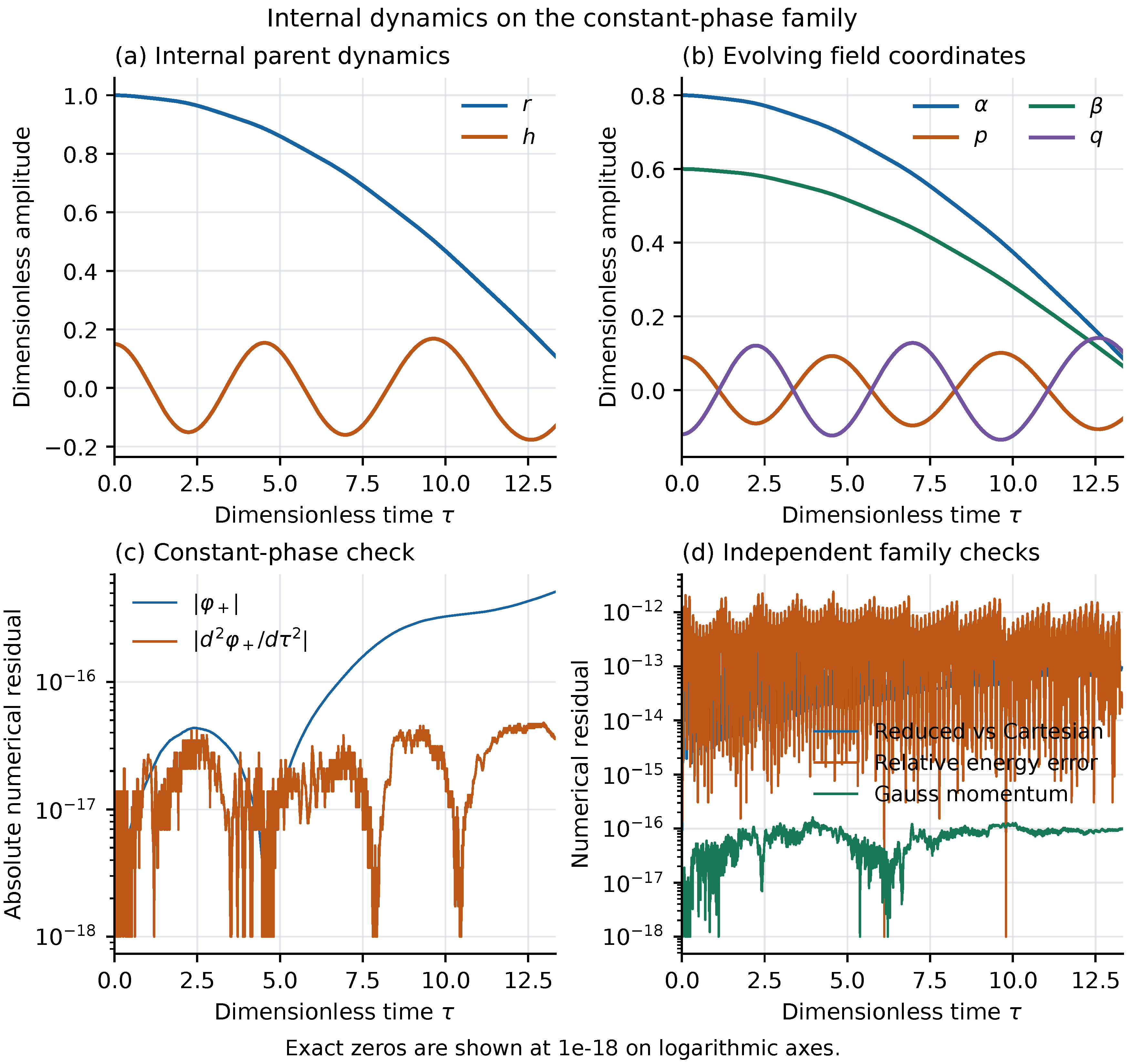
Observable oscillations and internal constant-phase motion arise from the same action but require different information for phase prediction. This motivates a reduced state defined by future phase histories themselves.
Appendix B. Linear Observable Modes and Constant-Phase Trajectories
Appendix B.1. Two States for the Linear Phase Mode
The linear observable mode of Section 6.5 satisfies
Hence
is a closed second-order state and provides local coordinates for the nontrivial observable sector of the linear phase-behavior quotient. To see why the phase rate alone is insufficient, take and . Then
The two states have the same present phase rate but different futures. Adding makes the future unique in the linear model. Including the phase reference gives
This is equivalent to : two variables describe the observable oscillation, and one records the phase reference.
Figure A5 uses , , and . Equation (A4) gives a maximum phase-rate difference of and a maximum phase-increment difference of rad over three periods.
Figure A5.
Two trajectories with the same initial phase rate and opposite phase accelerations: , , and frequency . Their phase increments differ by at most rad.
Figure A5.
Two trajectories with the same initial phase rate and opposite phase accelerations: , , and frequency . Their phase increments differ by at most rad.
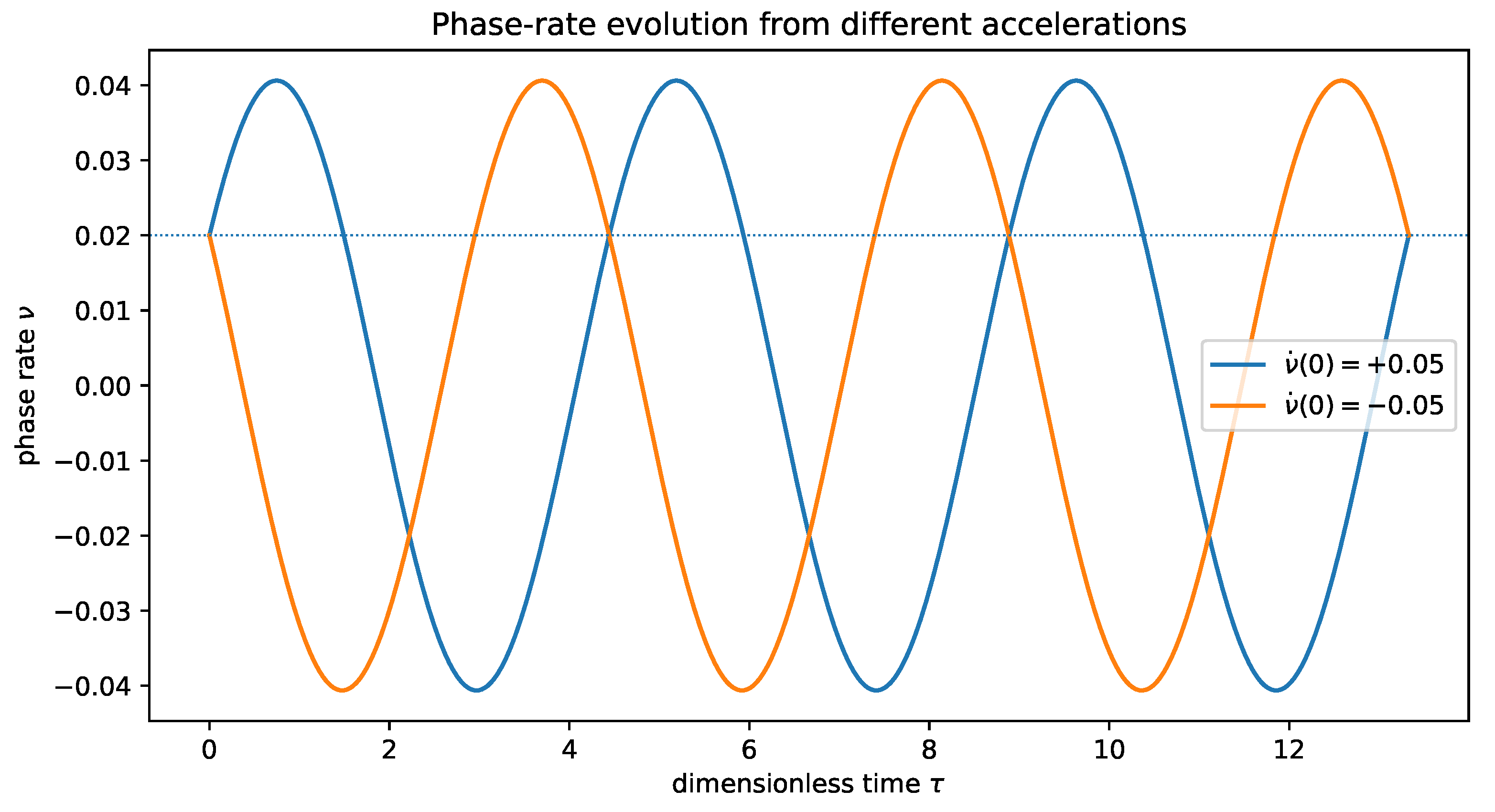
This two-state realization is exact for the linear model, not for the full nonlinear parent system. Equation (85) gives the nonlinear remainder, through which additional parent states can affect future phase. The dimension of the exact behavior quotient must be calculated from the nonlinear equations.
Appendix B.2. A Constant-Phase Behavior Class Under Passive Observation
The exact internal family (87) satisfies
while the internal gauge invariant
may vary with time. With a fixed analyzer and no active intervention, the family produces the same phase increments and belongs to one behavior class. Predicting phase for this restricted family does not require retaining h.
Figure A6 uses the parent solution from Appendix A.2. Starting at , the internal invariant ranges approximately over on the computation interval. The absolute phase residual remains below rad.
Figure A6.
An internal gauge invariant along a constant-phase trajectory. The invariant changes substantially while the phase increment remains zero. Under the fixed passive protocol, these states have the same phase behavior.
Figure A6.
An internal gauge invariant along a constant-phase trajectory. The invariant changes substantially while the phase increment remains zero. Under the fixed passive protocol, these states have the same phase behavior.
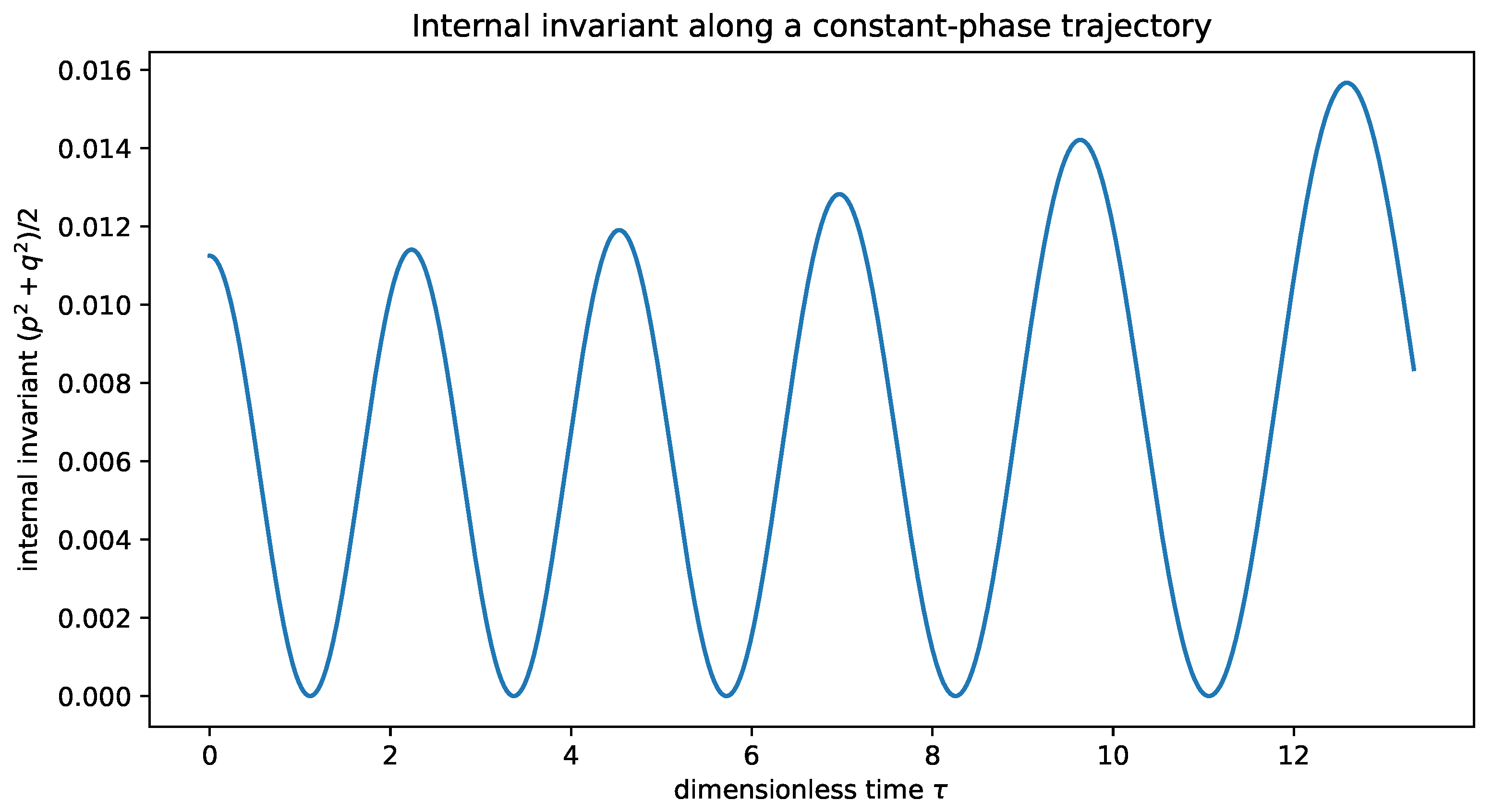
Identical phase behavior means only that the current protocol cannot distinguish the states. It does not identify the complete physical states. Their future behavior must be compared anew when the measurement or control set is enlarged.
Appendix B.3. Reproducing the Analytic Behavior
The script minimal_state_reduction.py recomputes the oscillation example and reads the constant-phase trajectory of Appendix A.2. It checks the analytic phase-rate and phase-increment differences in the first example and phase constancy during internal motion in the second. A separate auxiliary-variable example illustrates redundancy by adding a variable fully decoupled from the output. That example is not used in the parent-dynamics proof or the seven-dimensional rank calculation.
The examples show both why present phase information can be insufficient and why complete internal states can be redundant. Future behavior is the criterion for exact reduction.
Appendix C. Exact Derivatives and Reduced-State Trajectories
Appendix C.1. Exact Differentiation in Two Coordinate Systems
The matrix in Eq. (116) was evaluated with rational Taylor coefficients and differentiated with respect to the initial state. A separate calculation used the eight-component polynomial field (106). If is the inner-product map and x the eight-component coordinate vector, the two results satisfy
In the order , the remaining one-dimensional kernel is generated by
which is the tangent to the common rotation at this point. Adding successive phase-derivative rows gives exact ranks .
Symbolic chain-rule calculations also verify all seven projected equations, , and energy conservation, with exact zero residuals. The derivative map has rank three at and rank two at the eight-variable equilibrium , in agreement with the analytic classification.
Appendix C.2. Independent Integration of the Reduced and Parent Systems
Use the initial state (114) on the fixed dimensionless interval , with 2001 common output points. The corresponding initial configuration and velocity in the five-coordinate system are
The Gauss momentum is zero and the normalized energy is 11. The moving-frame system and seven-inner-product flow are integrated separately, and their inner products and accumulated phases are compared afterward. Neither trajectory is renormalized, corrected to satisfy constraints, or regularized by clipping a singular denominator.
Results for two DOP853 tolerance levels follow. Maxima are taken on the common output grid, and relative energy errors are normalized by the initial energy.
| Quantity | Baseline | Tighter tolerances |
| Relative/absolute tolerance | ||
| Maximum inner-product component difference | ||
| Maximum accumulated-phase difference (rad) | ||
| Maximum phase-rate difference | ||
| Maximum parent-coordinate Gauss residual | ||
| Maximum relative energy drift in seven-state flow |
The tighter integration gives final phase rad and a smallest sampled Gram determinant of . These values refer to the specified finite interval. If a subsequent trajectory crosses the boundary of this chart, the original parent equations remain available.
Appendix C.3. State Prediction and Estimation from Measurements
These trajectories illustrate the seven-state realization away from equilibrium. The two-state approximation is instead appropriate to the small-perturbation regime quantified in Appendix A.2.
Local observability is not a noise-conditioning estimate. A practical observer would propagate the state equations and assimilate coherent-window measurements, rather than estimate seven phase derivatives by differencing. Its initialization and error growth require a separate analysis [10]. The ASMO application below has its own formation map and therefore its own minimal-state problem.
Appendix D. Numerical Evaluation of the Proposed Tests
The proposed analysis was evaluated on synthetic trajectories from the full moving-frame equations. Coherent integration, signed pairing, half-amplitude contrasts, and fixed projections were applied to these trajectories, while was obtained independently from Eq. (161). The calculation uses the parameters and windows specified in Section 13.
For the nominal background , use windows of width and weights chosen in advance from , normalized so that . The ratios of neighboring contrasts are
Finite-amplitude corrections prevent the ratios from being exactly eight; reducing the perturbation brings them toward the cubic prediction. At short times, the independent equation gives
The difference is consistent with the higher-order terms in the short-time expansion.
Figure A7.
Cubic phase waveform recovered from windowed signed contrasts. Division by gives the independently calculated cubic coefficient in the small-amplitude limit. The time window and projection weights are the same for every trajectory.
Figure A7.
Cubic phase waveform recovered from windowed signed contrasts. Division by gives the independently calculated cubic coefficient in the small-amplitude limit. The time window and projection weights are the same for every trajectory.
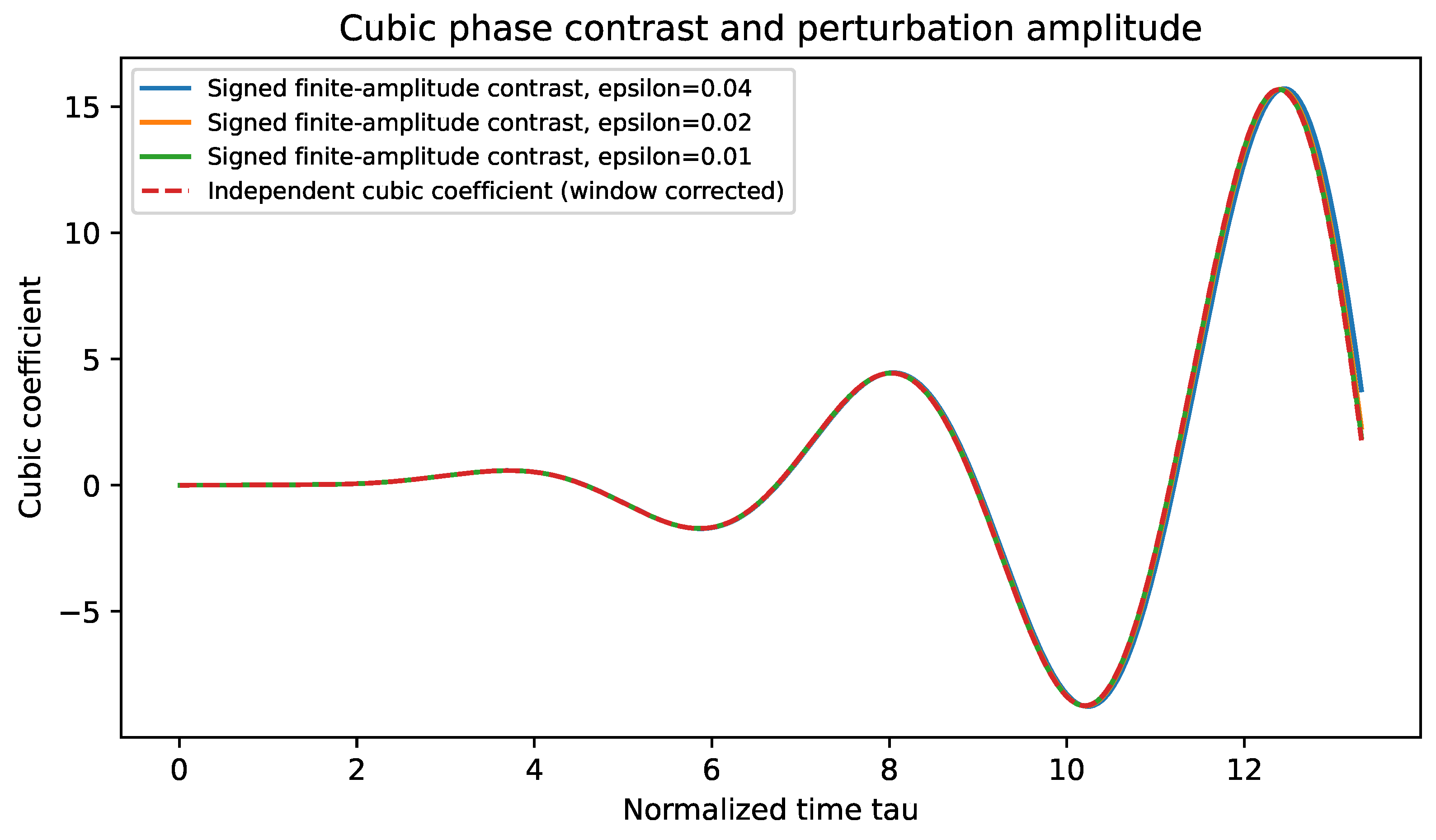
The six nonzero-signal backgrounds use the same frequency diagnostic and time window. The largest difference between the two-amplitude extrapolation and the theoretical is . This checks the numerical procedure, not the frequency accuracy of a physical device. The NULL group has identically zero model phase.
Figure A8.
Background dependence of the squared phase frequency. The line is the small-oscillation prediction; the markers are estimates from synthetic parent trajectories, using the same frequency diagnostic and amplitude extrapolation at each background.
Figure A8.
Background dependence of the squared phase frequency. The line is the small-oscillation prediction; the markers are estimates from synthetic parent trajectories, using the same frequency diagnostic and amplitude extrapolation at each background.
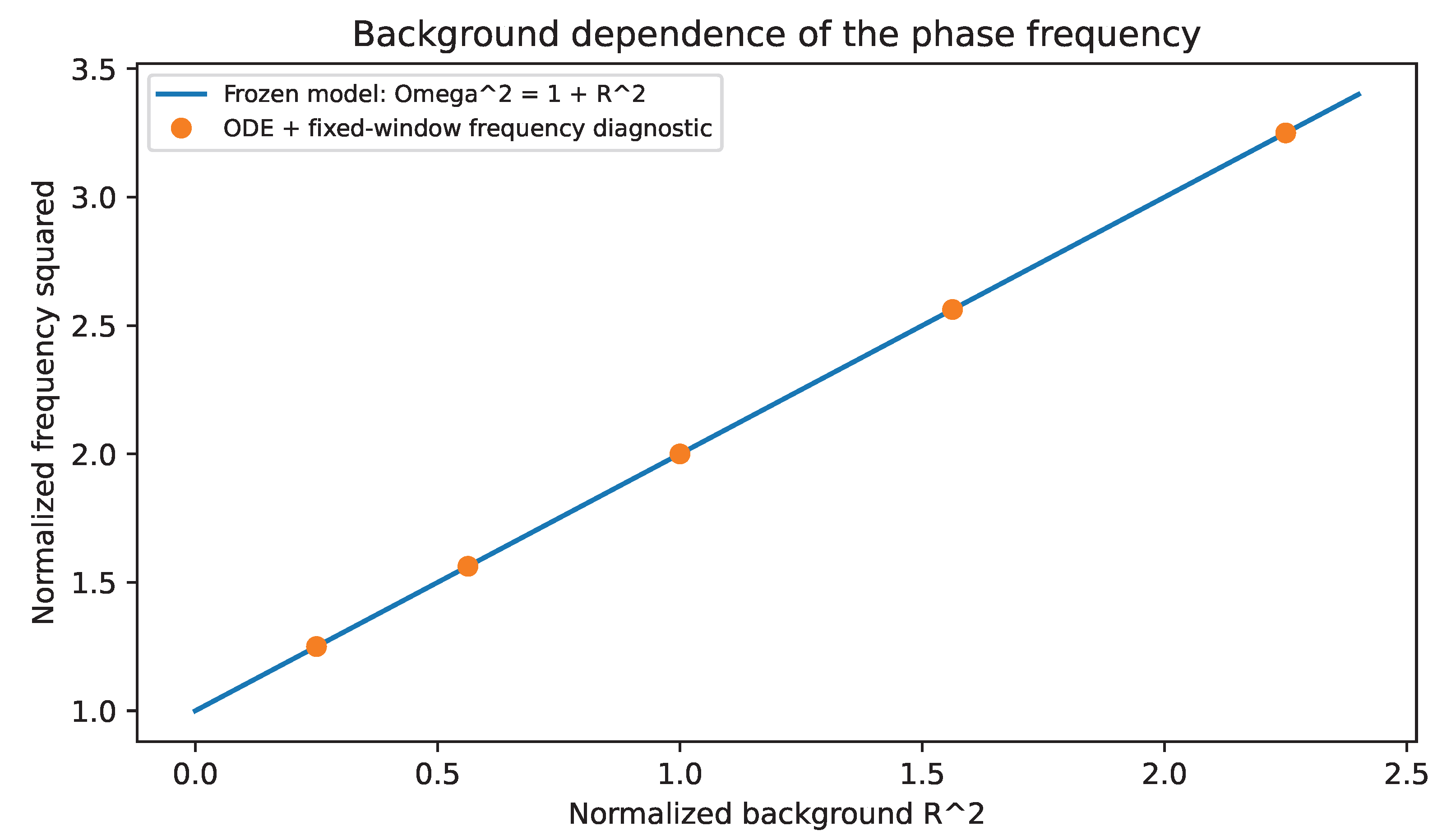
A separate window of width , centered at , checks the cubic readout correction. The independent prediction is , compared with from finite-amplitude differences, an absolute discrepancy of . The window-generated correction itself is . This wider window makes the contribution numerically visible without changing the main protocol’s window width.
The synthetic examples separate the dynamical cubic waveform from the window contribution and verify that the prescribed statistics recover both. They provide a reproducible analysis procedure for a future physical realization.
Appendix E. Independent Phase Loads and Curvature Forces
The horizontal phase above is a readout of the parent state, not an independent degree of freedom acting back on it. If a physical system contains a phase variable with its own conjugate load, transport can instead enter the path dynamics through an action. This section treats that distinct case.
Appendix E.1. Variation of the Transport Constraint
Let be the real comparison connection for the observation branch, and let be the joint system’s path Lagrangian. The scalar-response branch uses ; a multicomponent response or independent parent connection requires its own specified comparison geometry. Introduce
Here is the local transported phase and J its conjugate variable. For dimensionless phase, J has units of action, and its initial value is fixed by physical preparation of the load.
The transformation , leaves the transport term invariant. Define
Variation with respect to gives, respectively,
Appendix F provides the variation in detail. The path and transport equations share one action; the inertia and interactions in are supplied by the physical system.
Appendix E.2. Inertia, Dissipation, and External Driving
Consider a mechanical path Lagrangian and a quadratic dissipation function,
where the inertia metric H is positive definite, C is symmetric positive semidefinite, and is the Rayleigh dissipation function. Write the external force as and the Christoffel symbols of the first kind as
The Lagrange–d’Alembert equations and PTFE then form
Given and initial data , Eq. (A17) defines an initial-value problem. Smooth coefficients and invertible inertia ensure local uniqueness. The solution continues for as long as it remains in a compact subset of the regular domain on each finite interval.
The response determines , whereas inertia, potential, and dissipation come from the system action, a device model, or identification data. The dual-axis structure permits joint dependence on but does not fix these quantities numerically.
Appendix E.3. Canonical Momenta and Energy Balance
Without dissipation or external driving, the velocity-linear phase term produces the constraints and . Their Poisson bracket is nonzero, so they form a second-class pair. Eliminating them leaves as conjugate variables, after which the configuration velocities admit the usual Legendre transform [14]. The momenta are
The Hamiltonian is
Hamilton’s equation recovers the transport law. The connection term in the configuration momentum records the coupling between phase load and path.
For the mechanical energy , and with no explicit time dependence in , Eq. (A17) gives
This follows by contracting the equations of motion with velocity. The curvature force does no total mechanical work because . External driving supplies energy, and dissipation removes it. Explicit time dependence of the inertia, potential, or connection adds the corresponding energy-exchange terms.
Appendix E.4. Curvature Forces on the Two Axes
Mixed curvature enters both equations of motion. With the sign convention of Eq. (A21), its powers along the two velocity subspaces are
The powers cancel, describing exchange between the two types of motion. If has mixed kinetic terms or a nonseparable potential, this remains a force–velocity identity, not a unique decomposition into two energies.
Appendix E.5. Observation Motion at Fixed Physical State
If an experiment holds , restrict the action to that section. With and , the equations are
All coefficients are evaluated at , and denotes the first-kind Christoffel symbols of the restricted inertia metric. Holding the physical state fixed generally requires reaction forces. Ideal reactions do no work because . Equation (A25) describes this constrained experiment, not arbitrary free joint motion.
For the original scalar PTFE, , so Eq. (A25) reduces to
The first equation determines the observation state, and the second maps that motion into phase. Substituting the state acceleration into Eq. (12) gives
Appendix E.6. The Flat Connection of a Scalar Response
For a nonzero scalar response,
Because is globally defined, its winding along a closed path is an integer and the exponential holonomy is unity. The one-form need not be globally exact as a real-valued form: nonzero integer periods are possible. This distinguishes the scalar response connection from a general flat connection, whose holonomy need not be trivial [6].
Locally, , and the transport term is . The change of coordinates gives
The phase variables then decouple locally from the base path: , while the path obeys the equations of . Since J is itself varied, is not generally a total derivative that can simply be discarded. The coordinate transformation establishes the decoupling.
Mixed sensitivity may be nonzero even when curvature vanishes. For example,
The phase satisfies and . The crossed term reflects joint dependence on the two axes, whereas curvature takes an antisymmetric derivative. They represent different structures.
Appendix E.7. Comparison Geometry of Multicomponent Responses
For a multicomponent response , set . The comparison connection and curvature are
For the curvature vanishes. For , motion of the projective direction may give nonzero curvature, as in the geometric-phase construction [5,6,7]. Its horizontal factor is in the sign convention used here. This multicomponent connection is distinct from after the response has been combined into a single scalar. An independent parent connection additionally requires its own equations of motion.
Horizontal transport in a curved connection generally depends on the path, not only its endpoints. It differs from the phase differential of an everywhere nonzero single-valued scalar , which necessarily satisfies Eq. (A28). A multicomponent comparison geometry must therefore specify how path transport enters the actual coherent readout.
Appendix E.8. An Integrable Test Model with Mixed Curvature
Take the two-component response
Direct calculation gives
Choose the test-path kinetic term
Substitution into the common path action yields
Here and J are the test-path inertia and independent phase load. This example checks Eq. (A12); it is not the homogeneous parent-field reduction of Section 4. Time translation and the cyclic coordinate s give the conserved quantities
The regular motion can then be found by quadrature:
The two-axis path and transported phase are determined together, with the effect of mixed curvature explicit in the equations. ASMO’s scalar response instead belongs to the flat branch described above.
Appendix F. Variation of the Path Action with Explicit Time Dependence
Take compactly supported variations of Eq. (A12). Variation of J gives ; variation of , followed by integration by parts, gives . The configuration Euler–Lagrange expression is
If the connection depends explicitly on time, use the extended one-form . The transport term becomes , so that
The Hamiltonian then acquires . For a time-dependent scalar response , take both and . The extended connection is still locally , so as well. Explicit time dependence does not by itself generate curvature of a scalar-response connection.
Appendix G. Local Expansion of Short-Window Bias
Let be a nonnegative normalized kernel supported on and symmetric about . Write and , so that and the fourth moment is . Suppose is four times continuously differentiable near the center, , and the derivatives are bounded in the neighborhood considered. On a common local phase lift, as ,
Subtracting the two expressions gives
If d is constant while the amplitude ratio changes, the leading bias is . This is the local coupling between amplitude weighting and common-phase variation; Eq. (138) gives a discrete example without a short-window approximation.
Appendix H. Exact Phase-Derivative Recursion and Reproducibility
Write , with each coefficient also carrying its derivatives with respect to the seven initial components. For the rational vector field, compute successively
Differentiation with respect to the initial state yields . Series products use finite convolution, and reciprocals follow recursively from the coefficients of a product equal to one. All arithmetic is rational. The seven-dimensional rational equations and eight-dimensional polynomial parent equations are evaluated independently and checked against the chain rule in Eq. (A8).
The main source is PTFEDynamics20261007v9EN.tex. Compile it twice with pdfLaTeX, or use latexmk -pdf, in a standard TeX distribution. The accompanying archive contains the manuscript, figures, data, five theoretical verification scripts, and the proposed experimental-analysis script.
Running python run.py recomputes the exact rank, compares the seven-state and original parent integrations, and runs the proposed experimental-analysis checks. In generatedrank/, certificate.json records the exact matrices, determinant, ranks on the different state sets, and error definitions. The files jetjacobian.csv and rawjetjacobian.csv store derivatives in the two coordinate systems; trajectory.csv stores states and phases on the common output grid. The program stops and reports an error if a coordinate denominator is invalid, integration fails, or an assertion is violated.
The scripts runchecks.py, numericalclosure.py, observationcoordinates.py, and minimalstatereduction.py check the scalar and window examples, vector parent system, moving-frame coordinates and oscillations, and behavioral examples, respectively. They require Python with NumPy, SciPy, SymPy, Matplotlib, and pandas. All reported data are generated from the models and initial conditions stated in the paper.
References
- Meng, X. “A set-theoretic derivation of Physobser axiom irreducibility, minimality, and essential uniqueness of the physical–observation dual-axis structure,”. Prepr. (2026) Version 2. [CrossRef]
- Meng, X. “The phase transport fundamental equation on the physical–observation dual-axis structure,”. Prepr. (2026) Version 2. [CrossRef]
- Pancharatnam, S. Generalized theory of interference, and its applications. Part I. Coherent pencils. Proc. Indian Acad. Sci. A 1956, 44, 247–262. [Google Scholar] [CrossRef]
- Kato, T. On the adiabatic theorem of quantum mechanics. J. Phys. Soc. Jpn. 1950, 5(6), 435–439. [Google Scholar] [CrossRef]
- Berry, M. V. Quantal phase factors accompanying adiabatic changes. Proc. R. Soc. Lond. A 1984, 392(1802), 45–57. [Google Scholar] [CrossRef]
- Simon, B. Holonomy, the quantum adiabatic theorem, and Berry’s phase. Phys. Rev. Lett. 1983, 51, 2167–2170. [Google Scholar] [CrossRef]
- Aharonov, Y.; Anandan, J. Phase change during a cyclic quantum evolution. Phys. Rev. Lett. 1987, 58, 1593–1596. [Google Scholar] [CrossRef] [PubMed]
- Sussmann, H. J. Existence and uniqueness of minimal realizations of nonlinear systems. Math. Syst. Theory 1976, 10, 263–284. [Google Scholar] [CrossRef]
- Hermann, R.; Krener, A. J. Nonlinear controllability and observability. IEEE Trans. Autom. Control 1977, 22(5), 728–740. [Google Scholar] [CrossRef]
- Sontag, E. D. Mathematical Control Theory: Deterministic Finite Dimensional Systems, 2nd ed.; Springer: New York, 1998. [Google Scholar] [CrossRef]
- Lee, J. M. Introduction to Smooth Manifolds . In Graduate Texts in Mathematics, 2nd ed.; Springer: New York, 2012; Vol. 218. [Google Scholar] [CrossRef]
- van der Schaft, A. Equivalence of dynamical systems by bisimulation. IEEE Trans. Autom. Control 2004, 49(12), 2160–2172. [Google Scholar] [CrossRef]
- Yang, C. N.; Mills, R. L. Conservation of isotopic spin and isotopic gauge invariance. Phys. Rev. 1954, 96, 191–195. [Google Scholar] [CrossRef]
- Dirac, P. A. M. Generalized Hamiltonian dynamics. Can. J. Math. 1950, 2, 129–148. [Google Scholar] [CrossRef]
- Marsden, J. E.; Weinstein, A. Reduction of symplectic manifolds with symmetry. Rep. Math. Phys. 1974, 5(1), 121–130. [Google Scholar] [CrossRef]
- Golub, G. H.; Pereyra, V. The differentiation of pseudo-inverses and nonlinear least squares problems whose variables separate. SIAM J. Numer. Anal. 1973, 10(2), 413–432. [Google Scholar] [CrossRef]
- Joint Committee for Guides in Metrology, Evaluation of Measurement Data—Guide to the Expression of Uncertainty in Measurement. In JCGM; BIPM, 2008; Volume 100, p. 2008. [CrossRef]
- Hairer, E.; Nørsett, S. P.; Wanner, G. Solving Ordinary Differential Equations I: Nonstiff Problems, 2nd ed.; Springer: Berlin, 1993. [Google Scholar] [CrossRef]

Table 1.
Illustrative trial groups. All entries are theoretical design values. CAL is reserved for calibration; the remaining groups are compared after the parameters have been fixed.
Table 1.
Illustrative trial groups. All entries are theoretical design values. CAL is reserved for calibration; the remaining groups are compared after the parameters have been fixed.
| Group | A | B | Purpose | ||
|---|---|---|---|---|---|
| CAL | 0.8 | 0.6 | 1 | 2 | Calibration background |
| B1 | 0.4 | 0.3 | 0.25 | 1.25 | Low-background test |
| B2 | 0.6 | 0.45 | 0.5625 | 1.5625 | Held-out test |
| B3 | 1.0 | 0.75 | 1.5625 | 2.5625 | Held-out test |
| B4 | 1.2 | 0.9 | 2.25 | 3.25 | High-background test |
| ROT | 0.6 | 0.8 | 1 | 2 | Equal-norm control |
| NULL | 0 | 1 | 1 | — | Constant-phase control |
Disclaimer/Publisher’s Note: The statements, opinions and data contained in all publications are solely those of the individual author(s) and contributor(s) and not of MDPI and/or the editor(s). MDPI and/or the editor(s) disclaim responsibility for any injury to people or property resulting from any ideas, methods, instructions or products referred to in the content. |
© 2026 by the authors. Licensee MDPI, Basel, Switzerland. This article is an open access article distributed under the terms and conditions of the Creative Commons Attribution (CC BY) license (http://creativecommons.org/licenses/by/4.0/).
Copyright: This open access article is published under a Creative Commons CC BY 4.0 license, which permit the free download, distribution, and reuse, provided that the author and preprint are cited in any reuse.