Quantum Dynamics of Observation Phase in the Physical–Observation Dual-Axis Structure

1. Quantum Observation Phase in the Dual-Axis Structure

A phase record depends on both a system and the reference against which it is read. The physical–observation dual-axis structure (PODA) retains these two roles: X describes the physical configuration to which the record refers, and S describes the objective conditions of its formation. Admissible pairs belong to a joint domain B, on which the record law is defined [1]

$$BjX\times S,p_X={pr}_X\circ j,p_S={pr}_S\circ j,F:B⟶Y.$$

(1)

A coherent readout r associates the complex response $g=r\circ F$ with each admissible pair. Wherever g is nonzero, its phase obeys the phase transport fundamental equation (PTFE) [2]

$$A_g=Im{\displaystyle \frac{\mathrm{d}g}{g}},\dot{\phi }=Im{\displaystyle \frac{\dot{g}}{g}}.$$

(2)

This law determines the phase change along a trajectory. Predicting that change also requires the motion of the states that produce the response.

Here the observation phase is allowed to move quantum mechanically. It has a preparation, a conjugate momentum, and fluctuations, and it evolves together with the physical system. We regard it as a relative coordinate within S: the phase displacement of a reference with respect to a calibrated standard. This gives it a different status from either an externally prescribed analysis phase or the arbitrary overall phase of a ket.

Quantum reference-frame theory already allows the reference itself to carry a quantum state [3,4]. Coherent interference [5] and horizontal transport [6,7,8,9] explain how phases are compared along state paths. Our question concerns the dynamics behind such a comparison: when an observation phase is a quantum coordinate, which features of the joint state determine the phase that will later be read?

To answer this question, we choose a compact phase sector, a coherent quantum representation, a positive phase inertia, and a metric-compatible connection. These choices specify a dynamical realization of the PODA record structure. The structure identifies the two state roles and their joint dependence; the inertia and coupling come from the physical model.

The joint density operator contains more information than a phase predictor needs, yet its two marginals can contain too little. We locate the required information between these descriptions. For two adjacent observation momenta that are preserved by the dynamics, four complex correlations form a closed system. Their relative values determine the phase increments, and a local rank argument shows that six real variables are both sufficient and necessary in the generic case. The same variables can be recovered from six later phase estimates and an initial reference. This connects the dynamical description to a finite record without taking time derivatives of measured data.

We begin with the joint state and action, then derive the phase equations and isolate the correlations that they require. After establishing the minimal phase state, we study preparations that reveal its physical content and show how to reconstruct it from measurements. Numerical comparisons of the equivalent descriptions are given in Appendix E.

1.1. A Coherent Realization of the Joint Domain

Let $S_{\chi }\simeq S^1$ be the observation-phase sector, with $\chi$ defined modulo $2\pi$. Other observation coordinates are held fixed in this model. For a finite-dimensional physical coherent space ${\mathcal{H}}_X\simeq {\mathbb{C}}^d$, an admissible product sector has the joint representation

$$\mathcal{H}=L^2(S^1,\mathrm{d}\chi ;{\mathcal{H}}_X)\simeq {\mathcal{H}}_X\otimes {\mathcal{H}}_S,{\mathcal{H}}_S=L^2(S^1,\mathrm{d}\chi ).$$

(3)

The vector $\mathsf{\Psi }\left(\chi \right)$ assigns physical-sector amplitudes to each observation configuration; its components are amplitudes on the joint labels $(a,\chi )$. This representation concerns the chosen product sector of B. It does not require the whole admissible domain to be a product.

Superposition and evolution act on the joint amplitude, so an initially factorized state can develop correlations between the sectors. For a density operator $\varrho$ on $\mathcal{H}$, the reduced states are

$${\rho }_X={Tr}_S\varrho ,{\rho }_S={Tr}_X\varrho$$

(4)

Knowledge of both reduced states generally leaves the joint correlations undetermined. We therefore retain $\varrho$ when specifying the evolution. The tensor factors refer to fixed physical and observation algebras; a change of internal frame transforms these algebras, the observables, and the state together. Marginals are compared only within the same convention.

1.2. The Phase Record

The relative coordinate $\chi$ is read against a calibrated phase standard. A physical realization must also support its conjugate momentum spectrum, defined below.

The ideal phase-coordinate record has the spectral measure of multiplication by $e^{\mathrm{i}\chi }$. For a pure joint state,

$$p_S(\chi ,t)=\mathsf{\Psi }{(\chi ,t)}^{†}\mathsf{\Psi }(\chi ,t),{\int }_0^{2\pi }{p}_S(\chi ,t)\mathrm{d}\chi =1.$$

(5)

For a mixed state, tracing its diagonal kernel over ${\mathcal{H}}_X$ gives the same probability density. This is the usual quantum probability representation of the phase record. Event selection is outside the present model.

Define the unitary observation-phase factor and its first circular moment by

$$\left(E\mathsf{\Psi }\right)\left(\chi \right)=e^{\mathrm{i}\chi }\mathsf{\Psi }\left(\chi \right),c\left(t\right)=Tr\left(\varrho \left(t\right)E\right)={\int }_0^{2\pi }{e}^{\mathrm{i}\chi }{p}_S(\chi ,t)\mathrm{d}\chi .$$

(6)

The two quadratures of c are the expectations of the bounded, commuting operators $cos\chi$ and $sin\chi$. On a nonzero-readout interval we write

$$c=R{e}^{\mathrm{i}\phi },R=\left|c\right|.$$

(7)

The three objects now have distinct meanings: $\chi$ labels a configuration, E acts on quantum states, and $\phi$ is the argument of a statistical readout. A zero of c removes the last of these, but leaves the state and its evolution intact. It need not remove higher circular moments.

2. Joint Quantum Evolution

2.1. Covariant Motion in the Observation Direction

A smooth periodic anti-Hermitian connection ${\mathcal{A}}_{\chi }\left(\chi \right)$ compares physical coherent fibers at neighboring observation configurations. Its Hermitian form enters the covariant momentum:

$$D_{\chi }={\partial }_{\chi }+{\mathcal{A}}_{\chi },a=\mathrm{i}\hslash {\mathcal{A}}_{\chi }=a^{†},Q=-\mathrm{i}\hslash {\partial }_{\chi },\mathsf{\Pi }=-\mathrm{i}\hslash D_{\chi }=Q-a.$$

(8)

Let $\mathcal{I}>0$ be the phase inertia. A Hermitian matrix-valued potential $W\left(\chi \right)$ contains the physical generator and any observation potential or interaction not included in the covariant momentum. The joint action is

$$\begin{array}{cc}\hfill \mathcal{S}\left[\mathsf{\Psi }\right]=\int \mathrm{d}t{\int }_0^{2\pi }\mathrm{d}\chi [& {\displaystyle \frac{\mathrm{i}\hslash }{2}}\left({\mathsf{\Psi }}^{†}{\partial }_t\mathsf{\Psi }-{\left({\partial }_t\mathsf{\Psi }\right)}^{†}\mathsf{\Psi }\right)\hfill \\ \hfill & -{\displaystyle \frac{{\hslash }^2}{2\mathcal{I}}}{\left(D_{\chi }\mathsf{\Psi }\right)}^{†}{D}_{\chi }\mathsf{\Psi }-{\mathsf{\Psi }}^{†}W\left(\chi \right)\mathsf{\Psi }].\hfill \end{array}$$

(9)

The first term is the quantum symplectic term [10]. The second assigns kinetic energy to variation along the observation coordinate. Because the connection acts on the physical components of $\mathsf{\Psi }$, that kinetic energy already couples the two sectors. The readout will be taken from their joint evolution.

We take $\mathcal{I}$ to be constant and ${\mathcal{A}}_{\chi },W$ to be smooth, periodic, and independent of time. They are fixed by the device model or calibration; the connection is not varied as an additional field.

Theorem 1

(Joint evolution from the action). With periodic boundary conditions in χ, variation of ${\mathsf{\Psi }}^{†}$ in Eq. (9) gives

$$\mathrm{i}\hslash {\partial }_t\mathsf{\Psi }=\mathsf{H}\mathsf{\Psi },\mathsf{H}={\displaystyle \frac{{\mathsf{\Pi }}^2}{2\mathcal{I}}}+W\left(\chi \right).$$

(10)

For these coefficients, $\mathsf{H}$ is bounded below and self-adjoint on $H_{\mathrm{per}}^2(S^1;{\mathbb{C}}^d)$. Its strongly continuous unitary group preserves the norm of every initial vector in $\mathcal{H}$ and the energy quadratic form of every initial vector in $H_{\mathrm{per}}^1(S^1;{\mathbb{C}}^d)$.

Proof. 

Metric compatibility and periodicity give $D_{\chi }^{†}=-D_{\chi }$. Integration by parts in the kinetic variation yields ${\hslash }^2{D}_{\chi }^2\mathsf{\Psi }/\left(2\mathcal{I}\right)$; the time term yields $\mathrm{i}\hslash {\partial }_t\mathsf{\Psi }$. Their Euler equation is Eq. (10).

The periodic momentum Q is self-adjoint on $H_{\mathrm{per}}^1$, and bounded Hermitian perturbation by $-a$ gives the same domain for $\mathsf{\Pi }$. Smoothness of a gives $D\left({\mathsf{\Pi }}^2\right)=H_{\mathrm{per}}^2$, so the kinetic operator is self-adjoint and nonnegative. The bounded Hermitian potential preserves self-adjointness and gives $\mathsf{H}\ge -\parallel W\parallel I$. The spectral theorem then defines the unitary group $e^{-\mathrm{i}t\mathsf{H}/\hslash }$. For a constant $c>\parallel W\parallel$, the form domain of $\mathsf{H}+cI$ is $H_{\mathrm{per}}^1$; its square root commutes with the propagator. The energy quadratic form is therefore conserved on this domain.    □

The corresponding density-operator equation is

$$\mathrm{i}\hslash \dot{\varrho }=[\mathsf{H},\varrho ].$$

(11)

For arbitrary trace-class initial data, the solution is $\varrho \left(t\right)=e^{-\mathrm{i}t\mathsf{H}/\hslash }\varrho \left(0\right)e^{\mathrm{i}t\mathsf{H}/\hslash }$. Equation (11) holds weakly in general, and strongly when the commutator has the required trace-class regularity. The finite-support examples below satisfy the smoothness assumptions.

2.2. Current, Reciprocity, and Covariance

For a smooth solution, the local probability current is

$$j_S(\chi ,t)={\displaystyle \frac{\hslash }{\mathcal{I}}}Im\left({\mathsf{\Psi }}^{†}{D}_{\chi }\mathsf{\Psi }\right),{\partial }_t{p}_S+{\partial }_{\chi }{j}_S=0.$$

(12)

The potential contribution cancels from ${\partial }_t{p}_S$, and the kinetic contribution gives the divergence of $j_S$. Periodicity removes the net boundary flux. At the same time, a physical observable evolves by ${\dot{O}}_X=(\mathrm{i}/\hslash )[\mathsf{H},O_X]$. Observation momentum can therefore change physical coherence, while the physical operator in a changes observation motion. This reciprocal effect can occur even when canonical momentum is conserved.

For a periodic unitary change of internal frame $G\left(\chi \right)$,

$${\mathsf{\Psi }}^{\prime }=G\mathsf{\Psi },{\mathcal{A}}_{\chi }^{\prime }=G{\mathcal{A}}_{\chi }{G}^{†}-\left({\partial }_{\chi }G\right)G^{†},W^{\prime }=GW{G}^{†}.$$

(13)

The covariant momentum and Hamiltonian transform as ${\mathsf{\Pi }}^{\prime }=G\mathsf{\Pi }{G}^{†}$ and ${\mathsf{H}}^{\prime }=G\mathsf{H}{G}^{†}$. Since E is scalar multiplication, both c and $j_S$ are unchanged. A time-dependent frame also introduces a temporal connection $D_t={\partial }_t+{\mathcal{A}}_0$, with the corresponding transformation rule, and the evolution becomes $\mathrm{i}\hslash D_t\mathsf{\Psi }=\mathsf{H}\mathsf{\Psi }$. We work in a fixed temporal gauge.

Changing the relative-phase origin multiplies c by a constant unit factor and shifts the calibrated standard by the same amount. A moving standard instead contributes its measured time dependence to the phase rate.

2.3. Phase Algebra and Circular Uncertainty

On ${\mathcal{H}}_S$, choose the Fourier basis

$$\langle \chi \mid n\rangle ={\displaystyle \frac{e^{\mathrm{i}n\chi }}{\sqrt{2\pi }}},Q|n\rangle =\hslash n|n\rangle ,E|n\rangle =|n+1\rangle ,n\in \mathbb{Z}.$$

(14)

The momentum is signed and unbounded in both directions. It follows that E is unitary and

$$[Q,E]=\hslash E,[\mathsf{\Pi },E]=\hslash E.$$

(15)

The commutators hold on the periodic momentum domain and allow us to work directly with the unitary phase factor. A globally canonical self-adjoint angle with $[\chi ,Q]=\mathrm{i}\hslash I$ on a common periodic domain is unnecessary. The bilateral spectrum matters here: the semibounded number spectrum of a single oscillator does not support this unitary shift [11,12].

For states with finite $\langle {\mathsf{\Pi }}^2\rangle$, write $C=(E+E^{†})/2$ and $S=(E-E^{†})/\left(2\mathrm{i}\right)$. The two Robertson inequalities [13] give

$${\left(\mathsf{\Delta }\mathsf{\Pi }\right)}^2{(1-|c|}^2)\ge {\displaystyle \frac{{\hslash }^2}{4}}{\left|c\right|}^2.$$

(16)

To obtain the result, use $[\mathsf{\Pi },C]=\mathrm{i}\hslash S$, $[\mathsf{\Pi },S]=-\mathrm{i}\hslash C$, and $C^2+S^2=I$, then add the two inequalities. The bound is expressed entirely in circular moments and does not require a branch of the angle.

Two connections enter the description. The first, ${\mathcal{A}}_{\chi }$, compares quantum fibers over the observation circle. Although its base is one-dimensional and has no spatial curvature two-form, it may have nontrivial holonomy. The second is the scalar form $Im(\mathrm{d}c/c)$ on the nonzero-readout domain of joint states. For a globally defined nonzero c, its circle-valued holonomy is trivial. Bundle transport and the phase of a specified scalar response must therefore be distinguished [7,8].

3. Observation-Phase Dynamics

3.1. From the Phase Operator to the Readout

Expectations below refer to the joint state. We first take smooth initial vectors, or finite mixtures of them, so that the commutators share an invariant smooth domain. The identities then extend wherever the required moments and derivatives exist.

Theorem 2

(Observation-phase evolution). For the autonomous Hamiltonian (10),

$${\displaystyle \frac{\mathrm{d}{E}_H}{\mathrm{d}t}}={\displaystyle \frac{\mathrm{i}}{2\mathcal{I}}}({\mathsf{\Pi }}_H{E}_H+E_H{\mathsf{\Pi }}_H),\dot{c}={\displaystyle \frac{\mathrm{i}}{\mathcal{I}}}\langle E(\mathsf{\Pi }+\hslash /2)\rangle .$$

(17)

If $c\ne 0$, set $B_{\mathsf{\Pi }}=\mathsf{\Pi }+\hslash /2$ and

$$\begin{array}{c}{M}_1=\langle E{B}_{\mathsf{\Pi }}\rangle ,M_2=\langle E{B}_{\mathsf{\Pi }}^2\rangle ,N=\langle E{F}_{\mathsf{\Pi }}\rangle ,\\ F_{\mathsf{\Pi }}={\displaystyle \frac{\mathrm{i}}{\hslash }}[\mathsf{H},\mathsf{\Pi }],{\dot{\mathsf{\Pi }}}_H={\left(F_{\mathsf{\Pi }}\right)}_H.\end{array}$$

(18)

The logarithmic amplitude and phase rates are

$${\displaystyle \frac{\dot{R}}{R}}=-{\displaystyle \frac{1}{\mathcal{I}}}Im{\displaystyle \frac{M_1}{c}},\dot{\phi }={\displaystyle \frac{1}{\mathcal{I}}}Re{\displaystyle \frac{M_1}{c}}.$$

(19)

Their second-order phase equation is

$$\ddot{\phi }=-{\displaystyle \frac{1}{{\mathcal{I}}^2}}Im\left[{\displaystyle \frac{M_2}{c}}-{\left({\displaystyle \frac{M_1}{c}}\right)}^2\right]+{\displaystyle \frac{1}{\mathcal{I}}}Re{\displaystyle \frac{N}{c}}.$$

(20)

Proof. 

Multiplication by $W\left(\chi \right)$ commutes with E. Using Eq. (15),

$$[\mathsf{H},E]={\displaystyle \frac{\hslash }{2\mathcal{I}}}(\mathsf{\Pi }E+E\mathsf{\Pi })={\displaystyle \frac{\hslash }{\mathcal{I}}}E(\mathsf{\Pi }+\hslash /2).$$

The Heisenberg equation gives Eq. (17). Dividing its expectation by c gives Eq. (19). A second Heisenberg derivative, keeping the order of the two factors, gives

$$\ddot{c}=-{\displaystyle \frac{M_2}{{\mathcal{I}}^2}}+{\displaystyle \frac{\mathrm{i}N}{\mathcal{I}}}.$$

(21)

Finally, $\ddot{\phi }=Im[\ddot{c}/c-{(\dot{c}/c)}^2]$ yields Eq. (20).    □

The same joint state supplies c and every ordered moment in Eq. (20). Once its initial value is given, the Hamiltonian determines the phase motion; no separate observation-phase path has to be prescribed.

The offset $\hslash /2$ places the momentum at the midpoint of the transition $n\to n+1$. It comes from operator ordering, rather than a universal additional phase velocity. To separate mean motion from correlations, define

$$C_{E\mathsf{\Pi }}=\frac{1}{2}\langle E\mathsf{\Pi }+\mathsf{\Pi }E\rangle -c\langle \mathsf{\Pi }\rangle .$$

(22)

The rate becomes $\dot{\phi }=\langle \mathsf{\Pi }\rangle /\mathcal{I}+Re(C_{E\mathsf{\Pi }}/c)/\mathcal{I}$. It approaches the classical expression $\langle \mathsf{\Pi }\rangle /\mathcal{I}$ for narrow phase preparations in which the symmetric correlation term is negligible relative to c.

3.2. The Reciprocal Force

Since $\mathsf{H}={\mathsf{\Pi }}^2/\left(2\mathcal{I}\right)+W$,

$${\dot{\mathsf{\Pi }}}_H=-{\left({\nabla }_{\chi }W\right)}_H,{\nabla }_{\chi }W={\partial }_{\chi }W+[{\mathcal{A}}_{\chi },W].$$

(23)

The identities $[W,Q]=\mathrm{i}\hslash {\partial }_{\chi }W$ and $[W,-a]=[a,W]$ give Eq. (23) directly. Thus the force contains both the observation-coordinate gradient of W and its commutator with the connection. The latter can remain nonzero for a constant connection.

For example, let $a=\hslash \kappa {\sigma }_z$ and

$$W={\displaystyle \frac{\hslash {\omega }_x}{2}}{\sigma }_x+vcos\chi I_X.$$

(24)

Then

$${\dot{\mathsf{\Pi }}}_H={\left(vsin\chi I_X-\hslash \kappa {\omega }_x{\sigma }_y\right)}_H.$$

(25)

The commutator $[{\sigma }_z,{\sigma }_x]$ supplies the second term. Along with the potential gradient, it enters the ordered expectation N and hence the phase acceleration.

3.3. The Moment Hierarchy and Readout Zeros

The joint state and Eq. (6) determine the complete readout. A scalar phase equation by itself generally retains too little information. Even when $[\mathsf{H},\mathsf{\Pi }]=0$, differentiation produces the hierarchy

$$M_r=\langle E{B}_{\mathsf{\Pi }}^r\rangle ,{\dot{M}}_r={\displaystyle \frac{\mathrm{i}}{\mathcal{I}}}{M}_{r+1},M_0=c.$$

(26)

An invariant finite support reduces this hierarchy to finitely many variables. Finite initial support alone does not suffice when the Hamiltonian transfers population to other modes. Appendix C shows why no fixed scalar truncation covers unrestricted preparations: for any chosen derivative order, positive states can agree to that order and still have different future coherences.

A weak first harmonic makes the phase sensitive to small changes in the state. For finite moments, Cauchy–Schwarz gives

$$|\dot{\phi }|\le {\displaystyle \frac{\sqrt{\langle B_{\mathsf{\Pi }}^2\rangle }}{\mathcal{I}\left|c\right|}}.$$

(27)

At $c=0$, the state and its moments can still be propagated, while $Argc$ is undefined. Continuing a phase reference after the zero requires a specified convention. The singularity belongs to this readout, not to the unitary evolution.

4. A Soluble Physical–Observation Model

4.1. Hamiltonian and Spectrum

Take a two-level physical sector with ${\sigma }_z|\sigma \rangle =\sigma |\sigma \rangle$, $\sigma =\pm 1$, and choose

$$a=\hslash \kappa {\sigma }_z,W={\displaystyle \frac{\hslash {\omega }_X}{2}}{\sigma }_z,\mathsf{H}={\displaystyle \frac{{(Q-\hslash \kappa {\sigma }_z)}^2}{2\mathcal{I}}}+{\displaystyle \frac{\hslash {\omega }_X}{2}}{\sigma }_z.$$

(28)

The coupling $\kappa$ is dimensionless, and $\mathcal{I}$ has units of energy times time squared. In the product basis,

$$\mathsf{H}|\sigma ,n\rangle =E_{\sigma n}|\sigma ,n\rangle ,E_{\sigma n}={\displaystyle \frac{\hslash {\omega }_X\sigma }{2}}+{\displaystyle \frac{{\hslash }^2}{2\mathcal{I}}}{(n-\kappa \sigma )}^2.$$

(29)

The spectrum gives the evolution for all times. Conservation of Q and ${\sigma }_z$ fixes their populations, but leaves room for changing coherences and correlations between the sectors.

Expanding Eq. (28) displays the cross-axis term explicitly:

$$\mathsf{H}={\displaystyle \frac{Q^2}{2\mathcal{I}}}-{\displaystyle \frac{\hslash \kappa }{\mathcal{I}}}{\sigma }_{z}Q+{\displaystyle \frac{{\hslash }^2{\kappa }^2}{2\mathcal{I}}}I+{\displaystyle \frac{\hslash {\omega }_X}{2}}{\sigma }_z.$$

(30)

This cross term produces both the conditional observation-phase drift and the reciprocal change in physical coherence.

4.2. Conditional Observation Phase

Let ${\omega }_R=\hslash /\mathcal{I}$ and prepare the observation state

$$|\eta \rangle ={\displaystyle \frac{|0\rangle +|1\rangle }{\sqrt{2}}}.$$

(31)

For a physical eigenstate $|\sigma \rangle$, the first moment is

$$c_{\sigma }\left(t\right)={\displaystyle \frac{1}{2}}{e}^{\mathrm{i}{\mathsf{\Omega }}_{\sigma }t},{\mathsf{\Omega }}_{\sigma }={\omega }_R\left({\displaystyle \frac{1}{2}}-\kappa \sigma \right).$$

(32)

This follows either from Eq. (17) or from the adjacent spectral gap

$${\displaystyle \frac{E_{\sigma ,n+1}-E_{\sigma n}}{\hslash }}={\omega }_R\left(n+{\displaystyle \frac{1}{2}}-\kappa \sigma \right).$$

(33)

The two conditional phase rates obey

$${\mathsf{\Omega }}_{-}-{\mathsf{\Omega }}_{+}=2\kappa {\omega }_R,{\displaystyle \frac{{\mathsf{\Omega }}_{+}+{\mathsf{\Omega }}_{-}}{2}}={\displaystyle \frac{{\omega }_R}{2}}.$$

(34)

Changing only the physical preparation changes the observation-phase rate. Conversely, Eq. (30) shows that changing observation momentum shifts the physical transition frequency. Both effects arise from the same cross term.

4.3. A Quantum Superposition and Its Phase Coherence

Prepare the physical sector in

$$|{\psi }_X\rangle =\sqrt{{\displaystyle \frac{1+z}{2}}}|+\rangle +e^{\mathrm{i}\beta }\sqrt{{\displaystyle \frac{1-z}{2}}}|-\rangle ,-1\le z\le 1,$$

(35)

independently of $|\eta \rangle$. Tracing over the physical sector gives

$$c\left(t\right)={\displaystyle \frac{1}{2}}{e}^{\mathrm{i}{\omega }_{R}t/2}\left[cosu-\mathrm{i}zsinu\right],u=\kappa {\omega }_{R}t.$$

(36)

The relative phase $\beta$ remains in the joint state and the physical coherences, but drops out of c. A diagonal physical mixture with the same z therefore gives Eq. (36) as well. This readout alone cannot distinguish the two preparations.

For $z\ne 0$, the coherence never vanishes. Define

$$D\left(t\right)={cos}^{2}u+z^2{sin}^{2}u.$$

(37)

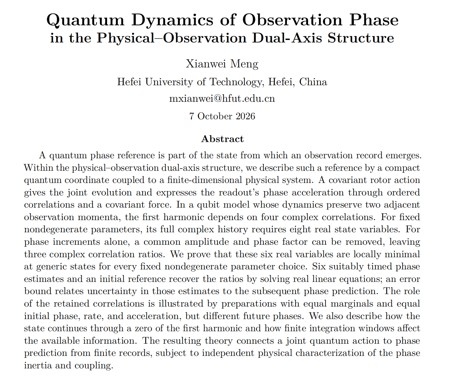
The exact amplitude, phase rate, and phase acceleration are

$$\begin{array}{cc}\hfill R\left(t\right)& =\frac{1}{2}\sqrt{D\left(t\right)},\hfill \end{array}$$

(38)

$$\begin{array}{cc}\hfill \dot{\phi }\left(t\right)& ={\displaystyle \frac{{\omega }_R}{2}}-{\displaystyle \frac{\kappa {\omega }_{R}z}{D\left(t\right)}},\hfill \end{array}$$

(39)

$$\begin{array}{cc}\hfill \ddot{\phi }\left(t\right)& =-{\displaystyle \frac{{\kappa }^2{\omega }_R^{2}z(1-z^2)sin\left(2u\right)}{D{\left(t\right)}^2}}.\hfill \end{array}$$

(40)

Although Q and ${\sigma }_z$ are conserved, the two conditional coherences accumulate different phases. Their sum produces the time-dependent rate in Eq. (39). Assigning the phase velocity corresponding to the mean polarization would lose this interference.

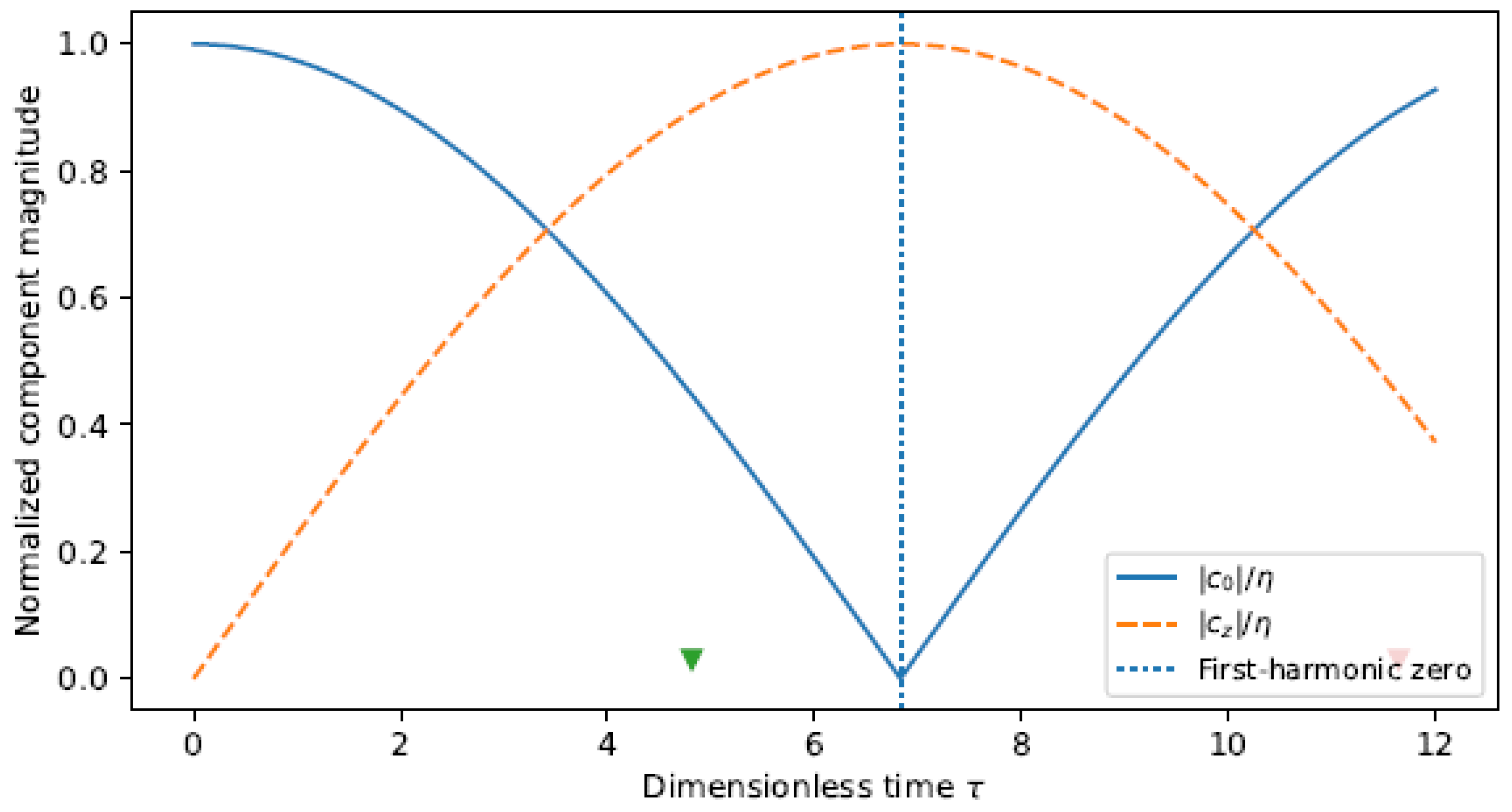
For $z=0$, c first vanishes at

$$t_{*}={\displaystyle \frac{\pi }{2\left|\kappa \right|{\omega }_R}},\kappa \ne 0.$$

(41)

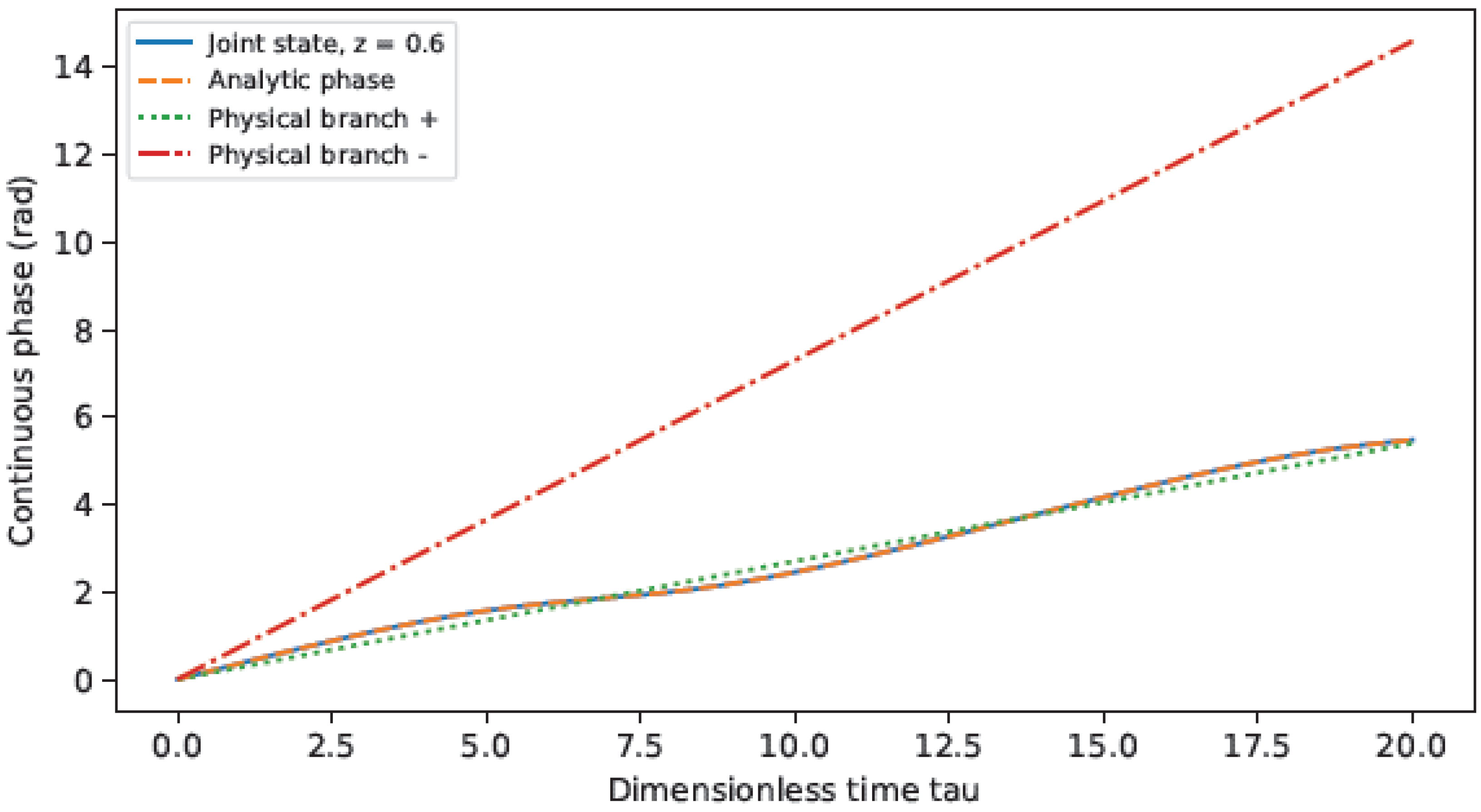
The first-harmonic contrast $2\left|c\right|$ subsequently revives, while the joint state remains a smooth superposition of four energy eigenstates throughout. For this two-momentum preparation, the phase distribution is

$$p_S(\chi ,t)={\displaystyle \frac{1}{2\pi }}\left[1+2Re\left(c\left(t\right)e^{-\mathrm{i}\chi }\right)\right],$$

(42)

and becomes uniform when $c=0$. Higher-momentum preparations can have nonzero higher harmonics even when their first moment vanishes.

Figure 1. Observation phase for $\kappa =0.23$, ${\omega }_X/{\omega }_R=0.7$, and $z=0.6$, alongside the two physical eigenstate preparations. Time is $\tau ={\omega }_{R}t$. Spectral evolution and Eq. (36) give coincident curves.

Figure 1. Observation phase for $\kappa =0.23$, ${\omega }_X/{\omega }_R=0.7$, and $z=0.6$, alongside the two physical eigenstate preparations. Time is $\tau ={\omega }_{R}t$. Spectral evolution and Eq. (36) give coincident curves.

4.4. Reciprocal Physical Coherence and Purity

Let $r_{+-}\left(t\right)=\langle +|{\rho }_X\left(t\right)|-\rangle$. For the product initial state above,

$$r_{+-}\left(t\right)=r_{+-}\left(0\right)e^{-\mathrm{i}{\omega }_{X}t}{e}^{\mathrm{i}u}cosu.$$

(43)

The observation momentum therefore modulates physical coherence, just as the physical preparation changes observation phase. For the pure initial physical state (35),

$$Tr{\rho }_X{\left(t\right)}^2=1-{\displaystyle \frac{1-z^2}{2}}{sin}^{2}u={\displaystyle \frac{1+{4\left|c\left(t\right)\right|}^2}{2}}.$$

(44)

For the balanced pure preparation, the first zero of c coincides with $Tr{\rho }_X^2=1/2$. The joint state is still pure: the reduced mixing arises from entanglement and later reverses. Equation (44) relies on the stated pure product preparation and two-momentum support.

Figure 2. First-harmonic contrast and physical reduced purity. For $z=0$, the first harmonic vanishes periodically; for $z=0.6$, $\left|c\right|\ge 0.3$. The curves satisfy Eq. (44) for the pure product preparations used here.

Figure 2. First-harmonic contrast and physical reduced purity. For $z=0$, the first harmonic vanishes periodically; for $z=0.6$, $\left|c\right|\ge 0.3$. The curves satisfy Eq. (44) for the pure product preparations used here.

4.5. Holonomy and Boundary Conditions

For Eq. (28), ${\mathcal{A}}_{\chi }=-\mathrm{i}\kappa {\sigma }_z$ is locally removable, but its holonomy is

$$\mathcal{W}=exp\left(-{\int }_0^{2\pi }{\mathcal{A}}_{\chi }\mathrm{d}\chi \right)=e^{2\pi \mathrm{i}\kappa {\sigma }_z}.$$

(45)

The transformation $G\left(\chi \right)=e^{-\mathrm{i}\kappa \chi {\sigma }_z}$ removes the connection locally. Unless $\kappa \in \mathbb{Z}$, it changes periodic wavefunctions into ones satisfying

$${\mathsf{\Psi }}^{\prime }(\chi +2\pi )=e^{-2\pi \mathrm{i}\kappa {\sigma }_z}{\mathsf{\Psi }}^{\prime }\left(\chi \right).$$

(46)

The connection has been transferred to the boundary condition. For integer $\kappa$, a periodic unitary removes it, but also transforms the preparation. Holding the original product preparation fixed after that transformation would define a different experiment. The holonomy here belongs to the quantum connection over $S^1$; the scalar response c still has the flat phase form described above.

5. The Correlations That Determine Phase

Initial correlations can affect reduced quantum evolution [14]. For the momentum-preserving branch of the present action, the correlations relevant to the first harmonic can be isolated exactly.

5.1. Equal Marginals and Different Futures

For the model (28), partial tracing of Eq. (11) gives

$${\dot{\rho }}_S=-{\displaystyle \frac{\mathrm{i}}{\hslash }}\left[{\displaystyle \frac{Q^2}{2\mathcal{I}}},{\rho }_S\right]+{\displaystyle \frac{\mathrm{i}\kappa }{\mathcal{I}}}[Q,{\rho }_z],{\rho }_z={Tr}_X\left[({\sigma }_z\otimes I_S)\varrho \right].$$

(47)

The extra operator ${\rho }_z$ records a joint correlation. Replacing it by $z{\rho }_S$ would close the reduced equation only by making an additional factorization assumption. The following pair makes the missing information visible in the phase.

Proposition 1

(Identical marginals can have different phase futures). For $\kappa \ne 0$, there are two states with identical ${\rho }_X$, identical ${\rho }_S$, and identical nonzero $c\left(0\right)$, but different initial observation-phase rates under the same Hamiltonian (28).

Proof. 

Let

$$|{\eta }_a\rangle ={\displaystyle \frac{|0\rangle +|1\rangle }{\sqrt{2}}},|{\eta }_b\rangle =\sqrt{0.9}|0\rangle +\sqrt{0.1}|1\rangle ,{\rho }_a=|{\eta }_a\rangle \langle {\eta }_a|,{\rho }_b=|{\eta }_b\rangle \langle {\eta }_b|.$$

(48)

Take the two correlated, separable preparations

$$\begin{array}{cc}\hfill {\varrho }_1& =\frac{1}{2}|+\rangle \langle +|\otimes {\rho }_a+\frac{1}{2}|-\rangle \langle -|\otimes {\rho }_b,\hfill \end{array}$$

(49)

$$\begin{array}{cc}\hfill {\varrho }_2& =\frac{1}{2}|+\rangle \langle +|\otimes {\rho }_b+\frac{1}{2}|-\rangle \langle -|\otimes {\rho }_a.\hfill \end{array}$$

(50)

Both have ${\rho }_X=I_X/2$ and ${\rho }_S=({\rho }_a+{\rho }_b)/2$. Since $Tr\left({\rho }_{a}E\right)=0.5$ and $Tr\left({\rho }_{b}E\right)=0.3$, both initial coherences equal $0.4$. Their evolutions are

$$\begin{array}{cc}\hfill c_1\left(t\right)& =0.25e^{\mathrm{i}{\mathsf{\Omega }}_{+}t}+0.15e^{\mathrm{i}{\mathsf{\Omega }}_{-}t},\hfill \end{array}$$

(51)

$$\begin{array}{cc}\hfill c_2\left(t\right)& =0.15e^{\mathrm{i}{\mathsf{\Omega }}_{+}t}+0.25e^{\mathrm{i}{\mathsf{\Omega }}_{-}t}.\hfill \end{array}$$

(52)

Therefore

$${\dot{\phi }}_1\left(0\right)={\omega }_R\left(\frac{1}{2}-\frac{\kappa }{4}\right),{\dot{\phi }}_2\left(0\right)={\omega }_R\left(\frac{1}{2}+\frac{\kappa }{4}\right).$$

(53)

Their difference is $\kappa {\omega }_R/2$, proving the assertion.    □

No entanglement is needed for this difference. The two preparations are separable, but pair the same sector states in different ways. Those pairings survive in the joint state and lead to distinct phase futures.

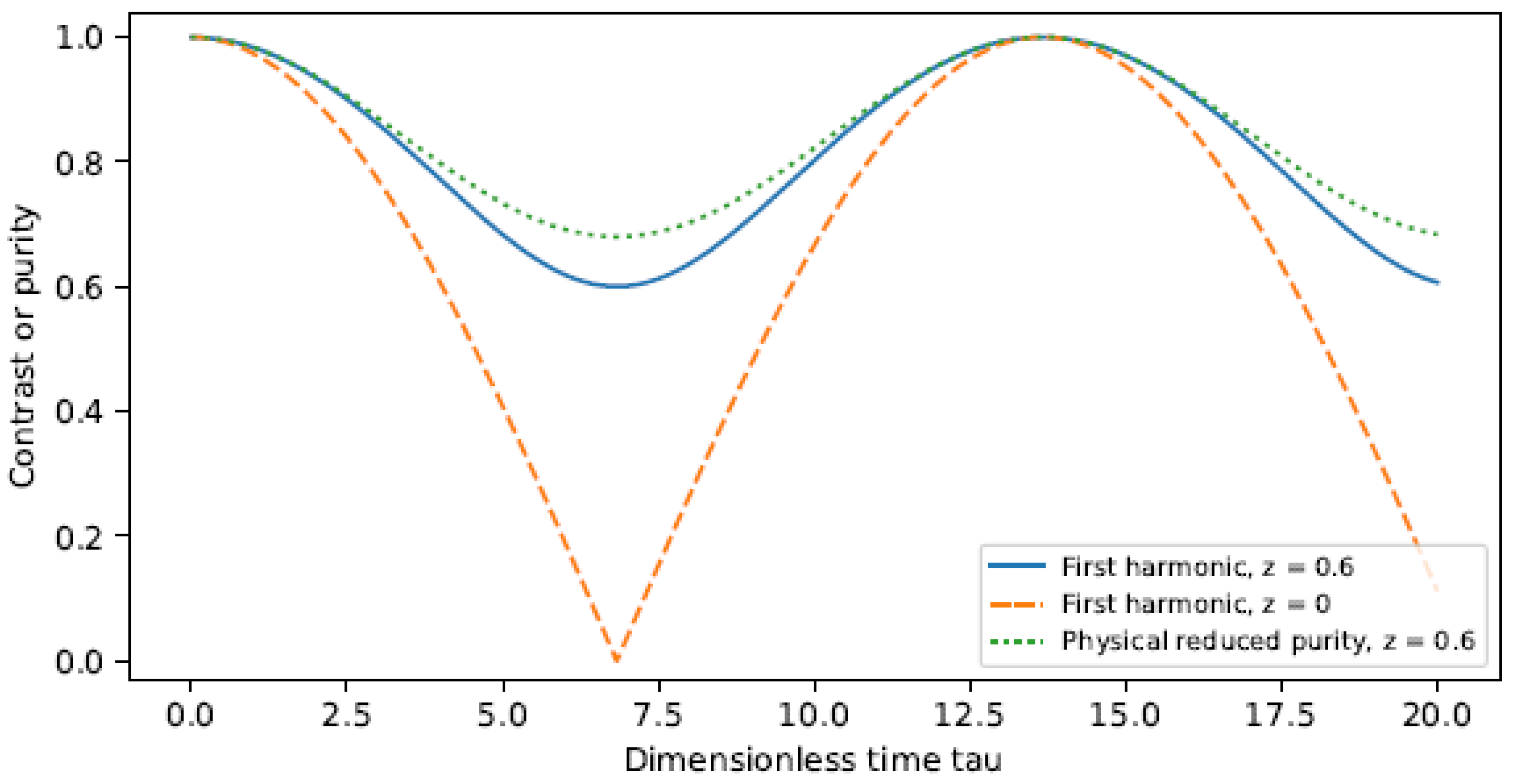
Writing $p\left(\varrho \right)=({\rho }_X,{\rho }_S)$, we have $p\left({\varrho }_1\right)=p\left({\varrho }_2\right)$ but different future readouts. Any deterministic predictor initialized only from $p\left(\varrho \right)$ must assign the same future to both and therefore fails on this pair. To retain just the information needed by the first harmonic, we now resolve the joint state into adjacent momentum blocks.

Figure 3. Phase histories of the two preparations in Eq. (50), with $\kappa =0.23$. Both start at $c\left(0\right)=0.4$ and have equal marginals, but their different correlations give initial dimensionless phase rates of $0.4425$ and $0.5575$.

Figure 3. Phase histories of the two preparations in Eq. (50), with $\kappa =0.23$. Both start at $c\left(0\right)=0.4$ and have equal marginals, but their different correlations give initial dimensionless phase rates of $0.4425$ and $0.5575$.

5.2. Adjacent Momentum Blocks

Suppose a and W are independent of $\chi$. The canonical observation momentum is then conserved, and the Hamiltonian has the block form

$$\mathsf{H}=\sum _{n\in \mathbb{Z}}{H}_n\otimes |n\rangle \langle n|,H_n={\displaystyle \frac{{(\hslash n{I}_X-a)}^2}{2\mathcal{I}}}+W.$$

(54)

Define the physical operator carried by adjacent observation momenta as

$${\mathsf{R}}_n=(I_X\otimes \langle n|)\varrho (I_X\otimes |n+1\rangle ).$$

(55)

This off-diagonal block need be neither Hermitian nor positive, although the density operator containing it is positive. Projecting the von Neumann equation onto the two momenta gives

$$\mathrm{i}\hslash {\dot{\mathsf{R}}}_n=H_n{\mathsf{R}}_n-{\mathsf{R}}_n{H}_{n+1},{\mathsf{R}}_n\left(t\right)=U_n\left(t\right){\mathsf{R}}_n\left(0\right)U_{n+1}{\left(t\right)}^{†},$$

(56)

where $U_n\left(t\right)=e^{-\mathrm{i}{H}_{n}t/\hslash }$. For finite momentum support,

$$c\left(t\right)=\sum _n{Tr}_X{\mathsf{R}}_n\left(t\right).$$

(57)

For a positive trace-class state, the sum is absolutely convergent. Positivity bounds each block contribution by the geometric mean of its two momentum populations, and the sum of these bounds is at most one.

The first harmonic thus depends only on adjacent blocks, each of which evolves independently of the nonadjacent ones. The hierarchy remains unbounded over arbitrary momentum preparations. An invariant preparation sector, however, can reduce it exactly.

We now retain the observation subspace

$${\mathcal{H}}_{01}=span\{|0\rangle ,|1\rangle \},P_{01}=|0\rangle \langle 0|+|1\rangle \langle 1|.$$

(58)

Because $[\mathsf{H},I_X\otimes P_{01}]=0$, a state prepared in this subspace remains there. Its phase moment can be evaluated with the compression $E_{01}=|1\rangle \langle 0|$, which has the same expectation as the full rotor shift on these states. Although $E_{01}$ is not unitary, no change to the full rotor algebra is involved. A term such as $vcos\chi$ would couple other momenta and require a return to the full dynamics of Section 3.

5.3. Four Joint Coherences for a Noncommuting Physical Generator

Keep the connection $a=\hslash \kappa {\sigma }_z$, but allow a transverse physical generator:

$$W={\displaystyle \frac{\hslash }{2}}({\omega }_x{\sigma }_x+{\omega }_z{\sigma }_z),\gamma =\kappa {\omega }_R,{\omega }_c={\displaystyle \frac{{\omega }_R}{2}},{\overline{\omega }}_z={\omega }_z-\gamma .$$

(59)

Here ${\omega }_R=\hslash /\mathcal{I}$, as before. On ${\mathcal{H}}_X\otimes {\mathcal{H}}_{01}$ there is one adjacent block $\mathsf{R}={\mathsf{R}}_0$. Expand it in the physical Pauli basis:

$$\mathsf{R}={\displaystyle \frac{1}{2}}\left(c_0{I}_X+c_x{\sigma }_x+c_y{\sigma }_y+c_z{\sigma }_z\right),c_{\mu }=Tr\left[\varrho ({\sigma }_{\mu }\otimes E)\right],{\sigma }_0=I_X.$$

(60)

The coefficient $c_0$ is the observed first harmonic. The other three coefficients retain the physical–observation correlations that the two marginals leave undetermined.

Theorem 3

(Exact finite correlation dynamics). For the momentum-preserving Hamiltonian (54) with coefficients (59), every initial joint state supported on ${\mathcal{H}}_X\otimes {\mathcal{H}}_{01}$ has moments satisfying

$$\begin{array}{cc}\hfill {\dot{c}}_0& =\mathrm{i}{\omega }_c{c}_0-\mathrm{i}\gamma c_z,\hfill \\ \hfill {\dot{c}}_x& =\mathrm{i}{\omega }_c{c}_x-{\overline{\omega }}_z{c}_y,\hfill \\ \hfill {\dot{c}}_y& =\mathrm{i}{\omega }_c{c}_y+{\overline{\omega }}_z{c}_x-{\omega }_x{c}_z,\hfill \\ \hfill {\dot{c}}_z& =\mathrm{i}{\omega }_c{c}_z+{\omega }_x{c}_y-\mathrm{i}\gamma c_0.\hfill \end{array}$$

(61)

Their initial values determine the complete future complex readout $c\left(t\right)$. For time-independent parameters, ${\sum }_{\mu =0,x,y,z}{\left|c_{\mu }\right|}^2$ is conserved.

Proof. 

Write $K=(H_0+H_1)/2$ and $\mathsf{\Delta }H=H_1-H_0$. Up to a scalar commuting with $\mathsf{R}$,

$$K={\displaystyle \frac{\hslash }{2}}({\omega }_x{\sigma }_x+{\overline{\omega }}_z{\sigma }_z),\mathsf{\Delta }H=\hslash ({\omega }_c{I}_X-\gamma {\sigma }_z).$$

Equation (56) becomes

$$\dot{\mathsf{R}}=-{\displaystyle \frac{\mathrm{i}}{\hslash }}[K,\mathsf{R}]+{\displaystyle \frac{\mathrm{i}}{2\hslash }}\{\mathsf{\Delta }H,\mathsf{R}\}.$$

(62)

The Pauli commutator supplies the rotation $({\omega }_x,0,{\overline{\omega }}_z)\times (c_x,c_y,c_z)$, while the anticommutator couples $c_0$ to $c_z$. Taking the four Pauli traces gives Eq. (61). Its constant matrix generator M is anti-Hermitian, so $\mathrm{d}\left({\mathit{c}}^{†}\mathit{c}\right)/\mathrm{d}t=0$. Equivalently, the left and right unitary factors in Eq. (56) preserve $Tr{\mathsf{R}}^{†}\mathsf{R}$.    □

The first equation relates the observation-phase rate to a physical–observation correlation. Wherever $c_0\ne 0$,

$$\dot{\phi }={\omega }_c-\gamma Re{\displaystyle \frac{c_z}{c_0}},{\displaystyle \frac{\dot{R}}{R}}=\gamma Im{\displaystyle \frac{c_z}{c_0}}.$$

(63)

For ${\omega }_x=0$, the pair $(c_0,c_z)$ closes. It still retains a correlation that the substitution $c_z=\langle {\sigma }_z\rangle c_0$ would discard. A nonzero ${\omega }_x$ brings $c_y$ into the evolution of $c_z$; a nonzero ${\overline{\omega }}_z$ then brings in $c_x$. The phase record can therefore draw on all four complex coefficients.

The same chain appears in the reciprocal force. In this branch, $F_{\mathsf{\Pi }}=-\hslash \kappa {\omega }_x{\sigma }_y$. Consequently,

$${\ddot{c}}_0=-({\omega }_c^2+{\gamma }^2)c_0+2{\omega }_c\gamma c_z-\mathrm{i}\gamma {\omega }_x{c}_y.$$

(64)

The $c_y$ term is the covariant-force contribution already present in Eq. (21). The moment system preserves it under reduction to the first harmonic.

5.4. A Fourth-Order Equation for the First Harmonic

For constant parameters, introduce $\mathcal{D}=\mathrm{d}/\mathrm{d}t-\mathrm{i}{\omega }_c$. Repeated differentiation of the first equation in (61) yields

$$\left[{\mathcal{D}}^4+({\gamma }^2+{\omega }_x^2+{\overline{\omega }}_z^2){\mathcal{D}}^2+{\gamma }^2{\overline{\omega }}_z^2\right]c_0=0.$$

(65)

Equation (65) governs the complex coherence and remains regular at its zeros. Its four complex initial data encode the same evolution as the correlation system.

When $\gamma {\omega }_x{\overline{\omega }}_z\ne 0$, the correlations can be recovered algebraically from the complex readout jet:

$$\begin{array}{cc}\hfill c_z& ={\displaystyle \frac{\mathrm{i}}{\gamma }}\mathcal{D}{c}_0,\hfill \\ \hfill c_y& ={\displaystyle \frac{\mathrm{i}}{\gamma {\omega }_x}}({\mathcal{D}}^2+{\gamma }^2)c_0,\hfill \\ \hfill c_x& ={\displaystyle \frac{\mathrm{i}}{\gamma {\omega }_x{\overline{\omega }}_z}}[{\mathcal{D}}^3+({\gamma }^2+{\omega }_x^2)\mathcal{D}]c_0.\hfill \end{array}$$

(66)

These identities express the correlations in terms of the complex readout and its first three covariant time derivatives. They will be used to establish minimality; finite-record reconstruction below avoids differentiating measured data.

Proposition 2

(Local minimality for the complex first harmonic). For fixed parameters with $\gamma {\omega }_x{\overline{\omega }}_z\ne 0$, four complex moments, or eight real variables, are necessary and sufficient for a smooth exact realization of all complex-readout histories on an open set of joint preparations supported on ${\mathcal{H}}_X\otimes {\mathcal{H}}_{01}$.

Proof. 

Let $\mathsf{A}=M-\mathrm{i}{\omega }_c{I}_4$. The map from $\mathit{c}={(c_0,c_x,c_y,c_z)}^{\mathsf{T}}$ to $(c_0,\mathcal{D}{c}_0,{\mathcal{D}}^2{c}_0,{\mathcal{D}}^3{c}_0)$ has matrix

$$\mathcal{O}=\left(\begin{array}{cccc}1& 0& 0& 0\\ 0& 0& 0& -\mathrm{i}\gamma \\ -{\gamma }^2& 0& -\mathrm{i}\gamma {\omega }_x& 0\\ 0& -\mathrm{i}\gamma {\omega }_x{\overline{\omega }}_z& 0& \mathrm{i}\gamma ({\gamma }^2+{\omega }_x^2)\end{array}\right),det\mathcal{O}=-\mathrm{i}{\gamma }^3{\omega }_x^2{\overline{\omega }}_z.$$

(67)

The matrix is invertible over $\mathbb{C}$, so the corresponding real map has rank eight. All eight directions are allowed by positivity: in momentum-block order, choose diagonal blocks $I_X/4$ and off-diagonal blocks $\mathsf{R},{\mathsf{R}}^{†}$. The resulting normalized density operator is strictly positive for ${\parallel \mathsf{R}\parallel }_{\mathrm{op}}<1/4$, allowing arbitrary small changes of the four complex coefficients. Any smooth realization of their full complex histories must reproduce the first three derivatives and hence have initialization rank at least eight. The four-moment system realizes this bound.    □

The count includes amplitude as well as phase. In the commuting case ${\omega }_x=0$, $\gamma \ne 0$, only two complex observable directions remain. There are three when ${\overline{\omega }}_z=0$ and $\gamma {\omega }_x\ne 0$, because $c_x$ decouples. At $\gamma =0$, only the single complex mode ${\dot{c}}_0=\mathrm{i}{\omega }_c{c}_0$ remains. We next remove the common complex scale to find the smaller state needed for phase increments.

6. The Minimal State for Phase Prediction

Multiplying all four correlations by the same nonzero complex number changes the initial amplitude and phase, but not the subsequent phase increments. Removing this scale leaves the relative correlations. The reduction concerns what the chosen record can reveal; it leaves the two PODA state roles unchanged.

6.1. The Projective Correlation State

Fix the autonomous parameters and the invariant observation support ${\mathcal{H}}_{01}$. For an initial moment vector $\mathit{c}$ with $c_0\ne 0$, define

$${\mathsf{\Gamma }}_{\mathit{c}}\left(t\right)={\displaystyle \frac{c_0\left(t\right)}{|c_0\left(t\right)|}}{\displaystyle \frac{|c_0\left(0\right)|}{c_0\left(0\right)}}.$$

(68)

We first compare phase histories on the connected nonzero-readout interval containing the initial time. Two states are locally equivalent when their factors agree near that time, that is, when their phase-history germs agree. To compare beyond later zeros, the recorded behavior must also include the zero times and the convention for continuing the reference.

Linearity implies $\mathit{c}(t;{\lambda }_0\mathit{c})={\lambda }_0\mathit{c}(t;\mathit{c})$ for any constant ${\lambda }_0\in \mathbb{C}\setminus \left\{0\right\}$. Hence Eq. (68) depends only on the correlation line $\left[\mathit{c}\right]\in {\mathbb{CP}}^3$. This line is a predictive state, not a pure-state ray of the density operator. Rescaling it need not preserve the same physical preparation, or even positivity at every magnitude.

Every correlation line has a physically admissible representative at a sufficiently small coherence magnitude. In momentum-block order, take

$${\varrho }_{\eta ,\mathit{r}}=\left(\begin{array}{cc}{I}_X/4& {\mathsf{R}}_{\eta ,\mathit{r}}\\ {\mathsf{R}}_{\eta ,\mathit{r}}^{†}& I_X/4\end{array}\right),{\mathsf{R}}_{\eta ,\mathit{r}}={\displaystyle \frac{\eta }{2}}(I_X+r_x{\sigma }_x+r_y{\sigma }_y+r_z{\sigma }_z).$$

(69)

Choosing $\eta >0$ small enough makes $\parallel {\mathsf{R}}_{\eta ,\mathit{r}}{\parallel }_{\mathrm{op}}<1/4$, so ${\varrho }_{\eta ,\mathit{r}}$ is strictly positive and has unit trace. Its moments are $\eta (1,r_x,r_y,r_z)$. One fixed choice of $\eta$ works in a neighborhood of any finite $\mathit{r}$, establishing that all six real ratio directions correspond to admissible quantum preparations.

On the chart $c_0\ne 0$, the projective coordinates are

$$r_x={\displaystyle \frac{c_x}{c_0}},r_y={\displaystyle \frac{c_y}{c_0}},r_z={\displaystyle \frac{c_z}{c_0}}.$$

(70)

The quotient rule applied to (61) yields

$$\begin{array}{cc}\hfill {\dot{r}}_x& =-{\overline{\omega }}_z{r}_y+\mathrm{i}\gamma r_x{r}_z,\hfill \\ \hfill {\dot{r}}_y& ={\overline{\omega }}_z{r}_x-{\omega }_x{r}_z+\mathrm{i}\gamma r_y{r}_z,\hfill \\ \hfill {\dot{r}}_z& ={\omega }_x{r}_y-\mathrm{i}\gamma +\mathrm{i}\gamma r_z^2,\hfill \\ \hfill \dot{\phi }& ={\omega }_c-\gamma Re{r}_z.\hfill \end{array}$$

(71)

The three complex ratios and their equations already suffice for the phase increments: once the initial reference is supplied, the last line gives the phase. This is a six-real-dimensional upper bound. The amplitude, when required, is recovered from

$${\displaystyle \frac{\mathrm{d}}{\mathrm{d}t}}log\left|c_0\right|=\gamma Im{r}_z.$$

(72)

Locally, the full eight-real-dimensional readout state consists of six ratio coordinates, an initial phase, and a positive amplitude scale.

Differentiating the phase rate shows how the remaining correlations enter:

$$\ddot{\phi }=-\gamma {\omega }_{x}Re{r}_y+{\gamma }^{2}Im\left(r_z^2\right).$$

(73)

The $r_y$ term carries the transverse physical evolution into phase acceleration. The quadratic term comes from dividing by the evolving readout. Both are consequences of the original linear correlation system.

6.2. Normalized Derivatives of the Carrier-Removed Coherence

The lower bound is easier to see after removing the known carrier. Set

$$z\left(t\right)=e^{-\mathrm{i}{\omega }_{c}t}{c}_0\left(t\right),\mathfrak{k}={\gamma }^2+{\omega }_x^2+{\overline{\omega }}_z^2,\mathfrak{l}={\gamma }^2{\overline{\omega }}_z^2.$$

(74)

The carrier-removed coherence obeys $z^{\left(4\right)}+\mathfrak{k}{z}^{\prime \prime }+\mathfrak{l}z=0$. On $z\ne 0$, divide its first three derivatives by z:

$$u_1={\displaystyle \frac{z^{\prime }}{z}},u_2={\displaystyle \frac{z^{\prime \prime }}{z}},u_3={\displaystyle \frac{z^{\prime \prime \prime }}{z}}.$$

(75)

Primes denote ordinary time derivatives for now; the rank calculation below uses dimensionless time. Differentiating these normalized derivatives gives

$${\dot{u}}_1=u_2-u_1^2,{\dot{u}}_2=u_3-u_2{u}_1,{\dot{u}}_3=-\mathfrak{k}{u}_2-\mathfrak{l}-u_3{u}_1,\dot{\phi }={\omega }_c+Im{u}_1.$$

(76)

The change from the physical–observation ratios is affine:

$$\begin{array}{cc}\hfill u_1& =-\mathrm{i}\gamma r_z,\hfill \\ \hfill u_2& =-{\gamma }^2-\mathrm{i}\gamma {\omega }_x{r}_y,\hfill \\ \hfill u_3& =-\mathrm{i}\gamma {\omega }_x{\overline{\omega }}_z{r}_x+\mathrm{i}\gamma ({\gamma }^2+{\omega }_x^2)r_z.\hfill \end{array}$$

(77)

The complex Jacobian determinant is $-\mathrm{i}{\gamma }^3{\omega }_x^2{\overline{\omega }}_z$, so the transformation is invertible when $\gamma {\omega }_x{\overline{\omega }}_z\ne 0$. Its inverse follows from Eq. (66) after normalization. In this branch, the normalized-derivative and correlation-ratio equations describe the same six-dimensional motion.

6.3. Minimality from Phase Derivatives

The upper bound counts sufficient coordinates. To prove that no smaller smooth state can reproduce the same phase histories, we examine derivatives of the output, as in local observability and realization theory [15,16].

For this calculation use $\tau =t/T_R$. Replace $\gamma ,{\omega }_x,{\overline{\omega }}_z,{\omega }_c$ by their dimensionless values and $u_j$ by $T_R^j{u}_j$, suppressing the bars. Write

$$U=(x_1,y_1,x_2,y_2,x_3,y_3)=(Re{u}_1,Im{u}_1,Re{u}_2,Im{u}_2,Re{u}_3,Im{u}_3).$$

(78)

Let f be the real vector field of (76), and let $h=y_1$ be the phase rate with the known carrier removed. Define

$${\mathcal{J}}_6=(h,L_{f}h,\dots ,L_f^{5}h),U_{*}=(0,0,0,0,0,1).$$

(79)

At this point, exact differentiation gives

$$D_U{\mathcal{J}}_6\left(U_{*}\right)=\left(\begin{array}{cccccc}0& 1& 0& 0& 0& 0\\ 0& 0& 0& 1& 0& 0\\ 0& 0& 0& 0& 0& 1\\ -4& 0& 0& -\mathfrak{k}& 0& 0\\ 0& 4\mathfrak{l}& -10& 0& 0& -\mathfrak{k}\\ 6\mathfrak{k}& 0& 0& {\mathfrak{k}}^2+14\mathfrak{l}& -20& 0\end{array}\right),det{D}_U{\mathcal{J}}_6\left(U_{*}\right)=-800.$$

(80)

Neither coefficient of the fourth-order equation appears in the determinant. Through the affine transformation, the test point corresponds to

$$r_{x,*}=-{\displaystyle \frac{1}{\gamma {\omega }_x{\overline{\omega }}_z}},r_{y,*}={\displaystyle \frac{\mathrm{i}\gamma }{{\omega }_x}},r_{z,*}=0,$$

(81)

The determinant in interleaved real ratio coordinates is $-800{\gamma }^6{\omega }_x^4{\overline{\omega }}_z^2$. By Eq. (69), the point and its neighborhood can be realized by positive joint states.

Theorem 4

(Local minimum for the observation-phase increment). Fix the autonomous Hamiltonian (54), the coefficients (59), and the invariant support ${\mathcal{H}}_X\otimes {\mathcal{H}}_{01}$, with $\gamma {\omega }_x{\overline{\omega }}_z\ne 0$. On an open dense set of the correlation chart $c_0\ne 0$, the local minimal smooth dynamical dimension for the phase-increment germ (68) is exactly six. The ratios (70) and their flow (71) attain this minimum. The initial phase is an independent reference, not one of the six increment states.

Proof. 

The ratio equations supply six real coordinates and hence the upper bound. For any fixed nondegenerate parameter triple, the affine map (77) is invertible. Equation (80) then makes ${\mathcal{J}}_6$ locally invertible at $U_{*}$. Equal phase-history germs have equal phase-rate derivatives through order five, so they have the same nearby ratio state.

Now consider any smooth m-dimensional deterministic realization, initialized by $s=p\left(U\right)$, that reproduces these phase increments. Its output derivatives define a smooth map ${\widehat{\mathcal{J}}}_6$ with ${\mathcal{J}}_6={\widehat{\mathcal{J}}}_6\circ p$. The chain rule gives $6=rankD{\mathcal{J}}_6\le m$. The positivity construction above ensures that this rank concerns allowed variations of the initial state.

For fixed parameters, $detD{\mathcal{J}}_6$ is a real polynomial in U. Since it is nonzero at $U_{*}$, its nonzero set is open and dense. The same local argument applies at every point of that set. Restoring physical units and the original coordinates preserves the rank.    □

The minimum is local to the stated invariant support and to the allowed family of initial states. It need not describe global phase equivalence, and further restrictions on preparation may lower it. Section 9 replaces the derivative argument by a reconstruction from finite phase values.

6.4. Lower-order branches and exceptional phase histories

The degenerate parameter cases have corresponding smaller phase realizations. If $\gamma \ne 0$ and ${\omega }_x=0$, the carrier-removed readout obeys $z^{\prime \prime }+{\gamma }^{2}z=0$. The complex variable $u=z^{\prime }/z$ satisfies $\dot{u}=-{\gamma }^2-u^2$, with phase rate ${\omega }_c+Imu$. The Jacobian of $(Imu,L_{f}Imu)$ with respect to $(Reu,Imu)$ has determinant $2Imu$, proving a generic two-real-state minimum.

If ${\overline{\omega }}_z=0$ and $\gamma {\omega }_x\ne 0$, the observable equation is $z^{\prime \prime \prime }+\mathfrak{k}{z}^{\prime }=0$. Its normalized state $(u_1,u_2)$ has four real components and evolves by

$${\dot{u}}_1=u_2-u_1^2,{\dot{u}}_2=-\mathfrak{k}{u}_1-u_2{u}_1.$$

(82)

The Jacobian of the phase rate and its first three derivatives has determinant $-18$ at $u_1=0$, $u_2=\mathrm{i}$. This gives a generic four-real-state minimum by the same argument. At $\gamma =0$, the phase rate is the known constant ${\omega }_c$, and no increment state is needed.

Table 1. Generic local dimensions on invariant two-momentum support. The phase origin is excluded from the increment column and included in the complex-readout column. Parameters are fixed and known.

Parameter branch	Complex readout	Phase increment
	(real states)	(real states)
$\gamma {\omega }_x{\overline{\omega }}_z\ne 0$	8	6
${\overline{\omega }}_z=0$, $\gamma {\omega }_x\ne 0$	6	4
${\omega }_x=0$, $\gamma \ne 0$	4	2
$\gamma =0$	2	0

Table 1. Generic local dimensions on invariant two-momentum support. The phase origin is excluded from the increment column and included in the complex-readout column. Parameters are fixed and known.

Parameter branch	Complex readout	Phase increment
	(real states)	(real states)
$\gamma {\omega }_x{\overline{\omega }}_z\ne 0$	8	6
${\overline{\omega }}_z=0$, $\gamma {\omega }_x\ne 0$	6	4
${\omega }_x=0$, $\gamma \ne 0$	4	2
$\gamma =0$	2	0

Special preparations also occur inside the nondegenerate parameter branch. Real initial values of $u_1,u_2,u_3$ remain real under Eq. (76). The ratio $z\left(t\right)/z\left(0\right)$ is then real, and while it stays positive the phase increment is just $e^{\mathrm{i}{\omega }_{c}t}$. Amplitudes can change along this three-dimensional real submanifold without changing the carrier-removed phase. All Lie derivatives of the corresponding phase rate vanish there. Their first three differentials nevertheless have an imaginary-coordinate minor of determinant one: the full codistribution has transverse rank three, while its restriction to the submanifold has rank zero. Different later zero times can still distinguish these histories.

7. Correlation-Sensitive Phase Preparations

7.1. Activating a Hidden Correlation

The correlation chain has a simple preparation-level consequence. Let ${\tau }_x=|0\rangle \langle 1|+|1\rangle \langle 0|$ act on the observation subspace, and consider

$${\varrho }_{\pm }={\displaystyle \frac{I_X\otimes I_{01}}{4}}+\alpha I_X\otimes {\tau }_x\pm \beta {\sigma }_y\otimes {\tau }_x,\alpha >0,\beta >0,\alpha +\beta <{\displaystyle \frac{1}{4}}.$$

(83)

These are normalized, strictly positive states. They are also separable: in the product eigenbasis of ${\sigma }_y$ and ${\tau }_x$, their probabilities are

$$p_{s,t}^{\pm }={\displaystyle \frac{1}{4}}+\alpha t\pm \beta st,s,t\in \{-1,1\}.$$

(84)

These probabilities give a direct preparation procedure: select physical ${\sigma }_y$ eigenstates and observation states $(|0\rangle \pm |1\rangle )/\sqrt{2}$ according to a classical record.

Both preparations have

$${\rho }_X={\displaystyle \frac{I_X}{2}},{\rho }_S={\displaystyle \frac{I_{01}}{2}}+2\alpha {\tau }_x,(c_0,c_x,c_y,c_z)\left(0\right)=(2\alpha ,0,\pm 2\beta ,0).$$

(85)

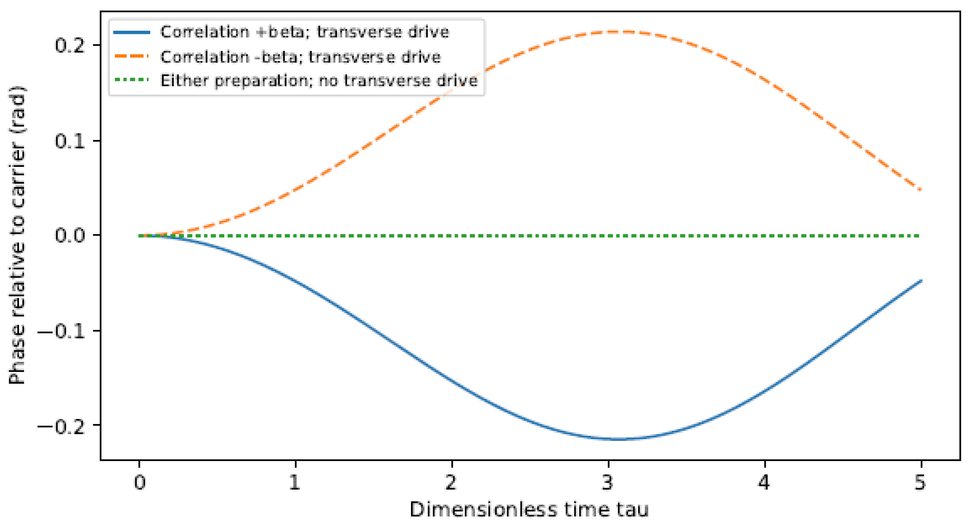
The marginals, the initial coherence, and its first derivative agree. The differing $c_y$ correlations first appear in the phase acceleration:

$$\begin{array}{cc}\hfill c_{0,+}\left(0\right)& =c_{0,-}\left(0\right)=2\alpha ,\hfill \\ \hfill {\dot{\phi }}_{+}\left(0\right)& ={\dot{\phi }}_{-}\left(0\right)={\omega }_c,\hfill \\ \hfill {\ddot{\phi }}_{\pm }\left(0\right)& =\mp \gamma {\omega }_x{\displaystyle \frac{\beta }{\alpha }}.\hfill \end{array}$$

(86)

The first two lines follow from $c_z\left(0\right)=0$; the third follows by inserting (85) into (64). With the common initial phase set to zero,

$${\phi }_{+}\left(t\right)-{\phi }_{-}\left(t\right)=-\gamma {\omega }_x{\displaystyle \frac{\beta }{\alpha }}{t}^2+O\left(t^4\right).$$

(87)

The cubic term vanishes for this preparation, since the first and third derivatives of $e^{-\mathrm{i}{\omega }_{c}t}{c}_0\left(t\right)$ vanish at the origin. The expansion concerns a neighborhood with nonzero coherence and a common continuous phase branch.

If the transverse generator is absent, the same two preparations instead give identical histories for all times:

$$c_{0,+}\left(t\right)=c_{0,-}\left(t\right)=2\alpha e^{\mathrm{i}{\omega }_{c}t}cos\left(\gamma t\right),{\omega }_x=0.$$

(88)

Without the transverse generator, the two $c_y$ correlations remain invisible to this phase record. A nonzero ${\omega }_x$ transfers their difference into $c_z$ and then into $c_0$, without changing the observable being read. For both preparations, the diagonal momentum blocks stay at $I_X/4$, so ${\rho }_X\left(t\right)=I_X/2$ throughout. The later phase separation therefore cannot be attributed to differing physical marginals.

For the dimensionless values

$$\alpha =0.10,\beta =0.05,\kappa =0.23,{\omega }_x{T}_R=0.9,{\omega }_z{T}_R=0.7,$$

(89)

where $T_R=\mathcal{I}/\hslash$, both initial phase rates are $0.5$ per unit $\tau =t/T_R$. Their initial phase accelerations are $-0.1035$ and $+0.1035$ per unit ${\tau }^2$, so the signed acceleration difference is $-0.207/T_R^2$ in physical time. The predicted phase separation begins as $-0.1035{\tau }^2$. Figure 4 shows the complete trajectories, not merely this local expansion.

The pair isolates one joint correlation under the same unitary dynamics. Conditional spectroscopy supplies $T_R$ and $\kappa$; independent characterization fixes the physical-generator components and preparation probabilities (84). With these quantities fixed, the acceleration contrast is a prediction rather than a fitted coefficient.

7.2. A Phase Difference first Appearing at Third Order

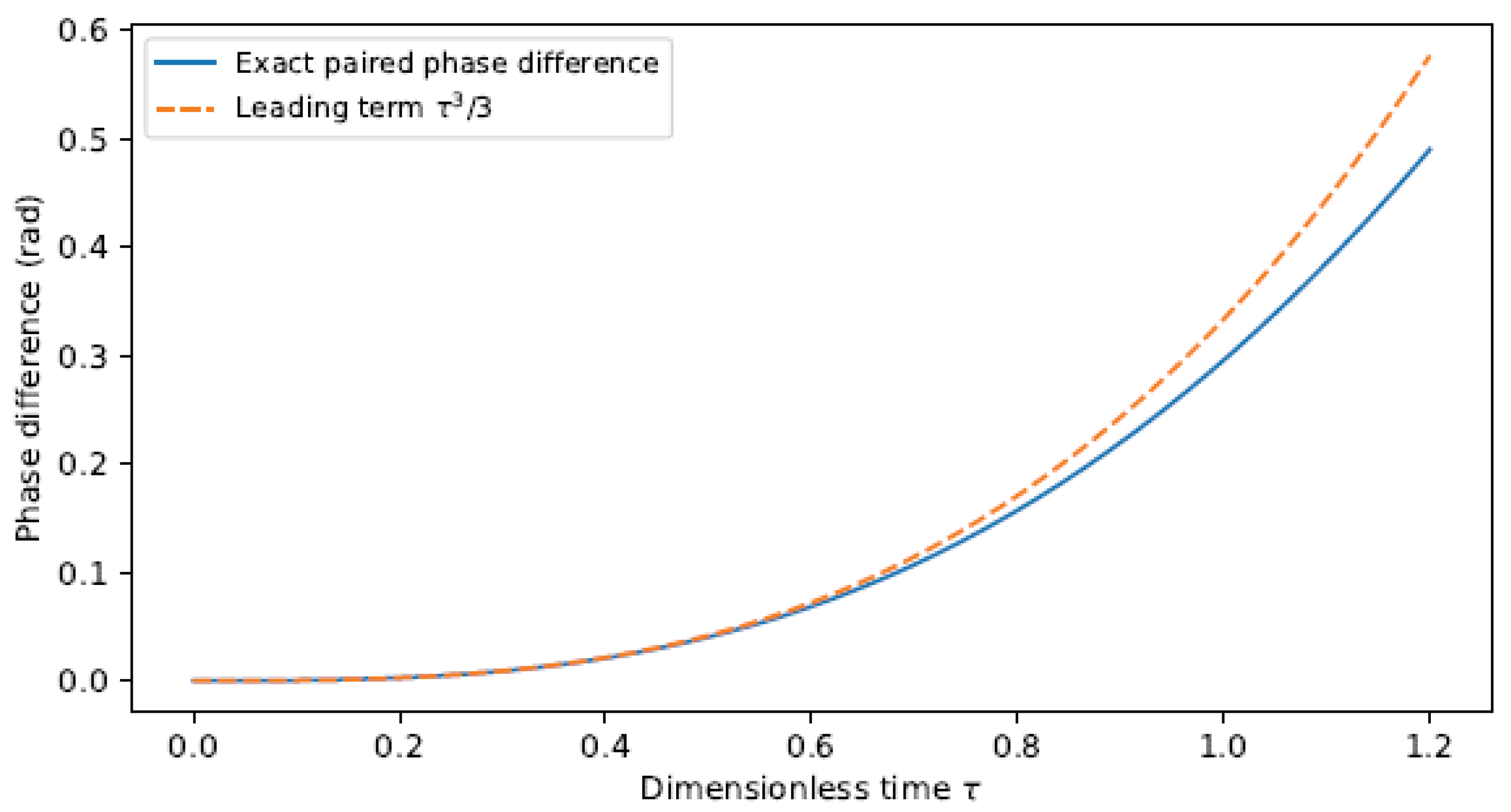
A second preparation pair postpones the phase difference to third order. Use dimensionless parameters $\gamma ={\omega }_x={\overline{\omega }}_z=1$ and ${\omega }_c=1/2$, so that $\mathfrak{k}=3$ and $\mathfrak{l}=1$. Choose

$${\mathit{c}}_{\pm }\left(0\right)=\eta (1,\mp 1,\mathrm{i},0),\eta =0.1,$$

(90)

and the positive density operators (69). Both physical marginals are $I_X/2$, and both observation marginals have diagonal entries $1/2$ and off-diagonal entry $\eta$. The joint states differ only in their correlations. Their smallest eigenvalue is $1/4-\eta (1+\sqrt{2})/2>0$.

Equation (77) gives $u_1=u_2=0$ and $u_3=\pm \mathrm{i}$. Hence

$${\phi }_{\pm }\left(0\right)=0,{\phi }_{\pm }^{\prime }\left(0\right)={\displaystyle \frac{1}{2}},{\phi }_{\pm }^{\prime \prime }\left(0\right)=0,{\phi }_{\pm }^{\prime \prime \prime }\left(0\right)=\pm 1.$$

(91)

Here and in the following expression, primes denote $\tau$ derivatives. The real-coefficient fourth-order equation makes the two carrier-removed coherences complex conjugates. Its even and odd solutions give

$${\phi }_{+}\left(\tau \right)-{\phi }_{-}\left(\tau \right)={\displaystyle \frac{{\tau }^3}{3}}-{\displaystyle \frac{\mathfrak{k}{\tau }^5}{60}}+O\left({\tau }^7\right).$$

(92)

Here even the initial phase acceleration fails to distinguish the two states. Their different third derivatives reveal correlations that the marginals and lower-order phase data conceal. The example rules out a closure in those data; the full six-dimensional lower bound follows from Theorem 4.

Figure 5. Third-order phase separation for the preparations in Eq. (90). Their initial phase, rate, acceleration, and marginals agree. The exact separation departs from the leading cubic term as the higher-order terms in Eq. (92) become appreciable.

Figure 5. Third-order phase separation for the preparations in Eq. (90). Their initial phase, rate, acceleration, and marginals agree. The exact separation departs from the leading cubic term as the higher-order terms in Eq. (92) become appreciable.

8. Phase Measurements and Readout Zeros

8.1. Joint Phase Records

The retained correlations can be read from joint measurements. Restricting the rotor phase spectral measure to ${\mathcal{H}}_{01}$ gives the positive operator-valued measure

$${\mathsf{M}}_{01}\left(\mathrm{d}\chi \right)={\displaystyle \frac{\mathrm{d}\chi }{2\pi }}\left(\begin{array}{cc}1& e^{\mathrm{i}\chi }\\ e^{-\mathrm{i}\chi }& 1\end{array}\right),{\int }_0^{2\pi }{\mathsf{M}}_{01}\left(\mathrm{d}\chi \right)=I_{01},{\int }_0^{2\pi }{e}^{\mathrm{i}\chi }{\mathsf{M}}_{01}\left(\mathrm{d}\chi \right)=E_{01}.$$

(93)

The compression preserves the phase probabilities of states in the invariant subspace. In two dimensions it is a positive operator-valued measure, rather than a projection-valued angle observable.

Choose a physical Pauli direction $a\in \{x,y,z\}$ and let $P_{a,s}=(I_X+s{\sigma }_a)/2$. Since the two measurements act on different tensor factors, their joint record is

$$p_a(s,\mathrm{d}\chi ;t)=Tr\left[\varrho \left(t\right)\left(P_{a,s}\otimes {\mathsf{M}}_{01}\left(\mathrm{d}\chi \right)\right)\right].$$

(94)

The moments follow from ordinary weighted averages:

$$c_0\left(t\right)=\sum _{s=\pm 1}\int e^{\mathrm{i}\chi }{p}_a(s,\mathrm{d}\chi ;t),c_a\left(t\right)=\sum _{s=\pm 1}s\int e^{\mathrm{i}\chi }{p}_a(s,\mathrm{d}\chi ;t).$$

(95)

Each Pauli setting uses a separately prepared ensemble, evolved freely to the chosen terminal time. The protocol therefore does not require simultaneous measurements of incompatible physical observables or continuous monitoring during the evolution.

For N independent terminal records in one setting, the sample mean of $s{e}^{\mathrm{i}\chi }$ is unbiased and satisfies

$$\mathbb{E}{\left|{\widehat{c}}_a-c_a\right|}^2={\displaystyle \frac{1-|c_a{|}^2}{N}}.$$

(96)

Each sample has unit modulus, which gives the variance identity. Instrument response and correlated preparation errors require a separate calibration model. Once the initial moments have been estimated, Eq. (61) predicts later complex records directly, avoiding high-order differentiation of measured phase.

8.2. Finite Integration Windows

Let all four moments be read through the same fixed, nonnegative, normalized integrable kernel $w\left(s\right)$ of compact support. At center times for which the full window is available,

$$\overline{\mathit{c}}\left(t\right)=\int w\left(s\right)\mathit{c}(t+s)\mathrm{d}s=F_w\left(M\right)\mathit{c}\left(t\right),F_w\left(M\right)=\int w\left(s\right)e^{Ms}\mathrm{d}s.$$

(97)

Since M is constant, it commutes with the window operator and $\dot{\overline{\mathit{c}}}=M\overline{\mathit{c}}$. The filtered moments obey the original correlation law, but start from filtered initial values.

For a rectangular window of width T, an eigenmode of M with eigenvalue $\mathrm{i}\nu$ is multiplied by $sinc(\nu T/2)$, where $sincx=sinx/x$. From (65), the four mode frequencies are

$$\begin{array}{c}\nu ={\omega }_c\pm {\mathsf{\Omega }}_{+},{\omega }_c\pm {\mathsf{\Omega }}_{-},\\ {\mathsf{\Omega }}_{\pm }^2={\displaystyle \frac{1}{2}}\left[K\pm \sqrt{K^2-4{\gamma }^2{\overline{\omega }}_z^2}\right],K={\gamma }^2+{\omega }_x^2+{\overline{\omega }}_z^2.\end{array}$$

(98)

The window map is invertible precisely when all retained modal factors are nonzero. A vanishing factor removes its mode from the entire filtered history, even if the instantaneous dynamics can distinguish it. Thus recovery depends on both the evolution and the readout window. Time-dependent generators, unequal kernels, or moving references require the corresponding measurement operator in place of this common fixed window.

8.3. Continuation Through Readout Zeros

The ratios become singular at a zero of $c_0$, but the correlation vector does not. Its norm is conserved by the anti-Hermitian generator M, so a nonzero vector always has a component that can serve as a new projective denominator.

On the chart $c_j\ne 0$, put $q_k^{\left(j\right)}=c_k/c_j$, with $q_j^{\left(j\right)}=1$. The chart flow and its reference phase are

$${\dot{q}}_k^{\left(j\right)}={\left(M{\mathit{q}}^{\left(j\right)}\right)}_k-q_k^{\left(j\right)}{\left(M{\mathit{q}}^{\left(j\right)}\right)}_j,{\dot{\varphi }}_j=Im{\left(M{\mathit{q}}^{\left(j\right)}\right)}_j.$$

(99)

At an overlap with $c_{\ell }\ne 0$, the transition is

$$q_k^{(\ell )}={\displaystyle \frac{q_k^{\left(j\right)}}{q_{\ell }^{\left(j\right)}}},{\varphi }_{\ell }={\varphi }_j+Arg{q}_{\ell }^{\left(j\right)}(mod2\pi ).$$

(100)

Whenever $c_0\ne 0$, the recorded phase is ${\varphi }_j+Arg{q}_0^{\left(j\right)}$. If the conserved norm $C=\parallel \mathit{c}\parallel$ is retained, the full moment vector is recovered as

$$\mathit{c}={\displaystyle \frac{C}{\parallel {\mathit{q}}^{\left(j\right)}\parallel }}{e}^{\mathrm{i}{\varphi }_j}{\mathit{q}}^{\left(j\right)}.$$

(101)

The projective state therefore continues through changes of chart, with the local reference phases related by Eq. (100). This continuation leaves $Arg{c}_0$ undefined at an exact readout zero. If every correlation vanishes initially, all remain zero; in that case there is neither a correlation line nor a first-harmonic phase.

For example, in the commuting branch, take $\mathit{c}\left(0\right)=(\eta ,0,0,0)$ with $0<\eta <1/2$. Then

$$c_0\left(t\right)=\eta e^{\mathrm{i}{\omega }_{c}t}cos\gamma t,c_z\left(t\right)=-\mathrm{i}\eta e^{\mathrm{i}{\omega }_{c}t}sin\gamma t.$$

(102)

At $t_{*}=\pi /\left(2\right|\gamma \left|\right)$ the first harmonic vanishes, while $|c_z|=\eta$. The ratio $c_0/c_z$ remains regular and carries the state through the zero. A subsequent phase comparison uses this continued complex state, leaving the phase at the zero unassigned.

8.4. Filtered Phase States and Measurement Precision

Because the common-window moments obey the same linear system, their ratios obey Eq. (71) wherever the filtered denominator is nonzero. The correct initial values are ratios of filtered moments, not filtered ratios. An invertible $F_w\left(M\right)$ preserves open sets of preparation coordinates and the generic six-state minimum. When a mode is suppressed, the minimum must be computed on the image of the window map.

For the parameters used in Appendix E, a rectangular window of width $0.6$ has a smallest modal-factor modulus of $0.96499$; the reduced calculation reproduces its first harmonic to $3.24\times {10}^{-15}$. A width of about $4.09111$ instead suppresses one mode completely. Changing projective coordinates cannot recover a mode removed by the window.

Removing the common amplitude is appropriate for ideal phase prediction, but not for assigning measurement precision. If the moment errors satisfy $|\delta c_0|\le {ϵ}_0<\left|c_0\right|$ and $|\delta c_a|\le {ϵ}_a$, then

$$\left|{\displaystyle \frac{c_a+\delta c_a}{c_0+\delta c_0}}-r_a\right|\le {\displaystyle \frac{{ϵ}_a+\left|r_a\right|{ϵ}_0}{|c_0|-{ϵ}_0}}.$$

(103)

A small denominator magnifies uncertainty in the ratios. In weak-coherence records it is therefore preferable to retain the complex moments and their error estimates, even when the ideal phase dynamics have a six-variable realization.

9. Reconstruction from Finite Phase Records

The minimal state has so far been characterized by its future phase derivatives. Measurements give phase values at finite times instead. With the generator known, those values impose linear constraints on the initial correlation ratios. We derive these constraints for identically prepared ensembles, each evolved under the same Hamiltonian and measured at its terminal time.

9.1. A linear inverse problem for the correlation ratios

Remove the known carrier from the four-moment generator and write

$$\mathsf{A}=M-\mathrm{i}{\omega }_c{I}_4,b\left(t\right)=e_0^{\mathsf{T}}{e}^{\mathsf{A}t}=(b_0\left(t\right),b_x\left(t\right),b_y\left(t\right),b_z\left(t\right)),d={(1,r_x,r_y,r_z)}^{\mathsf{T}}.$$

(104)

Here $e_0={(1,0,0,0)}^{\mathsf{T}}$, and the ratios refer to the initial time, now set to zero. The normalized coherence is

$$f(t;d)=b\left(t\right)d=e^{-\mathrm{i}{\omega }_{c}t}{\displaystyle \frac{c_0\left(t\right)}{c_0\left(0\right)}},f(0;d)=1.$$

(105)

Dividing by $c_0\left(0\right)$ removes the common amplitude and phase from the readout, without altering the density operator. At a time $t_j$ with nonzero coherence, the measured phase factor is

$${\zeta }_j=e^{-\mathrm{i}{\omega }_c{t}_j}{\mathsf{\Gamma }}_{\mathit{c}}\left(t_j\right)={\displaystyle \frac{f(t_j;d)}{\left|f\right(t_j;d\left)\right|}}.$$

(106)

Using the unit factors keeps the reconstruction independent of any choice of integer phase branch.

Let $v={(Re{r}_x,Im{r}_x,Re{r}_y,Im{r}_y,Re{r}_z,Im{r}_z)}^{\mathsf{T}}$. Each phase value gives

$$Im\left[{\overline{\zeta }}_{j}b\left(t_j\right)d\right]=0,Re\left[{\overline{\zeta }}_{j}b\left(t_j\right)d\right]>0.$$

(107)

The equality is linear in v. With $a_{ja}={\overline{\zeta }}_j{b}_a\left(t_j\right)$, define

$$\begin{array}{cc}\hfill {\left({\mathsf{K}}_{\zeta }\right)}_{j,:}& =(Im{a}_{jx},Re{a}_{jx},Im{a}_{jy},Re{a}_{jy},Im{a}_{jz},Re{a}_{jz}),\hfill \\ \hfill q_j& =-Im\left[{\overline{\zeta }}_j{b}_0\left(t_j\right)\right].\hfill \end{array}$$

(108)

The initial phase state is therefore obtained from

$${\mathsf{K}}_{\zeta }v=q.$$

(109)

The equalities require each predicted readout to lie on the measured phase line; the strict inequalities select its positive direction. They are checked after the solve. No absolute coherence magnitude or individual joint moment is needed as an input.

Theorem 5

(Reconstruction from six terminal phases). Let the generator be known, time independent, and in the nondegenerate two-momentum branch of Theorem 4. Let the terminal records share one initial ensemble and phase reference. If six nonzero readouts give a nonsingular ${\mathsf{K}}_{\zeta }$, their exact phase factors determine at most one ratio state in the chart $c_0\left(0\right)\ne 0$. For admissible data, Eq. (109) recovers that state, whose subsequent phase follows from Eq. (71) or Eq. (105). The reconstruction determines ratios, not the full density operator or absolute coherence magnitude.

At any full-rank point of the six-derivative map, six distinct positive times can be chosen in an arbitrarily short nonzero-readout interval to make the reconstruction locally regular. On a generic open set, fewer than six scalar terminal phases do not determine the phase future. The initial reference is additional to the six measurements.

Proof. 

Two states producing the same six phase factors satisfy the same real linear system. Nonsingularity makes their ratio coordinates equal. If the data arise from a nonzero trajectory, its solution also satisfies the directional inequalities.

For existence, use the canonical real coordinates U in (78). Let $\theta (t;U)=Argf(t;U)$ be the local lift with $\theta (0;U)=0$, and set $h=Im{u}_1$. Its Taylor expansion gives

$$D_U\theta (t;U)={\displaystyle \sum _{k=1}^6}{\displaystyle \frac{t^k}{k!}}{D}_U{L}_f^{k-1}h\left(U\right)+O\left(t^7\right).$$

For $t_j=j\delta$, multilinearity of the determinant and the Vandermonde identity yield

$$det{D}_U\left(\theta \left(\delta \right),\dots ,\theta \left(6\delta \right)\right)={\delta }^{21}det{D}_U{\mathcal{J}}_6\left(U\right)+O\left({\delta }^{22}\right).$$

(110)

Indeed, $1+\dots +6=21$ and $det{[j^k/k!]}_{j,k=1}^6=1$. The leading coefficient at $U_{*}$ is $-800$. More generally it is nonzero at every full-rank point. The affine coordinate change (77) is invertible, and differentiation of the measured argument gives

$${\mathsf{K}}_{\zeta }=diag\left(\right|f\left(t_1\right)|,\dots ,|f\left(t_6\right)\left|\right)D_v\left(\theta \left(t_1\right),\dots ,\theta \left(t_6\right)\right).$$

(111)

Thus ${\mathsf{K}}_{\zeta }$ is nonsingular for sufficiently small positive $\delta$. Local nonvanishing follows from $f\left(0\right)=1$.

With fewer than six phase values, the real system has a nontrivial kernel. Small displacements along that kernel preserve its equalities and the strict directional inequalities. They also remain physically admissible by (69). Near a full-rank phase-state point, distinct such states have different phase-history germs by Theorem 4. Hence the smaller set of records does not determine the generic future.    □

Invertibility depends on the preparation as well as the sampling times. Appendix D gives an algebraic example and a recurrent schedule that loses all six directions. Full rank alone does not guarantee a useful experiment: as the times coalesce, the determinant in Eq. (110) vanishes to order twenty-one, making the distinctions increasingly sensitive to noise.

9.2. Angular Errors and a Bound on the Recovered State

Additional phase records give an overdetermined version of the same inverse problem. Suppose ${\widehat{\zeta }}_j={\zeta }_j{e}^{\mathrm{i}{\delta }_j}$ with known bounds $|{\delta }_j|\le {ϵ}_j<\pi /2$. Form $\widehat{\mathsf{K}}$ and $\widehat{q}$ from the measured factors. When $\widehat{\mathsf{K}}$ has full column rank, the unweighted least-squares estimate is

$$\widehat{v}={\widehat{\mathsf{K}}}^{+}\widehat{q},\widehat{d}={(1,{\widehat{r}}_x,{\widehat{r}}_y,{\widehat{r}}_z)}^{\mathsf{T}}.$$

(112)

The superscript + denotes the Moore–Penrose inverse. Only the initial ratio state is estimated; the frequencies and coupling remain fixed.

Proposition 3

(A posteriori state-error bound). For the known anti-Hermitian generator $\mathsf{A}$, put

$$s_{ϵ}={\left(\sum _j{sin}^2{ϵ}_j\right)}^{1/2},{\sigma }_{*}={\sigma }_{min}\left(\widehat{\mathsf{K}}\right),b_{ϵ}={\displaystyle \frac{s_{ϵ}}{{\sigma }_{*}}}.$$

(113)

If $b_{ϵ}<1$, the estimated ratio state satisfies

$$\parallel \widehat{\mathit{r}}{-\mathit{r}\parallel }_2\le B_{ϵ}:={\displaystyle \frac{b_{ϵ}{\parallel \widehat{d}\parallel }_2}{1-b_{ϵ}}}.$$

(114)

No independence assumption on the phase errors is required.

Proof. 

Inserting the true state in the measured equations gives the residual

$$e_j={(\widehat{\mathsf{K}}v-\widehat{q})}_j=-\left|f(t_j;d)\right|sin{\delta }_j.$$

Since $e^{\mathsf{A}t}$ is unitary, $\parallel b\left(t_j\right){\parallel }_2=1$ and $|f(t_j;d){|\le \parallel d\parallel }_2$. Therefore ${\parallel e\parallel }_2\le s_{ϵ}{\parallel d\parallel }_2$. Full column rank implies $\widehat{v}-v=-{\widehat{\mathsf{K}}}^{+}e$, so $\parallel \widehat{v}{-v\parallel }_2\le b_{ϵ}{\parallel d\parallel }_2$. The real-coordinate norm equals the complex-ratio norm, and ${\parallel d\parallel }_2\le \parallel \widehat{d}{\parallel }_2+{\parallel \widehat{v}-v\parallel }_2$. Rearranging gives (114).    □

Reference uncertainty is common to every increment. If the absolute errors at zero and $t_j$ are bounded by $e_0$ and $e_j$, respectively, the choice ${ϵ}_j=e_0+e_j$ includes that shared error without assuming independence. The bound treats the generator and time scale as known. Their calibration errors must be propagated through the record equations before they can be included.

9.3. Prediction with a Nonzero-Readout Margin

Let $\widehat{f}\left(t\right)=b\left(t\right)\widehat{d}$ and $L\left(t\right)=\parallel (b_x\left(t\right),b_y\left(t\right),b_z\left(t\right)){\parallel }_2$. The recovered state predicts

$$\widehat{\mathsf{\Gamma }}\left(t\right)=e^{\mathrm{i}{\omega }_{c}t}{\displaystyle \frac{\widehat{f}\left(t\right)}{|\widehat{f}\left(t\right)|}}.$$

(115)

Equation (114) implies $|f\left(t\right)-\widehat{f}\left(t\right)|\le L\left(t\right)B_{ϵ}$. Whenever $L\left(t\right)B_{ϵ}<\left|\widehat{f}\left(t\right)\right|$, the disk of possible complex readouts excludes zero, and

$$\begin{array}{cc}\hfill \left|f\right(t\left)\right|& \ge |\widehat{f}\left(t\right)|-L\left(t\right)B_{ϵ}>0,\hfill \\ \hfill \left|Arg\left(\widehat{\mathsf{\Gamma }}\left(t\right)\overline{\mathsf{\Gamma }\left(t\right)}\right)\right|& \le arcsin{\displaystyle \frac{L\left(t\right)B_{ϵ}}{|\widehat{f}\left(t\right)|}}.\hfill \end{array}$$

(116)

Geometrically, the bound is the largest angle subtended by the error disk at the origin. It measures circular error, independently of integer unwrapping. The result assumes exact arithmetic; implementation errors in the propagator and linear solve require their own allowance.

A finite grid can also bound nonvanishing on a whole prediction interval. If the endpoints are included and the largest grid gap is $\mathsf{\Delta }t$, then $|\dot{\widehat{f}}|\le |\gamma |\parallel \widehat{d}{\parallel }_2$, since the first row of $\mathsf{A}$ has norm $\left|\gamma \right|$. Consequently,

$$\underset{t}{inf}\left|f\left(t\right)\right|\ge \underset{t_k}{min}\left|\widehat{f}\left(t_k\right)\right|-{\displaystyle \frac{\left|\gamma \right|\parallel \widehat{d}{\parallel }_2\mathsf{\Delta }t}{2}}-B_{ϵ}.$$

(117)

A positive lower bound ensures a continuous phase lift on the whole interval. Failure of the bound to be positive is inconclusive: it does not establish a zero. At an actual zero, only the correlation state continues, as described in Section 8.3.

9.4. Ensemble Readout and Visibility

A terminal phase is the argument of an estimated circular moment, so each of the six values is an ensemble statistic, not an individual quantum event. The ensembles share the same initial preparation and evolve freely under the same generator before being measured. The protocol contains no continuous measurement during that evolution.

Although only phase factors enter the inversion, coherence magnitudes and sample counts are needed to bound their angular errors. Weak first harmonics remain difficult to measure. Joint Pauli–phase records offer a second route to the initial ratios; the finite-time method instead uses the known dynamics to reveal those correlations in the phase history.

For a common fixed window, apply the construction to $\overline{\mathit{c}}$, which has the same generator. The recovered state and its predictions then refer to windowed readouts. Recovering the instantaneous correlations additionally requires an invertible window map; no phase inversion can restore a mode that the window has removed.

10. Experimental Implications

One set of calibrated parameters determines the conditional splitting (34), the coherence envelope (36), and the correlation-sensitive contrasts of Section 7. For the pure product preparation, Eq. (44) also relates the observation contrast to physical reduced purity. These relations can be tested together. A further test uses phase records from an initial interval to reconstruct the ratios, then compares the predicted phase with later records reserved for that comparison. Joint measurements can independently characterize the initial correlations.

A physical realization requires a compact relative-phase coordinate, a signed conjugate spectrum over the occupied range, and a coupling described by $Q-\hslash \kappa {\sigma }_z$. The inertia and coupling must be characterized independently. In particular, the bilateral rotor spectrum is not the number spectrum of a single optical mode at its vacuum boundary. During a dynamical test the observation coordinate must be free to evolve; a programmed source reproducing the predicted waveform tests the electronics rather than the Hamiltonian.

The circular moment can be estimated from phase-coordinate records through $\langle cos\chi \rangle$ and $\langle sin\chi \rangle$. A controlled-E ancilla interferometer provides another route, with path signal proportional to $Re\left(e^{\mathrm{i}\vartheta }c\right)$. Both estimate the same expectation, but their noise and visibility conventions differ. For the two-momentum phase distribution, the modulation depth is $2\left|c\right|$; for the ancilla fringe, the visibility is $\left|c\right|$.

The time unit in the model is

$$T_R={\displaystyle \frac{\mathcal{I}}{\hslash }},\tau ={\displaystyle \frac{t}{T_R}}.$$

(118)

As a dimensionless example, $\kappa =0.23$ and ${\omega }_X{T}_R=0.7$ give conditional rates $0.27$ and $0.73$ per unit $\tau$. The preparation $z=0.6$ keeps $\left|c\right|\ge 0.3$, whereas the balanced preparation reaches its first zero at ${\tau }_{*}=6.82954925$. An independently measured $T_R$ converts these values into laboratory rates and times.

The preparation record must include the joint correlations. Marginal tomography alone cannot distinguish the pairs constructed above. Nor does a zero of the first harmonic establish entanglement, since a physical mixture can give the same c. The purity relation is the stronger test, and relies on the specified pure joint preparation.

Conditional spectroscopy can determine $T_R$ and $\kappa$ before the superposed and correlated preparations are tested. Those parameters are then held fixed. Finite coherent integration is included in both the predicted and measured readout:

$$C_k=\int w_k\left(t\right)c\left(t\right)\mathrm{d}t,{\phi }_k=Arg{C}_k,\int w_k\left(t\right)\mathrm{d}t=1.$$

(119)

The argument of $C_k$ generally differs from the time average of $\phi$. When the measured $C_k$ cannot be distinguished from zero, the appropriate result is a low-coherence record rather than an assigned phase. The calculations in this paper specify the quantities to compare; they contain no experimental data or instrument noise model.

These predictions are consequences of the chosen Hamiltonian within unitary quantum mechanics. Agreement would support that realization and its device-to-state map. A comparison with another physical model requires independently specified couplings, tested with the same preparation and readout.

11. Discussion

Giving the observation reference its own quantum state changes what must be retained to predict a phase record. In the PODA description, the relative phase remains an observation coordinate, while its inertia and connection couple it to the physical sector through one action. The resulting current and phase acceleration depend on ordered correlations in that joint state.

For the invariant two-momentum model, the full first harmonic closes in four complex correlations. Its phase increments require less: three complex ratios retain the relative information after the common amplitude and phase are removed. The explicit ratio equations and the derivative-rank calculation give matching upper and lower bounds of six real states near generic preparations for every fixed nondegenerate parameter choice. The preparation pairs show what these variables mean. States that agree in their marginals and low-order phase derivatives can still carry different correlations into later phase motion.

This predictive state is accessible from a finite history. Six suitably timed phase estimates and an initial reference determine its coordinates through linear equations, with the measured phase directions selecting the solution. The conditioning of those equations, together with a nonzero-readout margin, controls the effect of measurement uncertainty on future predictions. At a first-harmonic zero, a new projective chart preserves the state but not a phase value. A finite window imposes a different limitation: it can remove a dynamical mode from the record altogether.

The six-state result belongs to the known, fixed generator and invariant support studied here. The general rotor retains a larger hierarchy, and a physical test requires an independently established phase coordinate, momentum range, inertia, and coupling. Within these conditions, the theory follows one line from joint quantum evolution to the correlations needed by a phase predictor, and from those correlations to reconstruction from finite observations.

Appendix B.1 Horizontal reconstruction and ordered derivatives

For a normalized solution $\mathrm{i}\hslash D_t\psi =H_X\psi$, set $P=|\psi \rangle \langle \psi |$ and $E_{\psi }=\langle \psi |H_X|\psi \rangle$. Since $P\left(D_{t}P\right)P=0$,

$$[D_{t}P,P]\psi =-{\displaystyle \frac{\mathrm{i}}{\hslash }}(H_X-E_{\psi }I)\psi .$$

(A9)

If u is the horizontal solution with $u\left(t_0\right)=\psi \left(t_0\right)$, then

$$\psi \left(t\right)=exp\left[-{\displaystyle \frac{\mathrm{i}}{\hslash }}{\int }_{t_0}^t{E}_{\psi }\left(\tau \right)\mathrm{d}\tau \right]u\left(t\right).$$

(A10)

The analysis channel has the corresponding decomposition. Their coherent overlap contains the difference of dynamical phases together with the horizontal overlap, which is compatible with nonadiabatic ray geometry [9].

For Eq. (A7), differentiation of $m=\langle \ell \left|\mathsf{\Delta }\right|\psi \rangle$ gives

$$\dot{m}=\langle \ell |D_t\mathsf{\Delta }|\psi \rangle +{\displaystyle \frac{\mathrm{i}}{\hslash }}\langle \ell |(K_S\mathsf{\Delta }-\mathsf{\Delta }{H}_X)|\psi \rangle .$$

(A11)

Substituting $\dot{g}=-\mathrm{i}m/\hslash$ and the ordered identity gives Eq. (A7). The Hermitian extension of $K_S$ away from ℓ is not unique; both the generator and its derivative must describe the same channel path. Changing the extension without the corresponding derivative can change the path being represented.

Appendix E.1 Spectral Propagation and the Covariant Force

We use the Fourier basis $n=-N,\dots ,N$ and terminate the shift at its endpoints rather than wrapping it cyclically. In the soluble model, $n=0,1$ is invariant, so the finite spectral calculation is exact on that support apart from floating-point arithmetic. Its expectations are compared with the analytic formulas.

For Eq. (24), take $\kappa =0.23$, ${\omega }_x{T}_R=0.9$, $v\mathcal{I}/{\hslash }^2=0.3$, and the same $z=0.6$ product preparation. On $0\le \tau \le 8$, the $N=8$ and $N=12$ calculations differ in c by at most $1.59\times {10}^{-14}$. The largest endpoint population in the wider basis is $6.20\times {10}^{-32}$. These quantities monitor convergence of the finite calculation, whose shift is nonunitary at the endpoints.

We evaluate phase acceleration from both the double commutator of $\mathsf{H}$ with E and Eq. (20). They agree to about $1.06\times {10}^{-15}$ in dimensionless units. Removing the force term N from the latter expression gives a discrepancy of about $0.771$, showing its contribution along the same trajectory.

Figure A1. Phase acceleration in the noncommuting model. The double-commutator and moment–force formulas coincide. The curve obtained after dropping the force term shows its contribution along the same joint trajectory. Time and acceleration are dimensionless.

Figure A1. Phase acceleration in the noncommuting model. The double-commutator and moment–force formulas coincide. The curve obtained after dropping the force term shows its contribution along the same joint trajectory. Time and acceleration are dimensionless.

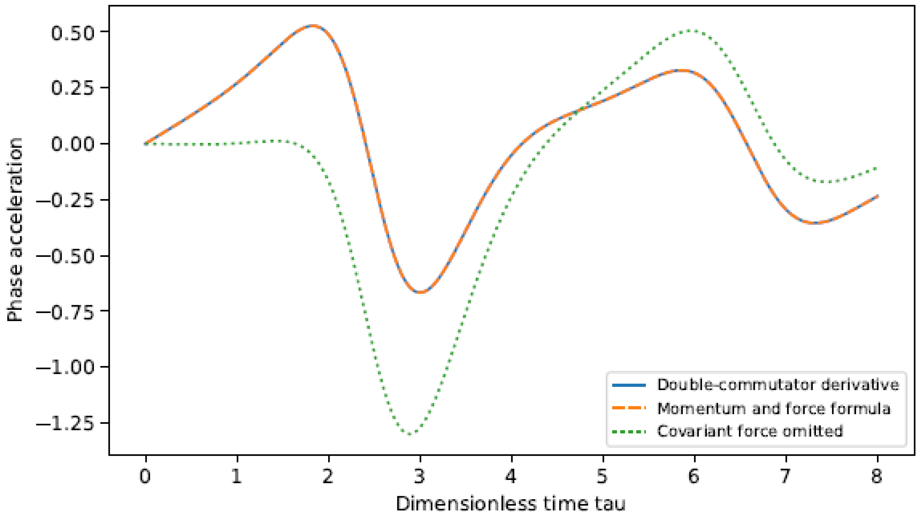
Table A1. Numerical comparisons from joint spectral evolution. All entries are model-generated, and phase derivatives use $\tau =t/T_R$.

Quantity	Maximum difference
Soluble coherence, spectral versus analytic	$9.01\times {10}^{-16}$
Soluble phase rate, spectral versus analytic	$5.00\times {10}^{-16}$
Soluble phase acceleration, spectral versus analytic	$4.10\times {10}^{-16}$
Physical coherence versus Eq. (43)	$7.45\times {10}^{-16}$
Reduced purity versus Eq. (44)	$7.78\times {10}^{-16}$
Coherence in the identical-marginal example	$2.24\times {10}^{-16}$
Noncommuting coherence, $N=8$ versus $N=12$	$1.59\times {10}^{-14}$
Noncommuting phase acceleration, two formulas	$1.06\times {10}^{-15}$
Noncommuting phase acceleration, force omitted	$7.71\times {10}^{-1}$

Table A1. Numerical comparisons from joint spectral evolution. All entries are model-generated, and phase derivatives use $\tau =t/T_R$.

Quantity	Maximum difference
Soluble coherence, spectral versus analytic	$9.01\times {10}^{-16}$
Soluble phase rate, spectral versus analytic	$5.00\times {10}^{-16}$
Soluble phase acceleration, spectral versus analytic	$4.10\times {10}^{-16}$
Physical coherence versus Eq. (43)	$7.45\times {10}^{-16}$
Reduced purity versus Eq. (44)	$7.78\times {10}^{-16}$
Coherence in the identical-marginal example	$2.24\times {10}^{-16}$
Noncommuting coherence, $N=8$ versus $N=12$	$1.59\times {10}^{-14}$
Noncommuting phase acceleration, two formulas	$1.06\times {10}^{-15}$
Noncommuting phase acceleration, force omitted	$7.71\times {10}^{-1}$

At the balanced-preparation zero, the phase is undefined. Direct spectral evaluation gives $|c\left(t_{*}\right)|=2.61\times {10}^{-16}$ and $Tr{\rho }_X{\left(t_{*}\right)}^2=0.5000000000000004$, consistent with the exact zero and purity $1/2$. The displayed residues are consistent with floating-point roundoff.

Appendix E.2 Correlation Flow and Joint-Record Probabilities

The script correlation_dynamics.py compares three calculations on the invariant support: spectral evolution of the full $4\times 4$ density operator, integration of the four complex moments, and integration of the scalar fourth-order equation in the carrier-rotating frame. An independently chosen positive mixed state tests all four moment directions. Symbolic Pauli algebra gives Eq. (61), the characteristic identity (65), and the determinant (67) exactly.

Figure A2. Four joint moments for a positive mixed preparation, with $\kappa =0.23$, ${\omega }_x{T}_R=0.9$, and ${\omega }_z{T}_R=0.7$. Their magnitudes vary while their squared-magnitude sum is conserved. The joint density evolution and the closed correlation system coincide.

Figure A2. Four joint moments for a positive mixed preparation, with $\kappa =0.23$, ${\omega }_x{T}_R=0.9$, and ${\omega }_z{T}_R=0.7$. Their magnitudes vary while their squared-magnitude sum is conserved. The joint density evolution and the closed correlation system coincide.

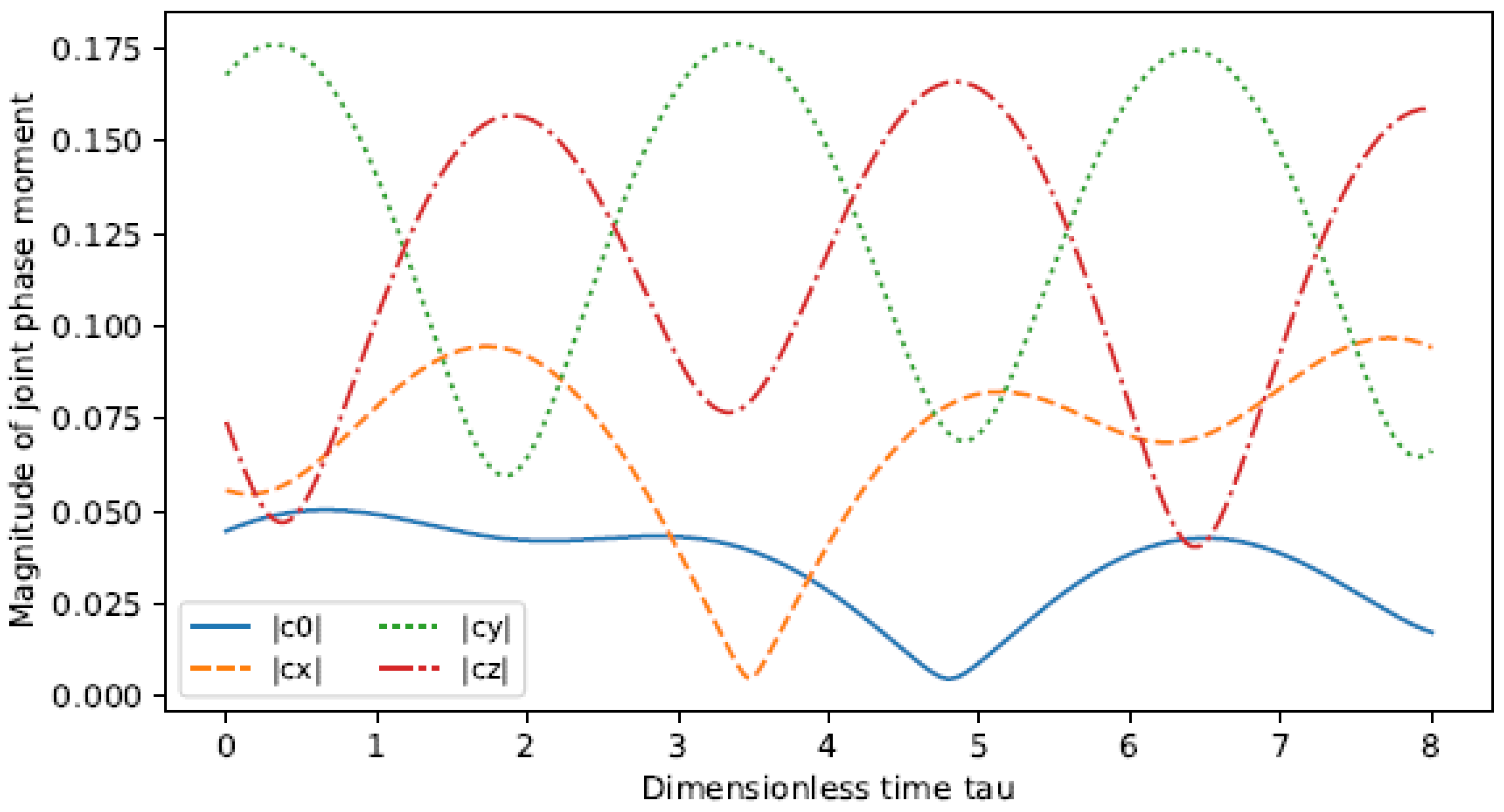
For $0\le \tau \le 8$ and 1601 common output times, the largest complex-moment difference between spectral evolution and the four-moment integration is $6.63\times {10}^{-14}$; the fourth-order scalar calculation differs from the spectral $c_0$ by at most $1.78\times {10}^{-14}$. The largest derivative discrepancy between the full commutator and the moment generator is $5.60\times {10}^{-17}$. For the paired preparations, both marginal differences and the drive-off coherence difference vanish at the reported precision. On $0\le \tau \le 5$, their readout amplitudes remain above $0.1702$, so the displayed phase comparison does not cross a first-moment zero.

Integrating the joint probabilities computed from the density operator reproduces the operator moments to $3.68\times {10}^{-16}$. For a rectangular window of width $0.6$ centered at $\tau =2.2$, quadrature of the joint solution and evaluation of $F_w\left(M\right)$ differ by at most $2.93\times {10}^{-16}$.

Appendix E.3 Projective Phase Dynamics and Continuation

For a nonzero-readout comparison, take the same parameters as in Section 7: $\gamma =0.23$, ${\omega }_x=0.9$, ${\overline{\omega }}_z=0.47$, and ${\omega }_c=0.5$ in $T_R$ units. Set the initial ratios to (81), with $c_0\left(0\right)=0.02$. The density operator (69) has minimum eigenvalue $0.1368931$. The interval $0\le \tau \le 3$ uses 1201 common output points.

The full joint density operator is propagated spectrally. Independent DOP853 integrations propagate the ratio flow and the normalized-derivative flow, each with its phase equation. Relative and absolute tolerances are $3\times {10}^{-13}$ and $2\times {10}^{-15}$; a second run uses $2\times {10}^{-11}$ and $2\times {10}^{-13}$. The minimum first-harmonic magnitude on the output grid is about $0.0200$. The tighter comparisons are summarized in Table A2.

Table A2. Independent representations of the quantum phase dynamics. Values are maximum absolute differences on the stated grids, with derivatives in dimensionless time.

Quantity	Maximum difference
Ratio state versus joint spectral evolution	$1.58\times {10}^{-12}$
Integrated phase versus joint spectral phase	$1.52\times {10}^{-13}$
Normalized-derivative state versus ratio representation	$3.78\times {10}^{-13}$
Reconstructed complex first harmonic versus joint state	$3.32\times {10}^{-15}$
Phase acceleration from Eq. (73) versus joint state	$6.90\times {10}^{-13}$
Phase increments after a common complex rescaling	$1.20\times {10}^{-15}$
Projective-chart reconstruction across a first-harmonic zero	$5.70\times {10}^{-14}$
Filtered first harmonic versus common-window reduced flow	$3.24\times {10}^{-15}$

Table A2. Independent representations of the quantum phase dynamics. Values are maximum absolute differences on the stated grids, with derivatives in dimensionless time.

Quantity	Maximum difference
Ratio state versus joint spectral evolution	$1.58\times {10}^{-12}$
Integrated phase versus joint spectral phase	$1.52\times {10}^{-13}$
Normalized-derivative state versus ratio representation	$3.78\times {10}^{-13}$
Reconstructed complex first harmonic versus joint state	$3.32\times {10}^{-15}$
Phase acceleration from Eq. (73) versus joint state	$6.90\times {10}^{-13}$
Phase increments after a common complex rescaling	$1.20\times {10}^{-15}$
Projective-chart reconstruction across a first-harmonic zero	$5.70\times {10}^{-14}$
Filtered first harmonic versus common-window reduced flow	$3.24\times {10}^{-15}$

Figure A3. Phase increments obtained from the joint density operator, correlation ratios, and normalized derivatives, using the same initial state and Hamiltonian. The known carrier is removed for display.

Figure A3. Phase increments obtained from the joint density operator, correlation ratios, and normalized derivatives, using the same initial state and Hamiltonian. The known carrier is removed for display.

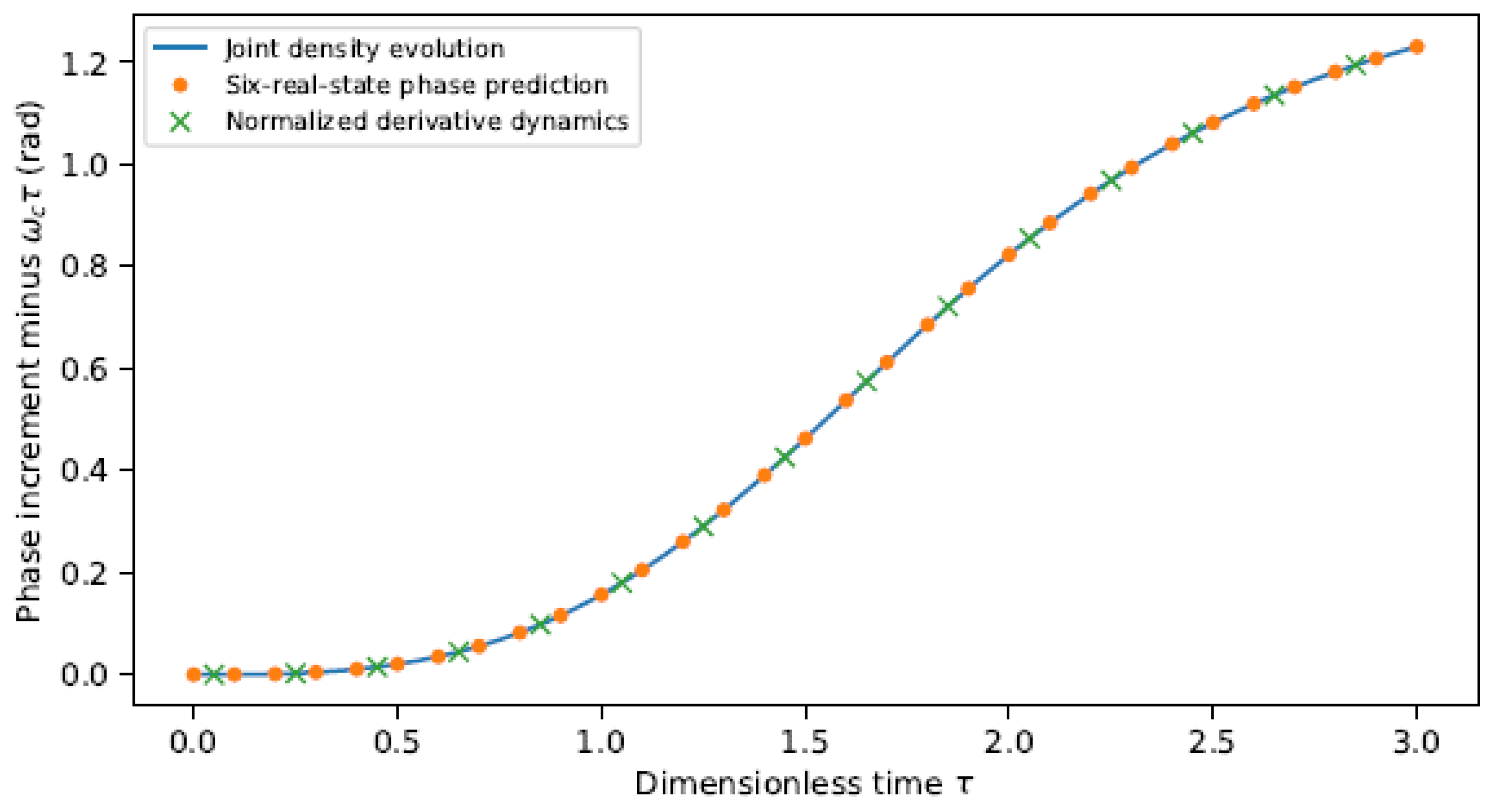
A second physical preparation multiplies the initial moment vector by $0.65e^{0.37\mathrm{i}}$. It changes the initial amplitude and phase while leaving the ratios unchanged. After subtracting the respective initial phase origins, the two unit phase-increment factors agree to $1.20\times {10}^{-15}$. The difference between the two integration tolerances is $1.10\times {10}^{-11}$ rad in the phase, consistent with convergence of the reduced calculations.

For the zero-crossing example (102), use $\gamma =0.23$, $\eta =0.1$, and $0\le \tau \le 12$. The first zero occurs at ${\tau }_{*}=6.8295492469$. A chart change from $c_0$ to $c_z$ occurs before this time; it is triggered when a competing coordinate ratio reaches modulus two. Spectral evolution gives $|c_0\left({\tau }_{*}\right)|<5\times {10}^{-17}$ and $|c_z\left({\tau }_{*}\right)|=0.1$ at numerical precision. No phase is reported at that time. The continued charts reconstruct the full complex moments with the error in Table A2.

Figure A4. Continuation through a zero of $c_0$. The nonzero component $c_z$ supplies a regular chart when the first-harmonic chart fails. Triangles mark chart changes; the dotted line marks the instant at which the measured phase is undefined.

Figure A4. Continuation through a zero of $c_0$. The nonzero component $c_z$ supplies a regular chart when the first-harmonic chart fails. Triangles mark chart changes; the dotted line marks the instant at which the measured phase is undefined.

Appendix E.4 Finite-Record Reconstruction and Withheld Prediction

The numerical example keeps the parameters and positive initial joint state used for the phase-reduction comparison:

$$(\gamma ,{\omega }_x,{\overline{\omega }}_z,{\omega }_c)=(0.23,0.9,0.47,0.5),c_0\left(0\right)=0.02,$$

with the ratios in (81). Times are in units $T_R$. The reference at $\tau =0$ and six phases at $\tau =2,4,6,8,10,12$ are computed from the full $4\times 4$ joint density operator. Only their unit factors, timestamps, and calibrated generator are supplied to (109). The initial density operator and the later records are withheld from the reconstruction. The recovered state then predicts the phase on $12<\tau \le 18$.

The phase matrix has smallest singular value $0.0244226$ and condition number $66.8948$. The recovered ratio state differs from the generating state by $1.90\times {10}^{-13}$ in Euclidean norm; the largest circular phase difference on the later grid is $2.11\times {10}^{-15}$ rad. A common initial scaling by $0.65e^{0.37\mathrm{i}}$ changes neither the ideal phase-increment data nor the inferred state, up to numerical roundoff.

Figure A5. Reconstruction and later phase prediction from one reference and six terminal estimates. The inverse routine receives the phase factors, times, and generator, while the initial joint state and later records are reserved for comparison. The vertical line marks the last reconstruction time. The carrier is removed for display.

Figure A5. Reconstruction and later phase prediction from one reference and six terminal estimates. The inverse routine receives the phase factors, times, and generator, while the initial joint state and later records are reserved for comparison. The vertical line marks the last reconstruction time. The carrier is removed for display.

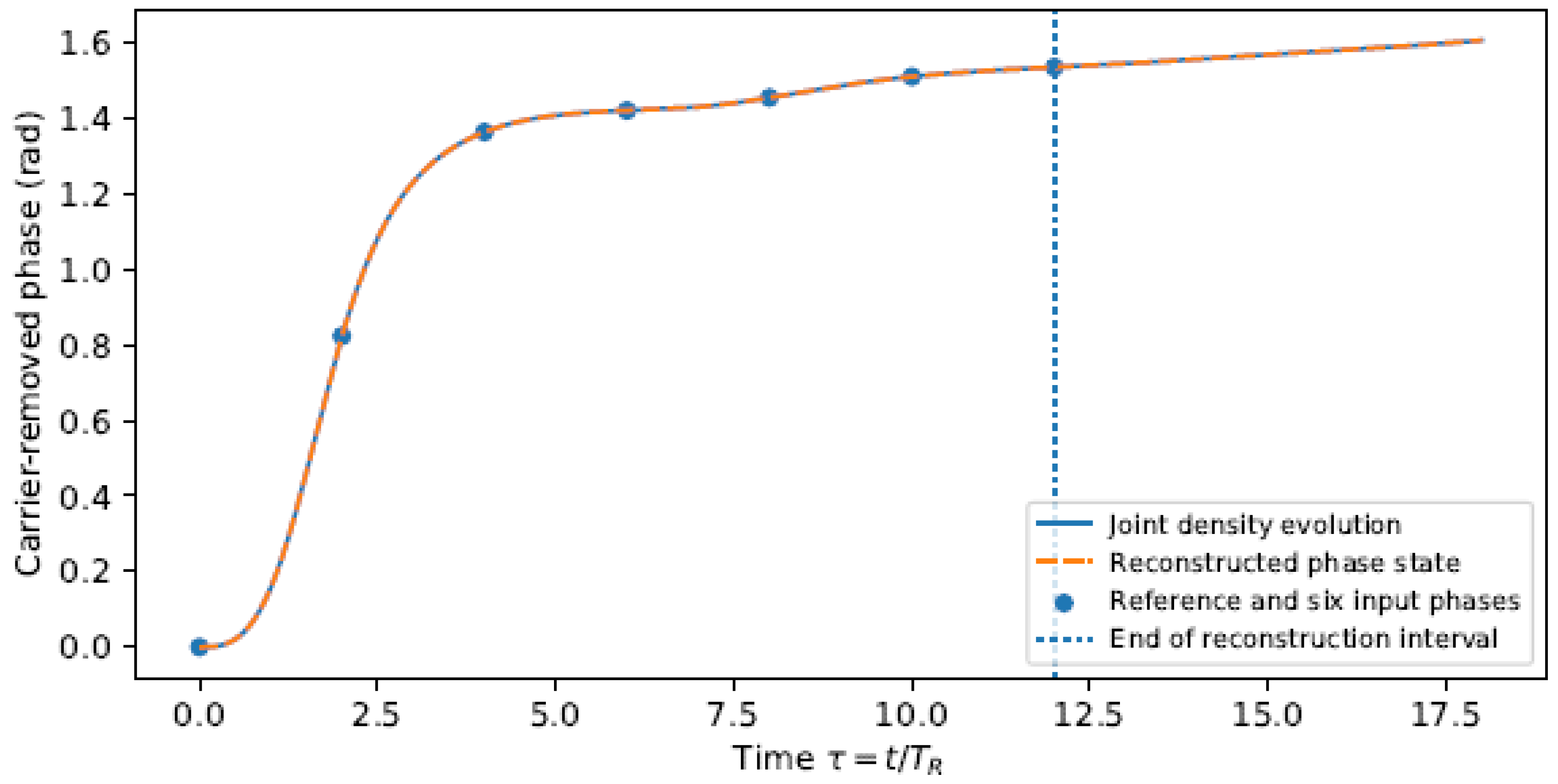
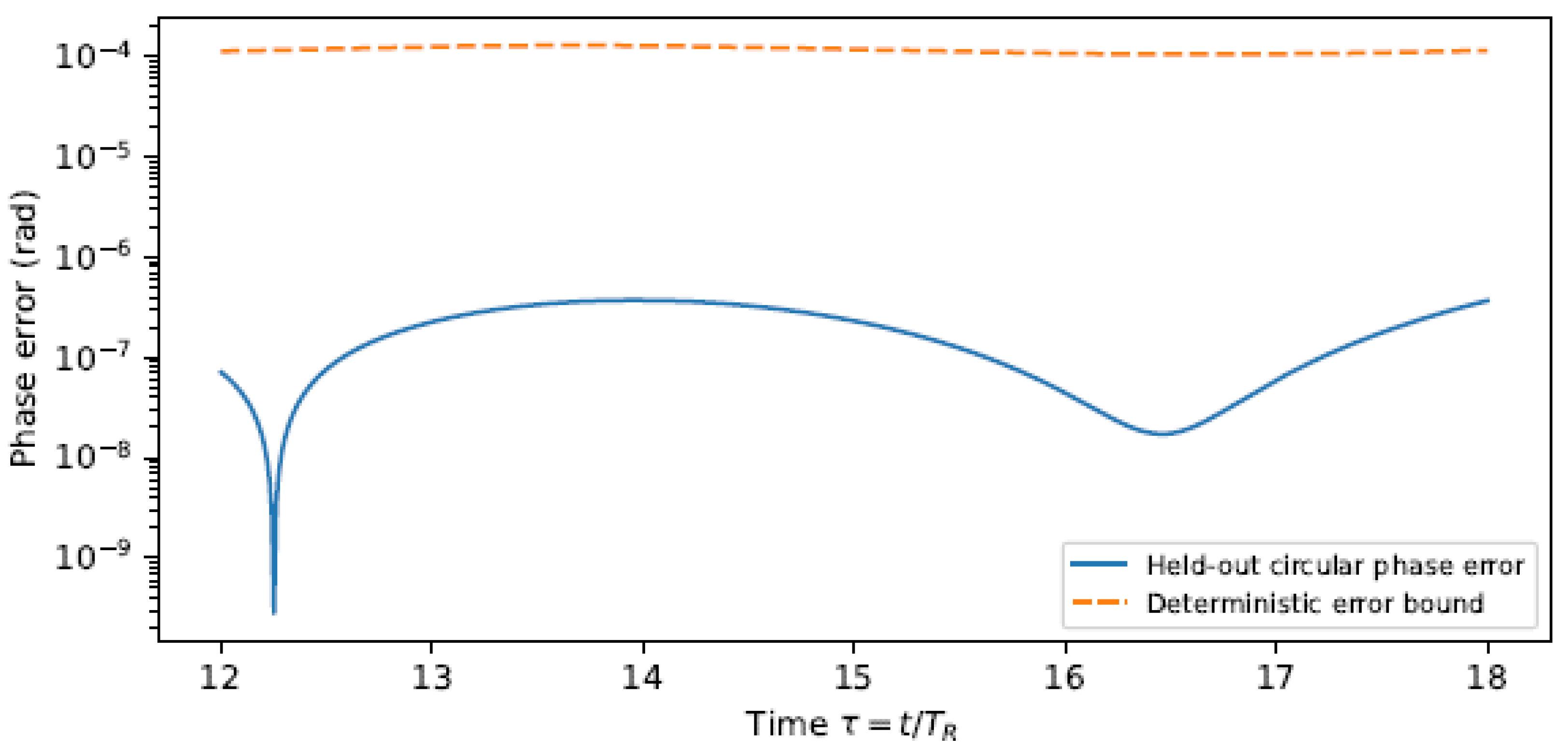
A second calculation adds bounded angular perturbations of at most $5\times {10}^{-7}$ rad to each absolute phase, including the shared reference. Thus each increment has error at most ${10}^{-6}$ rad. These prescribed errors test the sensitivity bound; they are not a detector noise model. The ratio-state error is $8.01\times {10}^{-5}$, below the a posteriori bound $1.04\times {10}^{-3}$. The largest later phase error is $3.71\times {10}^{-7}$ rad, while the largest bound in (116) is $1.28\times {10}^{-4}$ rad. On a grid of spacing $0.005$, Eq. (117) gives a positive normalized-readout margin of $0.9930$ throughout $0\le \tau \le 18$.

Figure A6. Later phase error and its deterministic bound for records with prescribed bounded perturbations. Every increment includes the shared reference error. The generator is held fixed throughout the reconstruction and prediction.

Figure A6. Later phase error and its deterministic bound for records with prescribed bounded perturbations. Every increment includes the shared reference error. The generator is held fixed throughout the reconstruction and prediction.

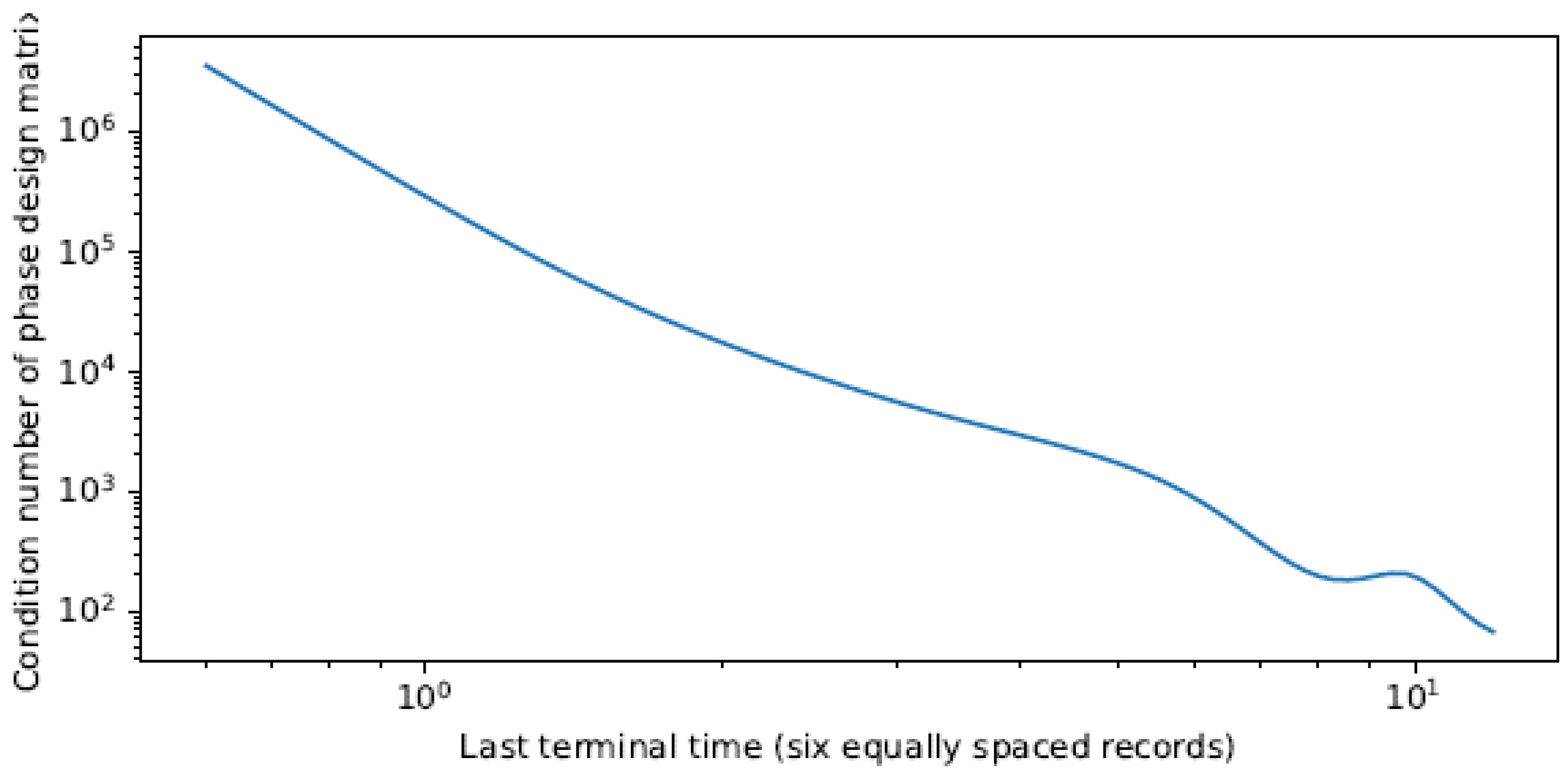
Compressing the same six-point schedule changes its condition number markedly. End times $\tau =1,3,6,12$ give values of approximately $2.83\times {10}^5$, $5.46\times {10}^3$, 864, and $66.9$. The trend applies to this state and these schedules; long intervals can also lose information through mode recurrences. For $r_x=r_z=0$ and $r_y=\mathrm{i}\gamma /{\omega }_x$, the normalized derivatives are real and the phase matrix has rank three. The inverse routine reports unresolved directions for this exceptional preparation.

Figure A7. Conditioning of the six-record inverse problem as the sampling interval is shortened. Distinct times preserve generic full rank, but the higher-order differences between phase histories become harder to resolve.

Figure A7. Conditioning of the six-record inverse problem as the sampling interval is shortened. Distinct times preserve generic full rank, but the higher-order differences between phase histories become harder to resolve.

The reconstructed phase is thus tested against later values from an independent propagation of the joint density operator. Experimental application requires the physical characterization described in Section 10.

References

- Meng, X. A set-theoretic derivation of Physobser axiom irreducibility, minimality, and essential uniqueness of the physical–observation dual-axis structure. Preprints 2026. [Google Scholar] [CrossRef]
- Meng, X. The phase transport fundamental equation on the physical–observation dual-axis structure. Preprints 2026. [Google Scholar] [CrossRef]
- Aharonov, Y.; Kaufherr, T. Quantum frames of reference. Phys. Rev. D. 1984, 30, 368–385. [Google Scholar] [CrossRef]
- Giacomini, F.; Castro-Ruiz, E.; Brukner, Č. Quantum mechanics and the covariance of physical laws in quantum reference frames. Nat. Commun. 2019, 10, 494. [Google Scholar] [CrossRef] [PubMed]
- Pancharatnam, S. Generalized theory of interference, and its applications. Part I. Coherent pencils. Proc. Indian Acad. Sci. A 1956, 44, 247–262. [Google Scholar] [CrossRef]
- Kato, T. On the adiabatic theorem of quantum mechanics. J. Phys. Soc. Jpn. 1950, 5, 435–439. [Google Scholar] [CrossRef]
- Berry, M. V. Quantal phase factors accompanying adiabatic changes. Proc. R. Soc. Lond. A 1984, 392, 45–57. [Google Scholar] [CrossRef]
- Simon, B. Holonomy, the quantum adiabatic theorem, and Berry’s phase. Phys. Rev. Lett. 1983, 51, 2167–2170. [Google Scholar] [CrossRef]
- Aharonov, Y.; Anandan, J. Phase change during a cyclic quantum evolution. Phys. Rev. Lett. 1987, 58, 1593–1596. [Google Scholar] [CrossRef] [PubMed]
- Heslot, A. Quantum mechanics as a classical theory. Phys. Rev. D. 1985, 31, 1341–1348. [Google Scholar] [CrossRef] [PubMed]
- Susskind, L.; Glogower, J. Quantum mechanical phase and time operator. Phys. Phys. Fiz. 1964, 1, 49–61. [Google Scholar] [CrossRef]
- Lévy-Leblond, J.-M. Who is afraid of nonhermitian operators? A quantum description of angle and phase. Ann. Phys. 1976, 101, 319–341. [Google Scholar] [CrossRef]
- Robertson, H. P. The uncertainty principle. Phys. Rev. 1929, 34, 163–164. [Google Scholar] [CrossRef]
- Pechukas, P. Reduced dynamics need not be completely positive. Phys. Rev. Lett. 1994, 73, 1060–1062. [Google Scholar] [CrossRef] [PubMed]
- Hermann, R.; Krener, A. J. Nonlinear controllability and observability. IEEE Trans. Autom. Control 1977, 22(5), 728–740. [Google Scholar] [CrossRef]
- Sussmann, H. J. Existence and uniqueness of minimal realizations of nonlinear systems. Math. Syst. Theory 1976, 10, 263–284. [Google Scholar] [CrossRef]
- Sjöqvist, E.; Pati, A. K.; Ekert, A.; Anandan, J. S.; Ericsson, M.; Oi, D. K. L.; Vedral, V. Geometric phases for mixed states in interferometry. Phys. Rev. Lett. 2000, 85, 2845–2849. [Google Scholar] [CrossRef] [PubMed]
- Aharonov, Y.; Albert, D. Z.; Vaidman, L. How the result of a measurement of a component of the spin of a spin-1/2 particle can turn out to be 100. Phys. Rev. Lett. 1988, 60, 1351–1354. [Google Scholar] [CrossRef] [PubMed]
Figure 4.
Phase response to opposite initial correlations. The preparations in Eq. (83) have equal marginals, coherence, and initial phase rate. A transverse generator gives opposite accelerations; with that generator absent, the histories coincide. Parameters are given in Eq. (89), and the common carrier is removed in the display.
Disclaimer/Publisher’s Note: The statements, opinions and data contained in all publications are solely those of the individual author(s) and contributor(s) and not of MDPI and/or the editor(s). MDPI and/or the editor(s) disclaim responsibility for any injury to people or property resulting from any ideas, methods, instructions or products referred to in the content. |
© 2026 by the authors. Licensee MDPI, Basel, Switzerland. This article is an open access article distributed under the terms and conditions of the Creative Commons Attribution (CC BY) license (http://creativecommons.org/licenses/by/4.0/).
Copyright: This open access article is published under a Creative Commons CC BY 4.0 license, which permit the free download, distribution, and reuse, provided that the author and preprint are cited in any reuse.