The Enigma of the Planck Resonator Solved: It Is a Physical Wave Window

1. Introduction

One presents here an original and unpublished derivation of Planck’s law from the Stefan-Boltzmann law combined with dimensional analysis [1], without resorting to the usual Rayleigh-Jeans law. The Stefan-Boltzmann law gives the black body radiance of physical dimension “W⋅L^-2.” However, performing a dimensional analysis on the result of applying Wien’s displacement law to the Stefan-Boltzmann law, one notices the element “1/λ²” of physical dimension “L^-2.” Indeed, “λ²” is a square surface with side “λ,” and whose inverse “1/λ²” is its number N per unit area. One names this element a “Wave window,” by analogy with a window that lets radiation pass in both directions according to Kirchhoff’s law of thermal radiation. So, one has a formula where the unit area energy flux is equal to N times the energy flux radiated by a Wave window. Then, one only has to consider statistically the energy radiated by Wave windows in a unit area per unit time on the model of the kinetic energy of perfect gas molecules in a mole, all at thermal equilibrium.

Thus, in pursuing the quest for the distribution of energy in the blackbody radiation formula initiated by Gustav Kirchhoff in 1860 [2,3], Max Planck leaves the framework of experimentation in wavelength and radiation power per unit area for an equivalent framework in frequency and energy density of radiation. He then found himself in a theoretical environment close to that used by Maxwell and Boltzmann for the statistical calculation of a perfect gas. Thus, he would be able to find a demonstration justifying his empirical adaptation correcting the failure of the Wilhelm Wien distribution for long wavelengths, by simply adding the operation “-1” to the denominator [4]:

$$E={\displaystyle \frac{C{\lambda }^{-5}}{e^{\frac{c}{\lambda T}}-1}}$$

(1)

Afterwards, by considering an energy composed of finite equal parts and inspired by Boltzmann’s combinatorial-probabilistic treatment of perfect gases, linked to entropy, he provides a demonstration which leads to this result [3,5,6,7].

However, introducing the Wave window energy produces this new formula:

$$E={\lambda }^{-2}\cdot {\displaystyle \frac{C{\lambda }^{-3}}{e^{\frac{c}{\lambda T}}-1}}$$

This gives the average Wave windows energy:

$$E_w={\displaystyle \frac{C{\lambda }^{-3}}{e^{\frac{c}{\lambda T}}-1}}$$

One then finds the first equation from Planck’s article in 1901: “E=N ∙E_w.” One can therefore simply use the Wave window, a physical object traversed by an energy comparable to the kinetic energy of a gas molecule (see Debye [8,9]), to replace the hypothetical Planck resonator, and take up an original derivation of Planck’s law from the Stefan-Boltzmann law.

2. Demonstration

2.1. The Framework

In this experimental framework, one measures the radiant power per unit area and per steradian (radiance) for bandwidth segments of the total radiant power. In fact, the measuring element of a spectroradiometer, such as a bolometer or a photodiode, with or without a bandpass filter, gives the same arbitrary quantity of radiance. Thus, if the bandwidth of this spectroradiometer is scaled to 10^-9 m (a nanometer) using a simple rule of three, the same arithmetic value is obtained in radiance as in spectral radiance, using the trick of converting one dimension in meters to nanometers. Indeed, if one performs a spectral decomposition of the radiance by summing bandwidth segments, one adds two physical dimensions to them, those of wavelength (or frequency) and bandwidth, into a dimensionless function, and one uses it in the next chapter. Thus, staying within this framework simplifies the problem; it is unnecessary to consider the energy density, but only the energy flux through a surface: a power. So, one defines the basics of the naming convention in the following table:

Table 1. Above all, one has a remarkable point:.

λ	Mean wavelength in a bandwidth or wavelength group, with dimension “L” and SI unit “m,” separating a group of photons into two subgroups of equal energy.
Δλ	Wavelength interval or bandwidth of a spectroradiometer, with dimension “L” and SI unit “m.”
ν	Mean frequency in a bandwidth or frequency group, with dimension “T-1” and SI unit “Hz” (cycles/second), related to wavelength by ν=c/λ.
Δν	Frequency bandwidth, with dimension “T-1” and SI unit “Hz” (cycles/second).
c	Speed of light, with dimension “LT-1” and SI unit “m/s.”
T	Temperature, with dimension “θ” and SI unit “K.”
B(T)	Blackbody radiance for the entire spectrum (with SI unit “W⋅m−2sr−1”).
$B_{\lambda }(\lambda ,T)$	Planck’s law spectral radiance as a function of wavelength, for a given temperature (with SI unit “W⋅m−3sr−1”).
$B_{\lambda }(\lambda ,T,\Delta \lambda )$	Blackbody radiance as a function of wavelength, for a given temperature, and bandwidth (with arbitrary unit “W⋅m−2⋅sr−1”).
EN	Blackbody energy radiated per unit area, per unit of time, for a given wavelength and bandwidth (with SI unit “J”).
$B_{{\lambda }_w}(\lambda ,T,\Delta \lambda )$	Average blackbody radiance through a Wave window as a function of wavelength, for a given temperature, and bandwidth (with arbitrary unit “W⋅sr−1”).
Ew	Average blackbody energy radiated by a Wave Window, per unit of time, for a given wavelength and bandwidth (with SI unit “J”).
ε	Average elementary energy of blackbody radiation, distributed in equal parts, for a given wavelength. Now called “photon” (with SI unit “J”).

Table 1. Above all, one has a remarkable point:.

λ	Mean wavelength in a bandwidth or wavelength group, with dimension “L” and SI unit “m,” separating a group of photons into two subgroups of equal energy.
Δλ	Wavelength interval or bandwidth of a spectroradiometer, with dimension “L” and SI unit “m.”
ν	Mean frequency in a bandwidth or frequency group, with dimension “T-1” and SI unit “Hz” (cycles/second), related to wavelength by ν=c/λ.
Δν	Frequency bandwidth, with dimension “T-1” and SI unit “Hz” (cycles/second).
c	Speed of light, with dimension “LT-1” and SI unit “m/s.”
T	Temperature, with dimension “θ” and SI unit “K.”
B(T)	Blackbody radiance for the entire spectrum (with SI unit “W⋅m−2sr−1”).
$B_{\lambda }(\lambda ,T)$	Planck’s law spectral radiance as a function of wavelength, for a given temperature (with SI unit “W⋅m−3sr−1”).
$B_{\lambda }(\lambda ,T,\Delta \lambda )$	Blackbody radiance as a function of wavelength, for a given temperature, and bandwidth (with arbitrary unit “W⋅m−2⋅sr−1”).
EN	Blackbody energy radiated per unit area, per unit of time, for a given wavelength and bandwidth (with SI unit “J”).
$B_{{\lambda }_w}(\lambda ,T,\Delta \lambda )$	Average blackbody radiance through a Wave window as a function of wavelength, for a given temperature, and bandwidth (with arbitrary unit “W⋅sr−1”).
Ew	Average blackbody energy radiated by a Wave Window, per unit of time, for a given wavelength and bandwidth (with SI unit “J”).
ε	Average elementary energy of blackbody radiation, distributed in equal parts, for a given wavelength. Now called “photon” (with SI unit “J”).

Since the area of a Wave window is equal to λ², the number N of Wave windows per unit area is simply ⌊1/λ²⌋.

2.2. Stefan-Boltzmann’s Law

To highlight the Wave window in the demonstration of Planck’s law, one starts with its relation to the Stefan-Boltzmann law [11]. It states that the black body’s radiance is proportional to the fourth power of its temperature [3,4]:

$$B\left(T\right)={\displaystyle \frac{\sigma }{\pi }}{T}^4$$

(2)

However, in experimentation, infinitesimal bandwidths and power are excluded, with the minimal power of a photon’s energy per unit of time. Therefore, taking the simplest approximate discrete integral, a middle Riemann sum bounded by the wavelengths λ1 and λ2 covering the entire blackbody radiation spectrum, for the radiation spectrum by wavelength λ, bandwidth Δλ, and by bandwidth step Δλ that gives:

$$n={\displaystyle \frac{{\lambda }_2-{\lambda }_1}{\Delta \lambda }},{\lambda }_2>{\lambda }_1$$

$${\lambda }_i={\lambda }_1+i\cdot \Delta \lambda -{\displaystyle \frac{\Delta \lambda }{2}}={\lambda }_1+(i-{\displaystyle \frac{1}{2}})\cdot \Delta \lambda$$

$$B\left(T\right)={\sum }_{i=0}^{n}B({\lambda }_i,T)\cdot \Delta \lambda$$

(3)

Furthermore, remaining in the same physical dimension of power per square meter, by combining equations (2) and (3), one obtains:

$$B\left(T\right)={\sum }_{i=0}^n{\displaystyle \frac{\sigma }{\pi }}{T}^4\cdot f_1({\lambda }_i,T)\cdot \Delta \lambda$$

(4)

Moreover, one notices from (2), (3), and (4) that the element “$f_1({\lambda }_i,T)\cdot \Delta \lambda$” is indeed dimensionless, and its sum is equal to one:

$$\sum _{i=0}^n{f}_1({\lambda }_i,T)\cdot \Delta \lambda =1$$

Then, to add the wavelength dimension, this dimensionless element “$f_1({\lambda }_i,T)\cdot \Delta \lambda$” can be divided again into two dimensionless members, “$f_2({\lambda }_i,T)$” and “${\displaystyle \frac{1}{{\lambda }_i}}\cdot \Delta \lambda$”:

$$B\left(T\right)={\sum }_{i=0}^n{\displaystyle \frac{\sigma }{\pi }}{T}^4\cdot f_2({\lambda }_i,T)\cdot {\displaystyle \frac{1}{{\lambda }_i}}\cdot \Delta \lambda$$

(5)

In addition, one can use another new function to get closer to the desired result:

$$B\left(T\right)={\sum }_{i=0}^n{{\displaystyle \frac{\sigma }{\pi }}T}^4\cdot {\displaystyle \frac{1}{f_3({\lambda }_i,T)}}\cdot {\displaystyle \frac{1}{{\lambda }_i}}\cdot \Delta \lambda$$

(6)

Ultimately, one remains within the same framework.

2.3. Wien’s Displacement Law

Wien’s displacement law states that the wavelength of maximum black-body radiation is inversely proportional to its temperature [3,12]. This gives the following formula: λ_peak⋅T=b, which one can therefore apply to the Stefan-Boltzmann law. So, from (6), one can leave the sum, and, for a peak wavelength λ and bandwidth Δλ, one obtains the spectral blackbody radiance:

$$B_{\lambda }(\lambda ,T,\Delta \lambda )={\displaystyle \frac{\sigma }{\pi }}\cdot {\displaystyle \frac{1}{{\lambda }^4}}{\cdot b}^4\cdot {\displaystyle \frac{1}{f_3(\lambda ,T)}}\cdot {\displaystyle \frac{1}{\lambda }}\cdot \Delta \lambda$$

(7)

One then finds the average spectral blackbody radiance of a Wave window by dividing by N:

$$B_{{\lambda }_w}(\lambda ,T,\Delta \lambda )={\displaystyle \frac{\sigma }{\pi }}\cdot {\displaystyle \frac{1}{{\lambda }^3}}{\cdot b}^4\cdot {\displaystyle \frac{1}{f_3(\lambda ,T)}}\cdot \Delta \lambda$$

(8)

Next, the wavelength is temporarily converted into frequency, which does not vary depending on the diathermal medium. So one replaces Δλ/λ with Δν/ν (approximately from (λ+Δλ)(ν-Δν)=c) and λ with c/ν. This gives:

$$B_{{\lambda }_w}(\lambda ,T,\Delta \lambda )={\displaystyle \frac{\sigma }{\pi }}{\cdot {\displaystyle \frac{1}{c^2}}\cdot b}^4\cdot \nu \cdot {\displaystyle \frac{1}{f_3(\lambda ,T)}}\cdot \Delta \nu$$

(9)

To generalize outside λ_peak, one simplifies all constants with a constant h and a new function. Thus, one obtains the Wave window average power, with its elementary energy “hν” multiplied by its number per unit of time:

$$B_{{\lambda }_w}(\lambda ,T,\Delta \lambda )=h\nu \cdot {\displaystyle \frac{1}{f_4(\lambda ,T)}}\cdot \Delta \nu$$

(10)

Indeed, the function f₄ is dimensionless, and Δν has the dimension T^-1, so only “hν” can have the dimension of energy.

2.4. Entropy of a Wave Window as a Function of its Energy Flux

Then, as the interaction between the radiation energy and the internal kinetic energy of atoms creates the entropy disorder in the walls of the blackbody cavity, this becomes comparable to the thermodynamic model of perfect gas molecules. Thus, for a given bandwidth, one can compare a Wave window and its energy flux per unit of time to a molecule and its kinetic energy. Indeed, the power radiated by all Wave windows, according to the Stefan-Boltzmann law, is proportional to the temperature, just like the kinetic energy of perfect gas molecules. So, one resumes Planck’s combinatorial demonstration in detail, with real Wave windows instead of hypothetical resonators. Furthermore, one knows the number N of Wave windows per unit area: ⌊1/λ²⌋.

Therefore, in one direction, one polarization, and a given mean wavelength, per unit of time, the correspondence between a system with the total energy E_N radiated per unit area, and the average energy E_w radiated by a Wave window is given by the formula:

$$E_N=N\cdot E_w$$

(11)

Furthermore, one considers the energy E_N as a discrete quantity of an integer number of finite equal parts, which one names ε. Then, it suffices to specify that a number P of ε is radiated per unit area with the following formula:

$$E_N=P\cdot \epsilon$$

(12)

Therefore, with the well-known but detailed combinatorial demonstration in Appendix A, one obtains with (28) the average energy of a Wave window:

$$E_w=\epsilon \cdot {\displaystyle \frac{1}{e^{\frac{\epsilon }{kT}}-1}}$$

(13)

Of course, with Kirchhoff’s thermal law, it is also the radiation energy absorbed by a Wave window in the same unit of time.

2.5. The Black Body Distribution Law

One can now express the black body distribution law. Thus, from (10) and (13), one deduces the formulas for the elementary energy ε and the function f_4:

$$\epsilon =h\nu$$

(14)

$${\displaystyle \frac{1}{f_4(\lambda ,T)}}={\displaystyle \frac{1}{e^{\frac{\epsilon }{kT}}-1}}$$

(15)

Next, given the double polarization of the radiation, one must consider the energy of 2N Wave windows per unit area [13,14,15]. Therefore, expanding from (10),(14) and (15), one obtains:

$$B_{\lambda }(\lambda ,T,\Delta \lambda )=2\cdot {\displaystyle \frac{1}{{\lambda }^2}}\cdot h{\displaystyle \frac{c}{\lambda }}\cdot {\displaystyle \frac{c}{{\lambda }^2}}\cdot {\displaystyle \frac{1}{e^{\frac{hc}{\lambda kT}}-1}}\cdot \Delta \lambda$$

$$B_{\lambda }(\lambda ,T,\Delta \lambda )=2\cdot {\displaystyle \frac{{hc}^2}{{\lambda }^5}}\cdot {\displaystyle \frac{1}{e^{\frac{hc}{\lambda kT}}-1}}\cdot \Delta \lambda$$

(16)

Thus, with this formula (16), one recovers a version of Planck’s law that includes the bandwidth. Furthermore, one finds the same SI units as in the Stefan-Boltzmann law: “W⋅sr⁻¹⋅m⁻²,” that is, the radiance measured by a spectroradiometer. Then, by dividing by Δλ, one recovers Planck’s law in terms of wavelength for an idealized monochromatic radiation:

$$B_{\lambda }(\lambda ,T)=2\cdot {\displaystyle \frac{{hc}^2}{{\lambda }^5}}\cdot {\displaystyle \frac{1}{e^{\frac{hc}{\lambda kT}}-1}}$$

(17)

One has therefore validated the replacement of the resonator by partitioning a unit surface area of the black body into Wave windows, traversed by an energy statistically comparable to that of a perfect gas molecule. However, bandwidth-free radiation does not exist in nature. It therefore seems to me that formula (16), updating the law to account for bandwidth, is more representative of the blackbody distribution in experiment, and this is explored further in the discussion that follows.

3. Discussion

One can compare the Wave window and the resonator to the “My Wife and My Mother-in-Law” illusion [16]. This is how Planck and scientists, influenced by the discoveries of Maxwell and Hertz’s radio waves, see only the resonator [17]. To escape this illusion, one must therefore change the paradigm to align with experimentation and begin with a physical dimension analysis of the law. One then notices the surface of a Wave window in the expression “1/λ².” Indeed, it corresponds to the physical dimension of the area in Planck’s law. Furthermore, this is not the only surprising point, as is the absence of the bandwidth parameter Δλ in Planck’s law, whereas in nature, this is impossible. Moreover, the version of the law that includes bandwidth gives the same power curves in wavelength and frequency; indeed, before and after Planck, continuous curves were always used, whereas with quantization, discrete curves should have been used. These two topics are further developed in the following chapters.

3.1. The Missing Bandwidth

When using formula (16), one can predict the result of a spectroradiometer with a given bandwidth, whereas, implicitly, Planck’s law does not. Furthermore, the energy quantum contradicts Planck’s assumption of “dλ” as an infinitesimal bandwidth, and especially if the bandwidth tends towards zero, i.e., towards a monochromatic radiation, the power of the radiation also tends towards zero. This energy quantum per unit time defines the minimum bandwidth that one can obtain from (16):

$$\Delta {\lambda }_{min}=(e^{{\displaystyle \frac{hc}{\lambda kT}}}-1)\cdot {\displaystyle \frac{{\lambda }^4}{2c}}$$

(18)

Thus, statistically, each photon energy quantum has its own bandwidth, as in the following figure:

Figure 1. Zoom in on adjacent Wave windows.

Figure 1. Zoom in on adjacent Wave windows.

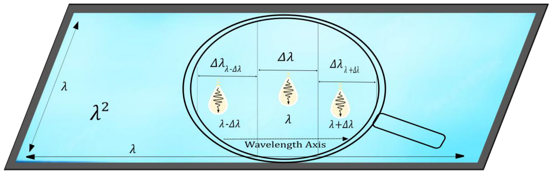
Nevertheless, Planck’s concept of monochromatic radiation can be updated by considering it as a group of photons within a given bandwidth Δλ and represented by their mean wavelength λ, separating two subgroups of equal energy. This is what one finds approximately in spectroradiometers and in formula (16).

3.2. An Intuitive Curve Based on Experimentation

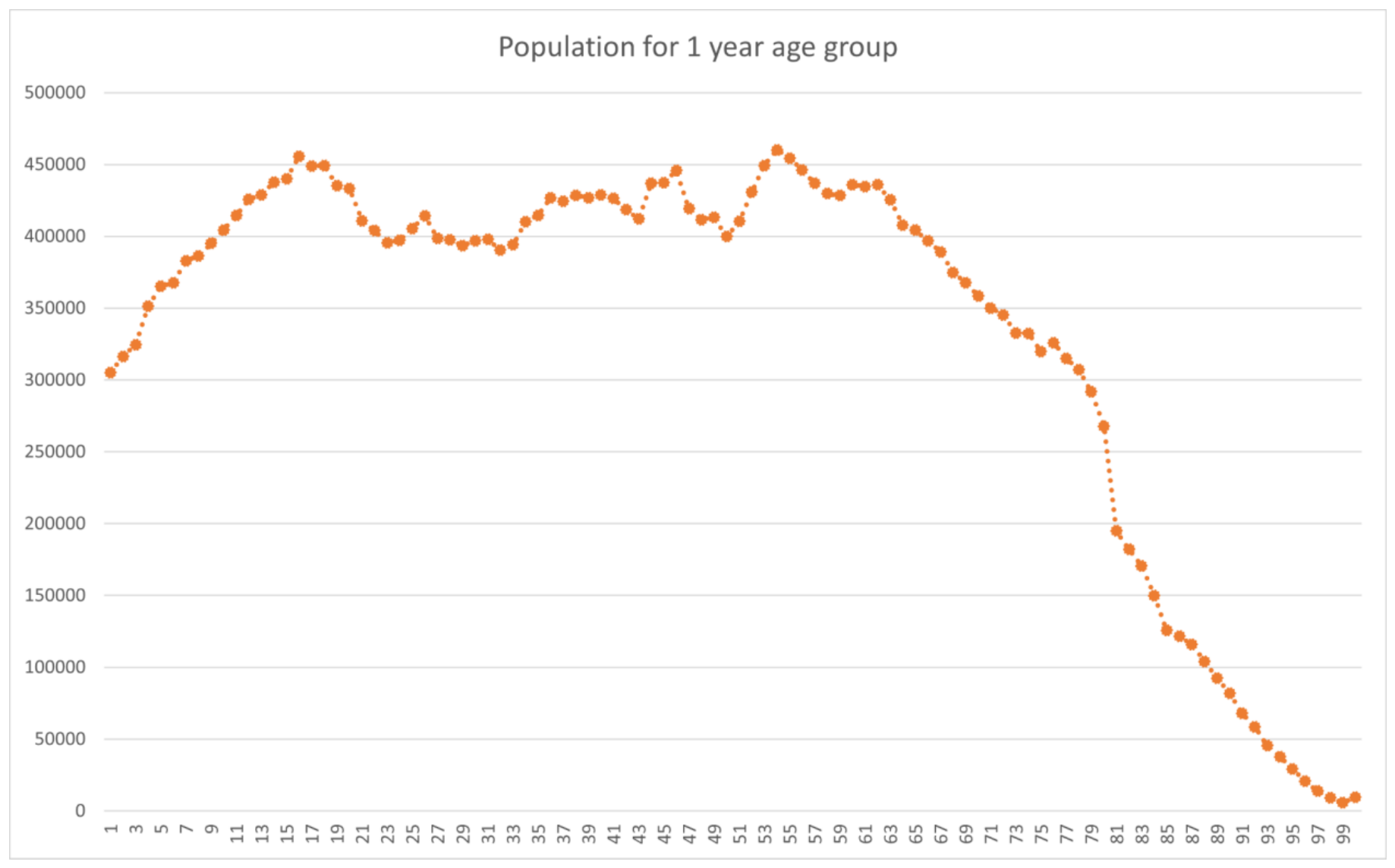
With formula (16), the result of a spectroradiometer with a given bandwidth can give the same power curve in wavelength as in frequency, whereas Planck’s law does not, leading to educational confusion [18]. However, since the power is quantized for a mean wavelength in its bandwidth, the wavelengths are also quantized, and if one takes their corresponding frequency and bandwidth values, one obtains the same maxima in the curves. This yields a dotted line curve, following the same principle as a population histogram by age group [19], with the mean wavelengths and frequencies as abscissa and radiance as ordinate. Furthermore, the peculiarity of this discrete curve is that the sum of the ordinates of each group corresponds to the total of all group elements.

To illustrate this, one presents a table of similarities and the type of graph:

Black-body radiation curve	Population pyramid
Wavelength or frequency	Age
Mean wavelength or frequency in its bandwidth, or wavelength group or frequency group	Age group
Radiance	Population

Black-body radiation curve	Population pyramid
Wavelength or frequency	Age
Mean wavelength or frequency in its bandwidth, or wavelength group or frequency group	Age group
Radiance	Population

Figure 2.

Figure 2.

Then, one can take the following black body experiment example:

• The temperature is measured with several sensors to guarantee its stability and uniformity.
• Radiation power is measured in radiance with a spectroradiometer behind a standard bandpass filter.
• One considers a standard bandpass filter with an FWHM of 1 nm, which one assigns to Δλ.
• One set the temperature to 3000K.

With these parameters, one simulates measurements using formula (16), reported in Table 3:

Therefore, one sees a single curve where the maximum wavelength value corresponds to its equivalent frequency $\nu \left(\lambda \right)={\displaystyle \frac{c}{\lambda }}$. The temperature and Δλ are constant parameters for each curve with a variable function $\Delta \nu \left(\lambda \right)={\displaystyle \frac{c}{{\lambda }^2}}\cdot \Delta \lambda$. They appear neither on the ordinate nor the abscissa.

Figure 3. dvsf.

Figure 3. dvsf.

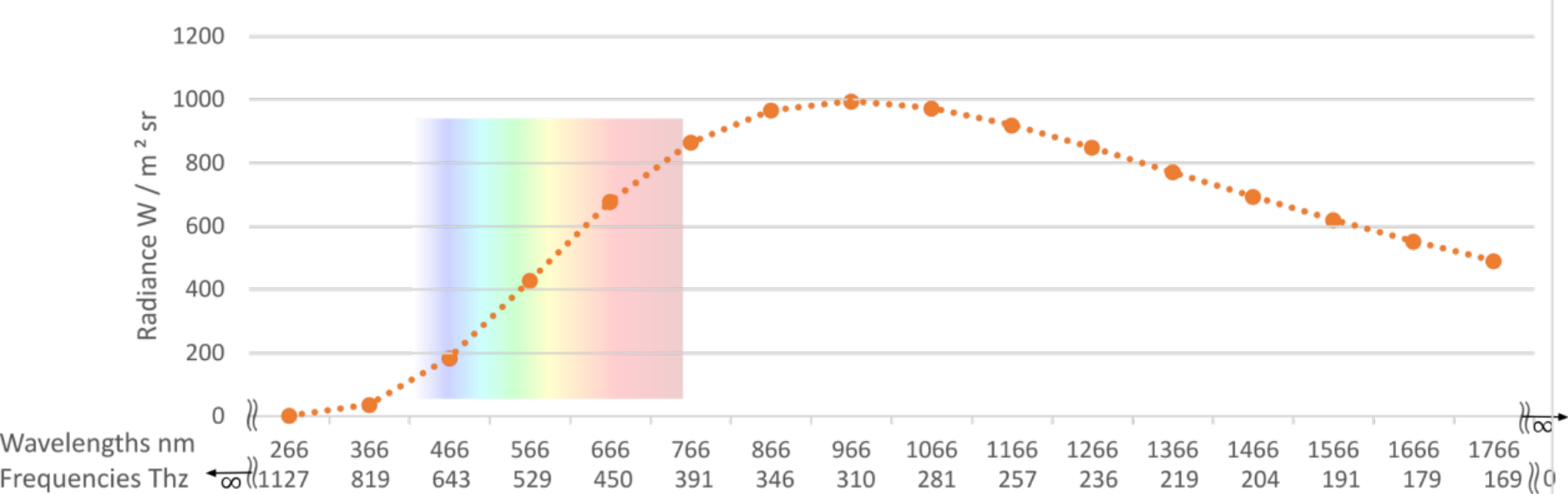
So, in this chapter, one has shown a more pedagogical approach to presenting the different curves of Planck’s law in physics and astronomy courses.

4. Conclusion and Outlook

By revisiting the demonstration of Planck’s law through dimensional analysis, one reveals the physical element hidden behind the resonator: the Wave window, a square whose side is equal to the wavelength. However, to validate it, a paradigm shift is necessary. In this new paradigm, one remains in the experimental context of measuring the power of radiation passing through the surface of the black body cavity wall. For entropy, one notes an equivalence for the energy passing through this Wave window per unit of time, the kinetic energy of a perfect gas molecule, and that of a resonator. Therefore, the Wave window can be used to reproduce Max Planck’s combinatorial demonstration. Next, the Wave window is special: it is a passive object for radiation, while the resonator is an active object, similar to a dipole antenna. This difference is fundamental: it brings one back to the field of geometric optics, which is more in line with Maxwell’s electromagnetism and Boltzmann’s statistics. Moreover, by assuming the quantization of energy, one uses a discrete Riemann sum rather than a definite integral, which highlights the bandwidth as a crucial parameter of the blackbody radiation distribution law. This updates Planck’s law in a form that allows for predicting spectroradiometer measurements implicitly and producing identical discrete power curves in wavelength and frequency for the same bandwidth.

Furthermore, the Wave window introduces a new hypothesis. Radiation energy enters and circulates disorderly in matter as entropy, agitates the atoms as temperature, and finally exits. That summarizes Kirchhoff’s thermal law and the three laws of thermodynamics.

Thus, the discovery of the Wave window opens the way to a revision of concepts that, at first glance, seem counterintuitive in quantum physics. The next one is the notion of wave-particle duality of electromagnetic radiation, where one will focus on demonstrating and experimenting, through radio waves, that one does indeed have a flux of photons/particles whose intensity is modulated over time in the same way as the electric current of an antenna.

References

- Williams, Jeffrey H. Dimensional Analysis: The great principle of similitude; IOP Publishing: Bristol, UK, 2021. [Google Scholar] [CrossRef]
- Kirchhoff, G. Ueber das Verhältniss zwischen dem Emissionsvermögen und dem Absorptionsvermögen der Körper für Wärme und Licht. Ann. Der Phys. 1860, Vol. 185(Issue 2), 275–301. [Google Scholar] [CrossRef]
- Mavani, H.; Singh, N. A Concise History of the Black-body Radiation Problem. Reson 2024, 29, 645–670. [Google Scholar] [CrossRef]
- Planck, M. Ueber eine Verbesserung der Wien’schen Spectralgleichung. Verhandlungen Der Dtsch. Phys. Ges. Im. Jahre 1900, 2, 202–204. [Google Scholar]
- Planck, M. Ueber das Gesetz der Energieverteilung im Normalspectrum. Ann. Der Phys. 1901, vol.309(Issue 3), 553–563. [Google Scholar] [CrossRef]
- Shamos, H. Great Experiments in Physics; Dover Publications Inc., 1987; pp. 305–313. [Google Scholar]
- Planck, M.; Masius, M. The theory of heat radiation; P. Blakiston’s Son & Co: Philadelphia, 1914. [Google Scholar]
- Jammer, M. The conceptual development of quantum mechanics; McGraw-Hill: New York, 1966; pp. 27–28. [Google Scholar]
- Kuhn, Thomas S. Black-Body Theory and the Quantum Discontinuity, 1894-1912; Clarendon Press: Oxford; Oxford University Press: New York, 1978; pp. 209–210. [Google Scholar]
- Trim, Simon A.; Mason, Kimberley; Hueni, Andreas. Spectroradiometer spectral calibration, ISRF shapes, and related uncertainties. Appl. Opt. 2021, 60, 5405–5417. [Google Scholar] [CrossRef] [PubMed]
- Bityukov, V.K.; Khudak, Y.I.; Gusein-zade, N.G. Analytical Derivation of the Stefan–Boltzmann Law for Integral Radiance from Planck’s Law for Spectral Radiance. Bull. Lebedev Phys. Inst. 2018, 45, 46–50. [Google Scholar] [CrossRef]
- Jammer, M. The conceptual development of quantum mechanics; McGraw-Hill: New York, 1966; p. 8. [Google Scholar]
- Chandrasekhar, S. Radiative Transfer; Dover Publications Inc., 1960; p. 31. [Google Scholar]
- Prakash, H.; Chandra, Naresh. Density Operator of Unpolarized Radiation. Phys. Rev. A 1971, 4(2), 796–799. [Google Scholar] [CrossRef]
- Born, Max; Blin-Stoyle, Roger John; Radcliffe, John Michael. Atomic physics; Courier Corporation, 1989; p. 443. [Google Scholar]
- Claus-Christian, Carbon. Understanding human perception by human-made illusions. In Frontiers in Human Neuroscience; 2014; Volume 8. [Google Scholar] [CrossRef] [PubMed]
- Balcetis, E.; Dunning, D. See what you want to see: Motivational influences on visual perception. APA PsycNet J. Personal. Soc. Psychol. 2006, 91(4), 612–625. [Google Scholar] [CrossRef] [PubMed]
- Marr, Jonathan M.; Wilkin, Francis P. A Better Presentation of Planck’s Radiation Law. Am. J. Phys. 2012, 80, 399. [Google Scholar] [CrossRef]
- Dyrting, S.; Flaxman, A.; Sharygin, E. Reconstruction of age distributions from differentially private census data. Popul Res. Policy Rev. 2022, 41, 2311–2329. [Google Scholar] [CrossRef] [PubMed]
- Einstein, A. On the Quantum Theory of radiation. Phys. Z. Vol. 18(1917), 121–128.