

Submitted:
01 October 2026
Posted:
04 October 2026
You are already at the latest version
Abstract
We derive generalized sheet transition conditions for electromagnetism on the joint domain of physical and observation states. Variation of a common bulk and surface action gives \(n_I[\mathscr H^{IB}]+D_Ap^{AB}=K^B\), with observation-direction transport included in the surface balance. A gauge-invariant action with two potential traces supplies the complementary curvature-jump condition. Ordinary Maxwell sheet theory follows when the constitutive operators and boundary data preserve the physical electromagnetic sector. For a minimally coupled projector field, fixed endpoint data on an observation interval select a stable equilibrium with local response \(c(s)=d[1-\cos(\pi s/\ell)]\). This profile generates an infinite tridiagonal coupling matrix: the relative couplings are determined by the equilibrium, while \(d\) remains a material parameter. The resulting weak-field scattering problem conserves power and admits an analytic truncation bound at channel thresholds. The underlying nonlinear equations retain the field-induced displacement of the projector. A separate finite-rank response gives an exactly closed two-mode problem and permits controlled finite-layer and causal dispersive realizations. In identical half-spaces, both continuous-trace models have a one-sided total conversion bound of one half. Eliminating unresolved observation modes produces an ordinary effective admittance, establishing the need for independently calibrated preparation and readout of observation modes when interpreting scattering measurements.
Keywords:
physical–observation dual axis
; Maxwell equations
; generalized sheet transition conditions
; surface action
; mixed curvature
; observation modes
1. Introduction
Thin electromagnetic structures can be described by the fields on either side of an effective interface. Surface polarization replaces the finite layer while retaining its integrated electric and magnetic response. Generalized sheet transition conditions (GSTCs) provide the corresponding field discontinuities [1], and their constitutive form permits the synthesis of prescribed reflected and transmitted fields [2].
When the state of observation is retained as an independent argument, the interface problem acquires an additional dependence. The physical–observation dual-axis (PODA) structure expresses the record law as , with separate projections onto physical and observation states [3]. A smooth electromagnetic connection on this joint domain has physical, mixed, and observation curvature components. Its interface conditions must account for all three.
Here we obtain these conditions by varying the dual-axis Maxwell and surface actions together. The derivation identifies the observation terms that survive the thin-layer limit and the boundary variables required for discontinuous tangential fields. Explicit scattering problems then determine how a sheet transfers amplitude between observation modes.
The coordinate s describes the state in which an observation is formed, rather than a physical position along the sheet. A section selects the field recorded by a specified observation protocol. The joint Maxwell equations determine the field before this restriction is taken; selecting a constant section does not, by itself, remove observation derivatives from those equations.
A finite surface term requires a nonvanishing integrated response. Bounded bulk excitation, including its mixed components, integrates to zero as the layer thickness vanishes. Observation-direction transport survives only when the layer scaling or a retained surface action supplies a finite sheet response. The boundary variables impose a further distinction. A continuous potential trace describes one class of sheets, whereas magnetic dipole response may require a tangential electric-field discontinuity. We treat this broader class through a gauge-invariant action with two boundary traces.
The electromagnetic realization consists of a smooth connection and a quadratic bulk pairing, defined below. A minimally coupled projector action supplies a surface current whose dependence on the parent field can be derived explicitly. A homogeneous charged background gives diagonal stiffness. With fixed endpoint preparation on an observation interval, a stable nonuniform equilibrium generates local mode coupling with determined relative coefficients. The representation, endpoint data, and overall material weight specify this model; a microscopic structure is not assumed.
The paper first derives the interface laws and the conditions for a consistent reduction to ordinary Maxwell theory. We then obtain the projector response and introduce an exactly closed finite-rank model. The interval equilibrium leads to an infinite modal chain, for which an analytic estimate controls truncation of the evanescent tail. Finite layers and auxiliary material variables provide thin-layer and causal completions of the finite-rank response. The scattering calculations conserve frequency and satisfy energy and reciprocity constraints analogous to those of conventional sheets [4]. Finally, elimination of unresolved channels relates the joint theory to effective admittance measurements and clarifies the information required for observation-mode readout.
2. Dual-Axis Maxwell Fields and the Interface
2.1. The Two State Roles
Let X denote the physical-state domain and S the observation-state domain. On a smooth realizable patch,
We use a four-dimensional spacetime realization of X. The two projections retain their distinct meanings under changes of coordinates within each axis. The local splitting is integrable, so . The analysis concerns regular patches and excludes magnetic monopoles and singular gauge defects.
In a local gauge, the electromagnetic connection is represented by the real one-form
Its curvature is
All three components are gauge invariant. The identity includes
Thus observation dependence of the physical curvature and mixed curvature are related by a field identity.
2.2. Bulk Action and Excitation
Choose a fixed smooth coefficient geometry with one temporal direction, inverse , and density . The parent electromagnetic action is
where . In a material region, the corresponding quadratic constitutive action is
The tensor has antisymmetry within each pair and symmetry under exchange of pairs. The parent choice is
The coordinate excitation density is ; using keeps density factors separate in the intrinsic surface formulas. The distinction between the curvature identity and the constitutive pairing follows the general formulation of electrodynamics [5].
For compactly supported variations,
Consequently,
For the parent pairing, the physical-index equation is
with a separate equation for an observation free index. Together with , these equations define the bulk system.
2.3. Surface Coordinates and Orientation
Let the physical sheet be , with the physical normal coordinate denoted by . Its lift is
The physical tangential index includes time, so the surface equations retain polarization currents.
We work in a Gaussian collar of the interface and take to point from to . Surface components are projected onto the tangent frame. For every quantity with one-sided limits,
The induced surface density is , and is its Levi-Civita derivative. For an antisymmetric surface tensor,
A common collar geometry is used on the two sides; different electromagnetic media are represented by different . Variations vanish at the outer boundary and at any sheet edge. Edge currents would require their own boundary action.
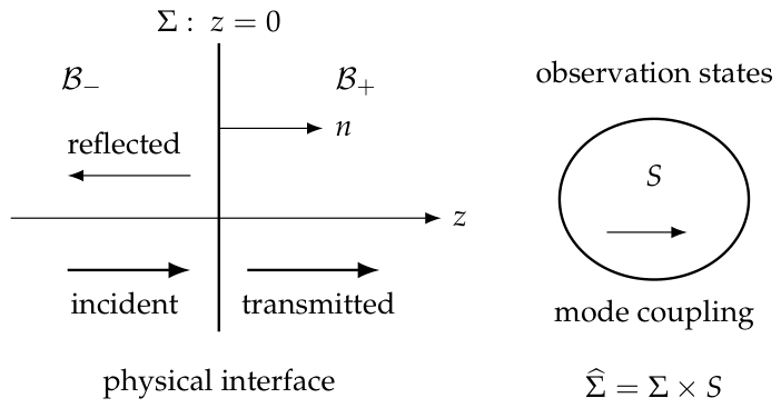
Figure 1.
The physical sheet and its observation-state domain. Jumps are taken across the physical normal coordinate z, while observation derivatives are tangent to . The two panels depict the physical and observation projections of the joint interface.
Figure 1.
The physical sheet and its observation-state domain. Jumps are taken across the physical normal coordinate z, while observation derivatives are tangent to . The two panels depict the physical and observation projections of the joint interface.
3. A Surface Action with a Continuous Potential Trace
3.1. Intrinsic Curvature and Constitutive Response
Assume that the tangential potential has a common trace on the sheet. Its curvature is
For a real local quadratic response, take
The same pair symmetries as in the bulk are assumed. With f dimensionally a curvature, p has the units of an excitation integrated over physical normal distance. For comparable bulk and surface tensor components, has one additional normal-length factor relative to . The geometry supplies the conversion between units of s and physical units; s need not have units of length.
Equation (17) specifies a local quadratic constitutive law. More generally, a nonlinear action depending on f gives and the same transition equation. Symmetric spatial kernels allow nonlocal response, while explicit dynamical sheet variables provide causal dispersive realizations.
The three intrinsic curvature sectors form
Accordingly, the response is a full block operator,
Here denote the physical, mixed, and observation two-form sectors, with independent antisymmetric components understood. Mixed curvature describes the field, whereas off-diagonal blocks describe constitutive coupling; neither requires the other to be nonzero. For , the observation two-form sector is absent, but the mixed sector remains.
3.2. Variational Transition Theorem
Theorem 1
(Continuous-trace dual-axis sheet conditions). Let the bulk fields be smooth on each side of and share the tangential trace a. Let the sheet response be defined by Eq. (17). Stationarity of the common bulk and surface action gives
The first condition holds for every physical and observation tangential free index. Its physical component is
Its observation component is
Proof.
The interface terms of the two bulk variations have opposite outward normals. Equation (10) therefore contributes
The sheet variation is
The sum vanishes for arbitrary , giving the first condition. The common trace implies , which gives the second condition. Splitting the tangential index gives Eqs. (22) and (23). □
The term describes intrinsic transport along the observation directions. Like the physical polarization current, it is a constitutive response evaluated on the joint bulk and sheet solution.
3.3. Conservation at the Sheet
Antisymmetry implies . Taking the divergence of Eq. (21), and using the normal bulk Maxwell equation, gives
This equation expresses surface-current conservation, including charge supplied by normal bulk flow, and follows independently from gauge invariance of the source terms. The induced current is intrinsically divergence-free.
For a compact observation space without boundary, or boundary conditions with zero observation flux,
Observation transport can therefore redistribute excitation and alter modal scattering while preserving the integrated charge. The integral identity (27) does not imply closure into a single physical mode.
3.4. The Thin-Layer Limit
The action derivation has an equivalent weak-limit interpretation. In the collar, the Maxwell equation for tangential B reads
Integrate over a layer . Suppose the one-sided normal excitations have finite limits and the tangential excess excitation and source have the limits
Under weak convergence for which tangential differentiation commutes with the limit, division by gives Eq. (21). Equivalently, the excitation distribution contains the tangential measure
Proposition 1
(Persistence of observation surface transport). Within the regular-sheet limit (29), an observation contribution to the physical excitation jump survives exactly through the distributional divergence . If the observation tangential excess excitation has a vanishing integrated limit and no other singular source is retained, this contribution vanishes.
Proof.
The observation part of the tangential integral in Eq. (28) converges to . If its integrated limit is zero, its distributional derivative is zero. If all relevant excess excitations are uniformly bounded in the layer, their integrals are and hence vanish. □
A finite may arise from a scaling of the tangential layer response or from a surface action retained after elimination of the layer fields. Mixed curvature in the surrounding bulk alone does not provide this scaling. Only the observation divergence of contributes to the excitation jump.
The limit excludes singular normal excitation: a surface measure in a normal component would generate a term upon differentiation. Such dipole layers lie outside Theorem 1. Continuity of the tangential potential also enforces continuity of its tangential curvature, restricting the magnetic-polarization response. The following construction allows this curvature to jump while keeping the action well defined.
4. Two Boundary Traces and the Complementary Transition Law
4.1. Gauge-Invariant Boundary Variables
Treat the bulk potentials and as smooth independent fields on their respective domains. Their tangential traces are and . Introduce a boundary phase and define
The gauge transformations
leave both and b invariant. The boundary phase compensates the difference between the local gauge choices; an optical readout phase would require a separate measurement model.
Consider the quadratic boundary action
Here , , and . We assume no bulk normal current in a neighborhood of the sheet. The corresponding excitations are
Both cross responses follow from the same term in the quadratic action, which fixes the relation between their coefficients.
4.2. The Paired Conditions
Theorem 2
(Two-trace dual-axis sheet conditions). Under the preceding assumptions, stationarity with respect to , , and φ gives
The complementary curvature condition is
If κ is invertible on the retained boundary subspace, the latter may be written
Proof.
Write . The sheet variation is
The bulk terms are . The coefficients of the independent traces are therefore
Their sum and difference give the first two equations of (36). Variation of gives . This is consistent with the normal bulk equation under the assumed absence of normal current. Finally, exterior differentiation of Eq. (31) gives because . Solving Eq. (35) for b gives Eq. (38). □
The first equation determines the excitation jump, while the second relates the average normal excitation to the potential-trace difference. With Eq. (37), the latter permits a tangential field-strength jump. For a harmonic transverse polarization, these laws correspond to electric and magnetic sheet currents. Observation indices occur in both; for example,
The bulk action in the two-trace theory is evaluated separately on smooth fields in the two domains, avoiding the ill-defined products of delta functions associated with a discontinuous distributional potential. The coefficients in Eq. (33) describe the effective layer response after its internal fields have been eliminated. Realizability and positive energy require constitutive conditions beyond pair symmetry.
Imposing before variation and using a common boundary trace recovers Theorem 1. A large positive quadratic penalty for b can yield the same limit in a stable realization. The continuous-trace response is thus a restricted member of the broader boundary description.
5. Recovery of Ordinary Maxwell Sheet Theory
5.1. A Preserved Electromagnetic Sector
Define the electromagnetic zero-mode sector by
Then . These conditions must be accompanied by preservation of the sector by the operators and boundary data. In particular, the bulk constitutive tensor must map physical two-forms to physical excitations. The sheet response must satisfy
on the physical sector, with . The coefficients are observation-independent on this sector. Initial data, incoming fields, and conditions on S are assumed to preserve it.
A constant observation section removes the differentials from the pullback but leaves observation derivatives in the joint Maxwell equations. Sector preservation is therefore a stronger requirement. Even at zero observation wave number, an s-independent can have nonzero .
Theorem 3
(Consistent ordinary-sheet recovery). Suppose the bulk and sheet operators preserve the sector (42)–(43), and the physical scattering problem is uniquely determined by compatible data. The restricted field equations are the ordinary four-dimensional Maxwell equations, and the restricted sheet equations are
for the continuous-trace class. In the two-trace class they are supplemented by
The omitted observation-index equations are satisfied identically. For compact S with finite volume, reduction of the common action and variation of the reduced action give the same physical equations.
Proof.
The curvature and excitation have only physical components in the preserved sector. The observation divergence in Eq. (12) vanishes, while the observation free-index equation has both sides zero. Equations (21) and (36) reduce to (44) and (45); all terms with an observation index vanish by hypothesis. The physical curvature identities are the ordinary Bianchi identities.
If the coefficients and retained fields are independent of s, integration over S multiplies the physical bulk and sheet action by the common volume . This overall factor cancels in the Euler equations. Equivalently, it may be absorbed into the four-dimensional electromagnetic normalization and the integrated sheet coefficients. Thus reduction commutes with variation. Uniqueness ensures that compatible physical data select this restricted solution. □
A constitutive block that maps physical curvature into or may source an observation-index equation even under zero-mode incidence. Closure of the physical sector must therefore be established from the full boundary equations.
5.2. Relation to Electric and Magnetic Polarization GSTCs
In the ordinary sector, the excitation and tangential-curvature jumps can be expressed in the standard electric and magnetic field variables. For an identical isotropic medium on both sides, a sheet with polarization moments and obeys [1,2]
Here no additional free sheet sources are included. The harmonic convention used later is , so becomes .
Equations (44) and (45) give the intrinsic variational form of these excitation and curvature jumps. Each boundary action selects a constitutive subclass. The continuous-trace action imposes , whereas the two-trace action supplies complementary magnetic response through b. Appropriate derivative-dependent boundary operators can encode normal dipole-gradient terms. The recovery theorem applies to the specified response operator without assuming a microscopic realization of arbitrary susceptibilities.
For a uniform transverse polarization with , the correspondence is especially direct. If and , then
With , the magnetic sheet admittance is . A kinetic electric sheet coefficient ℓ gives the electric admittance . Both are ordinary sheet responses when observation coupling is absent. The dual-axis extension adds independent observation equations and observation-index response components while retaining this physical limit.
6. Surface Response of a Minimally Coupled Projector
The transition conditions relate the normal excitation jump to the surface response. To determine that response, we derive the sheet current from a minimally coupled projector field. The resulting constitutive law also clarifies which couplings require additional material dynamics.
6.1. Thin-Layer Action and Induced Current
Let act on a finite-dimensional response space, and let be the electromagnetic generator in that space. The electromagnetic connection remains an independent field. Define
where the first pairing is for Hermitian matrices and the second for anti-Hermitian matrices. Consider the parent term
This term specifies material dynamics beyond the PODA state geometry. Its representation and coefficient are constitutive inputs.
In a product collar, assume that the tangential fields converge strongly enough for the weighted quadratic action to pass to their common trace, while the weighted normal-gradient action tends to zero. If
the retained action is
Here is the induced Lorentzian pairing, with positive coefficients in every nontemporal direction. A bounded parent coefficient with bounded gradients gives . A finite sheet contribution therefore requires a nonzero integrated material weight, as in Section 3.4. The limit (53) applies when the normal-gradient contribution vanishes; any surviving normal projector texture must be retained separately.
Using and cyclicity of the trace gives
Projector variations have the constrained form and give
It implies when no normal projector current crosses the sheet. For this action alone, the Maxwell interface equation becomes
Curvature-dependent material terms add to the left-hand side. The current is found by solving the coupled equations for P and a.
Proposition 2
(A neutral representation). If throughout the admissible projector configuration family, the minimal term (51) produces no electromagnetic current. At a homogeneous commuting background with vanishing connection, it produces no linear electromagnetic response.
Proof.
The electromagnetic variation contains the factor , so it vanishes identically on a commuting family. At a homogeneous background , the quadratic kinetic term depends on the connection perturbation only through , which vanishes when . □
The proposition concerns the minimal projector coupling. Nonlinear excursions into charged directions and polarizability from other gauge-invariant material terms remain possible.
6.2. Causal Response About a Charged Background
Take constant , a homogeneous , and zero background connection. Let
The Hermitian matrix R is tangent to the projector manifold. Write the tangent perturbation as , with . Because R is constant, the orthogonal fluctuations decouple from a at quadratic order, leaving
It is invariant under , . Its equations give
On a flat stationary sheet, choose zero initial response data and fields vanishing sufficiently far in the past. Retarded evolution then yields
The inverse is defined by the hyperbolic initial-value problem, so no algebraic inversion of static or gauge zero modes is required. The action is varied with retained, and the retarded condition is imposed on the resulting equations. Gauge transformations must preserve the preparation or transform the initial response data together with the potential.
For constant coefficients the derivatives commute with this retarded solution, and . Therefore the same response can be expressed as
This constitutive operator is nonlocal in time and in the tangential state variables. For a varying , the response follows from the weighted equation , which replaces the constant-coefficient construction (61).
The energy is explicit before the response variable is eliminated. In coordinates with , positive, set and . Then
Here and below i runs over physical and observation nontemporal tangent directions. The response equation gives , whereas . After removing edge flux,
The bulk contributes the opposite exchange term, so the combined energy is conserved. The causal constitutive law describes this lossless exchange with the retained response field.
6.3. Transverse Response and Local Mode Closure
In flat coordinates with and no off-diagonal y components, take independent of y and all other components zero. Then . With zero initial projector perturbation, and
The homogeneous charged projector produces a stiffness response diagonal in the observation eigenbasis, with modal amplitudes
An incident zero mode remains in that mode. The off-diagonal kinetic coupling in Section 7 therefore requires a different material response.
A nonuniform material density mixes modes through the local stiffness operator . Its relation to exact two-mode closure is constrained by the following proposition, which also applies to a local kinetic multiplier.
Proposition 3
(Local response and exact two-mode closure). On the circle, let and let be multiplication by a scalar local coefficient . If , then m is constant. Hence this local multiplier cannot produce nonzero off-diagonal coupling in an exactly invariant E.
Proof.
Since , invariance first gives . Writing and ,
The last component lies outside E, so . □
Exact finite-rank coupling can be obtained from a nonlocal kernel or additional dynamical response fields. Their coefficients must be determined by the corresponding material action. The minimal projector term yields the causal operator derived above, while more general metasurface responses require further constitutive data.
7. An Exactly Closed Observation-Mode Sheet
7.1. A Transverse Realization of the Parent Action
The following transverse realization permits an exact modal calculation. Let S be a circle with dimensionless coordinate and normalized measure . For constant orthogonal bulk coefficients, take the potential
In this transverse gauge, the nonzero curvature components are
With constant coefficients and fields independent of y, the remaining Maxwell free-index equations vanish. The transverse equation therefore defines a consistent solution sector of the full first-order Maxwell system.
After division by a fixed positive normalization, the action per unit physical transverse area is
Its equation is
The positive coefficient h sets the conversion between observation-coordinate derivatives and temporal and spatial units.
The two retained observation profiles are
They have observation eigenfrequencies
The nonzero profile is the even combination of the observation Fourier labels . These labels describe variation along the observation axis and carry no physical transverse wave number.
7.2. A Finite-Rank, Gauge-Invariant Sheet Response
Define the sheet modal traces
Consider the continuous-trace action
where
The response is nonlocal on S and local in physical time. Its constitutive coefficients are fixed before the frequency response is calculated.
A gauge-invariant extension to the full sheet curvature is obtained by replacing with and in the stiffness term with , where . Integration by parts on the circle gives . Equation (74) is therefore the transverse restriction of an action built from gauge-invariant curvature components.
Its electric kernel is
Both this kernel and the stiffness response annihilate every profile orthogonal to . Since the bulk observation operator also preserves their span, the two profiles form an exact invariant subspace. Higher cosine modes and all sine modes are decoupled spectators.
The sheet excitations in this sector are
Equation (21) gives
The last term is the retained observation-direction surface divergence and vanishes on the constant observation profile.
The off-diagonal kinetic coefficient is a material parameter that couples the two profiles. Its value and physical realization must be supplied in addition to the PODA field structure. Observable conversion is conditional on that realization of the observation-state response.
7.3. Positive Energy and Stationarity
Proposition 4
(Energy conservation of the mode-coupling sheet). For finite-energy solutions with no incoming flux at infinity,
The source-free model has no nontrivial finite-energy exponentially growing solution.
Proof.
Multiplying Eq. (70) by gives the local balance with normal flux and observation flux . The circle integral removes the observation-boundary term. Adding the two half-space integrals leaves at the sheet. By continuity of and Eq. (78),
A nontrivial exponentially growing field has a growing positive bulk kinetic energy, contradicting conservation. □
The sheet stores energy without loss. Its stationary coefficients make scattering diagonal in temporal frequency: observation-mode conversion changes the normal wave number at fixed , while the temporal frequency remains unchanged and no external modulation supplies power.
The conserved flux is the Noether flux of the joint electromagnetic action. Interpreting its normalization as laboratory power requires independently calibrated preparation and readout of the observation modes.
8. Local Sheet Response from a Stable Projector Equilibrium
The parent projector action (53) also determines a local mode-coupling law once the material representation and boundary data are specified. We construct a two-component realization, derive its equilibrium response, and retain the full set of electromagnetic observation modes coupled by that response.
8.1. Rank-one Representation and Field Equations
Let be the Pauli matrices and choose
This rank-one representation defines the material response variable. We use the same positive action normalization as in the transverse Maxwell sector. In polar coordinates,
The identities and turn the retained action into
Independent variation gives
The current and projector dynamics follow from the same action. The electromagnetic response of a nonuniform equilibrium is therefore obtained by expanding about the corresponding projector solution.
8.2. Instability of the Periodic Meridian
On an observation circle , the meridian , , with solves the static projector equation. Its electromagnetic current vanishes because is orthogonal to . However, consider the periodic unit-vector variation
At fixed zero connection, . Zero initial velocities and electric fields satisfy the charge constraint, so this perturbation is an admissible energy-lowering direction. The periodic background is thus energetically unstable. The fixed-connection transverse Jacobi operator has a negative constant mode, although the growth spectrum of the coupled system also includes electromagnetic perturbations.
Fixed observation-state endpoints provide a stable equilibrium of the same kinetic action, without an additional stabilizing potential.
8.3. Interval Equilibrium and Energy Minimum
Take with normalized measure , and fix the projector endpoints
These endpoint values specify the preparation on the observation-state interval. Let be constant, with unit physical y pairing and no off-diagonal y entries. The background
solves the projector equation and has in every direction. Hence it also solves the background Maxwell equations.
Theorem 4
(Energetic stability of the interval background). With the endpoint data (89), constant positive projector weight, and electromagnetic boundary data that supply no work, Eq. (90) attains the global static minimum of the coupled Maxwell–projector energy per unit physical transverse area. In the normalized observation measure,
The full energy is nonnegative relative to this minimum. Gauge-equivalent configurations need not be distinguished by the bound.
Proof.
The gauge-invariant angle is the spherical distance from . Since the generator rotates only the azimuth, almost everywhere. The Lipschitz property of the distance function extends this inequality to the north endpoint, where the polar chart is singular. Cauchy–Schwarz gives
All other projector kinetic and spatial energies, and the Maxwell energy, are nonnegative. The background has zero field strength, constant polar derivative, and zero covariant azimuthal derivative, so it attains the lower bound. □
Stability is relative to the fixed endpoint preparation. At fixed connection, the transverse Dirichlet Jacobi eigenvalues are , , with lowest value . The joint energy bound establishes stability while allowing the electromagnetic field to vary.
The electromagnetic endpoint data are specified separately. We impose on the transverse field to remove Maxwell flux through the observation edges, together with at the endpoints. With the projector endpoints fixed, these conditions give and zero projector edge energy flux. Gauge transformations must preserve the endpoint projectors, boundary conditions, and prepared initial data; at both ends is sufficient.
8.4. The Nonlinear Interface and Its Linear Response
For the transverse field , independent of y, with all other tangential components zero, solves the phase equation exactly. The common action gives
Off the sheet, u obeys Eq. (70), now on the interval. The corresponding retained energy is
The energy derivative is , which the bulk balance cancels. Equations (93)–(94) thus describe the coupled evolution of the electromagnetic field and projector.
For initially unperturbed projector data and a weak transverse field, on fixed time intervals. Consequently
The equilibrium and generator fix the response profile, while the integrated material weight sets its scale. The stationary scattering calculation below describes the linear response of the coupled system.
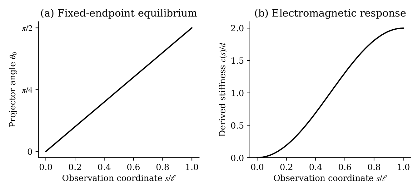
Figure 2.
Projector equilibrium and induced sheet response. Fixed north-pole and equatorial endpoints determine the quarter-meridian angle . The minimal coupling gives , with material scale d defined in Eq. (96).
Figure 2.
Projector equilibrium and induced sheet response. Fixed north-pole and equatorial endpoints determine the quarter-meridian angle . The minimal coupling gives , with material scale d defined in Eq. (96).
8.5. Local Coupling in the Observation Basis
The electromagnetic Neumann basis is
Let . Product-to-sum identities give the full matrix
with every other entry zero. The parent equilibrium fixes the ratio of each neighboring coupling to the diagonal. The coupling acts through stiffness; the off-diagonal kinetic coefficient is absent from this minimal transverse response.
The local multiplier is nonnegative, so every finite compression is positive. In fact its eigenvalues are
The first off-diagonal entry couples modes 0 and 1, and successive entries extend the coupling through the entire chain. No nontrivial finite initial segment is invariant, so a finite-mode calculation requires controlled elimination of the remaining profiles.
8.6. Scattering and Power in the Full Mode Chain
For left incidence in mode 0, set
We take the outgoing square root in every open and closed mode and define threshold amplitudes by the outgoing limit. Although the matrix is infinite, only finitely many modes carry normal power at a given frequency. At a nonsingular finite cutoff, tridiagonal elimination gives
The finite fraction ends with . The closed tail selects its unique infinite outgoing limit.
Uniqueness follows from the matching form. Away from thresholds,
The diagonal term grows with n, while the multiplier C is bounded, giving a well-defined limit of the finite matching solutions. At a threshold, the imaginary part of the homogeneous matching equation gives for . The nonzero neighboring entries then imply successively. Eliminating a sufficiently high, coercive closed tail reduces existence to the resulting finite nonsingular system. This argument includes exact thresholds.
With zero-mode incident power , define
The closed channels contribute zero power. Multiplying the matching equation by and taking its imaginary part proves
The bound follows from for the symmetric continuous-trace class; it need not hold for the complete two-trace family. Eliminating closed modes leaves a real symmetric effective stiffness on the open modes, whose flux-normalized scattering matrix is unitary and reciprocal.
8.7. An Error Bound for the Omitted Modes
Every conservative finite cutoff satisfies power balance, so truncation accuracy requires a separate estimate. The local chain admits an explicit error bound. Use and , and divide the matching equation by . Write d for in the next proposition only, so and .
Proposition 5
(Tail estimate at spectral thresholds). Retain modes , with and . Define
If , let
Extending by zero gives
The estimate remains valid when any retained mode is exactly at threshold.
Proof.
The omitted tail is entirely closed. Let and let denote its first basis vector. The tridiagonal form gives
For the first inequality, the tail stiffness is b times the sum of the first-component square and the squared successive differences. The remaining two inequalities follow by positive-operator comparison and .
Eliminating the tail adds to , with . The rank-one inverse identity gives
Since , this bounds the head error and its zero-mode component. The tail equals , whose norm is bounded by Eq. (109). Head and tail occupy orthogonal sequence components, giving the stated full bound. □
The estimate applies to exact Galerkin solutions. Once arithmetic precision dominates the tail error, numerical solve residuals must be assessed separately. The denominator measures the conditioning of the correction to the retained modes; increasing N resolves an inconclusive bound.
8.8. Scattering Results and Modal Convergence
Figure 3 shows scattering for using the equilibrium-derived matrix. These values illustrate the dependence on the integrated material weight, which remains a constitutive input. The observation thresholds occur at . Each newly open mode carries a share of the converted power, while evanescent modes modify the response below threshold.

Table 1.
Modal convergence at . Maxima are taken over , including two exact thresholds. The bound (108) is analytic; the solution serves as an independent numerical comparison. The zero-mode difference for is below the double-precision comparison scale.
Table 1.
Modal convergence at . Maxima are taken over , including two exact thresholds. The bound (108) is analytic; the solution serves as an independent numerical comparison. The zero-mode difference for is below the double-precision comparison scale.
| N | Analytic bound | ||
| 4 | |||
| 6 | |||
| 8 |
The full modal amplitude error decreases from at to at on this test set, within the analytic bounds. The maximum power-balance residual across the displayed grid is below . Open-port unitarity has the same residual scale at ten additional frequencies per material value, including four exact thresholds. Matrix inversion and continued-fraction evaluation give amplitudes agreeing at that scale. Experimental comparison requires an independently identified observation-state preparation and readout.
9. Finite-Thickness and Causal Material Realizations
9.1. A Positive-Energy Finite-Layer Realization
The kernel (76) admits a finite-thickness realization with a controlled sheet limit. Retain , , so that the stiffness has the stated mixed-curvature extension. Let denote the two modal amplitudes throughout the layer, set , and take for and zero outside. The action is
Applying the curvature-based extension of Section 7 at each z gives a gauge-invariant layer action. The conserved energy is obtained by changing the signs of its gradient and stiffness terms and is nonnegative for . The bulk operator and layer response preserve the two profiles at every thickness, so modal closure holds before the sheet limit is taken. The construction realizes a kernel whose constitutive coefficients remain material inputs.
For harmonic fields define and . Variation of Eq. (111) gives
The exact transfer of the state between the left and right layer faces is
Theorem 5
(Controlled continuous-trace limit). For fixed finite matrices and bounded frequency intervals,
Consequently the finite layer converges to and . Its scattering amplitudes converge at this rate on sets where the limiting matching matrix remains uniformly invertible.
Proof.
Write the exponent in Eq. (113) as , with
Since , . Continuous differentiability of the matrix exponential, with a uniformly bounded derivative on bounded matrix sets, gives the transfer estimate. Its upper and lower block equations yield the interface laws. Uniform invertibility of the matching system then carries the same estimate to the scattering amplitudes. □
The amplitude estimate includes a finite threshold limit when the matching matrix is nonsingular. Flux normalization for requires a separate limiting treatment. Uniformity is restricted to the stated nonsingular bounded-frequency sets and excludes resonances or frequency ranges increasing with .
9.2. The First Correction at the Layer Center
To identify an effective sheet at the layer center, remove the exterior propagation by defining . Differentiation at gives
The expansion holds without assuming that and V commute, since the derivative is . Centering both exterior reference planes cancels the free propagation terms:
The corrected jump therefore yields second-order scattering accuracy under the same nonsingularity condition. For , the correction contains terms. Its validity is that of a finite-band asymptotic approximation to the positive-energy slab, rather than a global higher-derivative material action.
The retained contrast modifies the thinness criterion. Internal response is controlled by the characteristic dimensionless measures and , in addition to exterior propagation. Even when is small, a large material response or poor conditioning of the matching problem can limit the sheet approximation.
9.3. Auxiliary Response Variables and Retarded Elimination
A causal dispersive response can recover the time-local kinetic kernel at low frequency. Retain a real response vector with action
where , , and is the stiffness of the two-mode model. The coupling uses the gauge-invariant electric curvature profiles representing , while the stiffness uses the mixed-curvature profile defined above. These auxiliary variables specify a material completion distinct from the minimal projector term. Retaining response oscillators before elimination provides an action-based description of dispersion [6]; their coupling here also acts on observation profiles.
Independent variations give
The velocity-linear interaction cancels from the conserved energy:
Equations (119)–(120) give , canceled by the bulk energy balance.
For zero initial response, let be the retarded inverse of . Its time-domain kernel is
Eliminating after variation gives
Away from unresolved material poles, the scattering formulas below apply with V replaced by . The causal prescription is imposed on the solution after independent variation of the retained fields. It therefore defines a response operator while the stored-energy argument remains a property of the retained equations; a retarded kernel is not inserted into a real single-field action.
At low frequency,
Every positive semidefinite matrix L admits this factorization, for example , , , . A chosen kernel thus admits a passive dynamical realization once the oscillator parameters are specified. In this example , and replacing the lossless dispersive response by L gives the matrix error relative to the static kernel for .
9.4. Absorption and Outgoing Observation Modes
A passive reservoir can be represented at the reduced level by adding to the left of Eq. (120), where . This additional reservoir specification introduces damping into the otherwise conservative dynamics of Eq. (118). The retained bulk and response energy satisfies
Writing , the algebraic identity
gives for positive real frequency. The electric admittance has Hermitian real part . Material absorption can therefore be separated from power carried by outgoing observation modes.
For unit zero-mode incidence, the absorption fraction is
The balance resolves the zero-mode power deficit into conversion and absorption. Conversion counts power in additional open outgoing modes, while absorption counts power delivered to the reservoir. A restricted measurement may combine these distinct contributions into apparent loss.
Figure 4 compares the layer approximation with the exact slab and illustrates a causal realization of the same dimensionless static kernel. The oscillator parameters are independently specified material inputs for this forward calculation.
10. Scattering from the Two-Mode Sheet
10.1. Outgoing Solutions
For the two-profile response, write and . The normal wave numbers are
Below threshold , with . Incoming amplitudes are allowed only in open channels. Put and write
The outgoing factors decay away from the sheet in a closed channel. Continuity and the jump condition give
Thus
where and . These matrices give the exact amplitudes for the specified response.
For zero-mode incidence , define
The amplitudes are
Here . Setting gives
This recovers the ordinary electric-sheet amplitudes. The observation stiffness enters the scattering response only when the additional mode is populated.
10.2. Flux and Reciprocity
The period-averaged normal power of an open-channel traveling amplitude is
Integration over S removes cross terms by observation-profile orthogonality. Evanescent amplitudes have zero average normal power at infinity.
Theorem 6
(Lossless modal scattering). For real away from thresholds,
where is the positive wave number on open channels and zero on closed channels. When both channels are open, the flux-normalized two-sided scattering matrix is unitary. For real symmetric and identical half-spaces, it is also symmetric.
Proof.
The normal flux difference at the sheet is proportional to , which vanishes for . The closed-channel fields decay at infinity, giving Eq. (137). For open channels put and . Then
The real symmetric Q has an orthogonal eigenbasis. In that basis each eigenchannel is a scalar reactive sheet. Therefore
□
For zero-mode incidence define
The factor two accounts for observation-mode power on both physical sides. Below threshold, . Equation (137) becomes
Corollary 1
(One-sided conversion bound). For this lossless continuous-trace sheet in identical half-spaces,
Proof.
Since ,
Substitute into Eq. (141). □
The bound depends on the continuous trace, identical half-spaces, one-sided incidence, and the specified channels. The two-trace action changes the continuity relation; asymmetric media, coherent two-sided incidence, or additional physical channels likewise require their own bounds.
10.3. The Observation Threshold
Below threshold the additional mode has
A nonzero then describes an evanescent response that stores energy and carries zero outgoing power. Above threshold,
Its physical normal group velocity is smaller than that of the zero mode. If has a finite nonzero threshold limit, the conversion has the generic onset
A threshold pole or a coupling zero changes this scaling and requires separate treatment.
With one observation coordinate, the example has no local curvature. Its additional field structure consists of the mixed component and the observation spectrum. Stationary conversion changes the normal wave number at fixed .
10.4. An Illustrative Response
Use the frequency scale , normal-length scale , and a fixed action normalization to set . The dimensionless sheet coefficients are
Choose
The kinetic eigenvalues are and . The coefficients are illustrative material inputs selected independently of measurements or curve fitting.
Figure 5 and Table 2 follow from Eq. (134). At , the observation amplitude is substantial but carries no outgoing power. At , the open observation channel carries approximately of the incident modal power. On the displayed grid the conversion maximum is about near , consistent with Corollary 1.
The accompanying program evaluates 1202 frequencies and compares the explicit amplitudes with the matrix solution. A fixed-seed ensemble of 200 additional positive-energy reciprocal sheets provides a further numerical comparison of the flux normalization. For the displayed example, the maximum power-balance residual is below in double precision. These calculations establish numerical agreement with the analytic model; experimental testing requires the calibration described below.
11. Eliminating the Observation Channel
The second row of the scattering equation gives . For , the first row consequently reduces to
This Schur complement eliminates the observation block. At a pole of the reduced representation, the amplitudes are obtained from the full matrix formula (132) or its limit.
Define
The sign follows from and : the electric sheet current is .
Proposition 6
(Exact equivalence on zero-mode ports). At regular frequencies, a conventional sheet with admittance has exactly the same zero-mode reflection and transmission. Below threshold this admittance is reactive. Above threshold its conductance is nonnegative and represents power transferred into the eliminated outgoing mode.
Proof.
Equation (150) is the ordinary admittance-sheet formula. Below threshold, is real; hence is real. Above threshold,
The apparent dissipated fraction of the zero-mode ports is
□
The full system remains lossless, while its restricted ports exhibit apparent loss as the omitted open channel carries energy away. When a physical transverse wave number is retained, also produces spatial dispersion in the effective response. An ordinary nonlocal boundary operator can represent this projected response.
The equivalence sets the scope of a port measurement. The joint model specifies an observation spectrum, a conversion amplitude, and mixed curvature, yet elimination of the additional variable allows an ordinary boundary model to reproduce . A dispersive reflection curve or apparent loss alone therefore cannot identify an independent observation axis.
A readout of and the response to independently prepared observation modes require preparation and readout maps in addition to the effective admittance. These maps supply further observables for comparing specified models whose ordinary port responses coincide.
For a general linear boundary problem, partition the unknowns into retained and eliminated variables:
Where the outgoing inverse exists, the retained equation is
The reduced operator can have memory and spatial dispersion. The two projections retain their distinct roles in the full theory, although those roles generally cannot be reconstructed from the restricted port operator.
12. Observation Sections and Mode-Resolved Measurements
12.1. The Field on a Section
An observation field defines . Its pulled-back curvature is
Exterior differentiation commutes with pullback, so . The full mixed and observation-index equations are still needed to determine the joint solution.
Hold that solution fixed and vary a constant section to . Equations (5) and (155) give
Equation (156) gives the exact first-order response to a section variation. If the control also perturbs the joint field, its field variation contributes separately.
For a constant section in the transverse model,
Figure 6 shows three sections of the same transmitted joint solution. Their amplitudes differ through the readout combination, while relabeling the section leaves the joint electromagnetic power distribution unchanged.
12.2. A Mode-Resolved Test
A physical implementation requires accessible observation states, a calibrated readout, and a preparation that preserves the specified physical input. Independent determination of the observation operator and sheet coefficients gives S, h, L, and D experimental meaning, allowing their scattering predictions to be tested against separate data.
Three calibrated sections of the two-profile model give
The last relation provides a redundant consistency test. Failure indicates an incompatible readout or additional profile contributions, while agreement does not exclude every higher observation mode. The same equations apply to harmonic electric amplitudes with the common factor .
With this calibration, the model predicts the wave number (129), threshold (72), amplitudes (134), and flux relation (141). The reconstructed mode decays away from the sheet below threshold; above threshold, its propagating phase and calibrated power account for the zero-mode deficit. Reversing an independently established reverses while leaving zero-mode powers unchanged. Testing these joint-mode predictions requires independently specified coefficients rather than an admittance refitted at each frequency.
For the equilibrium-derived interval sheet, the local coupling excites the full basis (97). Recovering its modal amplitudes requires a calibrated field resolved over observation states and projection onto those profiles. The three-sample relation above applies to the separate two-profile model; reconstruction of the full local chain requires the corresponding full-basis projection.
A comparison with conventional sheet scattering requires the same measured incident field, material geometry, bias, temperature, propagation path, instrument phase, and readout protocol. Since changes in these controls also affect ordinary scattering, the null prediction must come from a specified conventional model under matching conditions. Conventional electromagnetic systems can also exhibit phase shifts and spectral thresholds.
Agreement would support the specified coupled surface model. Establishing the operational independence of S requires additional evidence for the two state roles alongside mode-resolved scattering, including comparison with conventional realizations that contain internal modes.
12.3. Observation Loops and Phase Coupling
For , can be nonzero. If a coherent readout degree of freedom is specified to parallel-transport with derivative , its closed-loop comparison contains
For a contractible loop, Stokes’ theorem identifies the exponent with observation-curvature flux. Relating this Wilson factor to a measured optical phase requires a specified readout coupling and transport law in addition to the Maxwell sheet action. The one-dimensional scattering example provides no numerical prediction for this loop phase.
13. Consequences for Surface Theory
The interface laws place physical polarization currents and observation-direction transport within the same variational balance. Two independent boundary traces extend this description to curvature jumps while preserving separate gauge choices on either side. When the bulk and boundary operators preserve the physical electromagnetic sector, both constructions reduce consistently to ordinary Maxwell sheet theory.
The constitutive response can couple physical, mixed, and observation curvature sectors, subject to energy, gauge, and realizability conditions. Bianchi identities constrain the admissible fields but do not select a susceptibility. Consequently, inverse design requires a solution of the coupled bulk and boundary problem, with these identities enforced throughout.
The finite-rank example shows how a static sheet couples a constant observation profile to a nonconstant one. The additional mode has its own propagation threshold and normal wave number, and its excitation produces mixed curvature . Frequency is preserved. The full sheet is lossless, although a measurement restricted to the zero-mode ports records a power deficit once the additional channel opens.
The parent projector action yields a causal current and positive surface energy. Its charged sector depends on the chosen representation, and a homogeneous background gives diagonal transverse response. Fixed endpoint preparation on an observation interval instead selects a stable equilibrium with nonuniform local stiffness. The resulting coupling ratios, and for , follow from that equilibrium. The overall material scale remains an independent parameter.
Nonconstant local multiplication cannot close exactly on the two-mode subspace of the circle, as Proposition 3 shows. The interval model therefore requires the full modal chain, with truncation controlled by Proposition 5. The nonlinear equations also delimit the weak-field calculation: on fixed time intervals, projector displacement begins at second order in field amplitude and changes the current at third order.
The finite-layer and auxiliary-variable constructions complement this local response model. For a specified finite-rank kernel, they establish the sheet limit, quantify the leading thickness correction, and distinguish stored energy from reservoir loss. A device realization would additionally require material parameters, physical endpoint preparation, and calibrated maps between observation modes and measured records.
Channel elimination explains why ordinary reflection and transmission alone cannot provide those maps. An effective admittance reproduces the restricted port response while concealing the unresolved modal amplitudes. Independently prepared and resolved observation modes are therefore needed to test a specified joint-state realization.
14. Conclusions
The common dual-axis Maxwell and sheet action gives
The observation contribution is the divergence of the finite integrated observation response retained in the thin-layer limit. An action with two gauge-compensated potential traces also permits tangential curvature jumps. Ordinary Maxwell interface theory is recovered when the physical electromagnetic sector is preserved by the constitutive operators and the initial and boundary data.
The minimally coupled projector action provides a surface response derived from explicit field dynamics. A stable interval equilibrium fixes the shape of its local stiffness and the relative neighboring-mode couplings, leaving one material scale. The nonlinear equations retain projector backreaction, while an analytic tail estimate controls weak-field scattering at and between channel thresholds. For a separate finite-rank kernel, the finite-layer construction quantifies thickness corrections and the auxiliary variables give a causal realization with explicit energy storage and absorption.
Analytic reflection, transmission, and conversion amplitudes demonstrate the distinction between evanescent and propagating observation channels. Lossless scattering conserves flux; eliminating an open channel turns its outgoing power into apparent loss at the retained ports. The resulting ordinary admittance is exact on those ports, but it omits the preparation and readout information needed to resolve observation-state dynamics.
Data Availability Statement
The numerical results are theoretical calculations. The accompanying source package contains the code, fixed parameters, and tables required to reproduce them.
Appendix A. A Scalar Two-Trace Sheet
A single harmonic transverse polarization in identical media illustrates the complementary law without introducing an observation coordinate:
The first equation is the excitation jump; the second is the difference-of-traces response. With real and left incidence,
Writing and gives
Both ratios have unit modulus, so . As , and
Finite supplies the independent magnetic response and permits . The continuity-based conversion bound consequently does not extend to the entire paired sheet family.
Appendix B. Closure, Units, and the Exact Threshold
On the normalized circle, and . For arbitrary smooth periodic u,
The stiffness operator therefore has image spanned by . The electric kernel has image spanned by , and the bulk operator preserves both. This proves exact closure at all frequencies, including the closed-channel regime.
For dimensionless s and a normal coordinate measured in length,
These relations imply Eq. (147). The numerical example is dimensionless; a physical frequency and fabrication length require material calibration.
At , the observation channel has zero normal wave number and a singular incident-port flux normalization. The zero-mode input still has a finite scattering limit if . For Eq. (148),
This finite additional amplitude carries zero outgoing power. It explains the transmission minimum at channel opening. Flux-normalized numerical checks are performed away from the exact threshold.
Appendix C. Reproducibility
Three Python programs reproduce the numerical calculations and figures using NumPy, SciPy, and Matplotlib. The source files, fixed parameters, and numerical tables accompany the manuscript.
reproduce_scattering.py compares explicit, matrix, and Schur-complement amplitudes; checks channel power, profile orthogonality, and spectator projections; and tests reciprocity and unitarity on 200 fixed-seed positive-energy sheets.
reproduce_closure.py compares the exact slab with leading and corrected sheets, checks flux and symplectic preservation, and compares channel absorption with oscillator dissipation. The plotted convergence errors use five fixed frequencies.
reproduce_parent_chain.py checks the equilibrium current, commutator identity, modal matrix, and finite eigenvalues. It compares direct and continued-fraction scattering, verifies channel balance and selected open-port matrices, and evaluates the analytic tail bound. The numerical records distinguish solve residuals and arithmetic allowances from the analytic truncation estimate.
References
- E. F. Kuester, M. A. Mohamed, M. Piket-May, and C. L. Holloway, Averaged transition conditions for electromagnetic fields at a metafilm, IEEE Transactions on Antennas and Propagation 51, 2641–2651 (2003). [CrossRef]
- K. Achouri, M. A. Salem, and C. Caloz, General metasurface synthesis based on susceptibility tensors, IEEE Transactions on Antennas and Propagation 63, 2977–2991 (2015). [CrossRef]
- X. Meng, The Natural Dual-Axis Structure of Observation: Categorical Foundations and Consequences for Quantum Theory, preprint, version 3 (2026). [CrossRef]
- K. Achouri and O. J. F. Martin, Fundamental properties and classification of polarization converting bianisotropic metasurfaces, IEEE Transactions on Antennas and Propagation 69, 5653–5663 (2021). [CrossRef]
- F. W. Hehl, Y. Itin, and Y. N. Obukhov, Recent developments in premetric classical electrodynamics, in Proceedings of the 3rd Summer School in Modern Mathematical Physics, edited by B. Dragovich, Z. Rakić, and B. Sazdović (Institute of Physics, Belgrade, 2005), pp. 375–408; arXiv:physics/0610221 (2006).
- T. G. Philbin, Canonical quantization of macroscopic electromagnetism, New Journal of Physics 12, 123008 (2010). [CrossRef]
Figure 3.
Scattering of the equilibrium-derived local sheet. (a) Total two-sided conversion for three material weights. (b) Power in each outgoing mode at . Vertical dotted lines mark observation thresholds. The matrix (98) is retained through , including outgoing closed modes. The grid contains 1104 frequencies per material value and includes the exact first four thresholds.
Figure 3.
Scattering of the equilibrium-derived local sheet. (a) Total two-sided conversion for three material weights. (b) Power in each outgoing mode at . Vertical dotted lines mark observation thresholds. The matrix (98) is retained through , including outgoing closed modes. The grid contains 1104 frequencies per material value and includes the exact first four thresholds.
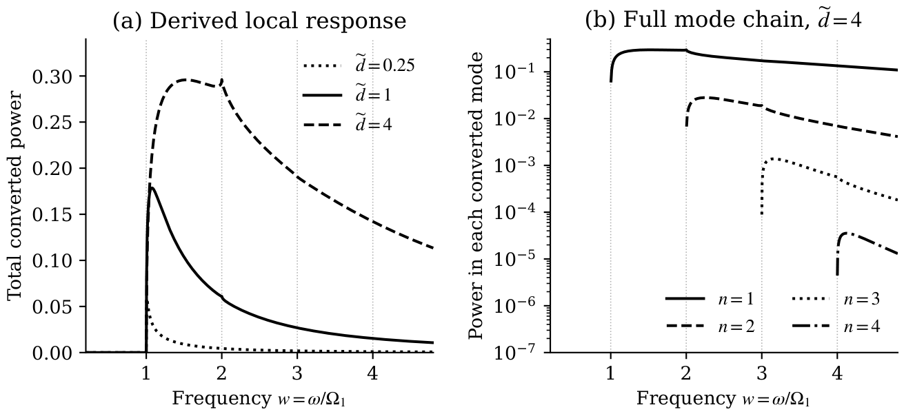
Figure 4.
Finite-layer and causal realizations of the specified response. (a) Maximum absolute error of the complex reflection and transmission amplitudes, over , relative to the exact rectangular slab. The estimated convergence orders are and for . All quantities are dimensionless as in Eq. (147). (b) Conversion for the instantaneous kernel and for auxiliary oscillators with , , , , . The damped case uses and displays absorption separately. The same as Eq. (148) are used in both panels. The finite-layer and damped channel balances have maximum residuals below on the stated grids.
Figure 4.
Finite-layer and causal realizations of the specified response. (a) Maximum absolute error of the complex reflection and transmission amplitudes, over , relative to the exact rectangular slab. The estimated convergence orders are and for . All quantities are dimensionless as in Eq. (147). (b) Conversion for the instantaneous kernel and for auxiliary oscillators with , , , , . The damped case uses and displays absorption separately. The same as Eq. (148) are used in both panels. The finite-layer and damped channel balances have maximum residuals below on the stated grids.
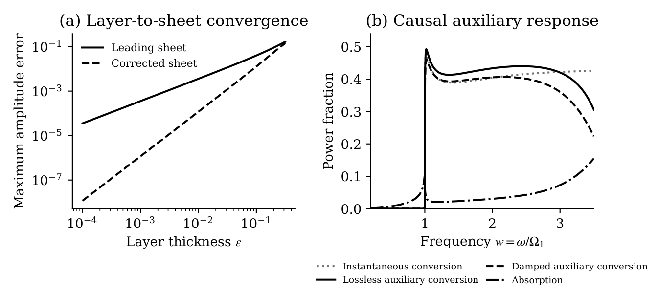
Figure 5.
Exact powers for Eq. (148). Solid, dashed, and dotted curves show , , and total two-sided conversion . The observation mode opens at . Below threshold its amplitude is evanescent and its outward power is zero. The powers sum to one.
Figure 5.
Exact powers for Eq. (148). Solid, dashed, and dotted curves show , , and total two-sided conversion . The observation mode opens at . Below threshold its amplitude is evanescent and its outward power is zero. The powers sum to one.
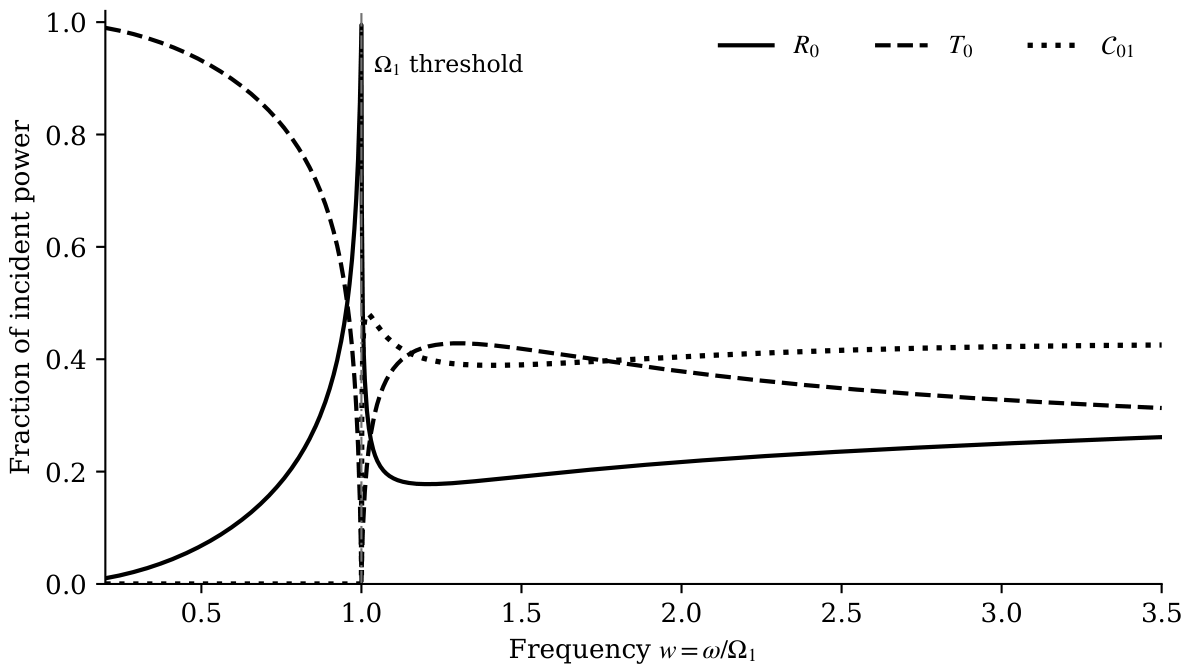
Figure 6.
Sections of the transmitted solution at . The upper panel shows the real field at for three constant observation states. The lower panel shows the transmitted modal magnitudes. Interference affects section amplitudes; those amplitudes are not the integrated modal powers of Figure 5.
Figure 6.
Sections of the transmitted solution at . The upper panel shows the real field at for three constant observation states. The lower panel shows the transmitted modal magnitudes. Interference affects section amplitudes; those amplitudes are not the integrated modal powers of Figure 5.
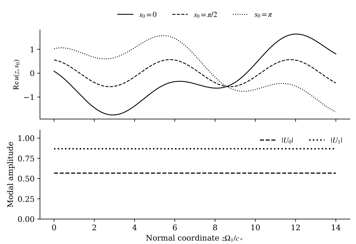
Table 2.
Calculated values. includes observation-mode power on both sides; is an amplitude. The unrounded power sum is one.
Table 2.
Calculated values. includes observation-mode power on both sides; is an amplitude. The unrounded power sum is one.
| w | ||||
| 0.60 | 0.103105 | 0.896895 | 0.000000 | 0.136983 |
| 0.95 | 0.477484 | 0.522516 | 0.000000 | 0.813210 |
| 1.05 | 0.218389 | 0.321940 | 0.459671 | 0.868205 |
| 1.50 | 0.191221 | 0.418735 | 0.390044 | 0.511517 |
| 2.50 | 0.235730 | 0.348298 | 0.415972 | 0.476373 |
Disclaimer/Publisher’s Note: The statements, opinions and data contained in all publications are solely those of the individual author(s) and contributor(s) and not of MDPI and/or the editor(s). MDPI and/or the editor(s) disclaim responsibility for any injury to people or property resulting from any ideas, methods, instructions or products referred to in the content. |
© 2026 by the authors. Licensee MDPI, Basel, Switzerland. This article is an open access article distributed under the terms and conditions of the Creative Commons Attribution (CC BY) license (http://creativecommons.org/licenses/by/4.0/).
Copyright: This open access article is published under a Creative Commons CC BY 4.0 license, which permit the free download, distribution, and reuse, provided that the author and preprint are cited in any reuse.