
Submitted:
30 September 2026
Posted:
01 October 2026
You are already at the latest version
Abstract
Flow in fractured porous reservoirs is coupled to rock deformation and heat transfer through pressure-dependent properties, temperature-dependent viscosity, and fluid exchange between the matrix and fractures. These interactions produce contrasting spatial and temporal scales that can complicate neural approximation of the governing equations. This study investigates a Fourier-feature physics-informed neural network (Fourier-PINN) for thermo-hydro-mechanical (THM) modelling of two-phase oil-water flow in a dual-continuum system. The formulation includes phase mass balances, quasi-static mechanical equilibrium, thermal constitutive relations, stress-sensitive permeability, and pressure-driven and imbibition-related exchange. An established Fourier feature map is combined with a weighted data-and-physics loss to approximate matrix pressure, fracture pressure, oil saturation in each continuum, and temperature. The assessment includes a comparison with a baseline PINN, residual diagnostics, field visualisation, and a parameter study. The reported comparisons show improved agreement with the reference data for matrix pressure, matrix oil saturation, and temperature, with R2 values of 0.923, 0.923, and 0.947, respectively. The reported extrapolation error decreases from 14.7% for the baseline PINN to 4.2% for the Fourier-PINN. Scenario comparisons suggest that fracture permeability and matrix-fracture exchange influence pressure communication and matrix oil mobilisation under the investigated conditions. The framework combines coupled physical relations, continuous neural approximation, and the interpretation of scenario results to provide a structured computational approach for analysing oil-water reservoir behaviour under the investigated conditions.
Keywords:
dual-continuum model
; thermo-hydro-mechanical coupling
; oil-water flow
; physics-informed neural network
; Fourier features
; matrix-fracture exchange
1. Introduction
1.1. Fractured Reservoirs and Coupled Transport Processes
Predicting oil–water flow in fractured reservoirs requires the representation of two interacting transport environments: a relatively low-permeability matrix that provides much of the storage, and a more conductive fracture system that redistributes pressure and fluid. The classical dual-continuum formulation of Warren and Root [1] and the anisotropic permeability description of Snow [2] established complementary foundations for modelling these systems. During production or injection, pore-pressure changes modify effective stress, while temperature changes influence fluid mobility and rock deformation. Poroelasticity [3] and the dependence of fracture conductance on aperture [4] therefore remain relevant to interpreting reservoir response. Figure 1 summarises the physical interactions considered in this study.
Recent work has expanded both the range of physical processes represented and the numerical resolution of thermo-hydro-mechanical (THM) modelling. Vaezi et al. [5] reviewed continuum and discontinuum approaches for fractured rock, emphasising that fracture representation, coupling strategy, parameter calibration, and scale must be selected together. Their synthesis shows why a model appropriate for distributed matrix–fracture exchange need not be appropriate for individual fracture propagation. Xu et al. [6] investigated multiphase THM behaviour in matrix-type shale oil systems, whereas Lee et al. [7] developed a phase-field formulation for propagating fractures under coupled thermal, hydraulic, and mechanical loading. These studies represent distinct modelling objectives: the former resolves coupled reservoir responses, while the latter explicitly addresses evolving fractures. The present work uses overlapping matrix and fracture continua and does not introduce a fracture-propagation model.
Two additional physical issues are important in low-permeability formations. Cheng et al. [8] combined stress sensitivity and boundary-layer effects in a pre-Darcy model, and their subsequent unified formulation [9] described the transition between nonlinear low-gradient flow and Darcy flow. These developments show that matrix mobility cannot always be represented adequately by a constant permeability alone. At the pore scale, Yang et al. [10] examined fluid–solid coupling using three-dimensional digital cores. Such resolved descriptions complement, but do not directly replace, continuum-scale constitutive laws. For two immiscible phases, matrix–fracture exchange also includes capillary-driven imbibition: the experiments and modelling of Hatiboglu and Babadagli [11] identify the importance of viscosity, wettability, rock type, and block geometry. Consequently, oil–water THM modelling must distinguish pressure-driven communication, phase redistribution, and stress- and temperature-dependent properties, even when the fracture geometry is represented in an averaged sense.
1.2. Recent Computational and Learning Approaches for Fractured Multiphase Flow
Conventional numerical simulation remains the reference framework for solving coupled conservation laws. Its computational demands arise from permeability contrasts, nonlinear phase mobilities, geometric complexity, and the repeated solutions required for parameter studies. Recent research has therefore pursued both improved physical discretisations and learned approximations that retain selected structures of numerical solvers. For example, Gimenez et al. [12] combined fine-scale representative-volume simulations with machine-learning-based upscaling in a pseudo-direct numerical simulation framework for highly fractured media. The fine-scale calculations provide effective transport properties for coarser reservoir models. This approach addresses the cost of resolving fractures through multiscale homogenisation, rather than by replacing all governing equations with a coordinate-based network.
A related line of research learns mappings between reservoir descriptions and flow responses. Wen et al. [13] developed U-FNO for multiphase-flow prediction, combining Fourier neural operators with a U-Net structure. Jiang [14] used graph neural networks to predict transient pressure and saturation in fractured systems represented by an embedded discrete fracture model, with graph connectivity accommodating unstructured spatial relationships. Chen et al. [15] embedded DeepONets in a physics-informed framework for production prediction in multiscale shale matrix–fracture systems. These studies show how operator learning and graph representations can incorporate information that is difficult to express with a simple coordinate input. They also clarify an important distinction: a Fourier neural operator learns a mapping between functions, whereas the Fourier features used here enrich the inputs to a neural approximation of a particular solution. The two methods share spectral ingredients but have different training tasks and generalisation requirements.
Physics-informed neural networks (PINNs) provide another route by incorporating differential-equation residuals and available observations into the learning objective [16,17]. Their appeal in subsurface applications lies in their ability to combine sparse information with governing relations in a single differentiable representation. However, the choice and numerical evaluation of physical residuals remain central. The recent review by Samarkanov et al. [18] documents the progression from Darcy-flow benchmarks to multiphase displacement, fractures, inverse problems, and coupled processes, while identifying validation and integration with reservoir simulators as continuing priorities. Thus, physics-informed learning is best assessed in relation to a specified physical model and computational task rather than treated as a universally faster replacement for conventional simulation.
1.3. Physics-Informed Simulation of Heterogeneous Flow and Coupled Fields
Several recent studies directly address the difficulty of learning two-phase flow in heterogeneous or fractured media. Yan et al. [19] developed an enriched PINN (E-PINN) with an embedded discrete fracture model, finite-volume residuals, hard initial and boundary constraints, and an implicit-pressure, explicit-saturation strategy. Their formulation uses discretised fluxes rather than automatic differentiation for spatial derivatives, enabling explicit treatment of matrix–fracture connections. Wang et al. [20] subsequently applied improved PINNs to a reinterpreted discrete fracture model for single-phase flow and contaminant transport; finite-element-based residual evaluation addresses difficulties associated with fracture-localised coefficients. These approaches demonstrate that fracture treatment and conservation structure can be as important as the network architecture itself.
Training strategies for reservoir models have also become more specialised. Lin et al. [21] introduced layer-specific constraint learning for enriched PINNs, using differentiated parameter updates to improve two-phase-flow predictions across time steps. Zhu et al. [22] proposed an adaptive-wavelet network for oil–water reservoir simulation, combining a pressure loss formulated using finite volumes with an explicit saturation update. In a complementary direction, Zhang et al. [23] investigated multiphase displacement with dual shocks and interphase solubility. Their work highlights the importance of the transport formulation when moving fronts or multiple discontinuities are present. Together, these studies show that accurate pressure and saturation prediction depends on the interaction of representation, time advancement, physical constraints, and the character of the displacement front.
Coupled thermal and mechanical problems add further requirements. Amini et al. [24] formulated PINN solutions of THM processes using dimensionless equations, sequential training, and adaptive loss weighting. Their subsequent inverse-modelling study [25] extended this approach to parameter identification in nonisothermal multiphase poromechanics. These are important precedents: the use of PINNs for THM coupling is already established. Hu et al. [26] surveyed PINN formulations for computational solid mechanics, providing a broader context for enforcing equilibrium and constitutive relations. More recently, Berardi et al. [27] studied inverse transport problems in porous materials and demonstrated the importance of adapting the balance between observational and equation-based terms. These results motivate careful coordination of the flow, thermal, and mechanical components of a reservoir learning problem; success on one field does not by itself establish accuracy on the others.
1.4. Multiscale Representation and Optimisation
A persistent difficulty is that smooth coordinate-based networks may fit slowly varying components before smaller-scale features. Tancik et al. [28] introduced Fourier feature mappings to improve the representation of high-frequency functions, and Wang et al. [29] analysed their eigenvector bias and use in multiscale PINNs. This work provides the methodological basis for the input mapping adopted here. Fourier features change the frequencies available to the network, but their scale must still be matched to the problem; they do not independently enforce phase conservation or resolve a constitutive ambiguity.
Recent architectures address different aspects of this difficulty. Dolean et al. [30] introduced multilevel domain-decomposition architectures that combine local approximations with communication across scales. Wang et al. [31] developed PirateNets, which use adaptive residual connections and a tailored initialisation scheme to improve the trainability of deeper PINNs. Alongside the adaptive-wavelet reservoir model of Zhu et al. [22], these developments indicate that multiscale learning can be improved through input features, local decomposition, basis selection, or optimisation-friendly architectures. Their benefits should be distinguished from the physical assumptions of the reservoir model to which they are applied.
The loss function introduces a separate optimisation challenge. Wang et al. [32] linked training difficulties to imbalanced gradients among competing loss terms. Wu et al. [33] systematically compared collocation strategies, including residual-based adaptive sampling. More recent work has introduced residual-based attention [34], causal weighting for time-dependent problems [35], and self-adaptive weights based on balanced residual decay [36]. These methods address, respectively, spatially difficult regions, the temporal ordering of learning, and unequal convergence rates among constraints. They establish useful alternatives to a fixed weighted loss, but are distinct algorithmic additions. The present study evaluates a Fourier-feature representation with the stated data-and-physics objective; it does not attribute these later adaptive training mechanisms to the network implemented here.
1.5. Positioning and Objectives of the Present Study
The literature demonstrates substantial progress in fractured two-phase-flow prediction, THM PINNs, and multiscale network training. It also reveals three different design choices that must be kept distinct: how fractures are represented, how the governing equations are enforced, and which family of solutions the network is trained to approximate. Explicit-fracture E-PINNs and graph models retain geometric connections; multiscale upscaling transfers local information to a coarser problem; THM PINNs coordinate interacting physical fields; and operator models learn across input functions. These achievements motivate a focused assessment of an alternative configuration: an overlapping dual-continuum oil–water THM model approximated by a Fourier-feature coordinate network.
The contribution of this study is the integration and assessment of this configuration, rather than the invention of Fourier features or the first application of PINNs to THM processes. Specifically, the formulation brings together separate matrix and fracture pressures and saturations, pressure-driven and imbibition-related exchange, temperature-dependent fluid properties, and stress-sensitive porosity and permeability. The resulting approximation is evaluated against a baseline PINN using the reported reference data and residual diagnostics. Parameter variations then examine how fracture permeability, matrix permeability, exchange intensity, and thermal conditions influence the predicted reservoir response. This scope connects the learning method to interpretable physical dependencies without conflating a coordinate-based approximation with an operator trained for arbitrary reservoir inputs.
The workflow is summarised in Figure 2. Physical balances and constitutive relations first define the coupled problem. A fixed Fourier mapping enriches the coordinate representation, and the training objective combines reference information with physical residuals. Field comparisons and parameter variations are then used to interpret the resulting predictions. Section 2 presents the physical formulation; Section 3 describes the neural representation and training; Section 4 reports the numerical assessment and parameter study; and Section 5 and Section 6 provide the discussion and conclusions. Appendix A summarises the notation.
2. Physical Formulation
2.1. Dual-Continuum Representation and Assumptions
The reservoir is represented by overlapping matrix and fracture continua. Each representative elementary volume contains contributions from both the matrix and fractures, with separate pressure and saturation variables. The subscripts m and f denote these continua, and o and w denote the oil and water phases. The matrix primarily provides storage, whereas the fractures provide relatively conductive flow paths. Fluid exchange couples their local responses.
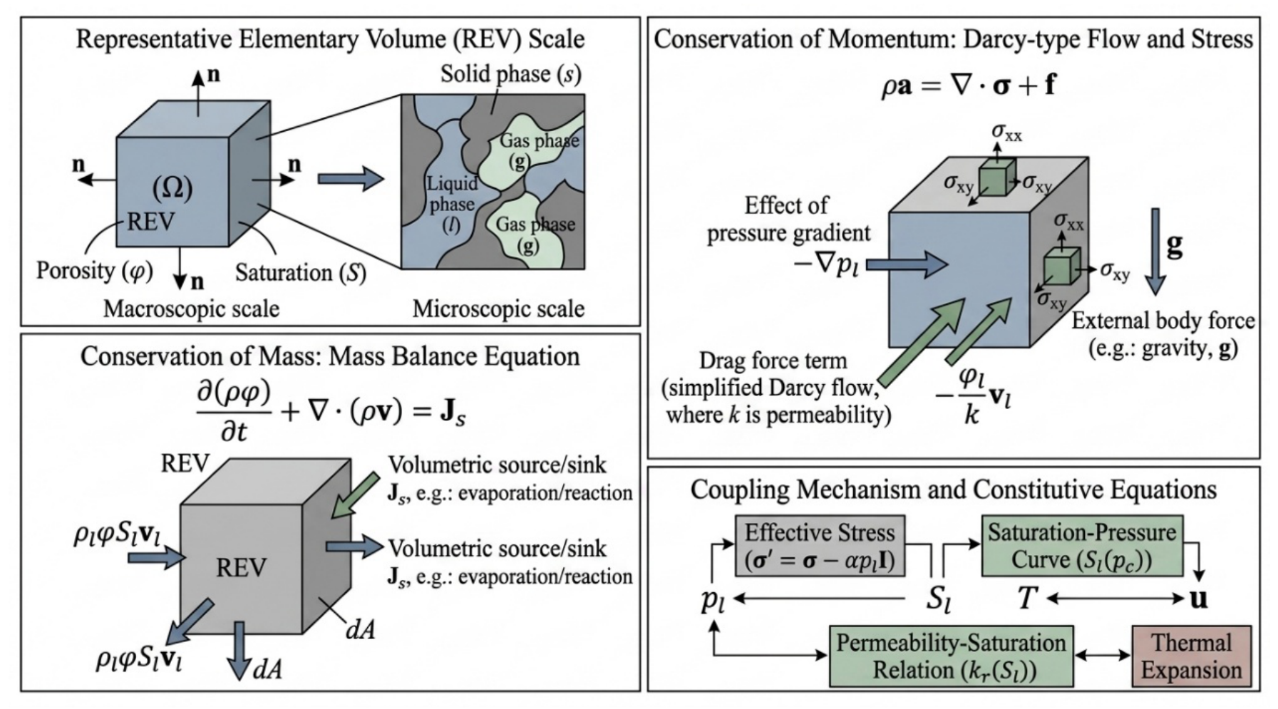
The representative-volume concept and its coupling relationships are illustrated in Figure 3.
The formulation is based on the following assumptions. Oil and water are slightly compressible and occupy the pore space, and their saturations sum to unity in each continuum. Matrix flow includes a threshold pressure gradient, whereas fracture flow follows Darcy’s law. The rock skeleton undergoes small, linear-elastic deformation, and mechanical equilibrium is quasi-static, following the poroelastic modelling tradition [3]. A local thermal equilibrium approximation assigns a common temperature to the matrix and fractures at the same location. Heat transport includes conduction and fluid advection; phase change, chemical reactions, and thermal radiation are outside the model scope. Porosity and permeability depend on effective stress through exponential constitutive relations.
Two exchange contributions are included: pressure-driven intercontinuum flow and an empirical imbibition term. The latter represents water uptake by the matrix and associated oil displacement at the continuum scale. These are modelling closures rather than explicit descriptions of pore-scale interfaces. The interpretation of both contributions depends on the adopted sign conventions, phase partitioning, and exchange-volume basis.
Figure 4.
Conceptual relationships among mass balance, momentum transfer, and constitutive properties. The phase definitions and governing equations used here are those stated in the text.
Figure 4.
Conceptual relationships among mass balance, momentum transfer, and constitutive properties. The phase definitions and governing equations used here are those stated in the text.
2.2. Phase Mass Balances and Flow Relations
Oil and water mass balances are written for both continua. The left-hand sides describe fluid accumulation and advective transport, whereas the right-hand sides contain well source or sink terms and intercontinuum exchange:
Here, denotes porosity, denotes phase density, S denotes saturation, and (or v in the heat-flux expressions) denotes Darcy velocity. The phase saturations satisfy and . The symbol q denotes a well source or sink, denotes pressure-driven exchange, and denotes the imbibition contribution. Exchange represents internal transfer between the two continua and must cancel in the combined mass balance when the continuum volume convention is applied consistently.
The porosity relations express the response to a change in effective stress:
The corresponding effective stress expressions are
where and are Biot coefficients and the subscript 0 denotes a reference state. Effective stress in an exponential scalar property law must be distinguished from the effective stress tensor used in mechanical equilibrium.
The density of each phase depends on pressure and temperature through the linearised relations
where C is fluid compressibility and is the thermal expansion coefficient. The pressure in each density relation refers to the corresponding continuum.
To represent low-gradient resistance in the matrix, we adopt the following threshold-gradient closure. Related pre-Darcy models account for stress sensitivity and nonlinear mobility [8,9]. Fracture flow is described by Darcy relations:
In these expressions, and are absolute permeabilities, is relative permeability, is dynamic viscosity, D is depth, and g is gravitational acceleration. The symbols and denote threshold pressure gradients in this equation. Relative permeability describes the reduction in phase mobility associated with the presence of the other phase. Because phase velocity appears in a unit-direction term, the zero-velocity limit requires a defined treatment in the numerical implementation.
2.3. Matrix–Fracture Exchange
Pressure-driven exchange is represented by a linear transfer relation:
The coefficient controls the exchange response to the pressure difference. With the direction defined in Equation (6), a positive value corresponds to transfer from fractures towards the matrix. An equal and opposite contribution enters the mass balance of the other continuum. Phase-specific exchange terms also require a consistent allocation between oil and water.
The empirical imbibition relation is
where J is the imbibition coefficient, L is a characteristic matrix-block length, is the saturation parameter used in the exchange closure, and is residual matrix oil saturation. The term describes water uptake and the associated oil exchange [11]. Its saturation dependence should be interpreted as the chosen constitutive approximation, rather than as a resolved capillary-pressure field. The meaning and units of the oil and water transfer rates must remain consistent with the phase mass balances.
2.4. Mechanical Response and Permeability Evolution
Mechanical response is represented by quasi-static equilibrium, neglecting inertia and plastic deformation:
For an idealised parallel-plate fracture, permeability is related to aperture by . Fracture conductivity is defined as , where is the width used in the conductivity relation. Conductivity therefore has units of permeability multiplied by length and is distinct from permeability alone.
Stress-dependent fracture permeability is expressed as [10]
The matrix permeability relation includes a matrix-specific stress response and a factor that accounts for its dependence on fracture conductivity:
The coupling factor is
where is the reference coupling parameter and is reference fracture conductivity. These relations describe permeability changes associated with the current effective stress. They do not, by themselves, establish irreversible damage or loading-unloading hysteresis. Accordingly, the results below are discussed in terms of stress-dependent permeability reduction rather than permanent degradation.
2.5. Thermal Relations and Temperature-Dependent Viscosity
The local thermal equilibrium approximation uses one temperature field for the co-located matrix and fracture continua. The thermal formulation includes energy storage, conduction through the porous medium, and advection by both fluid phases. The energy-storage expressions assigned to the two continua are
where is solid density and , , and are the specific heat capacities of the solid, oil, and water. These expressions require a consistent reference-volume convention when combined in an energy balance with a shared temperature.
The advective heat flux is expressed as
and Fourier conduction is described by
The effective thermal conductivities are
In Equations (14) and (15), denotes thermal conductivity; , , and refer to the solid and fluid phases. These thermal coefficients are distinct from the threshold pressure gradients denoted by and in Equation (5). This distinction must also be maintained in the implementation and symbol definitions.
Temperature-dependent viscosity is represented by an exponential relation [6]:
where is the viscosity of phase at the reference temperature and controls temperature sensitivity. The second-order approximation used in the formulation is
Equation (17) is a local expansion about . Its suitability depends on the magnitude of , rather than on temperature alone. The approximation is not assumed to be uniformly accurate over every temperature range considered in reservoir applications.
2.6. Coupling Interpretation
The relations above couple flow, mechanics, and temperature through explicit dependencies among material properties. Pressure influences effective stress; effective stress influences porosity and permeability; and temperature influences viscosity and density. Fluid motion contributes to heat transport, while exchange transfers fluid between continua. The resulting feedback is represented at the continuum scale. Individual fracture opening, fracture propagation, and pore-scale capillary interfaces are not resolved.
These dependencies describe the physical intent of the formulation. They also group the neural residuals by physical process, so that pressure, saturation, thermal transport, and stress-dependent properties can be considered within one training objective.
2.7. Constitutive Summary and Coupling Pathways
Table 1 and Table 2 summarise the property relations and coupling pathways. The separation of fluid properties, medium properties, and exchange terms makes the model structure easier to follow. Fracture conductance is related to aperture and permeability, consistent with the classical role of fracture geometry in hydraulic conductance [4].
3. Fourier-PINN Approximation and Training
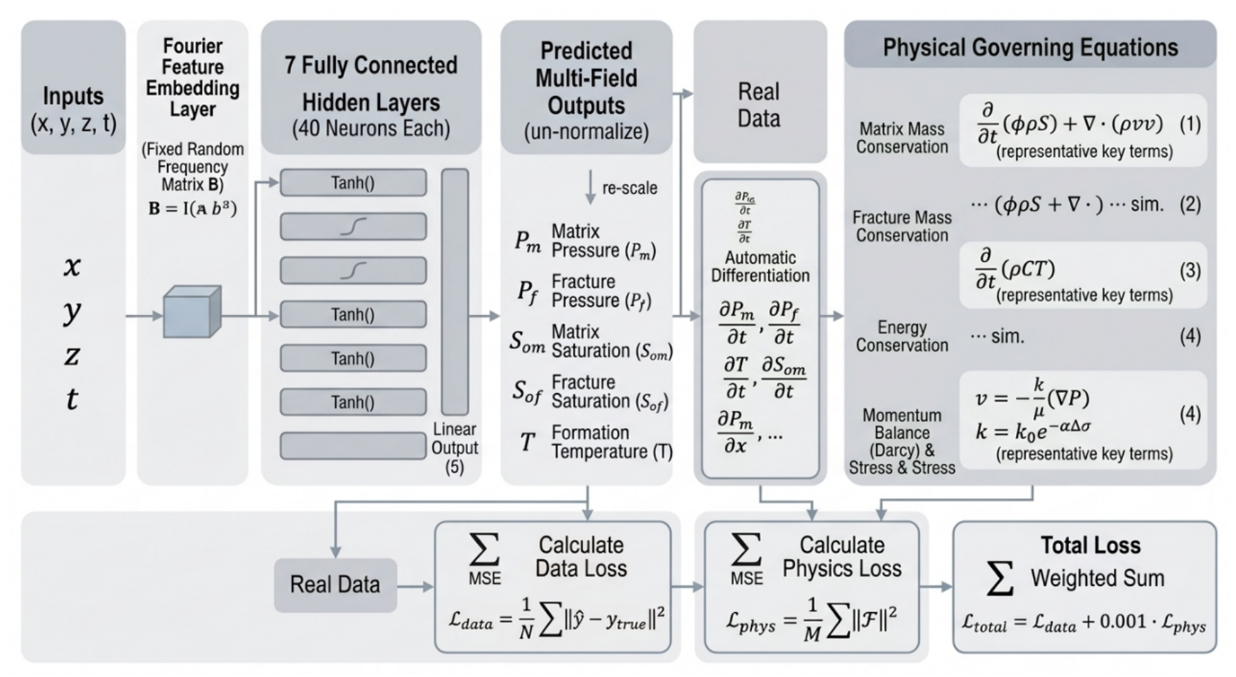
The solution framework combines a continuous neural approximation with the physical relations of Section 2. Figure 5 summarises how reservoir inputs, field interactions, and output quantities are connected. The data term constrains the approximation using reference values, while automatic differentiation supplies the derivatives used in the physical residuals.
3.1. Coordinate Mapping and Network Outputs
The Fourier-PINN takes the space-time coordinate vector as input and applies a fixed Fourier feature map before the fully connected network:
The matrix contains the frequencies used by the sine and cosine functions and is held fixed during training. This mapping enriches the input representation; it is not a Fourier transform of the computed solution. The approach follows established Fourier-feature representations [28,29], whose effectiveness depends on the frequencies selected for the problem.
The mapped inputs pass through seven hidden layers, each with 40 neurons and hyperbolic tangent activation functions. The linear output layer predicts five quantities: matrix pressure , fracture pressure , matrix oil saturation , fracture oil saturation , and temperature T. Water saturation in each continuum is calculated as one minus the oil saturation. The baseline PINN uses the same hidden-layer depth and width without the Fourier input map. Because the input dimension changes after mapping, equal hidden-layer sizes do not necessarily imply equal trainable parameter counts.
The five network outputs represent the primary learned fields. A mechanical residual additionally requires displacement or stress information, either obtained from supplementary variables or a defined closure. Mechanical-field accuracy cannot be inferred solely from the pressure, saturation, and temperature outputs.
Figure 6.
Fourier-PINN architecture and automatic-differentiation workflow. Numerical loss weights in the illustration are schematic; the settings used in this manuscript are specified in Table 3.
Figure 6.
Fourier-PINN architecture and automatic-differentiation workflow. Numerical loss weights in the illustration are schematic; the settings used in this manuscript are specified in Table 3.
3.2. Data and Physics Losses
Training minimises a weighted combination of reference-data error and physical residuals:
The weights and in Equation (19) correspond to and , respectively. Their reported initial values are 0.1 and 0.9. These coefficients express the relative emphasis of the two loss terms; they do not guarantee that every physical constraint is satisfied to the same accuracy.
The data loss is the mean squared difference between predictions and reference values at labelled points:
Here, is the predicted field vector, is the reference-data vector, and is the number of labelled samples. The subscript obs is retained as notation and does not establish whether the reference values originated from field measurements, laboratory observations, or numerical calculations.
The physics loss groups the mass, mechanical, thermal, and additional constraint residuals:
The residual represents the phase mass balances in the two continua. groups the mechanical and stress-dependent property relations, while represents thermal relations. represents additional exchange, constitutive, and initial or boundary constraints in the reported loss definition. denotes the number of physical collocation points. The magnitude of this aggregate loss depends on the residual definitions, units, and scaling; it is not a direct estimate of the error in the PDE solution.
3.3. Training Procedure and Reported Settings
Space-time coordinates and field variables are scaled using min-max normalisation. The labelled dataset is divided into training and test sets in a 9:1 ratio. Physical collocation points are sampled randomly and uniformly within the computational domain. The test-data comparison and the extrapolation assessment serve different purposes and should not be treated as interchangeable evidence of generalisation.
During training, the mapped coordinates are propagated through the network, and automatic differentiation supplies the derivatives needed to evaluate the residuals. Derivatives with respect to normalised coordinates must be related to physical-coordinate derivatives through the corresponding scale factors. The Adam optimiser updates the network parameters, with cosine annealing applied to the learning rate. Predictions are transformed back to physical units for analysis. Table 3 summarises the computational settings.
The stopping rule uses a change in total loss below 10-6 over 2000 consecutive iterations, with a maximum of 25,000 iterations. Loss values are recorded every 500 iterations. These settings describe the reported training procedure but do not establish a repeatability bound across random initialisations.
4. Numerical Assessment and Parameter Study
4.1. Benchmark Setup and Assessment Scope
The benchmark represents a low-permeability matrix coupled to a more permeable fracture continuum. Table 4 lists the reference properties. The study examines agreement with the reference dataset, training behaviour, field distributions, and responses to selected parameter changes. No comparison with an independently implemented finite-volume or finite-element solver, analytical solution, or manufactured solution is included in the present assessment.
The primary accuracy comparison uses the coefficient of determination, . A value close to unity indicates close agreement with the reference values under this metric, whereas a negative value indicates poorer performance than a constant prediction equal to their mean. The interpretation is conditional on the test set and does not establish the provenance or accuracy of the reference values themselves.
4.2. Agreement with Reference Data
Table 5 reports the values for the baseline PINN and Fourier-PINN. The value increases from 0.410 to 0.923 for matrix pressure, from 0.415 to 0.923 for matrix oil saturation, and from −1.7126 to 0.947 for temperature. These values support improved agreement for these three variables within the reported comparison.
Fracture pressure does not follow the same pattern: the tabulated decreases from 0.096 to 0.025. The reported results therefore do not support a claim that Fourier mapping improves every output or resolves the difficulties in predicting fracture pressure. Percentage improvements are not used because ratios of values can be misleading, particularly when the baseline is close to zero or negative.
Figure 7 presents the available prediction-reference scatter plots. These panels are treated as variable-wise diagnostics rather than a complete paired comparison of the two architectures. The labels in the pressure panels are not consistent with all of the Fourier-PINN entries in Table 5, so they do not provide independent confirmation of the pressure comparison. The aggregate evidence supports a qualified improvement for several variables while leaving fracture-pressure performance unresolved.
4.3. Residual Diagnostics and Predicted Fields
The residual summary reports mean physical residuals of order 10-5 and a saturation-constraint residual of order 10-6. These magnitudes characterise the stated residual calculation at sampled points. Their physical significance depends on the component definitions and normalisation, and they do not establish exact conservation throughout the domain. Moreover, when water saturation is computed as one minus oil saturation, the saturation sum is an algebraic constraint rather than an independent verification of phase mass conservation.
Figure 8, Figure 9 and Figure 10 present the predicted fields at 8, 9, and 10 days. The pressure, saturation, and temperature panels exhibit spatial variation, while the stress and permeability panels contain finer-scale structure. The figures display the network outputs and derived quantities; visual continuity alone cannot determine whether the spatial scales or amplitudes are physically accurate. In particular, the displayed stress and permeability variations require separate assessment before they can be interpreted as resolved physical heterogeneity.
4.4. Training Behaviour and Reported Extrapolation
The Fourier-PINN training history in Figure 11 shows a reduction in the total and data losses over the plotted iterations. The physics loss contains substantial fluctuations. This behaviour indicates progress in optimisation, but does not support a claim of uniformly smooth convergence. As the figure does not include a baseline-PINN curve, it also does not establish a difference in convergence rate or a reduction in wall-clock time.
The reported average relative errors in an extrapolation test are 14.7% for the baseline PINN and 4.2% for the Fourier-PINN. These values suggest improved performance in that particular test. Their interpretation nevertheless depends on the withheld space-time region, the reference values, and the error-aggregation rule. Without those details and repeated trials, they do not establish reliable long-term forecasting or transfer to new reservoir configurations. A network conditioned only on space and time is not automatically a parameter-conditioned surrogate for unseen development scenarios.
4.5. Parameter Variations
The parameter study varies one selected input at a time while holding the other benchmark settings fixed. Table 6 summarises the reported cases. The values expressed in mD correspond to fracture permeability, , rather than fracture conductivity, . At fixed fracture width, changing also changes conductivity proportionally.
The scenario design is summarised in Figure 12, connecting controlled parameter variations to field and coupling diagnostics.
4.5.1. Pressure Communication
The scenario descriptions associate higher fracture permeability with faster pressure communication through the fracture continuum and a smaller matrix-fracture pressure difference. Increasing matrix permeability is reported to have a weaker effect on the pressure response over the examined ranges. Higher temperature reduces viscosity through the adopted constitutive law, while stronger stress sensitivity reduces permeability as effective stress rises. Increasing the exchange coefficient accelerates communication between the continua.
These trends are consistent with the roles assigned to permeability, viscosity, and exchange in the formulation. They are interpreted as responses within the selected cases, rather than as a universal ordering of parameter influence. Quantitative comparisons of front speed or equilibration time would require explicitly defined response measures and corresponding scenario data.
4.5.2. Saturation Response
The scenario descriptions suggest that fracture and matrix permeability, together with intercontinuum exchange, influence the redistribution of oil and water. Greater matrix mobility or stronger exchange can support transfer of matrix oil to the fracture continuum under favourable pressure and saturation conditions. Stress-dependent permeability reduction can restrict that transfer as production proceeds.
Saturation changes alone do not establish improved sweep efficiency, delayed water breakthrough, or a higher ultimate recovery factor. Those outcomes also depend on boundary conditions, injection and production controls, and the spatial distribution of the flow paths. Accordingly, the present results are used to discuss oil mobilisation tendencies rather than to prescribe an optimal development strategy.
4.5.3. Thermal and Mechanical Effects
The adopted viscosity relation links changes in temperature to phase mobility, while fluid velocities enter the advective heat flux. Pressure changes alter effective stress and therefore the permeability coefficients. These dependencies explain how thermal and mechanical conditions can modify the predicted flow response.
The effective-stress constitutive laws describe a decrease in permeability as the corresponding stress measure increases. The magnitude of this response depends on the selected sensitivity coefficients. The current evidence does not establish irreversible fracture closure, long-term material damage, or a general increase in recovery from thermal intervention.
4.6. Qualitative Ordering of Parameter Influence
Table 7 presents the reported ranking of six parameters. The categories are qualitative; no numerical sensitivity index, uncertainty interval, or normalised response coefficient accompanies them. This ordering also concerns a parameter set that is not identical to the five variation groups in Table 6. It is therefore presented as an exploratory interpretation rather than a quantitative global sensitivity analysis.
The two highest-ranked parameters identify fracture permeability and matrix-fracture exchange as priorities for further examination within the stated benchmark. The ordering should not be transferred to reservoirs with different geometries, property distributions, operating conditions, or parameter ranges without additional assessment. Figure 13 provides a graphical view of the ordering in Table 7.
5. Discussion
5.1. An Integrated Representation of Coupled Reservoir Processes
The central contribution of this study is a unified modelling framework for oil-water transport in interacting matrix and fracture continua. Separate pressure and saturation fields represent their contrasting storage and transport roles, while exchange terms connect the two environments. Stress-sensitive porosity and permeability and temperature-dependent fluid properties embed the principal THM feedbacks in the same formulation. This formulation allows the reservoir response to be interpreted in terms of the underlying physical dependencies.
A particular strength of the dual-continuum representation is the separation of transport capacity from fluid supply. Fractures provide conductive pathways, but the matrix stores a substantial part of the fluid and supplies those pathways through exchange. Representing both contributions explicitly helps explain why a change in fracture permeability and a change in exchange intensity can have different consequences for pressure communication and saturation redistribution. The pressure-driven and imbibition-related terms also retain two complementary mechanisms of matrix-fracture interaction.
The formulation further links reservoir properties to the evolving state. A pressure decline changes effective stress and hence permeability, whereas temperature modifies viscosity and phase mobility. Consequently, pressure, saturation, and temperature are considered as interacting fields rather than separate indicators. This provides a physically grounded basis for interpreting the time-dependent results and the parameter study.
5.2. Benefits of Fourier-Feature Physics-Informed Approximation
Fourier mapping introduces sinusoidal coordinate features before the fully connected network. These features enrich the representation of spatial and temporal variation and are well suited to the coexistence of different characteristic scales in the matrix and fracture responses [28,29]. The present contribution is their integration with the oil-water dual-continuum THM formulation and its data-and-physics training objective.
The benchmark results show the clearest benefits for matrix pressure, matrix oil saturation, and temperature. The corresponding reported values increase from to , from to , and from to , respectively. These improvements indicate that the evaluated representation captures useful information about both the flow state and its thermal environment. The performance benefit is variable-dependent, as shown by the fracture-pressure values in Table 5.
The hybrid loss provides a common optimisation framework for labelled data and physical relations. Automatic differentiation evaluates the derivatives of the neural approximation for the physical residuals. The residual diagnostics and the reduction in the reported extrapolation error, from 14.7% to 4.2%, complement the comparisons for individual variables. Together, these observations support the utility of the combined approach for the benchmark considered here.
Once trained, the coordinate-based network can evaluate the primary fields at requested space-time locations. This continuous representation supports consistent visualisation of pressure, saturation, and temperature without a separate interpolation model for each quantity. The corresponding derived fields can then be interpreted through the same constitutive relationships used to formulate the physical problem.
5.3. Reservoir Insights from the Parameter Study
The parameter study identifies fracture permeability and intercontinuum exchange as influential controls within the examined benchmark. Higher fracture permeability promotes pressure transmission along the conductive continuum, whereas a stronger exchange coefficient facilitates communication with matrix storage. Considering both parameters together provides a more informative description of reservoir mobilisation than considering fracture transport capacity in isolation.
The saturation response extends this interpretation. Matrix permeability influences the ability of stored oil to move, and exchange determines how that mobilisation couples to fracture flow. Temperature and stress sensitivity modify the mobilities through viscosity and permeability, respectively. The results therefore suggest an interaction between transport pathways, matrix supply, and state-dependent properties: the effect of a change in one component depends on the conditions in the others.
The thermal and mechanical relations also clarify competing tendencies during production. A temperature increase reduces viscosity under the adopted law and thereby promotes mobility. An increase in effective stress reduces permeability under the stress-sensitive constitutive relations and can restrict pressure communication. Their joint representation is useful for examining how thermal conditions and pressure evolution influence the same flow process.
For reservoir characterisation, these observations suggest a practical order of priority for examining the model parameters. Fracture transport properties and matrix-fracture exchange deserve particular attention, followed by the thermal and stress-dependent property responses that modulate them. The qualitative ranking applies to the selected conditions and provides a structured interpretation of the scenario results.
5.4. Modelling Value and Application Scope
The framework connects physical formulation, neural training, field diagnostics, and controlled parameter comparisons in a single workflow. Its value lies in linking these components for physical interpretation: changes in a constitutive parameter can be related to a physical mechanism and then examined through the predicted fields. The conceptual diagrams and field visualisations make this connection explicit across the manuscript.
The conclusions apply to the stated dual-continuum assumptions, reference comparisons, and parameter ranges. Within that scope, the study offers a coherent basis for analysing coupled oil-water reservoir behaviour and for developing physics-informed computational tools that combine physical structure with continuous field approximation.
6. Conclusions
This study presents a Fourier-feature physics-informed neural network for thermo-hydro-mechanical modelling of oil-water flow in fractured porous media represented by two interacting continua. The physical formulation and the neural approximation are connected through a hybrid training objective. The principal conclusions are as follows.
- 1.
- The coupled model brings phase mass balances, mechanical equilibrium, thermal relations, stress-sensitive properties, and matrix-fracture exchange into a common framework. Separate matrix and fracture variables retain their different storage and transport roles, while pressure-driven transfer and imbibition connect their responses.
- 2.
- The Fourier-PINN improves the reported agreement with the reference data for matrix pressure, matrix oil saturation, and temperature, with values of 0.923, 0.923, and 0.947, respectively. The comparisons demonstrate the benefit of the evaluated Fourier-feature configuration for these coupled fields under the benchmark conditions.
- 3.
- The data-and-physics objective and automatic differentiation provide an integrated training procedure. The reported extrapolation comparison gives an average relative error of 4.2% for the Fourier-PINN, compared with 14.7% for the baseline PINN, supporting its usefulness in this test.
- 4.
- The scenario analysis highlights fracture permeability and matrix-fracture exchange as major influences on pressure communication and oil mobilisation. Temperature-dependent viscosity and stress-sensitive permeability further regulate the response, emphasising the importance of retaining thermal and mechanical feedbacks in oil-water flow modelling.
Overall, the study provides an integrated and interpretable approach to coupled reservoir modelling. By combining a structured physical description with continuous neural field approximation, it supports analysis of the relationships among fracture transport, matrix supply, and evolving reservoir properties within the investigated conditions.
Author Contributions
Conceptualization, methodology, formal analysis, investigation, validation, visualization, and writing—original draft preparation, Y.Z., C.Z. and J.T.; writing—review and editing and supervision, L.W., Q.Z., X.L. and L.K. All authors have read and agreed to the published version of the manuscript.
Funding
This research received no external funding.
Data Availability Statement
Data supporting the findings of this study are presented in this article. Additional supporting data can be obtained by contacting the corresponding author.
Conflicts of Interest
The authors declare no conflicts of interest.
Appendix A. Nomenclature
Subscripts m and f identify the matrix and fracture continua; o and w identify oil and water. The subscript 0 denotes the relevant reference state. The tables list physical quantities and learning variables separately. Benchmark values are given in Table 4 rather than mixed with illustrative ranges.

Table A1.
Physical quantities and notation.
| Symbol | Meaning | Unit or convention |
|---|---|---|
| m, f; o, w | Matrix, fracture; oil, water | Subscripts |
| 0 | Reference state | Subscript |
| , | Matrix and fracture porosities | Dimensionless |
| , , | Oil, water, and solid densities | kg m-3 |
| , | Densities in mechanical body-force terms | kg m-3; volume basis to specify |
| , | Oil saturation in matrix and fractures | Dimensionless |
| , | Water saturation in matrix and fractures | Dimensionless |
| Saturation parameter in Equation (7) | Dimensionless; closure-specific | |
| Residual matrix oil saturation | Dimensionless | |
| x, y, z; t | Spatial coordinates; time | m; s (figures may use days) |
| ∇; ∇· | Gradient; divergence | Differential operators |
| , , , | Phase Darcy velocities (also written v in heat flux) | m s-1 |
| , , , | Phase-specific well source or sink terms | Mass per reference volume per time |
| , | Pressure-driven phase exchange | Same basis as the phase mass balance |
| , | Imbibition-related phase exchange | Same basis as the phase mass balance |
| , | Exchange coefficient notation | Units set by Equation (6) and q basis |
| J | Imbibition coefficient | kg m-2 s-1 under stated mass-rate convention |
| L | Characteristic matrix-block length | m |
| , ; , | Current and reference permeability | mD in parameter tables |
| , , , | Phase relative permeabilities | Dimensionless |
| , ; | Dynamic viscosity; reference viscosity | mPa s in original parameter convention |
| , ; | Continuum pressures; reference pressure | MPa in parameter tables |
| D; g | Depth; gravitational acceleration | m; m s-2 |
| , in Equation (5) | Phase threshold pressure gradients | MPa m-1 |
| ; | Total and effective stress | MPa |
| , | Effective stress measures for property laws | MPa; scalar definition required |
| , | Biot coefficients | Dimensionless |
| , | Permeability stress-sensitivity coefficients | MPa-1 |
| , | Porosity stress-sensitivity coefficients | MPa-1 |
| , | Fluid compressibility coefficients | MPa-1 with pressure in MPa |
| , | Fluid thermal expansion coefficients | K-1 |
| C in Table 7 | Rock compressibility coefficient | Pressure-1; convention to specify |
| u; | Displacement; strain tensor | m; dimensionless |
| I; | Identity tensor; Kronecker delta | Dimensionless |
| Linear thermal expansion coefficient | K-1 | |
| T; | Temperature; reference temperature | in parameter tables |
| , , | Solid and fluid specific heat capacities | J kg-1 K-1 |
| , | Continuum energy-storage quantities | J per adopted reference volume |
| , | Advective and conductive heat flux | W m-2 |
| , , | Effective thermal conductivities | W m-1 K-1 |
| , , in Equation (15) | Solid and phase thermal conductivities | W m-1 K-1 |
| Viscosity temperature-sensitivity coefficient | K-1 | |
| , | Fracture aperture and conductivity width | m |
| , | Current and reference fracture conductivity | mD m |
| , | Conductivity coupling factor and parameter | Dimensionless |
Units must be converted consistently before residual evaluation. A temperature difference of 1 equals 1 K. The transfer-rate and energy-volume conventions require an explicit implementation definition.
Table A2.
Network and loss notation.
| Symbol | Meaning |
|---|---|
| x; | Space-time coordinate vector; Fourier feature map |
| B | Fixed random frequency matrix |
| ; | Predicted field vector; reference-data vector |
| ; | Number of labelled samples; number of physical collocation points |
| ; ; | Data loss; physics loss; total loss |
| , ; , | Data and physics weights in Equation (19) |
| ; ; ; | Residual groups defined in Equation (21) |
| Coefficient of determination |
References
- Warren, J.E.; Root, P.J. The Behavior of Naturally Fractured Reservoirs. Soc. Pet. Eng. J. 1963, 3, 245–255. [Google Scholar] [CrossRef]
- Snow, D.T. Anisotropic permeability of fractured media. Water Resour. Res. 1969, 5, 1273–1289. [Google Scholar] [CrossRef]
- Biot, M.A. General Theory of Three-Dimensional Consolidation. J. Appl. Phys. 1941, 12, 155–164. [Google Scholar] [CrossRef]
- Witherspoon, P.A.; Wang, J.S.Y.; Iwai, K.; Gale, J.E. Validity of Cubic Law for fluid flow in a deformable rock fracture. Water Resour. Res. 1980, 16, 1016–1024. [Google Scholar] [CrossRef]
- Vaezi, I.; Yoshioka, K.; De Simone, S.; Gómez-Castro, B.M.; Paluszny, A.; Jalali, M.; Berre, I.; Rutqvist, J.; Min, K.B.; Lei, Q.; et al. A review of thermo-hydro-mechanical modeling of coupled processes in fractured rock: From continuum to discontinuum perspective. J. Rock Mech. Geotech. Eng. 2025, 17, 7460–7488. [Google Scholar] [CrossRef]
- Xu, F.; Li, Y.; Xu, X.; Yang, J.; Xiao, F.; Shi, Y. Thermal-hydrological-mechanical coupling simulation of matrix-type shale oil: Analysis of oil-gas-water multiphase flow mechanism under various parameter conditions. Geoenergy Sci. Eng. 2025, 246, 213656. [Google Scholar] [CrossRef]
- Lee, S.; Wheeler, M.F.; Wick, T. A phase-field diffraction model for thermo-hydro-mechanical propagating fractures. Int. J. Heat Mass Transf. 2025, 239, 126487. [Google Scholar] [CrossRef]
- Cheng, H.; Wang, F.; Guan, X.; Yang, G.; Yuan, Y.; Feng, G. A mathematical model for pre-Darcy flow in low permeability porous media with stress sensitivity and the boundary-layer effect. Eng. Geol. 2023, 324, 107257. [Google Scholar] [CrossRef]
- Cheng, H.; Wang, F.; Li, S.; Cheng, Z.; Yuan, Y.; Feng, G. From Pre-Darcy Flow to Darcy Flow in Porous Media: A Simple Unified Model. Water Resour. Res. 2024, 60, e2023WR036902. [Google Scholar] [CrossRef]
- Yang, H.; Cai, Z.; Zhang, H.; Sun, C.; Li, J.; Meng, X.; Liu, C.; Yang, C. Study on the Fluid-Solid Coupling Seepage of the Deep Tight Reservoir Based on 3D Digital Core Modeling. Energy Eng. 2025, 122, 537–560. [Google Scholar] [CrossRef]
- Hatiboglu, C.U.; Babadagli, T. Oil recovery by counter-current spontaneous imbibition: Effects of matrix shape factor, gravity, IFT, oil viscosity, wettability, and rock type. J. Pet. Sci. Eng. 2007, 59, 106–122. [Google Scholar] [CrossRef]
- Gimenez, J.M.; Idelsohn, S.R.; Oñate, E. Modeling and simulation of multiphase flow in highly fractured porous media with a data-driven multiscale approach. Comput. Mech. 2025, 75, 1847–1866. [Google Scholar] [CrossRef]
- Wen, G.; Li, Z.; Azizzadenesheli, K.; Anandkumar, A.; Benson, S.M. U-FNO—An enhanced Fourier neural operator-based deep-learning model for multiphase flow. Adv. Water Resour. 2022, 163, 104180. [Google Scholar] [CrossRef]
- Jiang, J. Simulating multiphase flow in fractured media with graph neural networks. Phys. Fluids 2024, 36, 023115. [Google Scholar] [CrossRef]
- Chen, J.; Yu, H.; Li, B.; Zhang, H.; Jin, X.; Meng, S.; Liu, H.; Wu, H. DeepONet-embedded physics-informed neural network for production prediction of multiscale shale matrix–fracture system. Phys. Fluids 2025, 37, 016608. [Google Scholar] [CrossRef]
- Raissi, M.; Perdikaris, P.; Karniadakis, G.E. Physics-informed neural networks: A deep learning framework for solving forward and inverse problems involving nonlinear partial differential equations. J. Comput. Phys. 2019, 378, 686–707. [Google Scholar] [CrossRef]
- Karniadakis, G.E.; Kevrekidis, I.G.; Lu, L.; Perdikaris, P.; Wang, S.; Yang, L. Physics-informed machine learning. Nat. Rev. Phys. 2021, 3, 422–440. [Google Scholar] [CrossRef]
- Samarkanov, O.L.; Riazi, M.; Irawan, S.; Kamrava, S. Applications of physics-informed neural networks in fluid flow in porous media - A review study. Energy AI 2026, 24, 100747. [Google Scholar] [CrossRef]
- Yan, X.; Lin, J.; Wang, S.; Zhang, Z.; Liu, P.; Sun, S.; Yao, J.; Zhang, K. Physics-informed neural network simulation of two-phase flow in heterogeneous and fractured porous media. Adv. Water Resour. 2024, 189, 104731. [Google Scholar] [CrossRef]
- Wang, C.; Guo, H.; Yan, X.; Shi, Z.L.; Yang, Y. Improved physics-informed neural networks for the reinterpreted discrete fracture model. J. Comput. Phys. 2025, 520, 113491. [Google Scholar] [CrossRef]
- Lin, J.Q.; Yan, X.; Wang, E.Z.; Zhang, Q.; Zhang, K.; Liu, P.Y.; Zhang, L.M. A layer-specific constraint-based enriched physics-informed neural network for solving two-phase flow problems in heterogeneous porous media. Pet. Sci. 2025, 22, 4714–4735. [Google Scholar] [CrossRef]
- Zhu, H.; Chen, Z.; Gao, X.; Chen, X.; Yu, W.; Sepehrnoori, K. A Physics-Informed Adaptive-Wavelet Neural Network (PIAWNN) for reservoir simulation with two-phase flow. Adv. Water Resour. 2026, 207, 105174. [Google Scholar] [CrossRef]
- Zhang, J.; Braga-Neto, U.; Gildin, E. Physics-Informed Neural Networks for Multiphase Flow in Porous Media Considering Dual Shocks and Interphase Solubility. Energy Fuels 2024, 38, 17781–17795. [Google Scholar] [CrossRef]
- Amini, D.; Haghighat, E.; Juanes, R. Physics-Informed Neural Network Solution of Thermo–Hydro–Mechanical Processes in Porous Media. J. Eng. Mech. 2022, 148, 04022070. [Google Scholar] [CrossRef]
- Amini, D.; Haghighat, E.; Juanes, R. Inverse modeling of nonisothermal multiphase poromechanics using physics-informed neural networks. J. Comput. Phys. 2023, 490, 112323. [Google Scholar] [CrossRef]
- Hu, H.; Qi, L.; Chao, X. Physics-informed Neural Networks (PINN) for computational solid mechanics: Numerical frameworks and applications. Thin-Walled Struct. 2024, 205, 112495. [Google Scholar] [CrossRef]
- Berardi, M.; Difonzo, F.V.; Icardi, M. Inverse Physics-Informed Neural Networks for transport models in porous materials. Comput. Methods Appl. Mech. Eng. 2025, 435, 117628. [Google Scholar] [CrossRef]
- Tancik, M.; Srinivasan, P.P.; Mildenhall, B.; Fridovich-Keil, S.; Raghavan, N.; Singhal, U.; Ramamoorthi, R.; Barron, J.T.; Ng, R. Fourier Features Let Networks Learn High Frequency Functions in Low Dimensional Domains. Proc. Adv. Neural Inf. Process. Syst. 2020, Vol. 33, 7537–7547. [Google Scholar]
- Wang, S.; Wang, H.; Perdikaris, P. On the eigenvector bias of Fourier feature networks: From regression to solving multi-scale PDEs with physics-informed neural networks. Comput. Methods Appl. Mech. Eng. 2021, 384, 113938. [Google Scholar] [CrossRef]
- Dolean, V.; Heinlein, A.; Mishra, S.; Moseley, B. Multilevel domain decomposition-based architectures for physics-informed neural networks. Comput. Methods Appl. Mech. Eng. 2024, 429, 117116. [Google Scholar] [CrossRef]
- Wang, S.; Li, B.; Chen, Y.; Perdikaris, P. PirateNets: Physics-informed Deep Learning with Residual Adaptive Networks. J. Mach. Learn. Res. 2024, 25, 1–51. [Google Scholar]
- Wang, S.; Teng, Y.; Perdikaris, P. Understanding and Mitigating Gradient Flow Pathologies in Physics-Informed Neural Networks. SIAM J. Sci. Comput. 2021, 43, A3055–A3081. [Google Scholar] [CrossRef]
- Wu, C.; Zhu, M.; Tan, Q.; Kartha, Y.; Lu, L. A comprehensive study of non-adaptive and residual-based adaptive sampling for physics-informed neural networks. Comput. Methods Appl. Mech. Eng. 2023, 403, 115671. [Google Scholar] [CrossRef]
- Anagnostopoulos, S.J.; Toscano, J.D.; Stergiopulos, N.; Karniadakis, G.E. Residual-based attention in physics-informed neural networks. Comput. Methods Appl. Mech. Eng. 2024, 421, 116805. [Google Scholar] [CrossRef]
- Wang, S.; Sankaran, S.; Perdikaris, P. Respecting causality for training physics-informed neural networks. Comput. Methods Appl. Mech. Eng. 2024, 421, 116813. [Google Scholar] [CrossRef]
- Chen, W.; Howard, A.A.; Stinis, P. Self-adaptive weights based on balanced residual decay rate for physics-informed neural networks and deep operator networks. J. Comput. Phys. 2025, 542, 114226. [Google Scholar] [CrossRef]
Figure 1.
Fractured-reservoir flow pathways and thermo-hydro-mechanical feedbacks motivating the coupled modelling framework.
Figure 1.
Fractured-reservoir flow pathways and thermo-hydro-mechanical feedbacks motivating the coupled modelling framework.
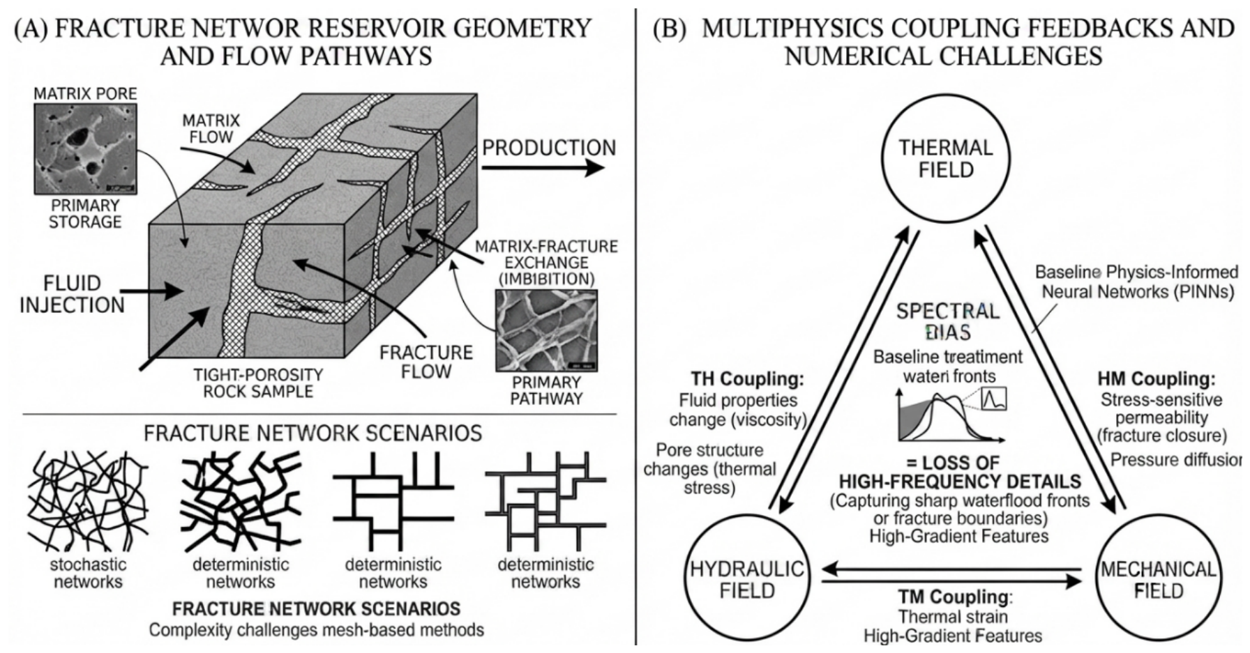
Figure 2.
Overview of the modelling and analysis workflow. The data-source boxes illustrate possible reference sources; the present comparisons use the reference data described in Section 3.
Figure 2.
Overview of the modelling and analysis workflow. The data-source boxes illustrate possible reference sources; the present comparisons use the reference data described in Section 3.
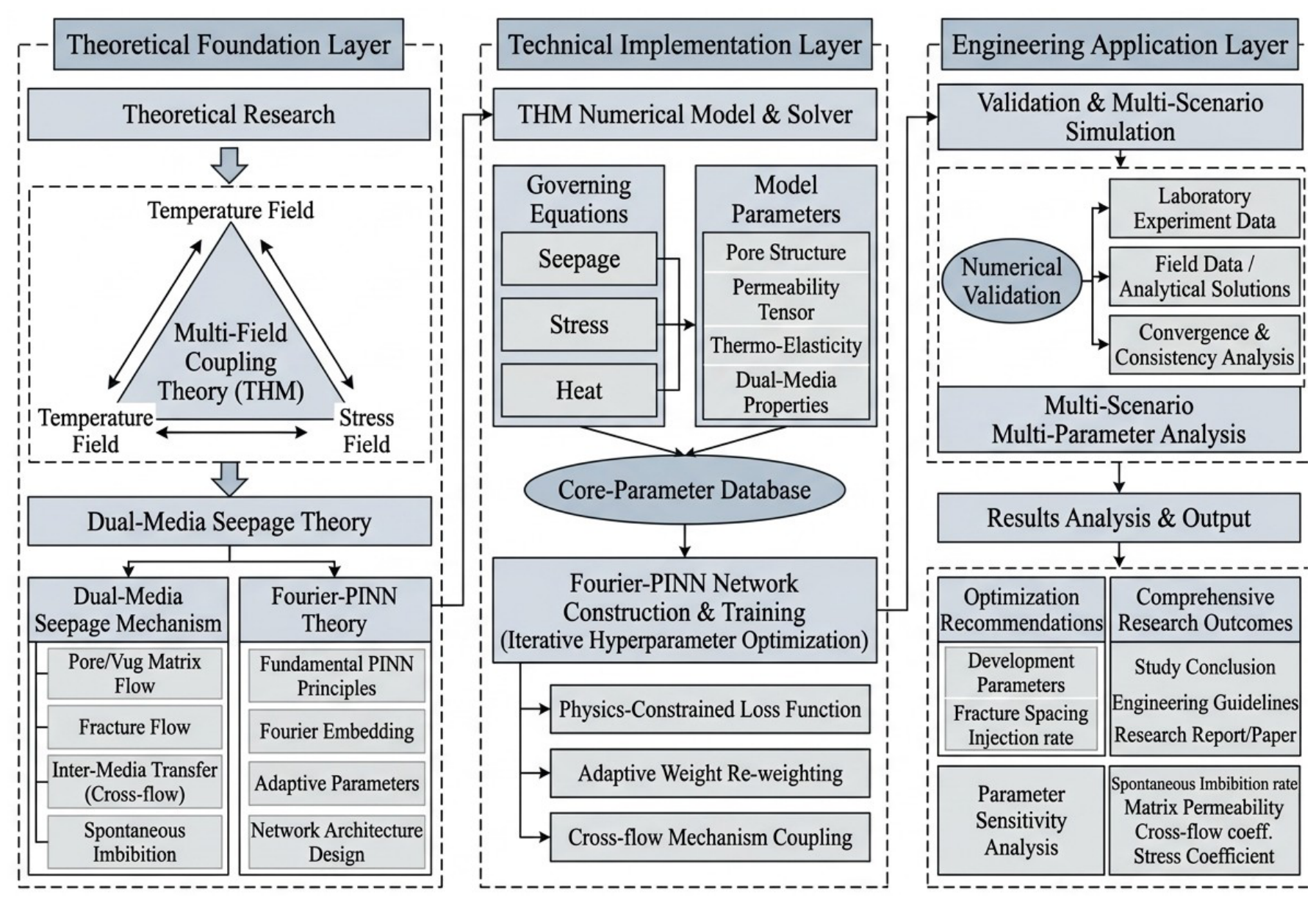
Figure 3.
Representative-volume view of interacting matrix and fracture continua. The generic multiphase symbols in the conceptual illustration are specialised to oil and water in the present formulation.
Figure 3.
Representative-volume view of interacting matrix and fracture continua. The generic multiphase symbols in the conceptual illustration are specialised to oil and water in the present formulation.
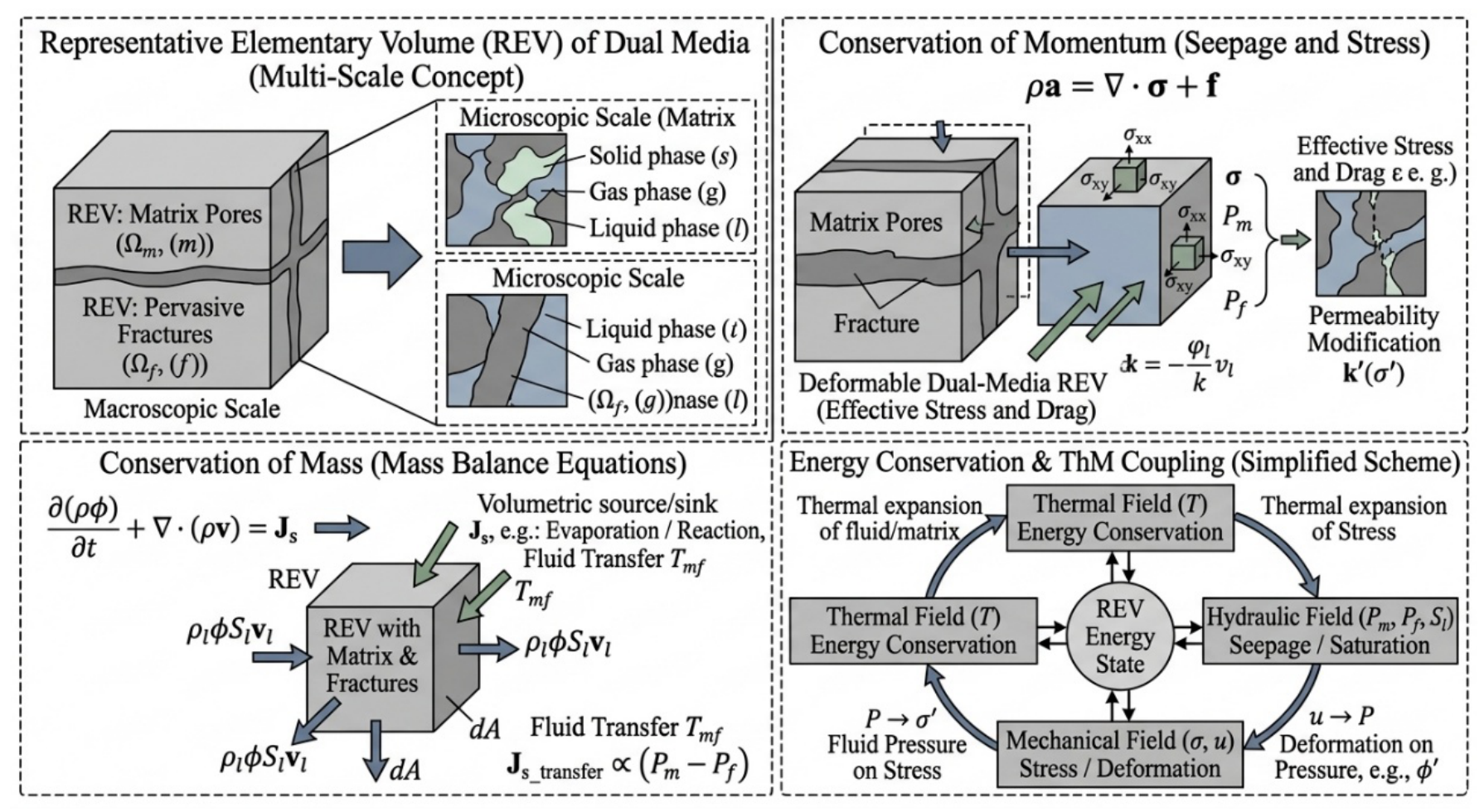
Figure 5.
Physics-informed modelling framework linking reservoir inputs, THM interactions, and predicted fields.
Figure 5.
Physics-informed modelling framework linking reservoir inputs, THM interactions, and predicted fields.
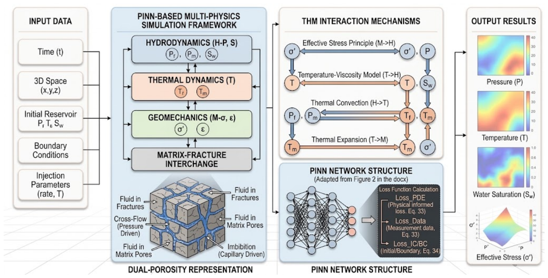
Figure 7.
Prediction-reference scatter plots for matrix pressure, fracture pressure, temperature, and oil saturation in the two continua. The panels are not a complete paired comparison of both networks; their pressure metrics require reconciliation with Table 5.
Figure 7.
Prediction-reference scatter plots for matrix pressure, fracture pressure, temperature, and oil saturation in the two continua. The panels are not a complete paired comparison of both networks; their pressure metrics require reconciliation with Table 5.
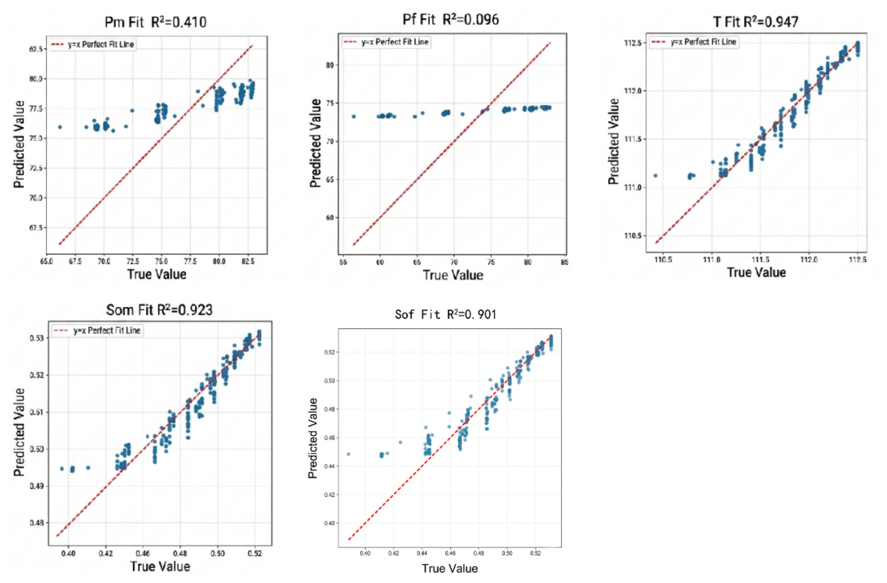
Figure 8.
Predicted pressure, saturation, temperature, effective stress, and permeability fields at 8 days. Colour scales are panel-specific; the plots show spatial outputs rather than independent solution verification.
Figure 8.
Predicted pressure, saturation, temperature, effective stress, and permeability fields at 8 days. Colour scales are panel-specific; the plots show spatial outputs rather than independent solution verification.
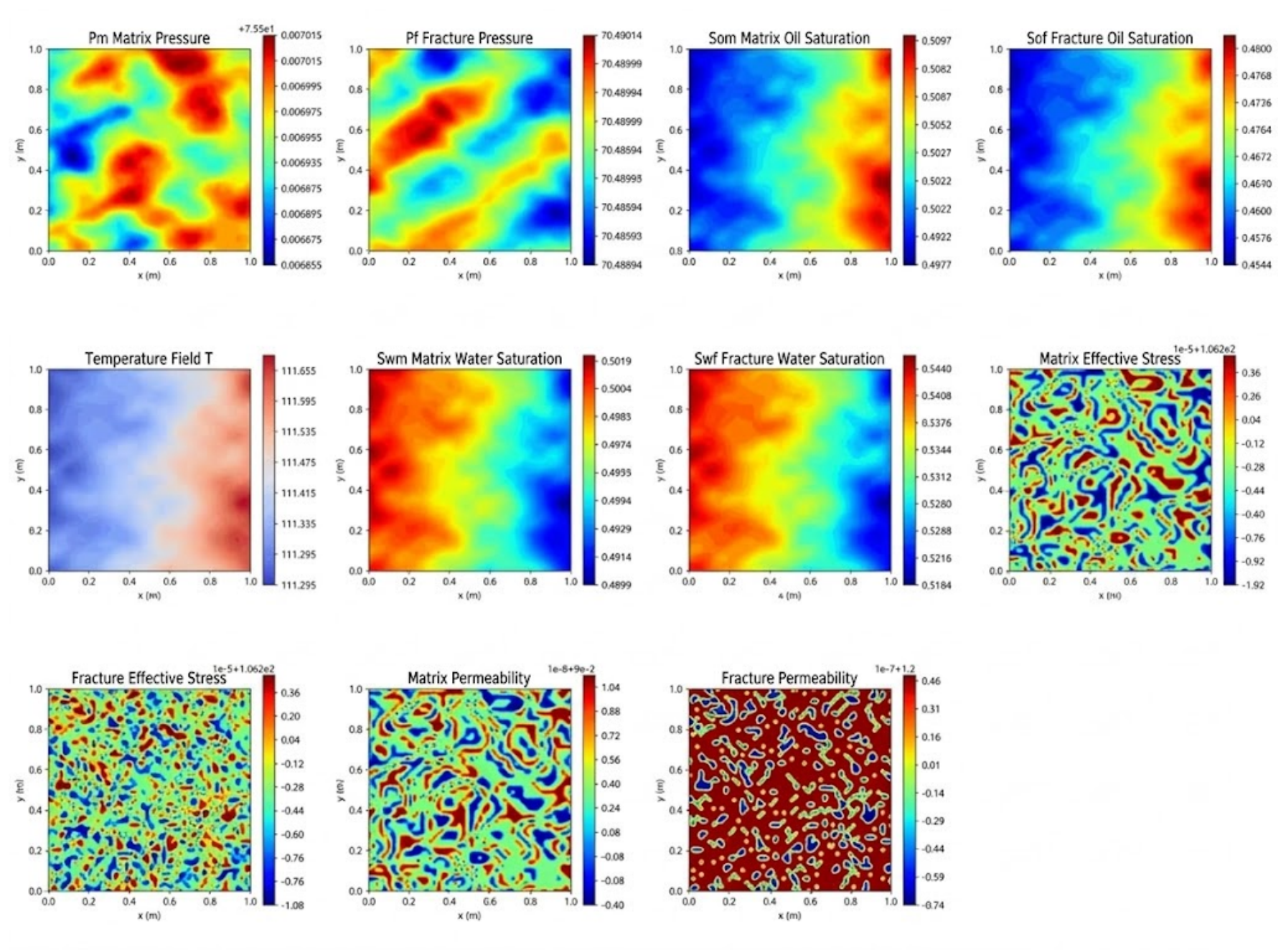
Figure 9.
Predicted fields at 9 days, with the same field ordering as Figure 8. Differences between panels and times should be interpreted together with their individual colour scales.
Figure 9.
Predicted fields at 9 days, with the same field ordering as Figure 8. Differences between panels and times should be interpreted together with their individual colour scales.
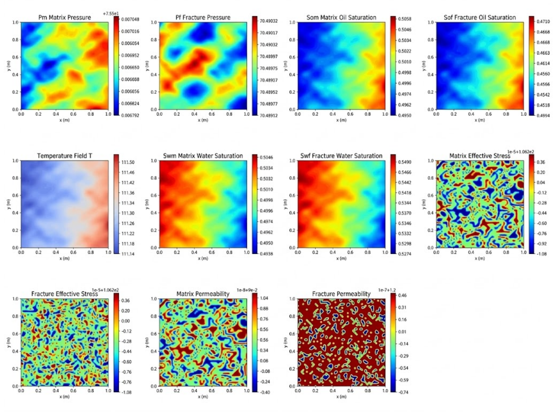
Figure 10.
Predicted fields at 10 days, with the same field ordering as Figure 8. These outputs are conditional on the adopted continuum formulation and benchmark setup.
Figure 10.
Predicted fields at 10 days, with the same field ordering as Figure 8. These outputs are conditional on the adopted continuum formulation and benchmark setup.
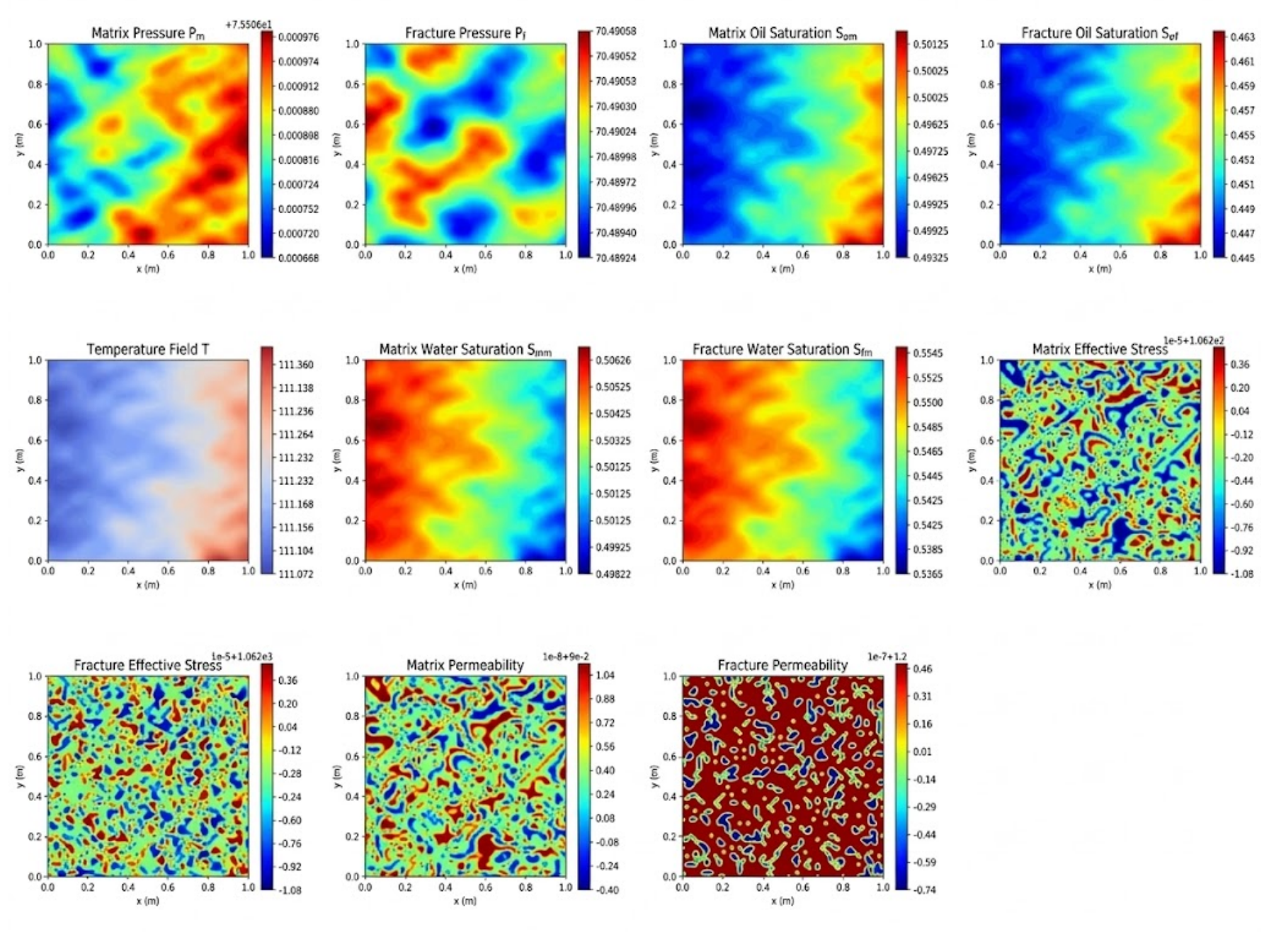
Figure 11.
Fourier-PINN training history. Total and physics losses use the left logarithmic axis, while data loss uses the right axis. The distinct scales must be considered when comparing the curves.
Figure 11.
Fourier-PINN training history. Total and physics losses use the left logarithmic axis, while data loss uses the right axis. The distinct scales must be considered when comparing the curves.
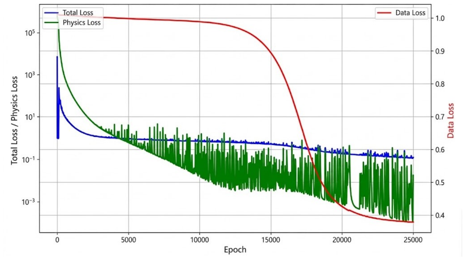
Figure 12.
Framework for the five groups of parameter variations. The mD values denote fracture permeability; conductivity varies proportionally when fracture width is fixed.
Figure 12.
Framework for the five groups of parameter variations. The mD values denote fracture permeability; conductivity varies proportionally when fracture width is fixed.
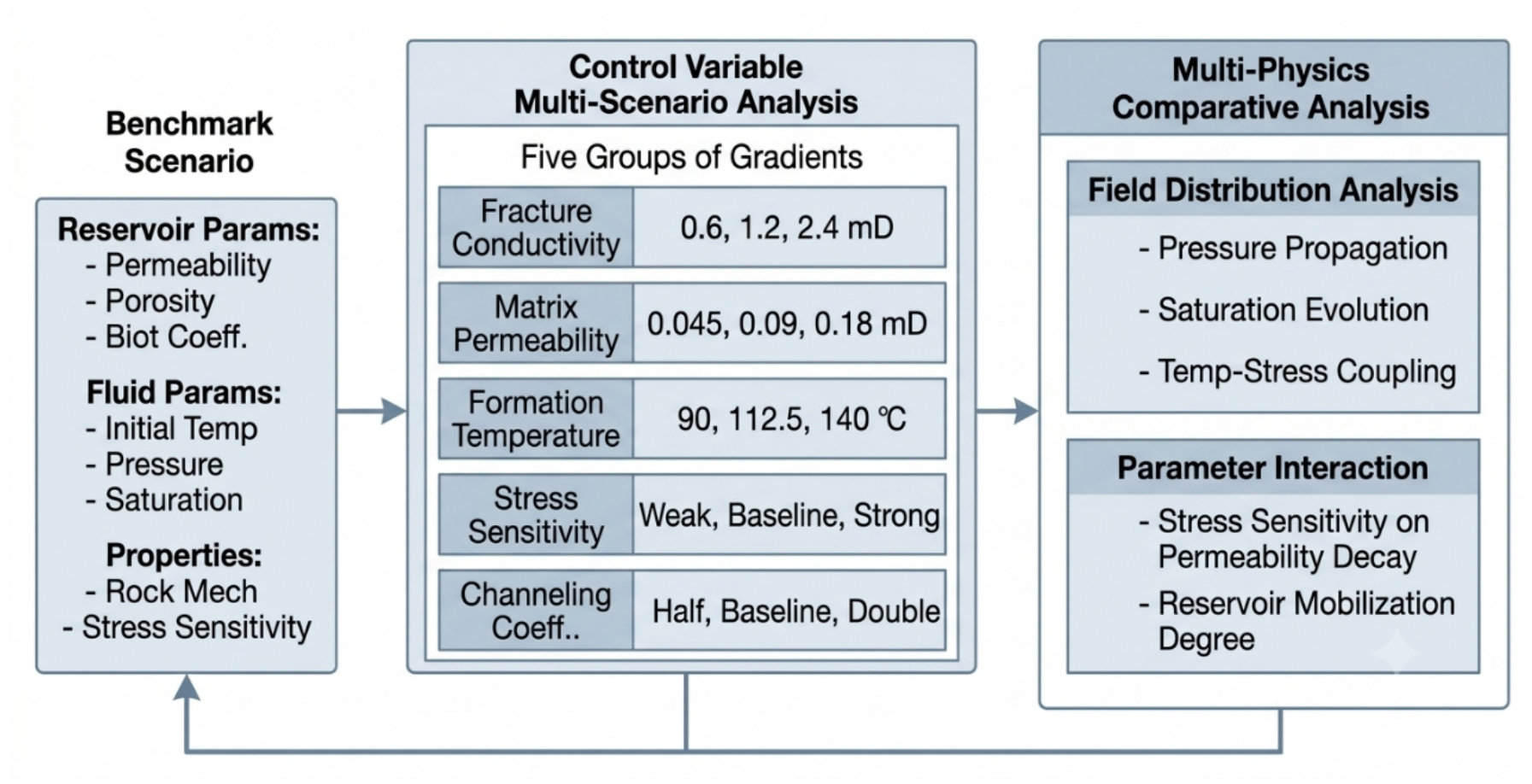
Figure 13.
Illustrative relative ordering of parameter influence. Bar heights visualise the qualitative ranking and are not independently calculated sensitivity indices.
Figure 13.
Illustrative relative ordering of parameter influence. Bar heights visualise the qualitative ranking and are not independently calculated sensitivity indices.
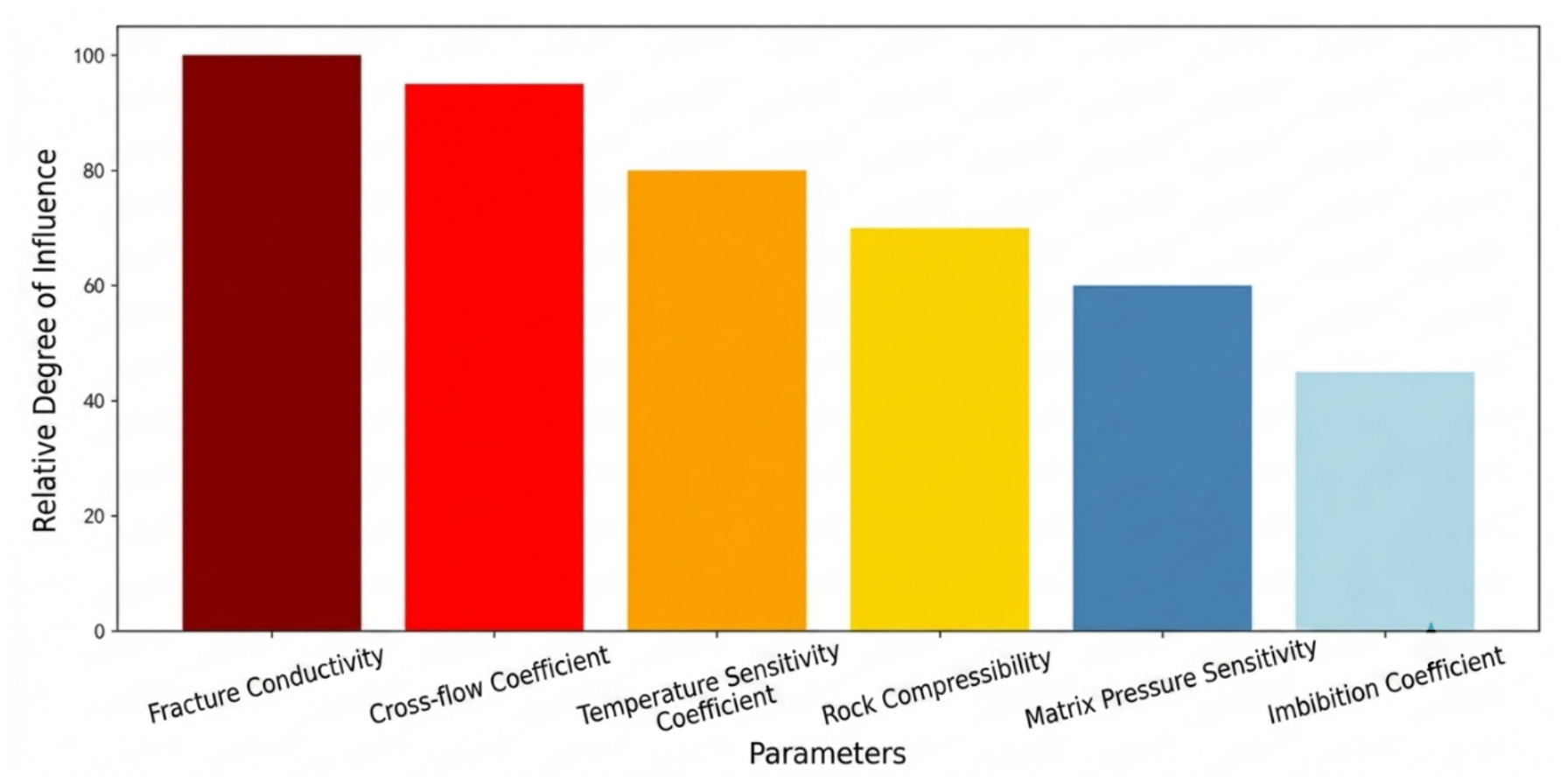
Table 1.
Summary of constitutive and state equations.
| Category | Parameter name | Equation of state |
|---|---|---|
| Fluid properties | Oil-phase density | |
| Water-phase density | ||
| Oil-phase viscosity | ||
| Water-phase viscosity | ||
| Medium properties | Matrix permeability | |
| Fracture permeability | ||
| Fracture conductivity | ||
| Matrix porosity | ||
| Fracture porosity | ||
| Equivalent thermal conductivity | ||
| Coupling & constraints | Fracture–matrix coupling coefficient | |
| Saturation constraint |
Table 2.
Bidirectional coupling mechanisms among thermo-hydro-mechanical fields.
| Coupling direction | Coupling mechanism | Mathematical expression |
|---|---|---|
| Flow field → Stress field | Pore pressure changes effective stress | |
| Stress field → Flow field | Effective stress changes permeability | |
| Temperature field → Flow field | Temperature changes fluid viscosity | |
| Flow field → Temperature field | Fluid flow transports heat by advection | |
| Temperature field → Stress field | Temperature produces thermal strain and thermal stress | |
| Stress field → Temperature field | Rock deformation produces energy dissipation | |
| Dual-medium fluid exchange | Interporosity flow (driven by a pressure difference) | |
| Imbibition (driven by capillary forces) | ||
| Dual-medium property coupling | Fracture → matrix conductivity coupling |
Table 3.
Reported network and training settings.
| Setting | Value or description |
|---|---|
| Input | Three spatial coordinates and time |
| Fourier mapping | Fixed random frequency matrix ; sine and cosine features |
| Hidden layers | 7 layers; 40 neurons per layer |
| Activations | Tanh hidden layers; linear output layer |
| Outputs | , , , , T |
| Optimiser | Adam |
| Initial learning rate | 10-4 |
| Learning rate schedule | Cosine annealing |
| Maximum iterations | 25,000 |
| Stopping criterion | Total-loss change < 10-6 over 2000 consecutive iterations |
| Initial loss weights | |
| Labelled dataset split | Training:test = 9:1 |
| Collocation sampling | Random uniform sampling |
| Loss recording interval | 500 iterations |
Table 4.
Benchmark properties.
| Property | Matrix | Fracture |
|---|---|---|
| Initial permeability (mD) | 0.09 | 1.2 |
| Porosity (dimensionless) | 0.0402 | 0.015 |
| Biot coefficient | 0.92 | 0.98 |
| Initial pressure (MPa) | 82.9 | 82.9 |
| Initial temperature () | 112.5 (shared temperature) | |
| Initial oil saturation | 0.531 | Not specified |
The supplied source places the sole initial oil-saturation value in the matrix column; it does not separately state a fracture value.
Table 5.
Reported values for the baseline PINN and Fourier-PINN.
| Field | Symbol | Baseline PINN | Fourier-PINN |
|---|---|---|---|
| Matrix pressure | 0.410 | 0.923 | |
| Fracture pressure | 0.096 | 0.025 | |
| Matrix oil saturation | 0.415 | 0.923 | |
| Temperature | T | −1.7126 | 0.947 |
Table 6.
One-at-a-time parameter variations.
| Parameter | Reported levels |
|---|---|
| Fracture permeability (mD) | 0.6, 1.2, 2.4 |
| Matrix permeability (mD) | 0.045, 0.09, 0.18 |
| Formation temperature () | 90, 112.5, 140 |
| Stress sensitivity | Weak, benchmark, strong |
| Intercontinuum exchange coefficient | 0.5, 1, and 2 times the benchmark value |
Table 7.
Reported qualitative ordering of parameter influence.
| Rank | Parameter | Reported category |
|---|---|---|
| 1 | Fracture permeability | Extremely high |
| 2 | Intercontinuum exchange coefficient | Extremely high |
| 3 | Temperature sensitivity coefficient | High |
| 4 | Rock compressibility coefficient C | Medium-high |
| 5 | Matrix stress-sensitivity coefficient | Medium |
| 6 | Imbibition coefficient J | Medium-low |
Disclaimer/Publisher’s Note: The statements, opinions and data contained in all publications are solely those of the individual author(s) and contributor(s) and not of MDPI and/or the editor(s). MDPI and/or the editor(s) disclaim responsibility for any injury to people or property resulting from any ideas, methods, instructions or products referred to in the content. |
© 2026 by the authors. Licensee MDPI, Basel, Switzerland. This article is an open access article distributed under the terms and conditions of the Creative Commons Attribution (CC BY) license (http://creativecommons.org/licenses/by/4.0/).
Copyright: This open access article is published under a Creative Commons CC BY 4.0 license, which permit the free download, distribution, and reuse, provided that the author and preprint are cited in any reuse.