

Submitted:
12 October 2026
Posted:
14 October 2026
You are already at the latest version
Abstract
Floating photovoltaic (FPV) systems are an increasingly attractive route to large-scale solar deployment on water bodies, but their structural integrity and energy yield are threatened by the wave environments to which they are exposed at nearshore and offshore sites. Floating breakwaters (FBWs), and keeled geometries in particular, are a candidate protection system. Here we develop a smoothed particle hydrodynamics (SPH) model of a moored, keeled floating breakwater using the open-source solver DualSPHysics, with waves generated by a piston wavemaker with active wave absorption and, for two of the irregular sea states, by the relaxation-zone method (Altomare et al., 2017, 2018). The model is assessed against wave-basin experiments in two stages: a verification stage under regular waves spanning six height–period combinations, and an assessment stage under irregular sea states (two JONSWAP spectra and a broadband white-noise excitation). We report the wave transmission and reflection behaviour, the breakwater motions and their response amplitude operators (RAOs), and find that, once the floating body, the mooring and the incident waves are resolved consistently, the SPH model reproduces the measured heave, roll and sway to within about 20 per cent over most of the regular-wave range and follows the measured RAOs of the irregular sea states, with an accuracy comparable to a boundary-fitted finite-volume model at a fraction of its computational cost.
Keywords:
floating photovoltaics
; floating breakwater
; CFD
; SPH
1. Introduction
As the global demand for renewable energy accelerates, floating photovoltaic (FPV) systems are emerging as a promising response to land scarcity and to the energy–water nexus, allowing solar capacity to be installed on reservoirs, lakes, nearshore and offshore waters [3,4]. Beyond avoiding competition for land, FPV can benefit from the cooling effect of the underlying water body, which raises module efficiency relative to equivalent land-based arrays [5]. The performance of an FPV installation is sensitive to a range of design and environmental parameters, including module layout, float geometry and the local meteo-ocean climate [6].
The transition from sheltered inland waters to open and coastal sites greatly increases the severity of the loading environment. Deployment in open water exposes the array to dynamic wind and wave conditions that threaten both its structural integrity and its energy yield [7,8]. Wave-induced motions drive fatigue at connectors and mooring attachment points, while wind- and motion-induced aerodynamic loads act on the tilted module surfaces [9]. Characterising and mitigating these loads is therefore central to making FPV viable in energetic sites. In practice, commercially deployed FPV systems are largely confined to sheltered inland waters, where the significant wave height rarely exceeds about 0.5 m; marine and near-shore deployments, by contrast, must contend with significant wave heights of the order of 1–2 m and peak periods of several seconds, well beyond the tolerance of most inland designs. Connector and mooring loads scale steeply with wave steepness and height, so even a modest increase in the incident sea state can raise fatigue and ultimate loads at the module interconnections by a large factor [4,7,8], which motivates the use of a dedicated protection structure.
Although FPV platforms can be designed to withstand a range of hydrodynamic conditions, it is often necessary to use floating breakwaters (FBWs) to shield them from the most critical waves that would otherwise endanger their integrity. Compared with fixed, bottom-founded structures, floating breakwaters are attractive because they can be deployed in deeper water, relocated, and tuned to a target sea state by allowing the structure to move and disperse the energy of incoming waves [10]. The design of FBWs frequently incorporates keels or downward-extending skirts, which enhance the structure’s ability to redirect near-surface currents and to further dissipate wave energy. The mechanical performance of an FBW is limited not only by its ability to attenuate waves, but also by the strength of its connection points, which concentrate the largest forces under hydrodynamic loading.
Smoothed particle hydrodynamics (SPH) is a Lagrangian, meshless computational fluid dynamics method well suited to free-surface flows and fluid–structure interaction [11,12]. Because the fluid is discretised into moving particles rather than a fixed grid, SPH naturally handles large free-surface deformation, fragmentation and the moving interfaces produced by floating bodies, situations in which grid-based multiphase approaches such as volume-of-fluid (VOF) can become inaccurate or expensive. SPH has historically been computationally demanding, but the wide availability of graphics processing units (GPUs) has made large simulations tractable. The open-source code DualSPHysics [13] has become a mature platform for GPU-accelerated SPH; it provides a range of SPH formulations together with floating-body dynamics and mooring-line modelling through a coupling to the lumped-mass mooring library MoorDyn(+) [14,15]. SPH has been applied extensively to wave breaking and surf-zone dynamics, building on earlier Eulerian work such as Lin and Liu [16], and increasingly to moored floating structures [15].
In this work we combine wave-basin experiments with numerical simulation to study the dynamics of a moored keeled FBW. We use both SPH (DualSPHysics) and, a finite-volume (FVM) solver (OpenFOAM) to assess the reliability and applicability of these techniques for reducing reliance on costly physical testing. The experiments cover both regular and irregular (JONSWAP and broadband) sea states; the regular cases are used to verify how closely the model can reproduce the measured response, and the irregular cases are then used to assess the model under realistic excitation.
2. Methodology
2.1. Parameter Space and Experiment Layout
The keeled floating breakwater shown in Figure 1 was tested in a wave basin and reproduced in a numerical wave tank. The breakwater is held in place by four soft, taut mooring lines (two per corner pair) whose properties are listed in Table 1; the fairleads attach to the body at and the anchors are fixed at , (model scale). The breakwater geometry and inertial properties, derived by Froude-scaling the full-size design, are summarised in Table 2. All quantities are reported at prototype scale under Froude similitude (length scale ) unless stated otherwise; the conversion factors are given in Section 2.3.1.
The breakwater is oriented broadside to the incoming waves (its long axis parallel to the wave crests). Consequently the wave-frequency response is dominated by sway (horizontal, in the wave-propagation direction), heave and roll; the surge, pitch and yaw responses are comparatively small. This naming convention (sway/heave/roll) is used throughout.
Two families of conditions were tested: a set of regular waves at different wave heights and periods (Section 2.1.1), and a set of irregular waves generated from a JONSWAP spectrum together with a broadband white-noise excitation (Section 2.1.2).
2.1.1. Regular Wave Tests
The regular-wave matrix (Table 3) spans six period–height combinations chosen to cover the operational and design sea states relevant to the protected FPV array. For each case the motions of the breakwater (sway, heave, roll), the surface elevation at wave gauges up- and down-wave of the structure, and the mooring-line tensions were recorded. These provide the reference quantities for verification: the incident wave amplitude, the transmission coefficient and reflection coefficient , and the breakwater motion amplitudes.
2.1.2. Irregular Wave Tests
The irregular matrix (Table 4) comprises two JONSWAP sea states of contrasting steepness and a broadband, near-white excitation that spans the full frequency band of interest. The white-noise case is used to recover the frequency-resolved response (RAOs) and transmission behaviour from a single test. For these cases the reference quantities are the wave spectra, the motion RAOs, and the frequency-dependent transmission coefficient.
2.2. Experimental Methodology Overview
The physical model was tested at a length scale in the wave-basin facility of MARIN (Maritime Research Institute Netherlands) publicly available experimental data was used for comparison. The data can be found in the repository [17]. Wave elevation was measured with an array of resistance-type wave gauges positioned up- and down-wave of the model, the six-degree-of-freedom rigid-body motion was tracked at the body centre of gravity, and the four mooring-line loads were measured at the fairleads.
Because the model was mounted at a 90° heading relative to the solver’s reference frame, the basin-frame channels are mapped to the sway/heave/roll convention used here before comparison. A separate wave-calibration test (without the model present) provides the undisturbed incident spectrum used as the reference for the experimental RAOs, since the gauges nearest the model are locally disturbed by the radiated and diffracted field.
2.3. Numerical Modelling Methodology
2.3.1. Smoothed Particle Hydrodynamics
We model the hydrodynamic forces on the FBW with the weakly compressible SPH solver DualSPHysics (v5.4) [13]. In SPH the fluid domain is discretised into particles whose motion is governed by their mutual interactions. Each particle is advanced by integrating the discrete, weakly compressible form of the mass- and momentum-conservation equations [11,12]:
where and are the velocity and pressure of particle a, and are the mass and density of neighbour b, is gravitational acceleration and is the quintic Wendland kernel [18] with smoothing length in 3D, where is the initial inter-particle spacing. The term is an artificial-viscosity interaction with coefficient . A density-diffusion term following Fourtakas et al. (coefficient ) reduces pressure noise; particle shifting is not used. Closure is provided by the Tait equation of state with polytropic index :
where and is the numerical speed of sound, set to ten times the shallow-water wave speed of the tank, which is still well over an order of magnitude above the wave orbital velocities so that density fluctuations remain below 1%. Time integration uses a Symplectic scheme with a Courant–Friedrichs–Lewy coefficient of . Solid boundaries use the modified dynamic boundary condition (mDBC) with a free-slip condition on the (depth-truncated) floor, which avoids forming a spurious viscous boundary layer on the bed.
All simulations are run at model scale and reported at prototype scale under Froude similitude (; gravity and density invariant). The conversion factors used are: length , time , velocity , acceleration 1, angle 1, frequency , force and mass . The regular-wave cases, JONSWAP 1 and the white-noise case are run with an initial particle spacing of 0.02 m (model scale), which places one particle column inside the 2 cm keels and resolves the 0.20 m draft by ten particle spacings; JONSWAP 2, whose waves are three times higher and longer, is run at 0.04 m to keep its much larger tank affordable. The tank is truncated in depth to about 0.35 times the wavelength (the wave theory used for generation is evaluated at the same depth), and its side walls at 2.3 m from the centreline leave a 0.4 m gap at each end of the breakwater. The resulting models contain between 2.2 and 28.6 million particles. The full parameter set is summarised in Table 5.
Floating Body and Mooring Dynamics
The breakwater is treated as a rigid floating body. The net fluid force and torque are obtained by summing the contributions of the boundary particles that discretise the body, and the rigid-body equations of motion are integrated to update its position and orientation [15]. The hull is filled with boundary particles and the particle lattice is offset so that every wetted face lies half a particle spacing outside the outermost particle layer, the configuration for which the mDBC ghost-node extrapolation is formulated. The four mooring lines are resolved with the lumped-mass model MoorDyn+ coupled to DualSPHysics, which captures line inertia, stiffness, hydrodynamic drag and seabed contact [14,15]; the solver is advanced with its own time step of and an initial dynamic relaxation establishes the static line equilibrium before wave generation. The lines behave as taut linear springs: their unstretched length is set shorter than the fairlead-to-anchor distance so that each line carries a pretension of 9 N and an axial stiffness of 160 N/m (model scale), the values identified from the line tensions of the finite-volume model, which also match the per-line stiffness inferred from the measured load and sway records (about 15.5 kN/m at prototype scale). The pretension keeps the lines taut throughout the regular-wave cases.
Wave Generation and Absorption
The regular waves and JONSWAP 1 are generated by a piston wavemaker placed one wavelength up-wave of the breakwater, driven by second-order (regular) or first-order (irregular) wavemaker theory and equipped with active wave absorption (AWAS), which corrects the paddle motion from the measured free surface so that waves reflected by the breakwater are absorbed at the paddle. A passive damping zone starting 0.75 wavelengths down-wave of the body and extending over one further wavelength dissipates the transmitted waves. The incident wave amplitude was verified against the target for every case with a two-probe decomposition at the body position; where the paddle over- or under-generated by more than 5 per cent (the 3.37, 4.71 and 5.40 s cases), the input wave height was rescaled accordingly and the case re-run, so that the incident wave at the body is within 2 per cent of the target in all regular cases. JONSWAP 2 and the white-noise case are generated with the relaxation-zone (RZ) method developed for SPH by Altomare et al. [1] and refined in Altomare et al. [2], in which a generation zone has its velocity field driven towards the target solution and blended with the SPH field, so that the target waves are imposed while reflected waves travelling back into the band are absorbed [1,2,19]. A start-up ramp is applied in all cases, and the body co-settles with the fluid from the start of the simulation.
2.3.2. Finite Volume Method
As an independent, mesh-based cross-check we reproduced a subset of the regular-wave cases with the open-source finite-volume library OpenFOAM [20]. The two-phase air–water flow is solved with the interFoam solver, which advances the incompressible Navier–Stokes equations for the two immiscible phases and captures the free surface with an algebraic volume-of-fluid (VOF) scheme [21], on a boundary-fitted mesh that conforms to the keeled hull. Regular waves are imposed and absorbed at the domain boundaries, and the breakwater is treated as a rigid six-degree-of-freedom body whose motion is integrated from the resolved pressure and viscous forces on the hull. The four mooring lines are represented with the same lumped-mass model as in the SPH setup, through the MoorDyn coupling [14], so that the geometry, mooring configuration and target waves are identical between the two solvers and the comparison isolates the effect of the discretisation. Only the regular-wave cases were run with the finite-volume model; the irregular sea states were not attempted. The boundary-fitted, fully resolved computations are substantially more expensive per case than the GPU-accelerated SPH simulations, which is the main reason the finite-volume model is used here as a comparison-driven complement rather than as the primary tool. To resolve the motion of the FBW, a mesh morphing technique was used such that the topology around the floating body remained constant and only the positions of the nodes changed, preserving the solid body boundary shape. OpenFOAM v2506 was used and the waves2foam wave generation tool was used at the boundaries to create waves. Simulations were done using a laminar viscous model.
Figure 2.
SPH numerical wave tank with the floating breakwater; colour shows velocity magnitude.
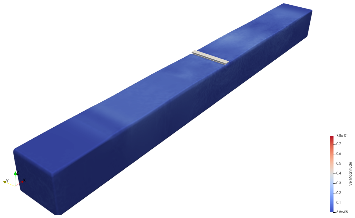
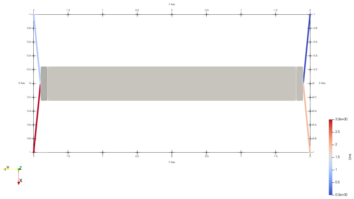
Figure 3.
Plan view of the four-line mooring arrangement; colour indicates line tension. The breakwater long axis is aligned with the crests; waves propagate along x.
Figure 3.
Plan view of the four-line mooring arrangement; colour indicates line tension. The breakwater long axis is aligned with the crests; waves propagate along x.
3. Results
3.1. Regular Wave Analysis
The regular-wave cases verify how closely the SPH model reproduces the measured response condition by condition. Figure 4 shows the wave generation: the incident wave amplitude recovered from a two-probe up-wave decomposition at the body position lies within 2 per cent of the target in every case (panel a). The transmission coefficient rises from 0.31 at 3.37 s to about 0.95 for the longer periods, while the reflection coefficient falls from 0.46 to below 0.05 (panel b).
Figure 5 compares the wave-frequency (first-harmonic) response amplitudes for heave, roll and sway against the experiment. Over the 4.05 to 6.73 s range the SPH model reproduces the measured response closely: sway is within 10 per cent of the experiment, roll is within 4 to 17 per cent and captures the sharp roll peak near 4 s (6.05 deg against 5.77 deg measured), and heave is 5 to 21 per cent below the measurement. At the shortest period, 3.37 s, where the wave height spans only about one particle spacing, all three motions are over-predicted (by 18 to 56 per cent).
3.2. Complementary Finite-Volume Results
As an independent cross-check on the SPH predictions, a subset of the regular-wave cases was reproduced with a boundary-fitted finite-volume (FVM) solver (OpenFOAM). Because the two solvers share the same geometry, mooring configuration and target waves, the comparison isolates the effect of the discretisation approach. The two methods are best viewed as complementary rather than competing, each being most reliable in a different part of the parameter space.
Figure 5 compares the wave-frequency motion amplitudes of experiment, SPH and FVM across the period range. The two numerical models agree with each other and with the measurement to a similar degree. Over the five periods for which FVM motions are available, SPH is closer to the measured sway at four and to the measured roll at four, including the roll peak near 4.05 s (SPH 6.05 deg, FVM 3.87 deg, measured 5.77 deg), while the two models are comparable in heave: SPH is the closer of the two at 4.05, 6.05 and 6.73 s, FVM at 4.71 and 5.40 s. Both models over-predict roll at the longer periods, SPH by 4 to 17 per cent and FVM by 19 to 30 per cent.
Figure 8 shows the phase-aligned time histories at a prototype period of 5.40 s. The three signals are in phase; SPH and FVM both follow the measured sway closely, both are slightly below the measured heave, and SPH follows the measured roll more closely than FVM, which over-predicts it.
Figure 9 compares the wave-frequency amplitude of the fairlead line tension. With the pretensioned spring lines both numerical models follow the measured trend of increasing load with period. SPH is 11 to 22 per cent below the measurement between 4.05 and 6.73 s and above it at 3.37 s, while FVM scatters on both sides of it. The mean pretension of both models (9 N at model scale) is far below that of the physical rig (about 120 to 135 kN at prototype scale); since the lines remain taut in both cases, only the dynamic, wave-frequency amplitude is compared here.
Because the boundary-fitted, fully resolved simulations are considerably more expensive than the GPU-accelerated SPH runs and were applied only to a subset of the regular-wave cases, their role is to bound the discretisation error and to show where the two approaches agree and diverge. The motion comparison is shown in Figure 5 .
3.3. Irregular Wave Analysis
The irregular sea states assess the model under realistic, broadband excitation. The incident spectra measured in the numerical tank reproduce the experimental sea states to different degrees. JONSWAP 2 matches the measured spectrum closely (significant wave height 3.06 m against 3.02 m measured, and within about 10 per cent band by band), whereas JONSWAP 1 reaches 0.71 m against 0.96 m: at the 0.02 m resolution its short waves, a few particle spacings high, lose energy between the wavemaker and the body. The white-noise case carries slightly more energy than measured (0.78 m against 0.64 m) and, because the prescribed velocity series is not spectrally flat, concentrates it between about 1.0 and 1.3 rad/s. Figure 10 shows the response amplitude operators (RAOs) for heave, roll and sway, extracted from the irregular records as the ratio of the response to the incident-wave spectrum, with the three sea states overlapping where their frequency ranges meet. Roll is reported in the non-dimensional form . Because each RAO is normalised by the incident spectrum of its own run, the differences in wave height noted above largely cancel. The SPH RAOs follow the experimental ones in all three degrees of freedom: heave stays close to unity at low frequency and falls off above about 1.8 rad/s as measured, the roll RAO reproduces the measured resonance near 1.4 to 1.6 rad/s in both height and position for the white-noise case and slightly displaced for JONSWAP 1, and sway decays with frequency as in the experiment. The largest departure is the JONSWAP 2 heave RAO above about 1.2 rad/s, where that sea state carries little energy.
Figure 11 shows the frequency-dependent transmission coefficient : the SPH result is compared with the experimental transmission and with the reference curve of Ruol et al [22]. The SPH transmission reproduces the overall roll-off from near-full transmission at low frequency to a minimum of about 0.3 to 0.4 near 1.7 rad/s, but the roll-off occurs about 0.15 to 0.2 rad/s later than in the experiment, and the curves are noisier.
4. Discussion
Taken together, the results indicate that the SPH model reproduces the breakwater motions with an accuracy comparable to that of the boundary-fitted finite-volume model, in both regular and irregular seas, at a fraction of its computational cost. The decisive factors were not the SPH formulation itself but three modelling details. First, the representation of the floating hull: a hull drawn as a single particle shell on its surface loses buoyancy under mDBC and sits several centimetres too deep, which for a body with only 5 cm of freeboard suppresses the heave and, above all, the roll response; filling the hull and offsetting the particle lattice restores the correct draft and the roll resonance. Second, the resolution of the incident waves: with fewer than about two particle spacings across the wave height the short waves lose energy before reaching the body, so their height must be checked and, if needed, corrected at the body position rather than assumed from the wavemaker input.
The remaining discrepancies are modest. Heave is up to about 20 per cent below the measurement at the intermediate periods, roll is slightly over-predicted at the longer periods, and the shortest period, 3.37 s, whose wave height spans only about one particle spacing, is over-predicted in all three motions. In the irregular seas the RAOs are reproduced well, but the JONSWAP 1 waves are generated about a quarter too low at 0.02 m resolution and the white-noise input is not spectrally flat, so the coverage of each frequency band differs from the experiment. The transmission coefficient follows the measured roll-off but is displaced to slightly higher frequencies; since the transmission is the key performance metric for the protected FPV array, a down-wave gauge array that allows a full incident/reflected separation would be a worthwhile addition to future simulations. The breakwater passes most of the long-period energy but strongly attenuates the short, steep waves that are the most damaging to the module interconnections, so it is most effective precisely in the band where the array is most vulnerable.
The mooring and connector loads deserve particular attention because they are the design-limiting quantity for the protected array. The fairlead dynamic tension grows steeply with wave period (Figure 9), and with pretensioned spring lines both numerical models follow this trend, the SPH model 11 to 22 per cent below the measurement between 4.05 and 6.73 s. Because the absolute pretension of the physical rig is far higher than that of the numerical lines, the comparison is restricted to the dynamic load; in the most severe sea state (JONSWAP 2) the numerical lines occasionally go slack, so line loads there should be interpreted with care.
Finally, the behaviour observed here is consistent with the keel playing a central role in dissipating near-surface wave energy. Building on earlier Eulerian free-surface modelling of surf-zone dynamics [16], the present results suggest that the keel redirects and dissipates the incident energy rather than simply reflecting it, and it is this mechanism that allows the structure to attenuate the shorter, steeper waves so effectively.
5. Conclusions
An SPH model of a moored keeled floating breakwater was built in DualSPHysics with piston and relaxation-zone wave generation [1,2] and assessed against wave-basin experiments under both regular and irregular sea states. With a filled, correctly floating hull, pretensioned spring mooring lines and incident waves verified at the body position, the model reproduces the measured sway within 10 per cent and the roll within 4 to 17 per cent over the 4.05 to 6.73 s range, including the sharp roll resonance near 4 s, with heave up to about 20 per cent low. In irregular seas it reproduces the measured heave, roll and sway RAOs, including the roll resonance.
The accuracy of the SPH model is comparable to that of a boundary-fitted finite-volume model (OpenFOAM) run on the regular cases, and better in sway and roll at most periods, while the GPU-accelerated SPH runs are considerably cheaper per case. The SPH model is therefore a practical tool for surveying a broad matrix of sea states, with the finite-volume model useful as an independent cross-check.
The main remaining limitations are the shortest regular period and the high-frequency part of the irregular spectra, where the waves span about one particle spacing, and the transmission coefficient, whose roll-off is displaced to slightly higher frequency than measured. It is also notable that it is more difficult to achieve correct wave generation with the tested wave generation models than with the FVM counterpart.
Acknowledgments
The present study is part of the SUREWAVE project, Funded by the European Union with GA No. 101083342. Views and opinions expressed are however those of the author(s) only and do not necessarily reflect those of the European Union. Neither the European Union nor the granting authority can be held responsible for them.
References
- Altomare, C.; Domínguez, J.M.; Crespo, A.J.C.; González-Cao, J.; Suzuki, T.; Gómez-Gesteira, M.; Troch, P. Long-crested wave generation and absorption for SPH-based DualSPHysics model. Coast. Eng. 2017, 127, 37–54. [Google Scholar] [CrossRef]
- Altomare, C.; Tagliafierro, B.; Domínguez, J.M.; Suzuki, T.; Viccione, G. Improved relaxation zone method in SPH-based model for coastal engineering applications. Appl. Ocean Res. 2018, 81, 15–33. [Google Scholar] [CrossRef]
- Liu, et al. Review of recent offshore floating photovoltaic systems. Energies Rev. 2024. [Google Scholar] [CrossRef]
- Djalab, A.; et al. A comprehensive review of floating photovoltaic systems: technological advances and marine environmental influences. In Renewable and Sustainable Energy Reviews; 2024. [Google Scholar]
- Nysted, et al. Floating photovoltaics: modelled and experimental operating temperatures and the impact of wind speed. Sol. Energy 2024. [Google Scholar] [CrossRef] [PubMed]
- C, J.; et al. Design study on the parameters influencing the performance of floating solar PV. Renew. Energy 2024. [Google Scholar] [CrossRef]
- Mut, et al. Numerical simulation of extreme wave-wind conditions effects on a real field floating photovoltaic plant. Ocean Eng. 2024. [Google Scholar] [CrossRef]
- Zhang, et al. Development of a compliant modular floating photovoltaic farm for coastal conditions. Ocean Eng. 2024. [Google Scholar] [CrossRef]
- Zhang, et al. Aerodynamic effects of an offshore floating photovoltaic platform undergoing pitch and heave motions. Renew. Energy 2024. [Google Scholar] [CrossRef]
- Panjwani, M.K. Assessment of breakwater as a protection system against aerodynamic loads acting on the floating PV. Energies 2024. [Google Scholar] [CrossRef]
- Monaghan, J.J. Smoothed particle hydrodynamics. Annu. Rev. Astron. Astrophys. 1992, 30, 543–574. [Google Scholar] [CrossRef]
- Monaghan, J.J. Simulating free surface flows with SPH. J. Comput. Phys. 1994, 110, 399–406. [Google Scholar] [CrossRef]
- Crespo, A.J.C.; Domínguez, J.M.; Rogers, B.D.; Gómez-Gesteira, M.; Longshaw, S.; Canelas, R.; Vacondio, R.; Barreiro, A.; García-Feal, O. DualSPHysics: Open-source parallel CFD solver based on Smoothed Particle Hydrodynamics (SPH). Comput. Phys. Commun. 2015, 187, 204–216. [Google Scholar] [CrossRef]
- Hall, M.; Goupee, A. Validation of a lumped-mass mooring line model with DeepCwind semisubmersible model test data. Ocean Eng. 2015, 104, 590–603. [Google Scholar] [CrossRef]
- Domínguez, J.M.; Crespo, A.J.C.; Hall, M.; Altomare, C.; Wu, M.; Stratigaki, V.; Troch, P.; Cappietti, L.; Gómez-Gesteira, M. SPH simulation of floating structures with moorings. Coast. Eng. 2019, 153, 103560. [Google Scholar] [CrossRef]
- Lin, P.; Liu, P.L.F. A numerical study of breaking waves in the surf zone. J. Fluid Mech. 1998, 359, 239–264. [Google Scholar] [CrossRef]
- van der Zanden, J. SUREWAVE Basin Test Results. 2025. [Google Scholar] [CrossRef]
- Wendland, H. Piecewise polynomial, positive definite and compactly supported radial functions of minimal degree. Adv. Comput. Math. 1995, 4, 389–396. [Google Scholar] [CrossRef]
- Altomare, C.; et al. DualSPHysics modelling of sea waves: new developments, capabilities and practical examples. In Proceedings of the Proceedings of the SPHERIC Workshop, Tutorial / state-of-the-art review. 2023. [Google Scholar]
- Weller, H.G.; Tabor, G.; Jasak, H.; Fureby, C. A tensorial approach to computational continuum mechanics using object-oriented techniques. Comput. Phys. 1998, 12, 620–631. [Google Scholar] [CrossRef]
- Hirt, C.W.; Nichols, B.D. Volume of fluid (VOF) method for the dynamics of free boundaries. J. Comput. Phys. 1981, 39, 201–225. [Google Scholar] [CrossRef]
- Ruol, P.; Martinelli, L.; Pezzutto, P. Formula to predict transmission for π-type floating breakwaters. J. Waterw. Port. Coast. Ocean Eng. 2013, 139, 1–8. [Google Scholar] [CrossRef]
Figure 1.
Geometry of the keeled floating breakwater (model scale): top, plan view; bottom left, cross-section showing the keel; bottom right, perspective view. Axis units in metres.
Figure 1.
Geometry of the keeled floating breakwater (model scale): top, plan view; bottom left, cross-section showing the keel; bottom right, perspective view. Axis units in metres.
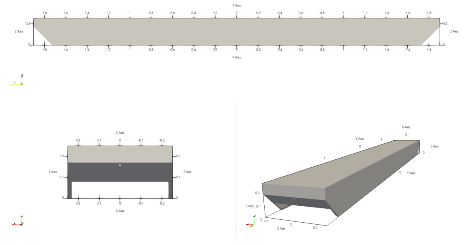
Figure 4.
Regular-wave generation. (a) Incident wave amplitude from a two-probe decomposition of the SPH free surface versus the target; (b) transmission () and reflection () coefficients. Prototype scale.
Figure 4.
Regular-wave generation. (a) Incident wave amplitude from a two-probe decomposition of the SPH free surface versus the target; (b) transmission () and reflection () coefficients. Prototype scale.
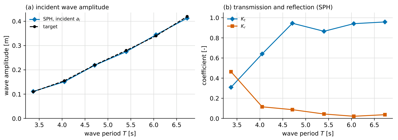
Figure 5.
Regular-wave motion response: wave-frequency amplitude of heave, roll and sway from experiment, SPH and FVM (OpenFOAM). FVM motion data are available at five periods (4.05, 4.71, 5.40, 6.05 and 6.73 s). Prototype scale.
Figure 5.
Regular-wave motion response: wave-frequency amplitude of heave, roll and sway from experiment, SPH and FVM (OpenFOAM). FVM motion data are available at five periods (4.05, 4.71, 5.40, 6.05 and 6.73 s). Prototype scale.
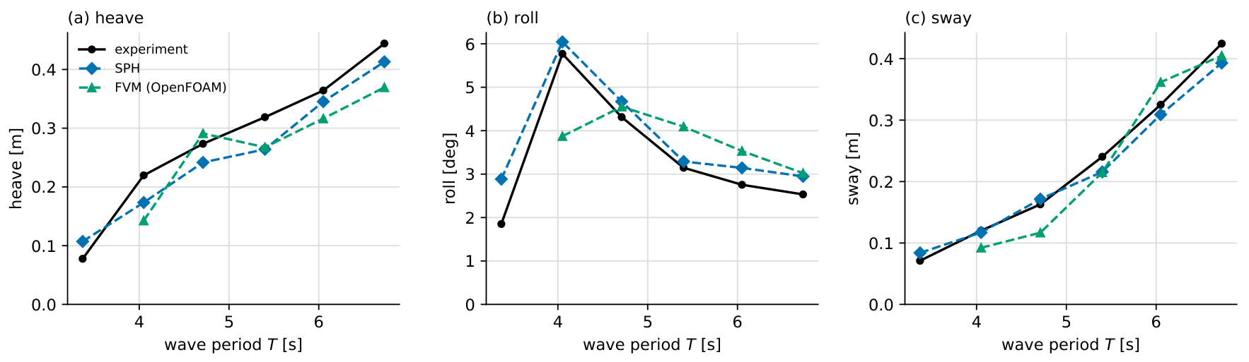
Figure 6.
Regular-wave time-domain agreement at four of the six periods: phase-aligned heave, roll and sway, SPH versus experiment. Prototype scale.
Figure 6.
Regular-wave time-domain agreement at four of the six periods: phase-aligned heave, roll and sway, SPH versus experiment. Prototype scale.
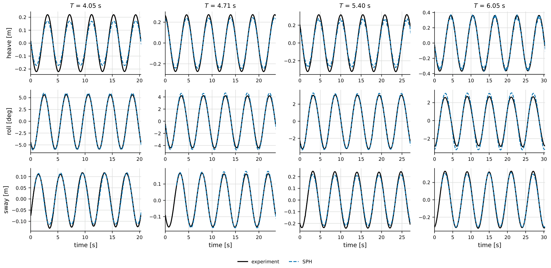
Figure 7.
Supplementary: regular-wave time-domain agreement for all six periods, SPH versus experiment. Prototype scale.
Figure 7.
Supplementary: regular-wave time-domain agreement for all six periods, SPH versus experiment. Prototype scale.
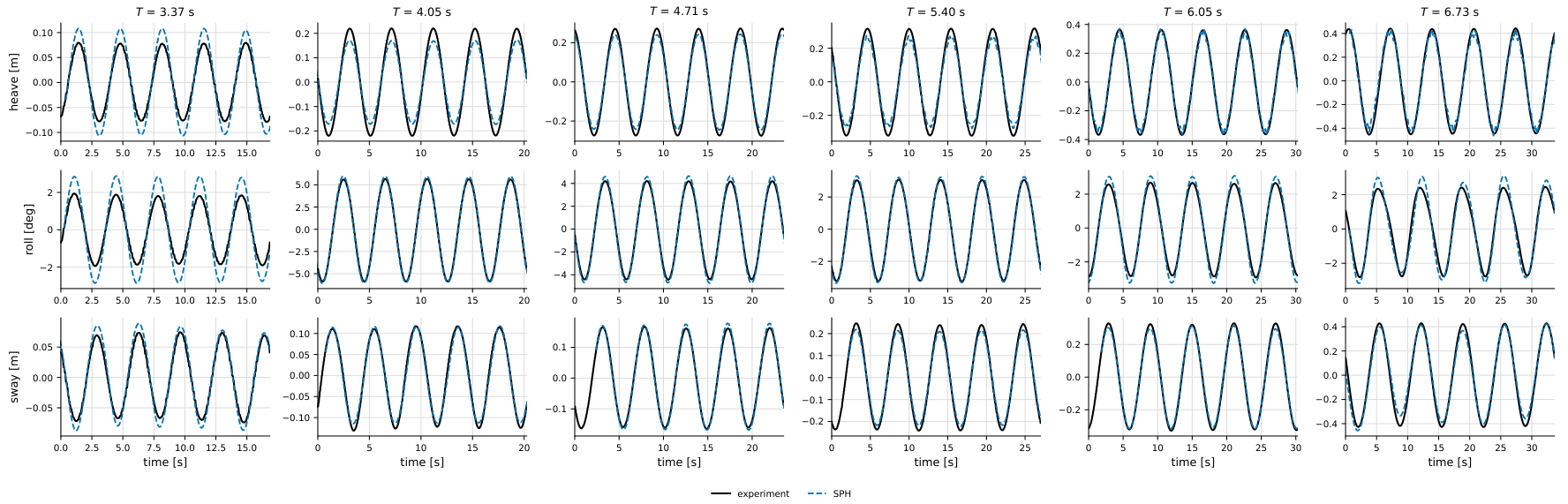
Figure 8.
Regular-wave time-domain agreement at a period of 5.40 s: phase-aligned heave, roll and sway from experiment, SPH and FVM (OpenFOAM). Prototype scale.
Figure 8.
Regular-wave time-domain agreement at a period of 5.40 s: phase-aligned heave, roll and sway from experiment, SPH and FVM (OpenFOAM). Prototype scale.
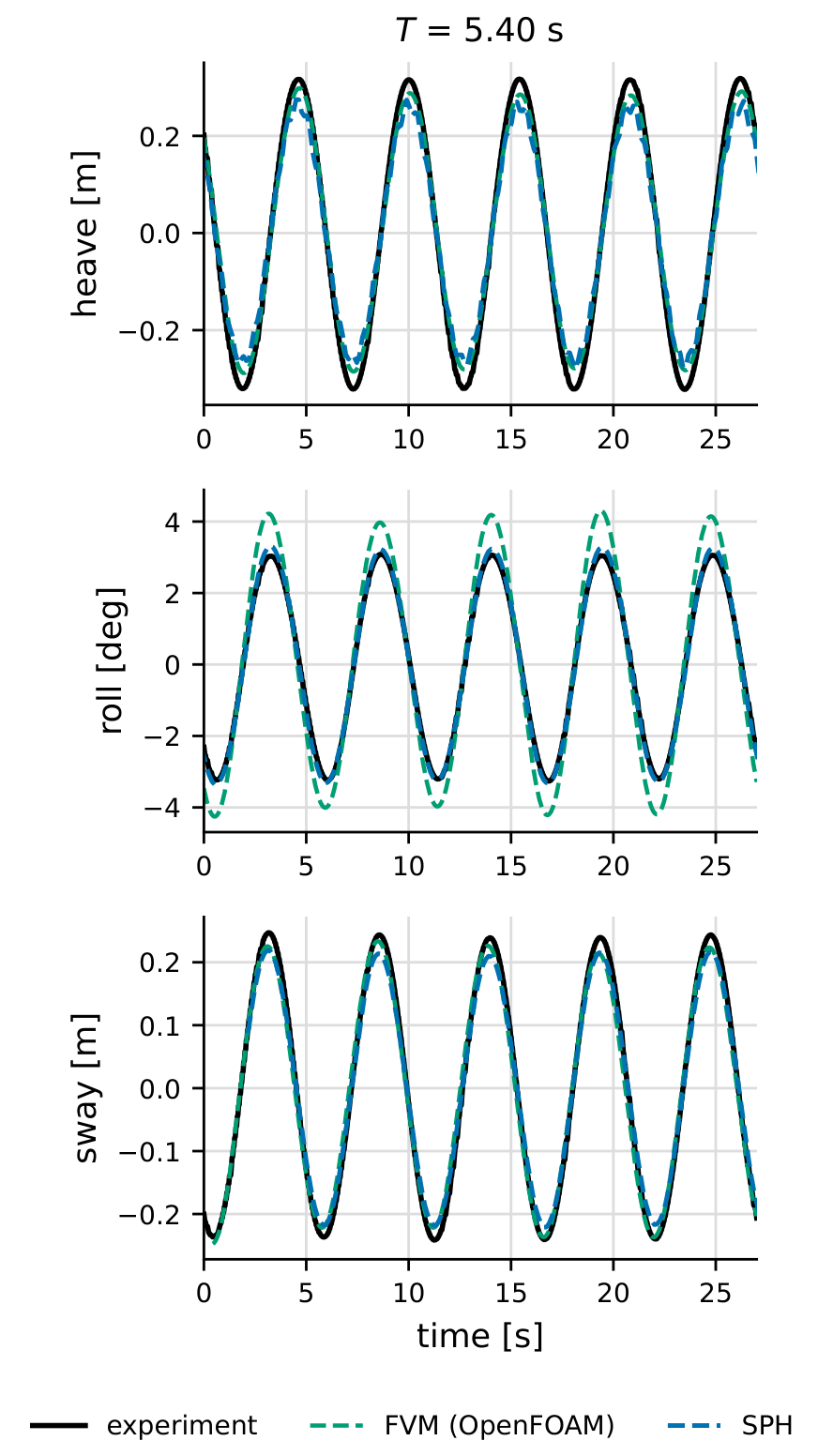
Figure 9.
Fairlead mooring-line load: wave-frequency (dynamic) tension amplitude of the most heavily loaded line versus wave period, from experiment, SPH and FVM (OpenFOAM). Only the dynamic amplitude is compared, as the pretension of the numerical lines differs from that of the physical rig. Prototype scale.
Figure 9.
Fairlead mooring-line load: wave-frequency (dynamic) tension amplitude of the most heavily loaded line versus wave period, from experiment, SPH and FVM (OpenFOAM). Only the dynamic amplitude is compared, as the pretension of the numerical lines differs from that of the physical rig. Prototype scale.
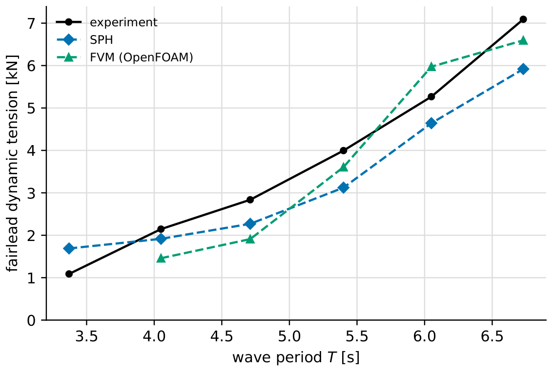
Figure 10.
Response amplitude operators from the irregular sea states: heave, roll [] and sway, SPH (solid) versus experiment (dashed). Prototype scale.
Figure 10.
Response amplitude operators from the irregular sea states: heave, roll [] and sway, SPH (solid) versus experiment (dashed). Prototype scale.
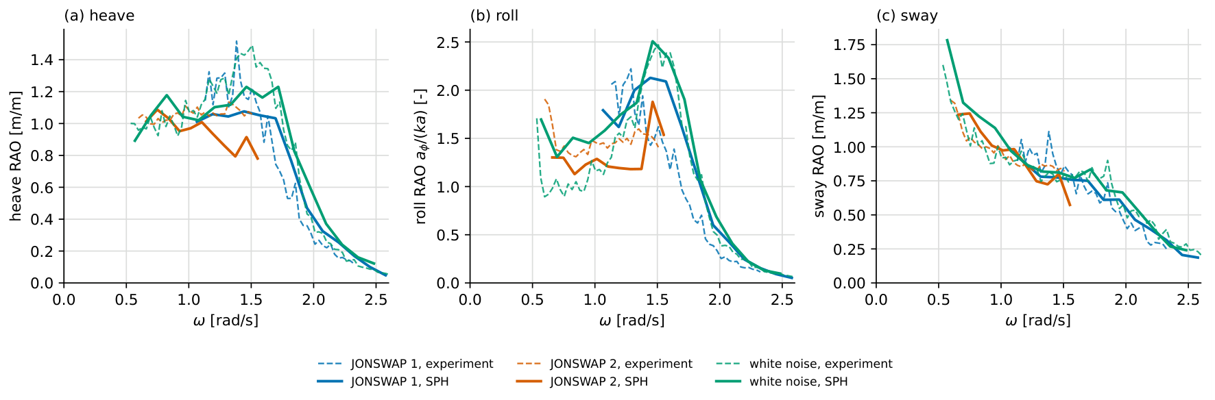
Figure 11.
Frequency-dependent transmission coefficient for the irregular sea states: SPH versus experiment and a literature reference. The experimental and reference curves are approximate (digitized). Prototype scale.
Figure 11.
Frequency-dependent transmission coefficient for the irregular sea states: SPH versus experiment and a literature reference. The experimental and reference curves are approximate (digitized). Prototype scale.
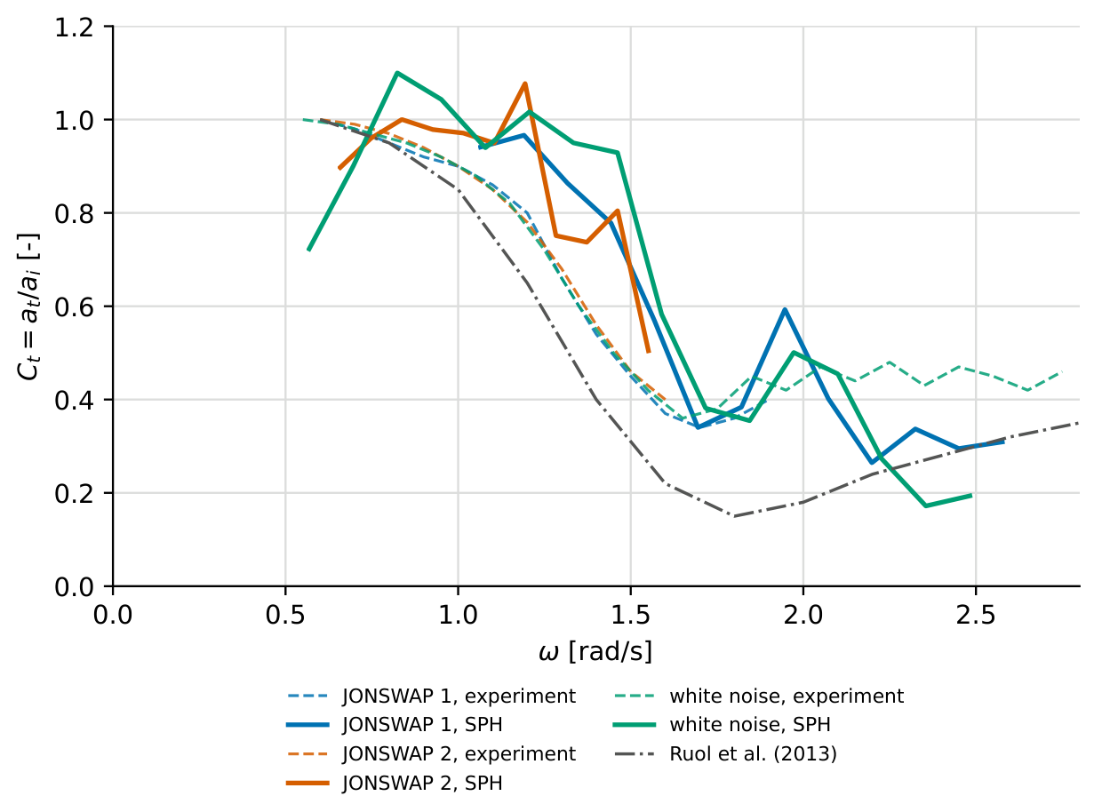

Table 1.
Mooring-line properties (MoorDyn+ lumped-mass model), as run at model scale. All four lines share the same properties. Fairlead-to-anchor distance 1.005 m; the shorter unstretched length gives the pretension.
Table 1.
Mooring-line properties (MoorDyn+ lumped-mass model), as run at model scale. All four lines share the same properties. Fairlead-to-anchor distance 1.005 m; the shorter unstretched length gives the pretension.
| Property | Symbol | Value (model) |
|---|---|---|
| Unstretched length | 0.949 m | |
| Axial stiffness | 152 N | |
| Line stiffness | 160 N/m | |
| Pretension | 9 N | |
| Equivalent diameter | D | 0.01 m |
| Mass per unit length (air) | w | 0.08 kg/m |
| Internal damping () | – | |
| Transverse drag coeff. | 1.2 | |
| Tangential drag coeff. | 0.05 | |
| Transverse added mass | 1.0 | |
| Segments per line | – | 10 |
| Number of lines | n | 4 |
Table 2.
Floating breakwater inertial properties (model scale).
| Property | Symbol | Value |
|---|---|---|
| Mass | m | 238 |
| Centre of gravity (above keel) | – | |
| Width | B | meter |
| Length | L | |
| Keel depth | ||
| Inertia () | – | |
| Inertia () | – | |
| Inertia () | – |
Table 3.
Regular-wave test matrix (prototype scale). T is the wave period, H the wave height.
| Case | T () | H () |
|---|---|---|
| R1 | 3.37 | 0.22 |
| R2 | 4.05 | 0.31 |
| R3 | 4.71 | 0.44 |
| R4 | 5.40 | 0.56 |
| R5 | 6.05 | 0.68 |
| R6 | 6.73 | 0.84 |
Table 4.
Irregular-wave test matrix (prototype scale). is the peak period, the significant wave height and the JONSWAP peak-enhancement factor. The white-noise case is a broadband excitation covering the period band .
Table 4.
Irregular-wave test matrix (prototype scale). is the peak period, the significant wave height and the JONSWAP peak-enhancement factor. The white-noise case is a broadband excitation covering the period band .
| Case | Spectrum | () | () | |
|---|---|---|---|---|
| J1 | JONSWAP | 4.0 | 1.0 | 4.00 |
| J2 | JONSWAP | 7.5 | 3.1 | 2.34 |
| W | white noise | – | 0.67 | – |
Table 5.
Numerical parameters of the SPH model.
| Parameter | Value |
|---|---|
| Solver | DualSPHysics v5.4 (GPU) |
| Initial particle spacing | 0.02 m (JONSWAP 2: 0.04 m) |
| Smoothing-length coefficient | |
| Kernel | Wendland (quintic) |
| Viscosity treatment | Artificial, |
| Density diffusion | Fourtakas, |
| Particle shifting | disabled |
| Reference density | 1000 |
| Speed-of-sound coefficient | 10 |
| Time integration | Symplectic |
| CFL number | 0.2 |
| Boundary condition | mDBC, free-slip floor |
| Floating body | filled hull, lattice offset dp/2 |
| Rigid-body algorithm | SPH |
| Wave generation | piston + AWAS; RZ (JONSWAP 2, white noise) |
| Tank depth | about 0.35 wavelengths |
| Mooring model | MoorDyn+, |
| Froude length scale | 10 |
| Number of particles | 2.2 to 28.6 million |
Disclaimer/Publisher’s Note: The statements, opinions and data contained in all publications are solely those of the individual author(s) and contributor(s) and not of MDPI and/or the editor(s). MDPI and/or the editor(s) disclaim responsibility for any injury to people or property resulting from any ideas, methods, instructions or products referred to in the content. |
© 2026 by the authors. Licensee MDPI, Basel, Switzerland. This article is an open access article distributed under the terms and conditions of the Creative Commons Attribution (CC BY) license (http://creativecommons.org/licenses/by/4.0/).
Copyright: This open access article is published under a Creative Commons CC BY 4.0 license, which permit the free download, distribution, and reuse, provided that the author and preprint are cited in any reuse.