

Submitted:
28 September 2026
Posted:
29 September 2026
You are already at the latest version
Abstract
Proton exchange membrane (PEM) water electrolysis is a key technology for converting renewable electricity into green hydrogen, and the availability of electrolyser stacks directly determines the hydrogen output and economics of such plants. This paper extends a previously reported ten-state semi-Markov reliability model of a PEM electrolyser into a twenty-state framework that better reflects field behavior. The extension adds a derated, partial-output operating state for each of four degradation mechanisms (membrane, electrode, chemical and thermal), a spares-waiting state that separates logistics delay from active repair, a scheduled preventive-maintenance branch, and a rare catastrophic-shock branch, all treated as competing risks at the operative state. Closed-form steady-state expressions are derived for availability, mean time to system failure (MTSF) and maintenance-crew busy periods. A delta-method procedure converts sensitivity coefficients into a confidence interval on availability, and a profit function balances hydrogen revenue against inspection, derating, logistics and repair costs. Using plant rates from a pilot-scale electrolyser and literature-informed values for the new parameters, the model gives a steady-state availability of 0.8804 (95% CI: 0.778–0.983), an MTSF of about 5270 h and an illustrative profit rate of $383.28/h. The results show that models omitting preventive maintenance and shock-type failures overstate electrolyser availability, with direct consequences for hydrogen supply planning and plant economics.
Keywords:
PEM electrolyser
; green hydrogen
; water electrolysis
; semi-Markov process
; multi-state reliability
; derated operation
; logistics delay
; availability
; cost–benefit analysis
I. Introduction
Green hydrogen produced by water electrolysis using renewable electricity is widely regarded as a key energy carrier for decarbonizing industry, heavy transport and long-duration energy storage [1,2]. Among electrolysis technologies, PEM electrolysers are favored for coupling with variable solar and wind power because of their fast dynamic response, compact design and high current density [2,3]. However, their stacks degrade through membrane thinning, catalyst loss, chemical contamination and thermal stress, and this degradation raises specific energy consumption and ultimately forces the unit out of service [4,5,6,7]. Every hour of downtime or reduced-capacity operation is an hour of lost hydrogen production and unused renewable electricity. The availability of an electrolyser is therefore not only a maintenance concern but a determinant of the cost and security of hydrogen supply. This is especially relevant in countries such as Oman, which has made green hydrogen a pillar of its energy transition strategy [8]. Reliable, data-driven models of electrolyser availability are needed to plan maintenance, size spare-part inventories and estimate the true production capacity of hydrogen plants.
Reliability modelling of hydrogen-generation systems has matured considerably over the last two decades, with Markov and semi-Markov processes remaining the dominant probabilistic tools for capturing transitions across operational states [9,10,11]. A recurring limitation in this body of work, however, is that component and subsystem degradation is almost always represented as a binary transition — a unit is either functioning or has failed — even though many electro-mechanical and electrochemical systems degrade gradually and continue to deliver reduced, rather than zero, output for extended periods [12,13]. Such models have recently begun to be applied to green-hydrogen plants, for example to the power-supply chain of electrolysers through a Bayesian continuous-time Markov chain [14], while a review of incidents in water-electrolysis plants found that reliability engineering is still little applied in the hydrogen sector despite the cost of unplanned downtime [15]. Reliability models of the electrolyser stack itself, which is where the degradation mechanisms act, remain scarce.
Reliability, availability and maintainability (RAM) studies across a wide range of industrial plants — desalination units [16,17,18], soft-water treatment [19], wastewater treatment [20], concrete and sugar processing [21,22], cable manufacturing and aluminium production [23,24,25,26,27,28], steam-turbine generators [29], power transformers [30,31], and power distribution networks [32] — have consistently demonstrated the practical value of structured multi-state reliability analysis for maintenance planning. Best-fit distribution selection for repair and restoration data has likewise been shown to materially improve the accuracy of reliability indices in complex installations [33,34]. A prior study by the present authors introduced a ten-state semi-Markov framework for PEM electrolyser that classified anomalies into membrane, electrode, chemical and thermal degradation states before transitioning to corresponding failed states, and benchmarked the probabilistic availability against ARIMA and Random Forest forecasts [35].
That earlier framework, while establishing the basic state architecture for electrolyser degradation, shares the binary-outcome limitation of the wider literature: it does not distinguish a partially degraded but still-producing system from a fully failed one, it does not separate the time a maintenance crew spends waiting for spare parts from the time actually spent repairing — a distinction long recognized in maintainability engineering as administrative and logistics delay time (ALDT) versus active corrective-maintenance time [36] — and it does not admit a sudden, non-degradation-path failure such as a common-cause electrical or pressure shock. The broader multi-state-systems literature has meanwhile developed the formal machinery for exactly this kind of graceful-degradation modelling [12,13,37], and has shown that rare shock-type failures competing with gradual degradation paths can be incorporated into a single stochastic framework without sacrificing tractability [13].
The present paper closes these gaps for the PEM electrolyser case. It extends the ten-state model of [35] into a twenty-state semi-Markov framework that (a) inserts a derated, partial-capacity operating state between each degradation state and its corresponding failed state; (b) inserts a spares-waiting state ahead of each active-repair state, so that logistics delay is estimated separately from repair duration; (c) introduces a scheduled preventive-maintenance branch competing with the anomaly-detection path at the operative state; and (d) introduces a rare catastrophic common-cause shock branch, also competing at the operative state. Beyond the state-space extension, this paper makes three further contributions absent from [35]: a delta-method procedure that converts rate-sensitivity coefficients into a defensible 95% confidence interval on steady-state availability; closed-form mean-time-to-system-failure (MTSF) expressions obtained through a regenerative argument; and a steady-state profit (cost-benefit) function that nets hydrogen-revenue accrual against inspection, derating, logistics and repair costs, in the spirit of profit-function formulations used elsewhere in the RAM literature [19,22,38].
The remainder of the paper is organized as follows. Section II summarizes the available plant data and the literature-informed assumed values used to instantiate the newly introduced states. Section III defines the extended state space and presents the transition diagram. Section IV derives the governing transition-probability, availability, MTSF and busy-period equations, each accompanied by its steady-state numerical evaluation. Section V develops the confidence-interval procedure. Section VI formulates the profit function. Section VII reports consolidated numerical results and discussion, and Section VIII concludes.
II. Data Summary
Table 1 reports the plant rates previously reported in [35], available from three years of pilot-scale PEM electrolyser maintenance records. Table 2 reports the assumed values used to instantiate the newly introduced states; because no field data yet exist for these parameters at the case-study plant, values are set within ranges reported for scheduled-maintenance cadence, shock-type competing-failure rates in multi-state systems [13], and spares logistics delay per maintainability guidance [36]. All numerical results in this paper (Sections IV–VII) are computed from Table 1 and Table 2 and should be read as illustrative of the framework rather than as validated plant-specific forecasts.
III. System Description and Extended State Space
A. Overview
Continuous monitoring of cell voltage, current, hydrogen production rate and temperature is assumed, as in [35]. Unlike the original model, the operative state S0 now competes among three mutually exclusive, exponentially distributed sojourn-terminating events: anomaly detection (rate α), the onset of a scheduled preventive-maintenance interval (rate δ), and a rare catastrophic shock (rate θ). Once an anomaly is confirmed, diagnostics classify it into one of four degradation states (S2–S5) exactly as in [35]. Each degradation state now feeds a derated operating state (S6–S9) representing continued, reduced-capacity hydrogen production — rather than an immediate jump to full failure — which subsequently feeds a spares-waiting state (S10–S13) and finally an active-repair state (S14–S17). All repair, preventive-maintenance and catastrophic-overhaul completions return the system to S0. The twenty states are summarised in Table 3. This graceful-degradation structure is consistent with experimental evidence that PEM stacks lose performance progressively rather than abruptly, at rates that depend on the operating mode and increase under intermittent operation [39,40].
B. Transition Diagram
Figure 1 gives a block schematic of the twenty states grouped by category and degradation mechanism, and Figure 2 shows the corresponding state-transition diagram with every rate marked on its edge; the meaning of each rate symbol is summarised in the legend of Figure 2 and in Table I. Solid arrows denote the anomaly-driven diagnostic path and its four mechanism-specific degradation→derated→waiting→repair chains; dashed arrows denote the rare catastrophic-shock branch. All repair states (S14–S17) and the catastrophic state S18 return the system directly to S0, as does the preventive-maintenance state S19.
C. Modelling Assumptions
(1) The system starts in S0. (2) Sojourn times at S0 for the three competing exit events are independent exponential random variables; the transition actually observed is the one with the shortest realised time (a standard competing-risks construction). (3) Diagnostic classification (S1 → S2–S5) follows the same probabilities pm, pe, pc, pt as in [35], with pm+pe+pc+pt = 1. (4) Within each degradation branch the progression degradation → derated → waiting → repair → operative is deterministic (transition probability 1 at each step), consistent with the physical picture that an unaddressed degradation mechanism worsens monotonically until repaired. (5) Preventive maintenance and catastrophic overhaul each return the system directly to S0. (6) Failure and shock inter-arrival times are exponential; repair, waiting and derated-operation sojourns may in general follow arbitrary distributions, which is why the process remains a semi-Markov process even though the numerical illustration in this paper uses exponential rates throughout for tractability, exactly as justified in [35].
IV. Mathematical Formulation
A. Notation Recap
Si, Sj denote states (i, j = 0 to 17, plus 18, 19); qij(t) and Qij(t) are as defined in the Notation section. © denotes the Laplace convolution operator. Ai(t) is the probability that the electrolyser is in an up (producing) state at time t given it was in Si at t = 0. Bi(t) is the probability that the maintenance crew is occupied (inspection, waiting, or active repair) at time t given the system was in Si at t = 0.
B. Transition Probability Densities
The competing-risks structure at S0 gives three simultaneous transition densities:
with branching probabilities obtained by integrating (1a)–(1c) over t and normalising by the total exit rate (α+δ+θ):
dQ01(t) = α e−αt dt
dQ0,19(t) = δ e−δt dt
dQ0,18(t) = θ e−θt dt
Diagnostic classification from S1 follows the same form as [35], with destination j = 2, 3, 4, 5 and corresponding probability pj ∈ {pm, pe, pc, pt}:
dQ1j(t) = pj β e−βtdt
For each degradation mechanism k = 1 (membrane), 2 (electrode), 3 (chemical), 4 (thermal), the deterministic progression through derating, spares-waiting and active repair is governed by:
where deg(k), der(k), wait(k), rep(k) denote the four mechanism-specific states in sequence (e.g., for k = 1 / membrane: S2 → S6 → S10 → S14), and λk, λ′k, νk, γk are the degradation-to-derated, derated-to-waiting, waiting-to-repair and repair-to-operative rates respectively. The preventive-maintenance and catastrophic branches close as:
dQ19,0(t) = ε e−εt dt, dQ18,0(t) = φ e−φt dt
C. Mean Sojourn Times
Using μi = E[sojourn time in Si], the sojourn times follow directly from (1)–(5):
μdeg(k) = 1/λk, μder(k) = 1/λ'k, μwait(k) = 1/νk, μrep(k) = 1/γk (k = 1,…,4)
D. Steady-State Availability
Following the regenerative-process argument used for the base model [35], the probabilities Ai(t) satisfy a system of Markov-renewal integral equations whose Laplace transforms yield, after inversion at s → 0, the steady-state availability
where the numerator equals the mean sojourn time at S0,
and the denominator sums, over one regeneration cycle, the mean time spent in every state weighted by the probability of actually visiting that state starting from S0:
with each branch term Bk (k = m, e, c, t) the sum of the four mechanism-specific sojourn times encountered from disturbance to repair completion:
N1 = μ0
D1 = μ0 + p01[ μ1 + pm · Bm + pe · Be + pc · Bc + pt · Bt ] + p0,19μ19 + p0,18μ18
Bk = μdeg(k) + μder(k) + μwait(k) + μrep(k)
Substituting the plant rates of Table 1 and the assumed rates of Table 2 into (6)–(10) gives μ0 = 629.37 h, D1 = 714.84 h, and hence the steady-state numerical outcome
Equations (7)–(10) reduce exactly to Equation (12) of [35] when δ = θ = 0 and μder(k) = μwait(k) = 0 for all k, confirming that the original ten-state model is the special case of the present framework in which no preventive maintenance, no catastrophic shocks, and no derated or logistics-delay states are recognized.
E. Mean Time to System Failure
Treating the four active-repair states and the catastrophic state as momentarily absorbing (i.e., computing the expected time to first reach a state requiring active intervention), a regenerative argument analogous to (7)–(10) gives, for each mechanism k, the expected time to reach the corresponding repair state,
which combine at S1 as
and, accounting for the fact that a preventive-maintenance excursion is a renewal that does not itself count toward failure,
where T0 is the mean time to system failure (MTSF). Substituting the parameter values of Table 1 and Table 2 gives T1 = 5,915.4 h and, since p0,19 = 0.8741 and p01 = 0.0944, the steady-state numerical outcome
Tk = μdeg(k) + μder(k) + μwait(k) (k = m, e, c, t)
T1 = μ1 + pm · Tm + pe · Te + pc · Tc + pt · Tt
F. Maintenance-Crew Busy Periods
By the same regenerative argument, the steady-state fraction of time the maintenance crew spends in any state Sj is the product of the probability of reaching Sj from S0 in one cycle and the mean sojourn time at Sj, normalised by D1:
Bj = (path − probability to Sj) × μj / D1
Applied to the preventive-maintenance and catastrophic branches, (14) gives
and, for the membrane branch (k = m) taken as a worked example, (14) decomposes into four separately identifiable busy-period contributions:
Bpm = p0,19μ19 / D1 = 0.004891, Bcat = p0,18μ18 / D1 = 0.010565
Bdeg(m) = 0.019810, Bder(m) = 0.003962, Bwait(m) = 0.001902, Brep(m) = 0.016508
Equation (14) recovers the busy-period expressions of [35] (their Equation (13)) when applied to S1 through S4, and additionally yields separate busy-period contributions for derated operation, spares-waiting and active repair for every mechanism — the maintainability distinction absent from the base model. The full set of busy-period fractions for all four mechanisms is reported in Table 5 (Section VII).
V. Confidence-Interval Estimation
Reliability rates estimated from a finite maintenance record (r̂ = n/T, with n observed events over exposure time T) carry sampling uncertainty that a point estimate of A0 conceals. Rather than introduce a separate variance model, this paper reuses the partial-derivative (sensitivity) coefficients already computed for RAM sensitivity analysis — e.g., ∂A0/∂α, ∂A0/∂λk — as the ingredients of a first-order (delta-method) variance propagation.
For an exponential-rate MLE r̂ = n/T, the asymptotic variance is
Var(r̂) ≈ r̂2 / n
Treating the rate parameters as approximately independent, the delta method gives
and the corresponding 95% confidence interval for steady-state availability is
Evaluating (15)–(17) numerically (Table 6, Section VII) with illustrative observed-event counts consistent with a 3-year maintenance record gives Var(A0) = 2.748×10⁻³, so that the steady-state numerical outcome is
i.e., a 95% confidence interval of A0 ∈ [0.778, 0.983]. The partial derivatives in (16) are obtained here by numerical (finite-difference) perturbation of (7)–(10) about the baseline rates, which reduces to the analytical sensitivity coefficients of [35] in the limiting case of the original ten-state model. Where the exponential-MLE assumption in (15) is judged too strong — for instance where repair-time data are visibly non-exponential — a non-parametric bootstrap over the maintenance log (resampling repair/failure records with replacement and recomputing A0 many times) is recommended as a robustness check; it requires no distributional assumption but is not pursued numerically in this paper.
VI. Cost-Benefit (Profit) Model
Following the profit-function convention used elsewhere in the RAM literature [19,22,38], a steady-state profit rate is defined by netting the revenue accrued while the plant is fully operative against the cost rate of every non-productive activity:
where K0 is the revenue rate accrued per unit time of full-capacity hydrogen production; Kpm and Kcat are the cost rates of preventive maintenance and catastrophic overhaul respectively; and for each mechanism k, Kd,k, Kw,k and Kr,k are, respectively, the revenue-loss-equivalent cost of derated operation, the spares-logistics holding cost, and the active-repair cost rate. Because the derated states now carry their own (reduced) revenue term implicitly through Kd,k rather than being counted as full downtime, Equation (18) is a genuine improvement over a two-state up/down costing model. Because the revenue rate can be written as K0 = ṁH2·cH2, where ṁH2 is the rated hydrogen output of the stack (kg/h) and cH2 is the hydrogen sale price ($/kg), the illustrative value K0 = $500/h corresponds, for example, to a stack producing 100 kg/h of hydrogen sold at $5/kg; plant-specific values of ṁH2 and cH2 can be substituted directly. Substituting the illustrative cost rates of Table 7 (Section VII) into (18) gives the steady-state numerical outcome
P = 440.22 − 0.20 − 15.85 − 14.43 − 14.07 − 7.66 − 4.73 ≈ $383.28 / h
VII. Numerical Results and Discussion
Sections IV–VI derived the governing equations and evaluated each symbolically alongside its steady-state numerical outcome, using the plant rates of Table 1 and the assumed rates of Table 2. This section consolidates those outcomes and discusses their implications.
A. Availability, MTSF and Busy Periods
Table 4 summarises the steady-state indices obtained from (7)–(14). The availability of 0.8804 is lower than the 0.9115 reported for the ten-state model in [35]; the reduction is attributable entirely to the two branches absent from the earlier model — scheduled preventive maintenance and catastrophic overhaul — which together account for roughly 1.5% of system time even though each individual event is either brief (PM) or rare (catastrophic shock). This illustrates the paper’s central methodological point: a purely corrective-maintenance, binary-state model systematically overstates availability by omitting classes of downtime that do not arise from gradual degradation.

Table 4.
STEADY-STATE RESULTS.
| Index | Value |
| A0 (steady-state availability) | 0.8804 |
| 95% CI for A0 (delta method) | [0.7777, 0.9832] |
| MTSF | 5269.6 h ≈ 219.6 days ≈ 0.60 yr |
| Bpm (PM busy fraction) | 0.004891 |
| Bcat (catastrophic busy fraction) | 0.010565 |
| B1 (diagnostic busy fraction) | 0.000088 |
Table 5.
BUSY-PERIOD FRACTIONS BY DEGRADATION MECHANISM (SUM OF ALL 20-STATE FRACTIONS = 1.000).
| Mechanism | Degradation | Derated | Waiting (logistics) | Active repair |
| Membrane | 0.019810 | 0.003962 | 0.001902 | 0.016508 |
| Electrode | 0.001321 | 0.001057 | 0.001268 | 0.022968 |
| Chemical | 0.001057 | 0.000880 | 0.000951 | 0.010565 |
| Thermal | 0.013206 | 0.001651 | 0.000317 | 0.006603 |
The electrode branch shows the largest active-repair busy fraction (0.0230), consistent with its comparatively high base failure rate λ2 = 0.04/h carried over from [35]; the membrane branch shows the largest single degradation-state occupancy, reflecting its long characteristic degradation sojourn (1/λ1 = 500 h). Separating waiting from repair (columns 4 and 5) shows that, under the assumed logistics rates, active repair dominates the crew’s time for every mechanism — i.e., the case-study plant is not spares-constrained under the assumed νk values, a conclusion that could not have been drawn from the original model, where waiting and repair were conflated.
Expressed in production terms, A0 = 0.8804 means that the electrolyser runs at full rated output for about 7,712 h of an 8,760-h year and below rated output for about 1,048 h. From Table 4 and Table 5, roughly 496 h of this time is spent in active repair, 310 h in diagnosed degradation states, 93 h in catastrophic overhaul, 66 h in derated operation, 43 h in preventive maintenance and 39 h awaiting spares. For a stack with rated hydrogen output ṁH2 (kg/h) and specific energy consumption e (kWh/kg), the forgone hydrogen is therefore at most about 1,048·ṁH2 kg per year, less the partial output delivered in the degradation and derated states, and the renewable electricity that cannot be converted is correspondingly about 1,048·ṁH2·e kWh per year. This links the reliability indices directly to hydrogen supply and to the use of renewable generation.
B. Confidence Interval
Table 6 lists the largest contributors to Var(A0) under (15)–(16), using illustrative observed-event counts n consistent with a 3-year (≈ 26,280 h) record. The degradation-onset rate α dominates the uncertainty budget by roughly an order of magnitude over every other parameter, mirroring its dominance in the sensitivity analysis of [35] and confirming that the delta-method reuse of sensitivity coefficients is not merely a computational convenience but tracks the same parameter that already mattered most physically. The resulting 95% confidence interval, A0 ∈ [0.778, 0.983], is wide relative to the point estimate — a direct and honest consequence of the small number of degradation events (assumed n = 4) observed for α over three years, and an argument for continued data collection rather than over-interpreting the point estimate alone.
Table 6.
DOMINANT CONTRIBUTORS TO Var(A0) (ILLUSTRATIVE n).
| Parameter | ∂A0/∂r | Assumed n | Contribution to Var(A0) |
| α | −611.09 | 4 | 2.101×10⁻³ |
| θ | −186.04 | 1 | 8.65×10⁻⁵ |
| φ | 2.23 | 1 | 8.65×10⁻⁵ |
| λ1 | 8.72 | 2 | 1.52×10⁻⁴ |
| λ4 | 11.63 | 1 | 1.35×10⁻⁴ |
| γ1 | 6.06 | 2 | 1.06×10⁻⁴ |
| γ2 | 8.79 | 15 | 2.73×10⁻⁵ |
C. Cost-Benefit (Profit) Evaluation
Table 7 evaluates (18) using illustrative hydrogen-revenue and maintenance-cost rates. The catastrophic-overhaul term, despite the rare occurrence of S18, is the single largest cost contributor after full-capacity revenue, because its cost rate Kcat is set an order of magnitude above routine repair costs to reflect major-overhaul scope — underscoring that low-probability, high-cost events can dominate a profit function even when they contribute little to the availability figure itself. The resulting steady-state profit rate is P ≈ $383.28 per hour, roughly 13% below the K0A0 revenue-only figure of $440.22 per hour, quantifying the aggregate cost of maintaining the plant under the assumed cost structure.
Table 7.
PROFIT-FUNCTION EVALUATION (ILLUSTRATIVE COST RATES).
| Term | Assumed rate | Contribution ($/h) |
| K0·A0 (revenue) | $500/h | +440.22 |
| Kpm·Bpm | $40/h | −0.20 |
| Kcat·Bcat | $1,500/h | −15.85 |
| Membrane derating+wait+repair | $300/$20/$800 per h | −14.43 |
| Electrode derating+wait+repair | $250/$20/$600 per h | −14.07 |
| Chemical derating+wait+repair | $280/$20/$700 per h | −7.66 |
| Thermal derating+wait+repair | $260/$20/$650 per h | −4.73 |
Summing up, all contributions in Table 7 give P = 440.22 − 0.20 − 15.85 − 14.43 − 14.07 − 7.66 − 4.73 ≈ $383.28 per hour, consistent with the abstract.
D. Implications for Renewable-Coupled Operation
The rates in Table 1 come from a pilot plant and are treated as constant. In practice, PEM electrolysers coupled directly to solar or wind power undergo frequent part-load operation and start–stop cycles, which accelerate degradation [2,41,42]. A recent simulation for Muscat found that high, stable irradiance nearly doubled annual hydrogen yield relative to a temperate site, but at the cost of faster stack degradation [8]. A study of a 1 MW PEM system coupled to a PV farm likewise noted that techno-economic models rarely account for how the operating mode affects stack and system lifetime [1]. Within the present framework these effects can be represented by making the degradation-onset rate α and the progression rates λk and λ′k functions of the load profile, for example through site-specific or seasonal rate sets. Because α dominates both the sensitivity and the uncertainty budget (Section VII-B), such an extension would be expected to have the largest effect on availability and profit for renewable-coupled plants in hot, high-irradiance regions such as Oman.
VIII. Conclusions
This paper extended a previously reported ten-state semi-Markov reliability model for PEM electrolyser into a twenty-state framework that recognizes derated partial-capacity operation, separates spares-logistics delay from active repair, and admits both scheduled preventive maintenance and rare catastrophic shocks through a competing-risks formulation at the operative state. Closed-form steady-state expressions were derived for availability, mean time to system failure and maintenance busy periods, and were shown to reduce exactly to the original model as a special case. A delta-method procedure was introduced that reuses standard RAM sensitivity coefficients to place a defensible confidence interval on availability without requiring new data-collection machinery, and a steady-state profit function was formulated that separates revenue-bearing derated operation from complete outage. Using the previously available plant rates together with literature-informed assumed values, the extended model produced a lower, and arguably more realistic, availability estimate (0.8804 versus 0.9115) together with a quantified uncertainty band and an explicit economic evaluation. Expressed in production terms, the model attributes about 1,048 h per year below rated output to the downtime classes it represents, which translates directly into forgone hydrogen and unconverted renewable electricity. Future work should replace the assumed parameters of Table 2 with field-measured logistics, preventive-maintenance and shock-rate data as they become available and should validate the exponential-MLE variance assumption in (15) against a bootstrap analysis once a sufficiently long maintenance record has accumulated. It should also make the degradation rates depend on the renewable load profile, so that the framework can be applied to electrolysers coupled directly to solar or wind generation.
Acknowledgments
The authors acknowledge the Ministry of Higher Education, Research and Innovation, Sultanate of Oman, for financial support under grant number BFP/RGP/EI/23/348.
Notation and Acronyms
| LIST OF SYMBOLS | |
| Symbol | Meaning |
| Si, Sj | System states, i, j = 0 to 19 (see Table 1) |
| qij(t), Qij(t) | Transition probability density function and cumulative distribution function from Si to Sj |
| © | Laplace convolution operator |
| Ai(t) | Probability the system is in an up (producing) state at time t, given Si at t = 0 |
| Bi(t) | Probability the maintenance crew is occupied at time t, given Si at t = 0 |
| μi | Mean sojourn time in state Si |
| α | Rate of anomaly detection (degradation onset) at S0 |
| β | Rate of diagnostic inspection at S1 |
| δ, ε | Rate of scheduled preventive-maintenance onset and completion |
| θ, φ | Rate of catastrophic shock onset and overhaul completion |
| λk | Degradation-to-derated rate for mechanism k (k = 1 membrane, 2 electrode, 3 chemical, 4 thermal) |
| λ′k | Derated-to-waiting (further progression) rate for mechanism k |
| νk | Waiting-to-repair rate for mechanism k (inverse of logistics delay) |
| γk | Repair-to-operative rate for mechanism k |
| pm, pe, pc, pt | Diagnostic classification probabilities (membrane, electrode, chemical, thermal); sum to 1 |
| p01, p0,19, p0,18 | Branching probabilities of the competing-risks exit from S0 |
| A0 | Steady-state system availability |
| N1, D1 | Numerator and denominator of the steady-state availability expression |
| T0 | Mean time to system failure (MTSF) |
| Bpm, Bcat | Steady-state busy-period fraction for preventive maintenance and catastrophic overhaul |
| K0 | Revenue rate accrued per unit time of full-capacity hydrogen production |
| Kpm, Kcat | Cost rate of preventive maintenance and catastrophic overhaul |
| Kd,k, Kw,k, Kr,k | Cost rate of derated operation, spares-logistics holding, and active repair for mechanism k |
| P | Steady-state profit rate |
| LIST OF ACRONYMS | |
| Acronym | Meaning |
| PEM | Proton Exchange Membrane |
| RAM | Reliability, Availability and Maintainability |
| MTSF | Mean Time to System Failure |
| MTTR | Mean Time To Repair |
| ALDT | Administrative and Logistics Delay Time |
| CI | Confidence Interval |
| MLE | Maximum Likelihood Estimate |
| PM | Preventive Maintenance |
| H₂ | Hydrogen |
References
- B. Endrődi, C. A. Trapp, I. Szén, I. Bakos, M. Lukovics, and C. Janáky, “Challenges and opportunities of the dynamic operation of PEM water electrolyzers,” Energies, vol. 18, no. 9, Art. no. 2154, 2025. [CrossRef]
- H. Sayed-Ahmed, I. Toldy, and A. Santasalo-Aarnio, “Dynamic operation of proton exchange membrane electrolyzers—Critical review,” Renew. Sustain. Energy Rev., vol. 189, Art. no. 113883, 2024. [CrossRef]
- M. Carmo, D. L. Fritz, J. Mergel, and D. Stolten, “A comprehensive review on PEM water electrolysis,” Int. J. Hydrogen Energy, vol. 38, no. 12, pp. 4901–4934, 2013.
- Q. Feng, X. Z. Yuan, G. Liu, B. Wei, Z. Zhang, H. Li, and H. Wang, “A review of proton exchange membrane water electrolysis on degradation mechanisms and mitigation strategies,” J. Power Sources, vol. 366, pp. 33–55, 2017. [CrossRef]
- E. Wallnöfer-Ogris, I. Grimmer, M. Ranz, M. Höglinger, S. Kartusch, J. Rauh, M. G. Macherhammer, B. Grabner, and A. Trattner, “A review on understanding and identifying degradation mechanisms in PEM water electrolysis cells: Insights for stack application, development, and research,” Int. J. Hydrogen Energy, vol. 65, pp. 381–397, 2024. [CrossRef]
- F. N. Khatib, T. Wilberforce, O. Ijaodola, E. Ogungbemi, Z. El-Hassan, A. Durrant, J. Thompson, and A. G. Olabi, “Material degradation of components in polymer electrolyte membrane (PEM) electrolytic cell and mitigation mechanisms: A review,” Renew. Sustain. Energy Rev., vol. 111, pp. 1–14, 2019. [CrossRef]
- S. Siracusano, N. Van Dijk, R. Backhouse, L. Merlo, V. Baglio, and A. S. Aricò, “Degradation issues of PEM electrolysis MEAs,” Renew. Energy, vol. 123, pp. 52–57, 2018.
- M. Al-Mandhari and A. Ghosh, “Modelling solar intermittency effects on PEM electrolyser performance & degradation: A comparison of Oman and UK,” Energies, vol. 18, no. 23, Art. no. 6131, 2025. [CrossRef]
- M. Tanrioven and M. S. Alam, “Reliability modeling and analysis of stand-alone PEM fuel cell power plants,” Renewable Energy, vol. 31, no. 6, pp. 915–933, 2006.
- T. D. Wiles, “Reliability of numerical modelling predictions,” Int. J. Rock Mech. Min. Sci., vol. 43, no. 3, pp. 454–472, 2006.
- S. M. Rizwan, “Reliability modeling strategy of an industrial system,” in Proc. Int. Conf. Availability, Reliability and Security, Vienna, Austria, 2006, pp. 625–630.
- A. Lisnianski and G. Levitin, Multi-State System Reliability: Assessment, Optimization and Applications. Singapore: World Scientific, 2003.
- W. Li and H. Pham, “Reliability modeling of multi-state degraded systems with multi-competing failures and random shocks,” IEEE Trans. Reliab., vol. 54, no. 2, pp. 297–303, 2005.
- S. Swati, R. Gupta, and P. Chaudhary, “Stochastic reliability modeling of power supply chain for green hydrogen electrolyzers using Bayesian-CTMC,” Reliab. Eng. Syst. Saf., vol. 275, Art. no. 112806, 2026. [CrossRef]
- F. Y. Tuhi, M. Bucelli, and Y. Liu, “Technical failures in green hydrogen production and reliability engineering responses: Insights from database analysis and a literature review,” Int. J. Hydrogen Energy, vol. 94, pp. 608–625, 2024.
- N. Padmavathi, S. M. Rizwan, A. Pal, and G. Taneja, “Probabilistic analysis of an evaporator of a desalination plant with priority for repair over maintenance,” Int. J. Sci. Stat. Comput., vol. 4, no. 1, pp. 1–9, 2013.
- S. M. Rizwan, N. Padmavathi, A. Pal, and G. Taneja, “Reliability analysis of a seven-unit desalination plant with shutdown during winter season and repair/maintenance on FCFS basis,” Int. J. Performability Eng., vol. 9, no. 5, pp. 523–528, 2013.
- N. Padmavathi, S. M. Rizwan, and A. Senguttuvan, “Comparative analysis between the reliability models portraying two operating conditions of a desalination plant,” Int. J. Core Eng. Manag., vol. 1, no. 12, pp. 1–10, 2015.
- A. Kumar, R. Singh, M. Saini, and O. Dahiya, “Reliability, availability, and maintainability analysis to improve the operational performance of soft water treatment and supply plant,” J. Eng. Sci. Technol. Rev., vol. 13, no. 5, pp. 183–192, 2020.
- S. M. Rizwan, J. V. Thanikal, and M. Torrijos, “A general model for reliability analysis of a domestic wastewater treatment plant,” Int. J. Cond. Monit. Diagn. Eng. Manag., vol. 17, no. 3, pp. 3–6, 2014.
- A. Kumar, M. Saini, and S. C. Malik, “Stochastic modeling of a concrete mixture plant with preventive maintenance,” Int. J. Eng. Sci. Technol. Rev., vol. 13, no. 5, pp. 183–192, 2014.
- A. K. Aggarwal, S. Kumar, and V. Singh, “Mathematical modeling and reliability analysis of the serial processes in feeding system of a sugar plant,” Int. J. Syst. Assur. Eng. Manag., 2015.
- S. Z. Taj, S. M. Rizwan, B. Alkali, D. Harrison, and G. Taneja, “Reliability analysis of a single machine subsystem of a cable plant with six maintenance categories,” Int. J. Appl. Eng. Res., vol. 12, no. 8, pp. 1752–1757, 2017.
- Y. Al Rahbi, S. M. Rizwan, B. Alkali, A. Cowel, and G. Taneja, “Reliability analysis of rodding anode plant in aluminium industry,” Int. J. Appl. Eng. Res., vol. 12, no. 16, pp. 5616–5623, 2017.
- S. Z. Taj, S. M. Rizwan, B. Alkali, D. Harrison, and G. Taneja, “Reliability analysis of a 3-unit subsystem of a cable plant,” Adv. Appl. Stat., vol. 52, no. 6, pp. 413–429, 2018.
- S. Z. Taj, S. M. Rizwan, B. Alkali, D. Harrison, and G. Taneja, “Performance analysis of a rod breakdown system,” Int. J. Eng. Technol. (UAE), vol. 7, no. 3.4, pp. 243–248, 2018.
- Y. Al Rahbi, S. M. Rizwan, B. Alkali, A. Cowel, and G. Taneja, “Reliability analysis of a rodding anode plant in aluminum industry with multiple units failure and single repairman,” Int. J. Syst. Assur. Eng. Manag., vol. 10, pp. 97–109, 2019.
- S. Z. Taj, S. M. Rizwan, B. Alkali, D. Harrison, and G. Taneja, “Three reliability models of a building cable manufacturing plant: a comparative analysis,” Int. J. Syst. Assur. Eng. Manag., vol. 11, pp. 239–246, 2020.
- N. Gupta, A. Kumar, and M. Saini, “Reliability and maintainability investigation of generators in steam turbine power plant using RAMD analysis,” J. Phys.: Conf. Ser., vol. 1714, no. 1, p. 012009, 2021.
- N. Al Balushi, S. M. Rizwan, S. Z. Taj, and W. Al Khairi, “Reliability analysis of power transformers of a power distribution company,” Int. J. Syst. Assur. Eng. Manag., vol. 15, pp. 1735–1742, 2024.
- N. Al Balushi, W. Al Khairi, S. M. Rizwan, and S. Z. Taj, “Estimation of reliability parameters for power transformers,” J. Mech. Contin. Math. Sci., vol. 19, no. 11, pp. 144–156, 2024.
- S. M. Rizwan, S. Tanavade, K. Sachdeva, and S. Z. Taj, “Reliability, availability, and sensitivity analysis of a power distribution system,” Reliab. Theory Appl., vol. 11, no. 4, Mar. 2025.
- S. Z. Taj and S. M. Rizwan, “Estimation of reliability indices of a complex industrial system using best-fit distributions for repair/restoration times,” Int. J. Adv. Res. Eng. Technol., vol. 12, no. 2, pp. 132–146, 2021.
- S. Z. Taj and S. M. Rizwan, “Comparative analysis between three reliability models of a two-unit complex industrial system,” J. Adv. Res. Appl. Sci. Eng. Technol., vol. 30, no. 2, pp. 243–254, 2023.
- R. Syed Mohd, S. Walke, and S. Z. Taj, “Assessing the reliability of PEM electrolysers for green hydrogen generation: using probabilistic approach & compared with AI model,” in Proc. 9th Int. Conf. Syst. Reliab. Saf. (ICSRS), 2025, pp. 604–609.
- MIL-HDBK-472, Military Standardization Handbook: Maintainability Prediction. Washington, DC: U.S. Department of Defense, 1966 (Notice 1, 1984).
- G. Levitin and A. Lisnianski, “Importance and sensitivity analysis of multi-state systems using the universal generating function method,” Reliab. Eng. Syst. Saf., vol. 65, no. 3, pp. 271–282, 1999.
- S. Z. Taj, S. M. Rizwan, B. M. Alkali, D. K. Harrison, and G. Taneja, “Probabilistic modeling and analysis of a cable plant subsystem with priority to repair over preventive maintenance,” i-manager’s J. Math., vol. 6, no. 3, pp. 12–21, 2017.
- S. H. Frensch, F. Fouda-Onana, G. Serre, D. Thoby, S. S. Araya, and S. K. Kær, “Influence of the operation mode on PEM water electrolysis degradation,” Int. J. Hydrogen Energy, vol. 44, no. 57, pp. 29889–29898, 2019. [CrossRef]
- A. Weiß, A. Siebel, M. Bernt, T.-H. Shen, V. Tileli, and H. A. Gasteiger, “Impact of intermittent operation on lifetime and performance of a PEM water electrolyzer,” J. Electrochem. Soc., vol. 166, no. 8, pp. F487–F497, 2019. [CrossRef]
- E. Nguyen, P. Olivier, M.-C. Pera, E. Pahon, and R. Roche, “Impacts of intermittency on low-temperature electrolysis technologies: A comprehensive review,” Int. J. Hydrogen Energy, vol. 70, pp. 474–492, 2024. [CrossRef]
- E. Kuhnert, K. Mayer, M. Heidinger, C. Rienessel, V. Hacker, and M. Bodner, “Impact of intermittent operation on photovoltaic-PEM electrolyzer systems: A degradation study based on accelerated stress testing,” Int. J. Hydrogen Energy, vol. 55, pp. 683–695, 2024. [CrossRef]
Figure 1.
Block schematic of the extended 20-state PEM electrolyser model: operative (S0), diagnostic (S1), preventive-maintenance (S19) and catastrophic-shock (S18) states, and the four mechanism-specific degradation → derated → spares-waiting → active-repair chains (S2–S17).
Figure 1.
Block schematic of the extended 20-state PEM electrolyser model: operative (S0), diagnostic (S1), preventive-maintenance (S19) and catastrophic-shock (S18) states, and the four mechanism-specific degradation → derated → spares-waiting → active-repair chains (S2–S17).
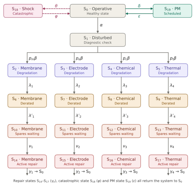
Figure 2.
State-transition diagram of the extended 20-state PEM electrolyser model with the transition rate marked on every edge (α, pjβ, λk, λ′k, νk, γk, δ, ε, θ, φ); dashed arrows denote the rare catastrophic-shock branch.
Figure 2.
State-transition diagram of the extended 20-state PEM electrolyser model with the transition rate marked on every edge (α, pjβ, λk, λ′k, νk, γk, δ, ε, θ, φ); dashed arrows denote the rare catastrophic-shock branch.
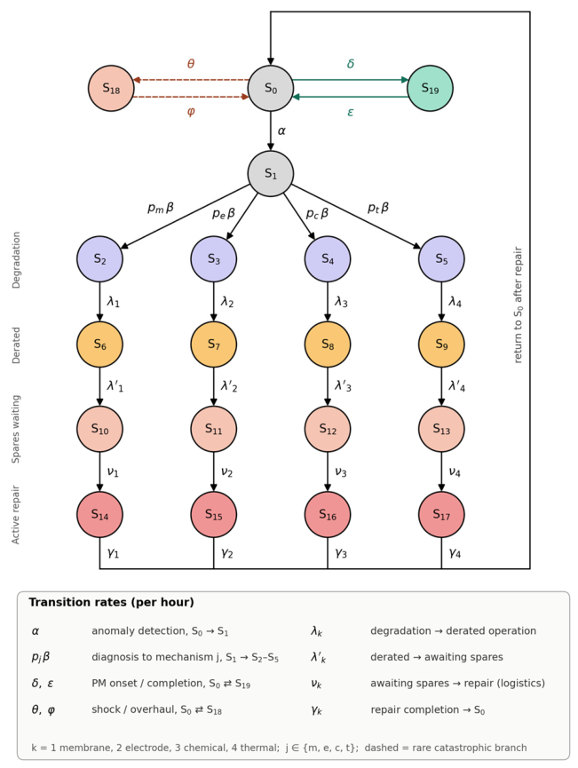
Table 1.
AVAILABLE RATES (FROM [35], /HOUR UNLESS NOTED).
Table 1.
AVAILABLE RATES (FROM [35], /HOUR UNLESS NOTED).
| Parameter | Value | Source / meaning |
| α | 0.00015 | Rate of PEM degradation onset (available, [35]) |
| β | 1.5 | Rate of diagnostic inspection (available, [35]) |
| λ1 (mem.) | 0.002 | Degradation→derated rate (available, [35]) |
| λ2 (elec.) | 0.04 | Degradation→derated rate (available, [35]) |
| λ3 (chem.) | 0.025 | Degradation→derated rate (available, [35]) |
| λ4 (therm.) | 0.001 | Degradation→derated rate (available, [35]) |
| γ1 (mem.) | 0.0024 | Repair→operative rate (available, [35]) |
| γ2 (elec.) | 0.0023 | Repair→operative rate (available, [35]) |
| γ3 (chem.) | 0.0025 | Repair→operative rate (available, [35]) |
| γ4 (therm.) | 0.002 | Repair→operative rate (available, [35]) |
| pm, pe, pc, pt | 0.3, 0.4, 0.2, 0.1 | Diagnostic classification probabilities (available, [35]) |
Table 2.
ASSUMED RATES FOR THE NEWLY INTRODUCED STATES (/HOUR UNLESS NOTED).
| Parameter | Assumed value | Rationale |
| δ | 0.00139 (1/720 h) | Scheduled PM interval ≈ monthly — typical industrial PM cadence |
| ε | 0.25 (1/4 h) | PM duration ≈ 4 h — illustrative, per routine-maintenance practice |
| θ | 0.00005 (1/20,000 h) | Catastrophic shock — rare-event rate consistent with shock-competing multi-state models [13] |
| φ | 0.00417 (1/240 h) | Catastrophic overhaul ≈ 10 days — illustrative major-repair duration |
| λ′1, λ′2, λ′3, λ′4 | 0.010, 0.050, 0.030, 0.008 | Derated→waiting progression rates — assumed proportional to base λk |
| ν1, ν2, ν3, ν4 | 0.0208, 0.0417, 0.0278, 0.0417 | Waiting→repair (logistics delay) rates — 1–2 day spares lead time, per ALDT guidance [36] |
Table 3.
EXTENDED STATE-SPACE DEFINITION.
| State | Description | Category |
| S0 | Operative — baseline healthy condition | Normal |
| S1 | Disturbed — automated diagnostic in progress after an anomaly is flagged | Diagnostic |
| S19 | Preventive maintenance — scheduled intervention, independent of anomaly detection | Scheduled |
| S18 | Catastrophic / common-cause shock — sudden failure bypassing the gradual path | Rare event |
| S2 / S3 / S4 / S5 | Membrane / electrode / chemical / thermal degradation classified by diagnostics | Degradation |
| S6 / S7 / S8 / S9 | Derated operation — reduced current density, partial H₂ output, per mechanism | Derated |
| S10 / S11 / S12 / S13 | Awaiting spares — logistics / administrative delay, per mechanism | Logistics delay |
| S14 / S15 / S16 / S17 | Active repair / replacement in progress, per mechanism | Repair |
Disclaimer/Publisher’s Note: The statements, opinions and data contained in all publications are solely those of the individual author(s) and contributor(s) and not of MDPI and/or the editor(s). MDPI and/or the editor(s) disclaim responsibility for any injury to people or property resulting from any ideas, methods, instructions or products referred to in the content. |
© 2026 by the authors. Licensee MDPI, Basel, Switzerland. This article is an open access article distributed under the terms and conditions of the Creative Commons Attribution (CC BY) license (http://creativecommons.org/licenses/by/4.0/).
Copyright: This open access article is published under a Creative Commons CC BY 4.0 license, which permit the free download, distribution, and reuse, provided that the author and preprint are cited in any reuse.