
Submitted:
23 September 2026
Posted:
29 September 2026
You are already at the latest version
Abstract
The objective of the paper is to offer a complete model for inflation avoiding singularities. It is essentially a revision of the ideas presented in [14,15]. Our model starts with a collapsing object, e.g. a star or a collection of stars, which via a bounce and a succeeding inflation and continued expansion gives output parameters agreeing with all observed cosmological parameters as well as continuously providing a well defined frame of rest. The method of our investigation is a computer simulation of a collapse-bounce-inflation-expanding- Friedmann universe. The results of the model are output parameters agreeing with the observed cosmological parameters, the power index of the CMB, the running of the power index, the present Hubble constant, dark energy density, matter and dark matter density and the radiation density.
Keywords:
cosmology
; theory
; frame of reference
; inflation
; dark energy
; methods: numerica
I. Introduction
As a starting point for our universe a number of different inflation scenarios have been suggested, see e.g. Porcelli and Scibona [1] including bounce inflation e.g. Kaur et al. [4] and Bozza [5]. The inflation is thought to be driven by the energy density of a vacuum energy (zero point energy fluctuations) field. It is generally assumed that the vacuum energy field can be modeled by a scalar field. The only observed fundamental scalar field is the Higgs field with the associated Higgs particle. While the Higgs field could be inflation driving, see Javier Rybio [2] and Rinaldi [3], there are many other possibilities. Generally inflation scenarios leave one or more of the following questions unanswered,
- 1.
- The physics and origin of the pre-inflation universe
- 2.
- The isotropy-homogeneous problem, which is translated to a pre-inflation period
- 3.
- Establishment of a global frame of rest at the end of inflation.
For the universe to be globally isothermal, the standard inflation scenario requires that the pre-inflation universe must have been thermalized for the scalar field to be globally isotropic and homogenous. For general initial conditions see Goldwirth and Piran [6]. These conditions are however not sufficient to establish a preferred global frame of rest at the end of inflation. Particle nucleation will need interaction with already existing particles, see e.g. Garriba et al. [7]. The standard "cold" inflation would have dispersed all particles that existed before inflation. Since both the scalar field and the de Sitter space are Lorentz invariant there is no trace of a preferred reference frame, see "How does inflation isotropize the Universe?" Annino et al.[13]. In contrast to most theories the "warm inflation" suggested by Berera [8], Berera and Fang [9] and Graham and Moss [12] is associated with a thermal heat bath which defines a preferred global restframe. This still leaves the question of the initial establishment of the preferred global restframe and the nature of the pre-inflation universe unanswered. Bounce theories are generally incomplete and/or based on nonstandard physics, e.g. string theories or modified general relativity. Brandenberger and Peter give a thorough review of the progress and problems with bouncing cosmologies. [32].
Based on our lack of understanding the physics of vacuum fluctuations we suggested [14,15] a different possibility that by introducing an upper density limit where further increase in relativistic energy density would transit to vacuum energy density, a space or central region of a stellar object (where the density is more or less isotropic) collapsing towards a black hole would bounce into a new inflating space connected to the original space. Such a "baby space", but at a much higher density has been modeled by Alescil et al,[16]. An isothermal and isotropic (due to the upper density limit) heat-bath, defining a frame of rest, will then be maintained throughout the bounce and the following inflation. The scalar energy density first decays rapidly and then leaves a rest known as dark energy driving the present expansion of the universe.
The present work is a revision of our work cited above.
II. The Model
We start the model in a late collapsing phase where all matter has become relativistic and summed with radiation energy density to and a (negative) curvature energy density . As the collapse continues and reaches further increase in will be transferred to (the scalar energy density) and will have as a result that the sum of scalar and relativistic energy density will approach an increase of where a is the scale factor and in time become equal and opposite to the curvature energy density which increases as , which in turn results in a bounce.
Following the bounce the "universe" will, due to the almost constant start to expand nearly exponentially and the relativistic energy decrease. As the temperature falls the vacuum energy becomes "oversaturated" and will, as the sum of relativistic and nonrelativistic thermal energy density develops a gap to the upper density level, start to condense to the thermal rest-frame. The transfer of scalar energy to relativistic energy will therefore begin at a relativistic energy-density somewhat lower than the upper density level resulting in an hysteresis effect, allowing the inflating object to become much larger than the collapsing object, cf "Hysteresis in the Sky" [17]. The rate of transfer must depend on the scalar energy density and the energy density necessary to provide a rest-frame and "condensation nuclei" for . We note that because of the rest-frame requirement there can be no spontaneous decay of . We also assume that the transfer is mediated by the gravitational field such that the rate of transfer depends on the inverse of the Hubble-time. The rate of transfer of scalar energy density to relativistic energy density is then
where is a normalizing energy density constant,
Figure 1.
Curvature radius of the model universe as a function of time. Time and radius where the observed CMB fluctuations were created is noted by the vertical line.
Figure 1.
Curvature radius of the model universe as a function of time. Time and radius where the observed CMB fluctuations were created is noted by the vertical line.
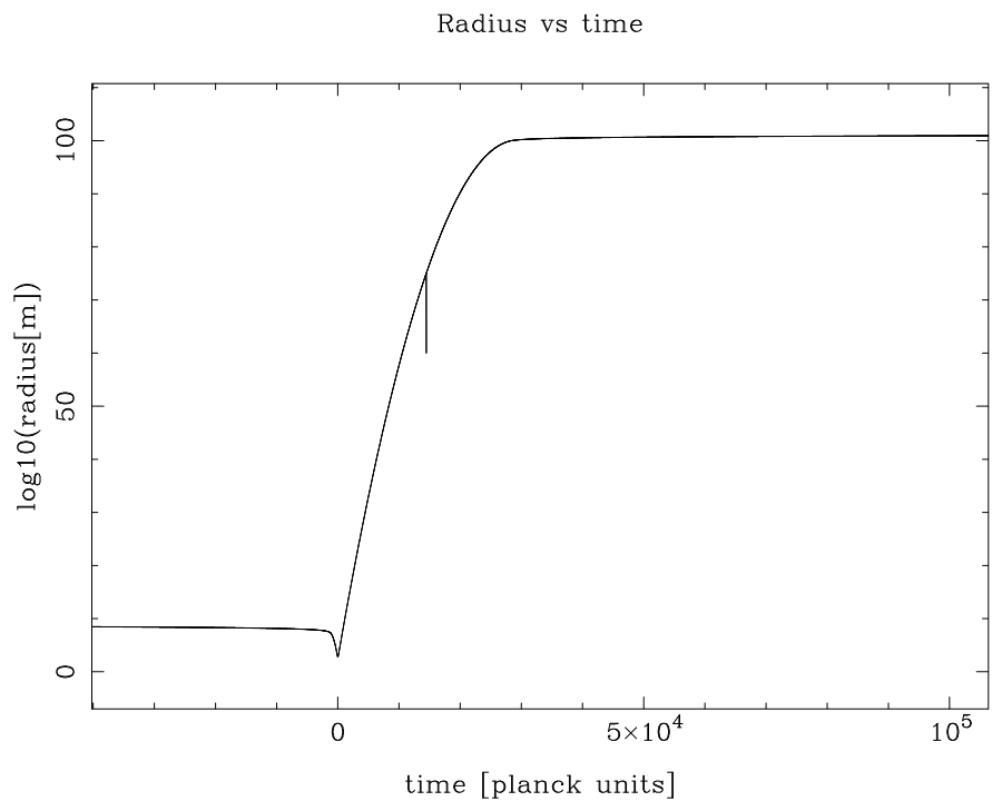
Figure 2.
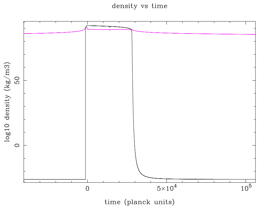
Scalar density (black) and thermal density (red) as a function of time. The time is zero at the bounce. Time and density where the CMB fluctuations were created is noted by the vertical line at which point is and 200 times larger than .
Figure 2.
Scalar density (black) and thermal density (red) as a function of time. The time is zero at the bounce. Time and density where the CMB fluctuations were created is noted by the vertical line at which point is and 200 times larger than .
is determined by the fluctuation amplitude and the spectral power index of the CMB [19]. The quantum density fluctuations are proportional to the density at the time of creation with a wavelength of the size of the event-horizon [14]. This allows the determination of the power index as a function of (comoving) wavelength (Figure 3). is adjusted to give the observed power index at the density the density at which the [18] fluctuations of the CMB were created [14]. The resulting Model running power index becomes The duration of the exponential expansion depends on the gap between and and must be large enough so that the curvature density decreases below the evolving sum of and , if not, the expansion will end and turn into a collapse. values somewhat higher than in the Table 1 below will lead to collapse. determines the rate of transfer of to and later to , and (the photon, the neutrino and the total mass energy density) in proportion and . The condensation temperature for (dark matter), is not known but is here set equal to the baryon condensation temperature. The evolution of curvature fluctuations, important for the formation of mass aggregations, is not presently included in our studies.
With our choice of input parameters in Table 1, the model dark energy density, radiation energy density and CMB power index agree with the observed values [19] and [26]. The exact value of depends on the exact value of the Hubble constant (see Table 2 below).
The model evolution is determined by the Friedman equation. Following the bounce the model enters a period of inflation, or nearly exponential expansion due to the relatively constant . The evolution of the radius is displayed in Figure 1 and the density in Figure 2. As decreases, below the condensation level , transfers very rapidly to , becoming much less than . Already at a time of after the bounce (the end of Figure 2), the scalar density has reached , approaching the standard dark energy density, while the relativistic energy density is allowing for the contracting gravitational force to become dominant. The energy transfer (cf eqn. (1)) becomes exceedingly small at later times so that very quickly become almost "static" and equal to the standard dark energy. The following evolution is then more or less identical to the standard model and is continued until the CMB reaches today’s value.
determines the evolving ratio of to whose sum (at early times) together with determines H. The estimated value of (today’s value of H) differs depending on method of observation see Knox & Millea 2019. We will here adapt the model to the two different estimates of , [28] (supernovae observations) and [19](CMB observations), demonstrating the Hubble tension [24] and [27] which unfortunately cannot be solved by our model.
The condensation of (matter density ) from (relativistic density) at a relevant redshift is adjusted to agree with observations e.g. [19]. Neutrinos are included in .
The speed of sound is cf [11] in ionized plasma is
where is the baryon density and is the E.M. radiation density. and the comoving sound horizon is
where is the scale factor at time t , today’s scale factor and the time when the recombination temperature is reached. A standard baryon fraction is included in our calculations. The sound horizon and the distance produced by the model provides the sound horizon angular size which is required to agree with the value very precisely determined by Planck observations ([19]). The only way to adapt to the planck value in our model is to adjust the effective recombination temperature (), shown in the Table 2, displaying the model adaption to the planck and the supernovae result.
III. Discussion
Singularities in relativity are problematic for a number of reasons see e.g. Stoica [20]. If singularities for any reason are excluded in a collapsing spherical space, the energy density has to increase slower than the curvature density as where a is the scale factor, which in turn either requires a negative pressure or a curvature limit both resulting in a bounce. This possibility was first investigated by Gliner [21] and Sakharov [22]. It was pointed out by Gliner that general relativity is not a closed theory. Citing Gliner "In this sense the general theory of relativity is not a closed theory, and this has been regarded, particularly by Einstein [23] as a serious shortcoming of the theory". Therefore the einstein equations on themselves say nothing about singularities. Only if constraints (e.g. the strong energy condition) are added does singularities become inevitable. We note here that dark energy, the existence of which is strongly supported by the observed accelerated expansion of the universe, and also the hypothesized scalar field [6] in inflation theories break the strong energy condition. We further note that the Schwarzschild solution is constrained to be static, while a static situation might in fact be excluded e.g. due to Hawking radiation and an evolving center as suggested here.
Our model avoids both the initial big bang and the black hole formation singularities. Brandenberger and Mukhanov, [31], [30] avoid singularities in a somewhat similar way. Novello [29] and Brandenberger [32] have made reviews on bouncing cosmologies. We emphasize that our model concerns the evolution of a collapsing central isotropic region of a star or space. It does not concern how or if this collapsing then expanding region is connected to the outer regions of the star or to the geometry of the black hole or a possible wormhole [35] or a possible singularity. We note that both string theory a quantum loop theory suggest that singularities don’t exist in "real physics". If a bounce actually occurs, it seems a wormhole or "baby universe" [16] must develop, since if it bounced back to the original space it would appear as a white hole which has never been observed.
The outer parts of the star or parts which in a possible fracturing process don’t reach the inflation densities will become vanishingly small compared to the inflating parts.
The model assumes a smooth density distribution in e.g. a stellar center, consisting of a soup of relativistic particles approximately in equilibrium. The "boiling process" when the density reaches the upper limit may cause turbulence creating scalar particles. The model assumes that all particles including the scalar are boiled off so that the total number of particles diminishes as the space shrinks. A number of workers have tried to understand the difficult problems with unitarity in gravitational physics e.g. [33] and [34]. Succeeding the bounce, space and particle numbers expand leading to enormous increase in entropy. Inflation models suggest that "zero point quantum fluctuations" get stuck and become real in the expanding space and in turn transferred to particles created by the decaying scalar field. Thus the new information given to the created particles is created by the random number generation of the quantum scalar field. Our model requires, this process to go backwards. I.e. information stored in particles in the collapsing space must be absorbed into zero-point fluctuations of the scalar field.
As is the case with many complex microscopic processes in phase-transitions (e.g. the boiling, the condensation and the ice formation of water) our model suggests that the macroscopic evolution of a "bounce" can be described very simply.
If the type of bounce suggested here actually exist the general image is that of spawning universes which succeeding spawning are left to die in a slow inflation to oblivion, not unlike biological life.
Acknowledgments
My work was supported by the Department of Space, Earth and Environment at Chalmers university of technology. I’m grateful for help given by the staff at the Onsala Observatory. I thank Å. Hjalmarson for reading and commenting the manuscript.
Appendix A. Parameters
- 1.
- , scalar density
- 2.
- , relativistic density
- 3.
- , total matter density
- 4.
- , sum of relativistic and non-relativistic densities
- 5.
- , dark matter density
- 6.
- , radiation density
- 7.
- , baryon density
- 8.
- , neutrino density
- 9.
- , upper density limit
- 10.
- , scalar energy condensation level
- 11.
- , normalizing density
- 12.
- , effective recombination temperature
- 13.
- , last scattering surface
- 14.
- , comoving distance to LSS
- 15.
- , comoving sound horizon
- 16.
- , viewing angle of the sound horizon
- 17.
- , the time dependent Hubble "constant"
- 18.
- , the Hubble constant of today
References
- Fernando Porcelli and Giancarlo Scibona, Large-Scale Structure Formation via Quantum Fluctuations and Gravitational Instability. International Journal of Geosciences, Vol.5 No.6(2014), Article ID:46224,23 pages.
- Javier Rubio. Higgs inflation. Front. Astron. Space Sci., 22 January 2019. [CrossRef]
- M. Rinaldi, Higgs dark energy arXiv:1404.0532 [astro-ph.CO] (2015). [CrossRef]
- Manjeet Kaur,Debottam Nandi, Debajyoti Choudhury, and T. R. Seshadri Universe bouncing its way to inflation arXiv:2302.13698 (2024). [CrossRef]
- Valerio Bozza Cosmological perturbations in bouncing cosmologies and the case of the Pre-Big Bang scenario arXiv:2207.06068 (2022). [CrossRef]
- Dalia S. Goldwirth and Tsvi Piran.(1992). INITIAL CONDITIONS FOR INFLATION, Physics Reports, Volume 214, Issue 4, May 1992. [CrossRef]
- Jaume Garriga, Sugumi Kanno, Misao Sasaki, Jiro Soda, Alexander Vilenkin Observer dependence of bubble nucleation and Schwinger pair production arXiv:1208.1335 [hep-th]. [CrossRef]
- A. Berera. Warm Inflation. Phys. Rev. Lett. 75, 3218 (1995). [CrossRef]
- Arjun Berera and Li-Zhi Fang.(1995). Thermally Induced Density Perturbations in the Inflation Era. Phys. Rev. Lett. 74, 1912, Published 13 March 1995. [CrossRef]
- Lloyd Knox. and Marius Millea. The Hubble Hunter’s Guide astro-ph>arxive:1908.03663 (2019). [CrossRef]
- Edward L Wright Acousitc waves in the early universe J. Phys.: Conf. Ser. 118 012007 (2008). [CrossRef]
- Chris Graham and Ian G Moss. Density fluctuations from warm inflation. arXiv:0905.3500 [astro-ph.CO] (2009). [CrossRef]
- Peter Anninos, Richard A. Matzner, Tony Rothman, and Michael P. Ryan, Jr. (1991) How does inflation isotropize the Universe? Phys. Rev. D 43, 3821, Published 15 June 1991. [CrossRef]
- G. Rydbeck.(2009). On the possibility of a maximum fundamental density and the elimination of gravitational singularities arXiv:0908.2534v2 [astro-ph.CO] 14 Oct 2009. [CrossRef]
- G. Rydbeck, (2023). Bounce inflation with a conserved frame of rest 2023arXiv230413577R. [CrossRef]
- Emanuele Alesci1, Sina Bahrami and Daniele Pranzetti, 2020. An asymptotically de Sitter Universe inside a Schwarzschild black hole arXiv:2007.06664v2. [CrossRef]
- Sayantan Choudhury and Shreya Banerjee.(2016). Hysteresis in the Sky. arXiv:1506.02260v3 [hep-th] 8 Mar 2016. [CrossRef]
- Martin White, Douglas Scott, and Joseph Silk. (1994). ANISOTROPIES IN THE COSMIC MICROWAVE BACKGROUND, Annu. Rev. Astron. Astrophys. 1994. 32: 319-70.
- Planck Collaboration 2019, Planck 2018 results. X. Constraints on inflation. arXiv:1807.06211v2 [astro-ph.CO] 2 Aug 2019. [CrossRef]
- O. C. Stoica. (2012). An Exploration of the Singularities in General Relativity arXiv:1207.5303. [CrossRef]
- Gliner, E.B. Algebraic Properties of the Energy-Momentum Tensor and Vacuum-Like States of Matter. Soviet Physics JETP, 22, 378-382.(1966).
- A.D. Sakharov The Initial Stage of an Expanding Universe and the Appearance of a Nonuniform Distribution of Matter. Soviet Physics JETP, Vol. 22, p.241-.(1966).
- A. Einstein, The Meaning of Relativity, Princeton University Press, 1955, Appendix II.
- Marc Kamionkowski, Adam G. Riess, The Hubble Tension and Early Dark Energy. arXiv:2211.04492 (2022). [CrossRef]
- H.E.S. Velten, R.F. vom Marttens, W. Zimdahl. Aspects of the cosmological "coincidence problem". arXiv:1410.2509v1 (2014). [CrossRef]
- Abhijit Saha and Lucas M. Macri, The Hubble Constant from Supernovae. Handbook of Supernovae, ISBN 978-3-319-21845-8. Springer International Publishing AG, 2017, p. 2577 (2017).
- J. L. Bernal, L. Verde, and A. G. Riess, Journal of Cosmology and Astroparticle Physics 2016, 019 (2016), The trouble with H0 arXiv:1607.05617 (2016).
- An updated measurement of the Hubble constant from near-infrared observations of Type Ia supernovae Lluis Galbany, Thomas de Jaeger, et.al.. arXiv:2209.02546v2 [astro-ph.CO] 18 Sep 2023. [CrossRef]
- M. Novello, S.E.Perez Bergliaffa, . Bouncing Cosmologies. Phys.Rept.463:127-213, (2008). arXiv:0802.1634 [astro-ph]. [CrossRef]
- V. F. Mukhanov and R. H. Brandenberger, “A Nonsingular universe,” Phys. Rev. Lett. 68, 1969 (1992).
- R. H. Brandenberger, V. F. Mukhanov and A. Sornborger, “A Cosmological theory without singularities,” Phys. Rev. D 48, 1629 (1993) [arXiv:gr-qc/9303001]. [CrossRef]
- Bouncing Cosmologies: Progress and Problems Robert Brandenberger and Patrick Peter, (2016) arXiv:1603.05834v2. [CrossRef]
- Unitarity Problems for an Effective Field Theory Description of Early Universe Cosmology Robert Brandenberger, Vahid Kamali. arXiv:2203.11548 (2022). [CrossRef]
- AN INTRODUCTION TO BLACK HOLES, INFORMATION, AND THE STRING THEORY REVOLUTION The Holographic Universe Leonard Susskind, James Lindesay World Scientific Publishing Co. Pte. Ltd.(2005).
- Humanly traversable wormholes Juan Maldacena and Alexey Milekhin PhysRevD.103.066007 (2021).
Figure 3.
Power index of the CMB fluctuations as a function of inverse wavelength. Wavelength and index where the observed CMB fluctuations were created is noted by the vertical line
Figure 3.
Power index of the CMB fluctuations as a function of inverse wavelength. Wavelength and index where the observed CMB fluctuations were created is noted by the vertical line
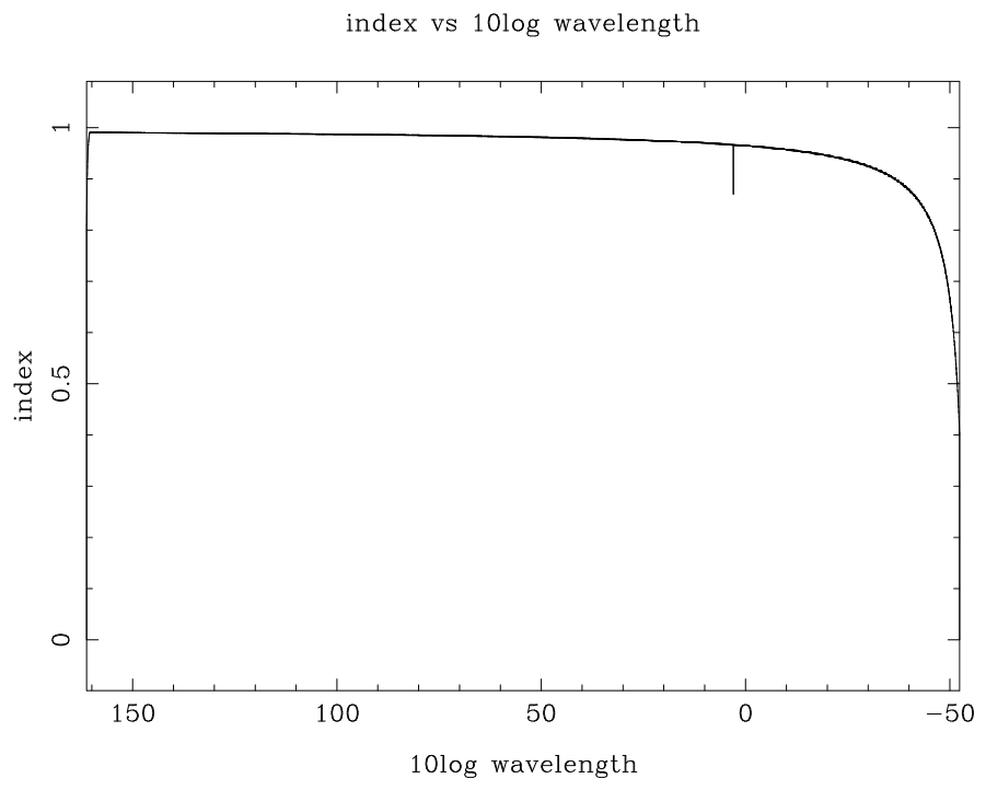

Table 1.
Input densities.
| 1. 2. 3. |
| 2955 | 2.63 | 145.7 | 13985 | 0.5967 | ||||
| 3135 | 2.73 | 141.2 | 13560 | 0.5966 |
Densities are in , temperature in K, distances in , the hubble constant in and angle in degrees. The first two columns are input parameters in the model. is the dark energy, todays value of .
Disclaimer/Publisher’s Note: The statements, opinions and data contained in all publications are solely those of the individual author(s) and contributor(s) and not of MDPI and/or the editor(s). MDPI and/or the editor(s) disclaim responsibility for any injury to people or property resulting from any ideas, methods, instructions or products referred to in the content. |
© 2026 by the authors. Licensee MDPI, Basel, Switzerland. This article is an open access article distributed under the terms and conditions of the Creative Commons Attribution (CC BY) license (http://creativecommons.org/licenses/by/4.0/).
Copyright: This open access article is published under a Creative Commons CC BY 4.0 license, which permit the free download, distribution, and reuse, provided that the author and preprint are cited in any reuse.