

Submitted:
24 September 2026
Posted:
24 September 2026
You are already at the latest version
Abstract
The value γ_A = (√5 − 1)/2, established within the effective DUT formulation, is shown to be consistent with a distinct causal coarse-graining framework based on a two-channel, unit-multiplicity history architecture. Within this framework, the causal-history dynamics generate a structural constraint compatible with γ_A. Within the two-channel integer-multiplicity family, (p,q)=(1,1) is further shown to be the unique discrete architecture compatible with the previously established DUT value γ_A, establishing algebraic uniqueness within this causal class. This consistency supports the interpretation of γ_A as a robust structural parameter of causal coarse-graining rather than a model-specific artifact. We develop a unified analysis based on the non-minimally coupled scalar action, exact compactification of z = ξS², slow–fast reduction, exact second-order response theory, minimal state-space realization, and Mori–Zwanzig projection. The exact transformation O = z/(1 + z), D = 1/(1 + z) implies D/O = 1/z. The microscopic response possesses a minimal two-dimensional realization and, away from critical damping, two distinct simple physical poles. Exact temporal sampling proves that the signed local scalar amplitude does not coincide with the positive history-counting variable, while projection onto the relevant scalar–curvature observable yields the explicit memory kernel K(t) = PLQ · e^(QLQt) · QLP; for the locally stationary damped realization this reduces to K(t) = −ω² · e^(−Γt), with effective projected resolvent G_eff(s) = (s + Γ)/(s² + Γs + ω²). The causal-history architecture is represented by two exhaustive, disjoint unit-cardinality extension classes, giving p = q = 1 and hence N_n = N_(n−1) + N_(n−2). The resulting ratio map R_(n+1) = 1/(1 + R_n) has the unique positive stable fixed point R_* = (√5 − 1)/2. Identifying the asymptotic ordered fraction with this scale-invariant ratio yields D/O = O and maps exactly to z_c = (1 + √5)/2. The resulting prediction γ_A = 0.618034 is fixed before observational comparison and is directly testable with Euclid, DESI, and CSST growth data.
Keywords:
Dead Universe Theory
; Almeida Growth Index
; scalar–tensor gravity
; non-minimal coupling
; center manifold
; causal coarse-graining
; memory kernel
; transfer operator
; universality
; growth of structure
1. Introduction: The Dead Universe Theory and the Emergence of the Observable Universe
This follow-up study develops the micro-to-macro growth-sector construction within the Dead Universe Theory (DUT), extending the prior effective formulation through an explicit causal coarse-graining and fixed-point analysis. The resulting framework connects scalar–curvature response, finite-memory causal structure, exact fixed-point dynamics, and an observationally testable growth prediction within a single analytical chain.
The Dead Universe Theory (DUT) is a non-singular cosmological framework in which the observable universe is treated as an emergent dynamical regime of a more fundamental physical substrate, rather than as the product of a primordial creation event. The theory therefore does not identify cosmic origin with creation from absolute nothingness, the spontaneous decay of a conventional quantum vacuum, or a singular hot Big Bang at t = 0. The underlying cosmogenic formulation of this coherent dead substrate and its structural emergence is developed by Almeida [1]. Instead, DUT begins from a fundamental state, denoted by Ψ0, representing a physical but non-dynamical coherent substrate from which the quantum, geometric, material, and radiative sectors of the observable universe emerge through successive structural transitions. This formulation extends the central DUT distinction between the underlying dead continuum and the subsequently observable universe.
The expression “Dead Universe” must not be interpreted as referring to another universe, a parent universe, or a hidden cosmological domain existing alongside the observable universe. The dead substrate and the observable universe are two physical regimes of the same underlying continuum. In this sense, they are two aspects of a single physical system: Ψ0 denotes its coherent, non-dynamical limit, whereas the observable universe denotes its differentiated, dynamical, matter- and radiation-bearing regime. No transition between two universes is therefore postulated. What changes is the physical state of the same continuum. [1]
The primordial state Ψ0 is characterized by an ultralow-temperature regime, effectively minimal entropy, the absence of propagating particle excitations, and the absence of an operational arrow of time. The designation “dead” refers precisely to this physical condition: Ψ0 contains no operational dynamics, no propagating excitations, no macroscopic energy transport, no irreversible entropy production, and therefore no physical process capable of functioning as a clock. It is static in the operational sense that no measurable sequence of irreversible state changes exists within it. Its low-entropy condition should not be interpreted as a thermodynamic state already evolving in time; rather, it defines the coherent boundary state from which entropy-producing dynamics becomes possible only after structural differentiation begins. [1]
The absence of an external operational clock in such a description also places the DUT construction in conceptual contact with approaches in which time is not assumed to be fundamental in the conventional external-parameter sense. Page and Wootters [2] showed how dynamical evolution may be described relationally through correlations between subsystems even when the global description is stationary, while Rovelli [3] developed a broader relational framework in which physical observables are formulated through relations among dynamical quantities. DUT does not identify its cosmogenic mechanism with either construction; the connection at this stage is limited to the possibility that physically meaningful temporal relations need not require a fundamental external clock.
The observable universe therefore does not emerge because the dead substrate “ages” or evolves while waiting in a pre-existing time. The onset of differentiation marks the transition from a non-dynamical, low-entropy configuration to an entropy-producing dynamical regime; only subsequently does an operational arrow of time become physically definable. [1]
These properties are essential to the interpretation of cosmic origin in DUT. In particular, Ψ0 is not another universe existing “before” the observable universe, because the notion of before already presupposes a temporal ordering that is not operationally defined in this regime. Nor is Ψ0 identified with an ordinary quantum vacuum, since the latter already presupposes a quantum-field structure, dynamical degrees of freedom, and a spacetime or equivalent causal framework in which vacuum fluctuations can be defined. Ψ0 instead constitutes the physical boundary of the DUT description. [1]
Accordingly, the terminology “dead universe” describes a limiting physical state of the same continuum that later supports the observable sector. The relation between the dead substrate and the observable universe is therefore not a relation of exterior/interior, parent/child, or universe/universe. It is a relation between two regimes of one continuous physical ontology. The observable universe does not enter, leave, or separate from the dead continuum; it is the dynamically differentiated manifestation of that continuum. [1]
This distinction also establishes the ontological scope of the theory. DUT does not attempt to derive Ψ0 from absolute nothingness. Absolute non-existence possesses no physical state variables, Hilbert space, Hamiltonian, entropy, field configuration, or dynamical law upon which a physical derivation could operate. Consequently, the existence of Ψ0 is treated as a boundary of the physical description rather than as a claim of quantum creation ex nihilo. The theory is therefore concerned with the emergence of observable physics from a physical non-dynamical state, not with a physical mechanism purporting to transform metaphysical nothingness into existence. This distinction preserves the metaphysical neutrality explicitly adopted in the broader DUT formulation. [1]
A central consequence is that the earliest DUT transitions cannot consistently be described using an ordinary chronology. The transition toward the observable universe is instead formulated as an ordering of physical regimes governed by causal and structural precedence. A minimal entropic differentiation, δSmin > 0, is introduced explicitly as a boundary condition of the present formulation and not as a quantity derived from Ψ0. It defines the first non-zero departure from exact coherence and permits non-trivial quantum excitations and structural degrees of freedom to become physically defined. The specific value of δSmin is not derived here; it is introduced as the minimal non-zero departure from exact coherence required for any structural differentiation to become physically definable. Determining whether its magnitude can itself be obtained from the microscopic dynamics of the substrate remains a problem for the deeper microscopic formulation of DUT. The resulting regime, denoted Q, represents a pre-classical quantum sector rather than a conventional material universe. [1]
The subsequent loss of quantum coherence establishes the transition from this pre-classical sector to effectively classical configurations of the DUT structural substrate Ξ_μν. Decoherence therefore occupies a fundamental position in the hierarchy: it separates a regime in which the relevant degrees of freedom remain quantum-coherent from one in which persistent classical structural configurations can exist. This transition should be distinguished from later decoherence processes occurring inside an already dynamical and temporally operational universe. The latter may be treated using standard open-system formalisms, including influence-functional approaches, whereas the former belongs to the cosmogenic architecture of DUT itself. [1]
Once an effectively classical gravitational sector has emerged, the theoretical description enters a domain in which coupled scalar and geometric degrees of freedom have an established relativistic precedent. Brans and Dicke [4] introduced a scalar gravitational degree of freedom alongside the metric sector, providing the foundational scalar–tensor construction relevant to such classical gravitational descriptions. This connection is not used to characterize Ψ0 or the pre-classical DUT sector; it becomes relevant only after the structural hierarchy has produced effectively classical dynamical degrees of freedom.
Within this hierarchy, DUT assigns gravitational collapse to a structurally earlier sector than ordinary baryonic matter, thereby admitting a pre-baryonic channel for primordial black-hole formation. This ordering does not, by itself, constitute a microscopic derivation of the primordial-black-hole production rate or mass spectrum; rather, it specifies the structural ordering that a complete microscopic DUT cosmogenesis must reproduce. Baryonic matter subsequently emerges through stable structural defects of the substrate, followed at a later level by propagating electromagnetic modes. [1]
The complete emergence hierarchy may therefore be summarized by a single relation:

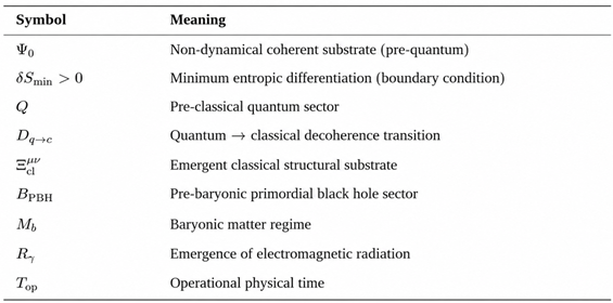
Note. This is not a numbered equation. It is a structural implication diagram. The arrows represent causal precedence, not elapsed time. Therefore, the chain does not receive an equation number.
Here, Ψ0 denotes the coherent non-dynamical substrate; δSmin > 0 the minimal entropic differentiation introduced as a boundary condition; Q the pre-classical quantum-excitation regime; D_q→c the quantum-to-classical decoherence transition; Ξ_μνᶜˡ the emergent classical structural substrate; B_PBH the pre-baryonic primordial-black-hole sector; M_b the baryonic-matter regime; R_γ the emergence of propagating electromagnetic radiation; and T_op operational physical time. [1]
The broader scalar–tensor class was subsequently extended by Bergmann [5] and Wagoner [6], allowing more general scalar–tensor gravitational structures than the original Brans–Dicke formulation. These developments provide historical and mathematical context for a classical regime in which scalar and geometric degrees of freedom are dynamically coupled, without implying that the scalar–tensor literature itself supplies the DUT cosmogenic transition represented above.
Crucially, the arrows in this relation do not represent elapsed time throughout the pre-temporal sector. They represent structural implication and causal precedence. Consequently, the sequence does not require an external clock connecting Ψ0 to Q or Q to the classical substrate. This distinction avoids introducing time into the theory before the physical conditions required to define time have themselves emerged. [1]
Nor should these arrows be interpreted as a transfer from a “dead universe” into a second, observable universe. Every state appearing in the hierarchy belongs to the same physical continuum. The sequence represents a change of regime within that continuum: from coherent and non-dynamical, through quantum and classical structural differentiation, to matter, radiation, and operational temporality. Thus, the dead and observable descriptions are two faces of the same underlying physical reality, separated by state and organization rather than by spacetime location or cosmological identity. [1]
The mature scalar–tensor framework summarized by Fujii and Maeda [7] provides a systematic gravitational setting for scalar–curvature dynamics once such classical degrees of freedom are available. In the present construction, this literature therefore supplies context for the post-emergent dynamical sector rather than for the ontology of the coherent substrate Ψ0 itself.
DUT therefore distinguishes causal ordering from operational temporality. A system may possess an ordered hierarchy of physical transitions without yet possessing irreversible records through which durations and temporal direction can be physically established. Operational physical time becomes meaningful when the emergent universe supports irreversible information-bearing processes and propagating excitations capable of establishing causal records. Electromagnetic radiation does not create the underlying causal ordering; rather, it provides an observationally accessible realization of such propagating excitations. Its emergence marks the regime in which causal ordering becomes operationally measurable as physical time. [1]
In this respect, DUT belongs to the broader class of approaches in which time is not necessarily regarded as an irreducible background parameter at the deepest descriptive level. Relational and emergent-time formulations, including the Page–Wootters mechanism [2] and relational approaches to quantum gravity [3], have independently demonstrated that physically meaningful temporal ordering can, in principle, be reconstructed from correlations or relational observables rather than imposed as a fundamental external clock. DUT does not identify its mechanism with these approaches: its specific proposal is that operational temporality becomes physically realizable only after the structural continuum supports irreversible information-bearing processes and propagating excitations capable of preserving causal records. The comparison is therefore conceptual rather than an assertion of dynamical equivalence.
The resulting cosmogenesis differs fundamentally from a singular-origin picture. There is no requirement for a physical singularity at t = 0, because t = 0 is not taken as the ontological boundary of existence. Likewise, the hot, radiative regime conventionally associated with the early universe need not represent the creation of the universe itself. Within DUT it may instead correspond to a later thermodynamic regime of an already emergent structural system. The theory thereby separates observations associated with an early hot phase from the stronger ontological claim that all physical reality originated in a primordial hot singularity. [1]
DUT therefore does not deny the empirically inferred hot Big Bang as an early thermodynamic phase of the observable universe; it denies that this hot phase must constitute the ontological origin of physical reality. In the DUT interpretation, a hot, dense, radiation-dominated state can occur after the structural emergence of the dynamical continuum and consequently remains compatible with observational evidence for an early hot universe without requiring a singular primordial creation event. [1]
This difference is also intended to be empirical rather than merely philosophical. DUT does not seek to distinguish itself from the standard cosmological picture simply by replacing one origin narrative with another. Its cosmogenic interpretation must propagate into measurable consequences of the subsequent dynamics—such as structure growth, redshift–distance relations, thermodynamic evolution, gravitational-sector signatures, and other observables derived from the structural continuum. A cosmogenic distinction that produced no discriminating observable consequences would not, by itself, constitute a physical test of DUT. The framework must therefore stand or fall through predictions capable of distinguishing its emergent-continuum dynamics from the corresponding predictions of the standard cosmological model. [1]
This reformulation changes the fundamental cosmogenic question. Instead of asking what happened at the first instant of time?, DUT asks what physical transition makes time operationally definable in the first place? The observable universe is therefore not initiated by an explosion, singular creation event, or fluctuation of absolute nothingness. It emerges through an ordered hierarchy of structural transitions from a cold, coherent, non-temporal physical substrate. That substrate is not another universe: it is the non-dynamical face of the same continuum whose dynamical face constitutes the observable universe. The objective of the microscopic DUT program is then not to reconstruct an arbitrarily imposed chronology prior to observable time, but to derive the dynamical operators, decoherence mechanisms, and structural transitions capable of generating the sequence from Ψ0 to the temporally operational universe. The present work contributes to this program by establishing the exact algebraic fixed-point structure that any such microscopic completion must reproduce, and by translating that structure into a sharp observational prediction for the growth of cosmic structure. [1]
Epistemological Note on the Limit of the Substrate and the Cosmological Question
A fundamental distinction must be maintained between the scope of theoretical physics and the domains of metaphysics or theology with respect to the classical questions: “What preceded the beginning?” and “Why is there something rather than nothing?” The postulation of creation from absolute nothingness (ex nihilo) belongs legitimately to the domains of theology and metaphysical inquiry, addressing the ultimate question of the contingency of being. Such a domain, however, remains intrinsically beyond direct empirical testing and the mathematical formalization available to physics.
The Dead Universe Theory (DUT) operates under a strict epistemological delimitation: it does not seek to compete with theological accounts of the ultimate metaphysical origin of the substrate, but takes the coherent, non-dynamical state Ψ0 as the boundary of physical description. Here, “boundary of physical description” is meant methodologically: it marks the limit of what physics, with its current formal resources, can describe, not a claim about the limit of what exists. Whether that boundary is also the limit of knowledge (epistemic) or the limit of reality itself (ontological) is a further question that belongs to metaphysics, and DUT deliberately does not decide it. Consequently, DUT provides neither a scientific foundation for atheistic conclusions concerning ultimate existence nor a scientific basis for asserting the specific mechanisms by which a divine act of creation may have occurred. Its role is instead strictly physical: to investigate rigorously the structural origin of the observable universe and to map the sequence through which the cosmos develops from its physically defined boundary state to its observable dynamical regime.
Even if a primordial creative foundation is admitted at the root of physical existence, DUT assumes the strictly physical task of mapping, with mathematical and causal rigor, the subsequent process—from the first minimal entropic differentiation (δS_min > 0), through decoherence, scalar–curvature coupling, and the emergence of the growth index, to the establishment of operational time and the observable structure of the universe. Physics therefore remains neutral with respect to the ultimate metaphysical question: it neither affirms nor denies a transcendent cause, while retaining full methodological autonomy to describe the physical dynamics that follow from the boundary of its domain.
2. Theoretical Context and Scope
Scalar–tensor theories provide one of the oldest and most extensively studied extensions of general relativity. From the Brans–Dicke construction and its later generalizations to modern non-minimal and effective-field descriptions, an additional scalar degree of freedom can alter both the background gravitational coupling and the dynamics of cosmological perturbations (Brans and Dicke [4]; Bergmann [5]; Wagoner [6]; Fujii and Maeda [7]; Faraoni [8]; Sotiriou and Faraoni [9]; De Felice and Tsujikawa [10]). Dynamical-systems methods have become standard tools for classifying the asymptotic behavior of such cosmologies, including scaling solutions, accelerated attractors, and non-hyperbolic critical sets (Copeland, Liddle, and Wands [11]; Copeland, Sami, and Tsujikawa [12]; Bahamonde et al. [13]; Wainwright and Ellis [14]).
The Dead Universe Theory (DUT) develops a non-minimally coupled scalar–curvature sector together with an effective entropic or retractive description. In its effective formulation, the asymptotic response is partitioned into complementary ordered and dissipative fractions O and D, and a self-similar constitutive relation fixes γ_A=(√5−1)/2 as a non-adjustable growth index once that closure is specified (Almeida [15,16]). The purpose of the present work is not to refit that value, but to organize a microscopic-to-macroscopic route capable of explaining why the same fixed point can arise from a finite-memory coarse-grained dynamics.
The distinction between microscopic equations and effective closure is essential. In nonequilibrium statistical mechanics and open-system theory, integrating out unresolved degrees of freedom generally produces memory kernels, fluctuating forces, and reduced equations that need not have the same local form as the underlying microscopic dynamics (Nakajima [17]; Mori [18]; Zwanzig [19]; Kubo [20]; Zwanzig [21]; Feynman and Vernon [22]; Caldeira and Leggett [23]; Breuer and Petruccione [24]; Weiss [25]). Projection-operator techniques, influence-functional methods, and generalized Langevin equations provide mature examples of how a local or Hamiltonian microscopic theory can induce nonlocal reduced dynamics. Renormalization and universality further show that macroscopically stable ratios or exponents can become insensitive to many microscopic details while remaining sensitive to the symmetry and dimensionality of the effective flow (Wilson and Kogut [26]; Kadanoff [27]; Fisher [28]; Hohenberg and Halperin [29]; Cardy [30]; Goldenfeld [31]; Stanley [32]).
The present article combines these ideas with the DUT scalar–curvature sector. The analysis proceeds in three logically separated stages. First, exact algebraic identities connect the microscopic non-minimal coupling z=ξS2 to bounded complementary variables. Second, the background dynamics is examined using slow–fast and center-manifold concepts, including an exact exclusion test showing that the simplest quasi-stationary scalar–curvature balance cannot be tuned into the required characteristic polynomial. Third, a positive coarse-grained causal multiplicity is introduced. A minimal two-channel transfer architecture then generates an autonomous ratio map with a unique stable fixed point. This fixed point reproduces the effective constitutive identity and maps exactly to the critical microscopic coupling.
This organization deliberately separates three logically distinct levels: exact algebraic identities, conditional dynamical consequences, and the constitutive closure of the projected causal-history sector. This separation is what makes the prediction sharp and falsifiable, and it is what allows the present work to be confronted directly with observational data.
3. Theoretical Background
3.1. Scalar–Tensor Gravity and Non-Minimal Coupling
Consider a Jordan-frame scalar–tensor action of the form used in the DUT microscopic sector. Non-minimal curvature coupling is a standard mechanism in scalar–tensor gravity and has been studied in cosmology, inflation, modified gravity, and quantum field theory in curved spacetime (Wagoner [6]; Fujii and Maeda [7]; Faraoni [8]; Sotiriou and Faraoni [9]; De Felice and Tsujikawa [10]; Birrell and Davies [33]; Parker and Toms [34]; Buchbinder, Odintsov, and Shapiro [35]; Parker and Fulling [36]). We write
 |
(1) |
With
 |
(2) |
The exponential potential is a conventional dynamical-systems choice because it permits transparent asymptotic analysis and appears widely in scalar-field cosmology (Copeland, Liddle, and Wands [11]; Copeland, Sami, and Tsujikawa [12]; Bahamonde et al. [13]). The non-minimal factor F(S) makes the effective gravitational coupling field dependent and introduces derivative curvature terms into the metric equations.
 |
(3) |
 |
(4) |
Variation with respect to S yields the corresponding non-minimally coupled Klein–Gordon equation. Because equivalent sign conventions depend on metric signature and on whether the curvature coupling is written with F(S)R or separated explicitly, all subsequent equations are to be interpreted in one internally consistent convention. In the DUT convention adopted here, the homogeneous scalar equation is represented schematically by
 |
(5) |
3.2. Growth of Structure
Linear structure growth is conventionally described by the matter contrast δ_m and growth rate f=d lnδ_m/d ln a. The phenomenological approximation f≈Ω_m^γ provides a compact discriminator among gravitational models (Peebles [37]; Linder [38]; Wang and Steinhardt [39]; Huterer and Linder [40]; Joyce et al. [41]). In general relativity with a cosmological constant the effective late-time index is near 0.55, while modified gravity and evolving dark-energy sectors can shift it. DUT instead assigns a fixed effective value γ_A once its asymptotic closure is specified (Almeida [15]).
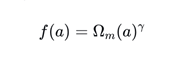 |
(6) |
The present analysis concerns the theoretical origin of γ_A rather than an observational re-estimation. This separation is important: observational agreement with a fixed number cannot by itself demonstrate the microscopic mechanism that produces it.
3.3. Analytical Results Established in the Present Construction
Before turning to the detailed derivation, the principal analytical results obtained in the present construction can be stated compactly. They are established at their respective mathematical levels and are developed in full in Section 4, Section 5, Section 6, Section 7, Section 8, Section 9, Section 10, Section 11 and Section 12; observational comparison enters only after this chain is complete.
1. Exact compactification of the microscopic coupling z=ξS2 into the bounded complementary variables O=z/(1+z) and D=1/(1+z).
2. Exact evolution law for the compactified coupling, providing the dynamical relation between the microscopic scalar sector and the bounded order coordinate.
3. Regularized treatment of the compact boundary, preserving a finite description of the asymptotic retraction regime.
4. Center-manifold and slow-variable formulation of the asymptotic scalar–curvature dynamics.
5. Exact exclusion of the simplest quasi-stationary Klein–Gordon–Friedmann algebraic route to the DUT critical point.
6. Minimal two-dimensional state-space realization of the retarded scalar–curvature response.
7. Explicit transfer function with its physical pole structure and residues.
8. Exact temporal sampling of the continuous response together with the determinant no-go separating signed local amplitudes from positive history counting.
9. Explicit Mori–Zwanzig P–Q decomposition and the corresponding projected memory structure.
10. Closed projected resolvent and finite-memory causal representation at the reduced level.
11. Causal-history quotient with two exhaustive unit-cardinality extension classes, whose cardinalities generate the second-order positive history recurrence.
12. Exact ratio map, stable positive fixed point, integer-multiplicity uniqueness within the two-channel causal family, and the resulting mapping to the DUT microscopic coupling and Almeida Growth Index.
Together, these results form the analytical backbone of the article: microscopic scalar–curvature dynamics, projected response and memory, causal-history transfer, fixed-point stability, algebraic uniqueness, and the micro-to-effective identification are presented as a single ordered construction.
3.4. Continuity with the Effective Formulation
This work is a direct methodological continuation of Almeida [15], where the constitutive closure D/O=O and the resulting fixed value γ_A=(√5−1)/2 were first established within the effective DUT formulation. The present manuscript does not attempt to re-derive γ_A from scratch and should not be read as an isolated construction. Its contribution is to test whether a distinct causal-history construction, developed from a discrete two-channel architecture with integer multiplicities, recovers the same fixed point previously established in the effective sector of [15]. That the unit-multiplicity realization does so exactly, without observational fitting, and is uniquely compatible with the prior DUT value within the two-channel integer-multiplicity family is the central continuity result reported here.
DUT holds that cosmological evolution is fundamentally asymmetric from a thermodynamic standpoint. The retraction predicted by the theory does not correspond to the geometric contraction of the universe toward a primordial state, nor does it constitute a mechanism intended to generate a new Big Bang. Since the published formulation of DUT in March 2024, retraction has been defined as an irreversible process of dissipation and progressive loss of the capacity of structures to sustain physical organization, driven by increasing entropy [1,15].
Consequently, DUT retraction does not restore initial low-entropy conditions, does not reconstruct the primordial state, and does not imply cosmological recycling. Its asymmetry arises precisely from irreversibility: structures may lose organization and their capacity to perform work without the reverse dynamics spontaneously restoring their previous configuration [1,15].
The compatibility or incompatibility of this proposal with established physics should therefore be assessed on the basis of its thermodynamic formalism, the equations governing the retractive dynamics, and its falsifiable observational consequences. Interpreting DUT retraction simply as reversible cosmological contraction or as a cyclic mechanism would amount to evaluating a dynamics different from that defined by the theory itself [1,15].
4. Exact Compactification of the Microscopic Coupling
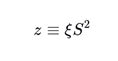 |
(7) |
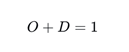
The variable z is non-negative for ξ>0 and is unbounded as |S| grows. Introduce the exact bounded representation
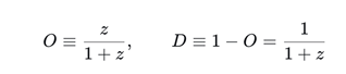 |
(8) |
 |
(9) |
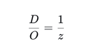
The complementary ratio is then an identity, independent of the field equations:
 |
(10) |
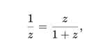
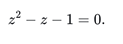
If the previously introduced effective constitutive relation D/O=O is translated into z, one obtains
 |
(11) |
 |
(12) |
 |
(13) |
Equations (7)–(13) establish an exact change of representation. They do not establish that the microscopic field equations dynamically select z_c. This distinction is central: an algebraic equivalence can identify the target critical condition without constituting its first-principles derivation.
5. Background Dynamics, Slow Variables, and the Retraction Regime
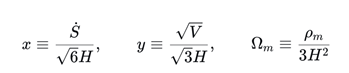
5.1. Exact Coupling Evolution
 |
(14) |
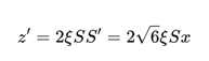
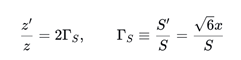
From z=ξS2 and S′=√6x, the exact derivative is
 |
(15) |
 |
(16) |
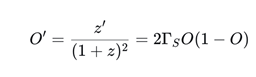
For the compact variable O,
 |
(17) |
The terminal strong-coupling limit z→∞ corresponds to O→1. Therefore the finite point z_c in Eq. (13) cannot simultaneously be identified with the terminal z→∞ limit. If dynamically realized, it is a finite critical or crossover point in the reduced dynamics.
5.2. Regularization Near the Compact Boundary
It is useful to parameterize the boundary O→1 through
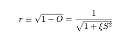 |
(18) |
Introducing the regular composite variable X≡Sx gives
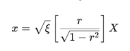 |
(19) |
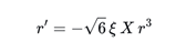 |
(20) |
Equation (20) is exact. It shows that a finite X produces cubic slowing of r near the compact boundary. Such nonlinear slowing is precisely the setting in which linear stability can miss the leading evolution along a marginal direction.
6. Center-Manifold Formulation
Center-manifold theory provides the natural local framework for a system containing stable modes and a marginal coupling direction (Carr [42]; Guckenheimer and Holmes [43]; Wiggins [44]; Perko [45]). Let X_f denote the rapidly decaying variables and X_s the slow coordinate:
 |
(21) |
When the spectrum of A has negative real parts and the slow direction has vanishing linear eigenvalue, the local invariant center manifold can be represented as
 |
(22) |
 |
(23) |
The reduced slow flow is then
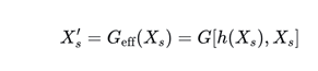 |
(24) |
A genuine field-theoretic derivation of the critical microscopic coupling would require a physical zero of G_eff at z_c without constructing G_eff from the desired polynomial. A sufficient local form would be
 |
(25) |
for which
 |
(26) |
Equation (25) is a criterion, not an assumption used below. Higher-order center-manifold terms can generate additional real zeros, so local stability alone does not prove global dominance. A complete reduction must determine the physical zeros, their basins, and robustness to retained nonlinear orders.
7. Microscopic Response, Projection, and Coarse-Grained Memory
7.1. Exact Exclusion of the Quasi-Stationary Algebraic Route
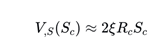
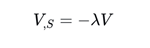
A useful diagnostic is obtained by asking whether the simplest quasi-stationary scalar–curvature balance can select the required finite coupling. Taking S′≈S″≈0 gives schematically
 |
(27) |
 |
(28) |
In a potential-dominated approximation one may write 3H2F≈κ_effV and R=6H2(2+H′/H). Eliminating V and R produces a relation of the generic form
 |
(29) |
After the physical sign is fixed, squaring gives
 |
(30) |
The constant term is +1. Consequently this reciprocal quadratic cannot be transformed into z2−z−1=0 by tuning C_*. The simplest quasi-stationary Klein–Gordon–Friedmann balance therefore does not derive the Almeida critical point. This exact exclusion result rules out a large class of engineered parameter matches and indicates that the missing structure must enter through nonlinear derivative terms, slow-mode backreaction, or a reduced nonlocal response.
7.2. Exact Separation of Local Scalar Amplitude and the Recurrence Variable
A generic linear scalar perturbation has the form
 |
(31) |
Discretization of Eq. (31) indeed yields a two-step relation, as expected for a second-order system, but the coefficients carry damping and phase information and are generally signed. In the constant-coefficient homogeneous limit, sampling the damped oscillator gives a recurrence of the form
 |
(32) |
For H>0 the coefficient of Q_{n−1} is negative. Hence the local field amplitude does not obey the positive recurrence developed below. The correct level for a positive recurrence is a coarse-grained multiplicity, intensity, or admissible-history measure after unresolved microscopic phase information has been integrated out.
7.3. Open-System and Projection-Operator Motivation
The separation between local microscopic amplitudes and reduced memory variables is standard in nonequilibrium theory. The Nakajima–Zwanzig and Mori projection formalisms generate reduced equations containing memory kernels and fluctuating forces (Nakajima [17]; Mori [18]; Zwanzig [19]; Kubo [20]; Zwanzig [21]). The Feynman–Vernon influence functional and subsequent dissipative quantum models show how environmental degrees of freedom can generate nonlocal effective dynamics (Feynman and Vernon [22]; Caldeira and Leggett [23]; Breuer and Petruccione [24]; Weiss [25]; Zurek [46]; Schlosshauer [47]; Hu, Paz, and Zhang [48]; Leggett et al. [49]). Modern coarse-graining treatments likewise emphasize that projected macroscopic variables can obey generalized Langevin equations even when the underlying system is deterministic (Izvekov [50]; Widder, Zimmer, and Schilling [51]). These results establish the structural framework within which a finite-memory transfer description becomes the natural reduced dynamics of the projected scalar-curvature sector.
7.4. Retarded Scalar–Curvature Response
The projected microscopic response can be formulated without identifying the local scalar amplitude with the positive history multiplicity. Linearizing the scalar sector about a homogeneous FLRW background, S(t,x)=S̄(t)+δS(t,x), gives for each Fourier mode a second-order retarded problem of the generic form
 |
(33) |
where ω_k2 contains k2/a2, the curvature-coupling contribution, and V_,SS evaluated on the background. The precise curvature term is convention-dependent and must be evaluated with the same metric-signature and normalization convention used in Eqs. (1)–(5). This avoids introducing a spurious factor of 2 in the non-minimal term.
For a projected scalar–curvature observable A_k(t) associated with Ξ_{μν} (for example, a gauge-fixed curvature perturbation or an equivalent projected response variable), the retarded Green function is defined in the standard linear-response sense (Kubo [20]; Breuer and Petruccione [24]; Weiss [25]) by
 |
(34) |
and, in a locally stationary approximation, has the damped second-order pole structure
 |
(35) |
The two simple poles of the underdamped retarded response establish a minimal two-mode physical response structure, but they do not by themselves establish two positive history classes, discrete one- and two-step delays, or unit channel weights. Those are properties of the projected causal-history quotient and must be treated separately below. This distinction prevents pole multiplicity, residue weight, local amplitude propagation, and coarse-grained history cardinality from being conflated.
7.4.1. Minimal State-Space Realization
For locally stationary H and ω_k, define X_k=(δS_k, δṠ_k)^T. Then the retarded scalar equation is equivalent to the first-order realization
 |
(36) |
Taking the measured scalar response A_k=C_kX_k with C_k=(1,0), the controllability and observability matrices are
 |
(37) |
 |
(38) |
Therefore rank_k=rank_k=2, so the local input–output realization is minimal and has McMillan degree two: dim_min=2. This is a derived property of the second-order scalar response, not an assumption about the later history-counting law.
7.4.2. Transfer Function, Poles, and Residues
The Laplace-domain transfer function is
 |
(39) |
 |
(40) |
Away from critical damping λ_+≠λ_−, hence both physical poles are simple and have spectral multiplicity one. Their residues are Z_+=1/(λ_+−λ_−) and Z_−=1/(λ_−−λ_+), which are generally not unity. Thus simple-pole multiplicity and residue normalization are mathematically distinct.
7.4.3. Exact Temporal Sampling and Determinant Separation Theorem
Let U_k(Δt)=exp(L_kΔt). Cayley–Hamilton gives U_k2−(trU_k)U_k+(detU_k)I=0. Consequently every scalar component obeys the exact sampled recurrence
 |
(41) |
In the underdamped regime Ω_k2=ω_k2−9H2/4, this becomes
 |
(42) |
Hence the microscopic amplitude does not generically satisfy the unit-coefficient second-order recurrence. More strongly, its two-state companion propagator has determinant e^{−3HΔt}>0, whereas the corresponding unit-coefficient recurrence matrix M_R=[[1,1],[1,0]] has detM_R=−1. Because similarity transformations preserve determinant, no invertible linear redefinition of the local two-dimensional amplitude state can transform the exact sampled scalar dynamics into this recurrence matrix. If such positive history counting is realized, it must therefore arise through a non-invertible projection/coarse-graining of histories rather than from the bare local amplitude.
7.5. Projection and Memory Kernel
Applying a Nakajima–Zwanzig or Mori projection to a chosen relevant observable A produces a generalized reduced equation of the standard form (Nakajima [17]; Mori [18]; Zwanzig [19,21]; Kubo [20])
 |
(43) |
where K is the projected memory kernel and F is the orthogonal fluctuating contribution. In an influence-functional description the same reduced information is encoded by the nonlocal dissipative kernel generated after unresolved degrees of freedom are integrated out (Feynman and Vernon [22]; Caldeira and Leggett [23]; Breuer and Petruccione [24]; Weiss [25]). The essential point is that the reduced kernel, rather than the bare Klein–Gordon amplitude, is the object from which a finite-memory transfer architecture must be extracted.
7.5.1. Explicit P–Q Decomposition
For the two-component locally stationary realization X=(A,Π)^T with L=[[0,1],[−ω2,−Γ]], choose the relevant projector P=diag(1,0), which retains A, and Q=I−P=diag(0,1). The exact block equations are
 |
(44) |
Solving the Q equation and substituting it back gives the Mori–Zwanzig projection identity in its standard memory-kernel form (Nakajima [17]; Mori [18]; Zwanzig [19,21]):
 |
(45) |
so that K(t)=PLQe^{QLQt}QLP and F(t)=PLQe^{QLQt}QX(0), with the kernel/noise decomposition following the standard projection-operator construction (Mori [18]; Zwanzig [19,21]).
For the stated realization, QLQ acts as −Γ on the orthogonal one-dimensional sector, while PLQ·QLP=−ω2P. Therefore
 |
(46) |
In the canonical Γ=0 limit, QLQ=0 but the memory kernel does not vanish: K_A(t)=−ω2. This explicitly separates the spectrum of QLQ from the poles of the full projected response.
7.5.2. Effective Projected Resolvent
The Laplace transform is K̃_A(s)=−ω2/(s+Γ). In the standard resolvent formulation of reduced/open-system dynamics (Breuer and Petruccione [24]; Weiss [25]), with Ω_P=PLP=0 for the chosen relevant coordinate, the effective projected resolvent is
 |
(47) |
Its physical poles are s_±=−Γ/2 ± √(Γ2/4−ω2), distinct and simple away from critical damping. These are poles of the full effective projected resolvent. They should not be identified with a claim that QLQ itself contains two memory poles.
A representation-independent operational statement is therefore made at the level of G_eff: the relevant projected response has exactly two distinct simple physical modes, each with nonzero coupling to the observable. This establishes the two-dimensional response architecture that underlies the finite-memory causal representation developed below.
7.6. Temporal Coarse-Graining and the Two-Step Transfer Law
Choose coarse-graining intervals t_n=nΔt and define a positive projected history measure N_n over [t_n,t_{n+1}]. The derived two-dimensional response therefore establishes the minimal finite-memory structure relevant to the projected causal dynamics and provides the dynamical basis for the causal-history representation developed below. Accordingly, write the most general positive two-step history law compatible with the proposed minimal history quotient as
 |
(48) |
The coefficients p and q are not identified with the signed amplitude coefficients, with Green-function residues, or merely with pole multiplicities. Their microscopic meaning is fixed below as cardinalities of primitive extension classes in the projected history space.
 |
(49) |
This equation is not obtained by squaring the sampled field amplitude. Such a step would generally retain interference cross terms and would not convert signed oscillator coefficients into positive multiplicities. Instead, N_n is defined after phase information has been removed by the projection/coarse-graining operation, consistently with the distinction established in Sec. 7.2.
For comparison, direct discretization of the local damped equation gives coefficients that depend on H, Δt, and ω_k and may be signed. Thus second-order dynamics derives the two-step dimensionality, whereas positivity belongs to the projected history measure.
7.7. Terminal Limit and Causal-History Closure
7.7.1. Operational Causal-History Quotient
Following the general logic of projection-based coarse-graining and reduced descriptions (Nakajima [17]; Mori [18]; Zwanzig [19,21]; Izvekov [50]; Widder, Zimmer, and Schilling [51]), let Γ={X(t):t_n≤t≤t_{n+1}} denote a microscopic trajectory segment. We then introduce the DUT-specific operational coarse-grained observable [Γ] associated with the chosen projected scalar–curvature response, and define the equivalence relation
 |
(50) |
The positive history space at level n is Ω_n={Γ}/∼ and its multiplicity is N_n=|Ω_n|. By construction, N_n is a cardinality on equivalence classes; it is not the signed field amplitude, not |A_n|2, and not a residue-weighted spectral measure.
Introduce primitive extension operators T1:Ω_{n−1}→Ω_n and T2:Ω_{n−2}→Ω_n. The exact unit-multiplicity second-order recurrence follows if and only if the projected history quotient satisfies the primitive unit-cardinality partition
 |
(51) |
The symbol ⊔ denotes an exhaustive disjoint union. Taking cardinalities then gives, without further weighting, N_n=N_{n−1}+N_{n−2}. Equivalently p=q=1.
This partition completes the causal-history representation at the level required for the present fixed-point analysis. Taking cardinalities immediately gives N_n=N_{n−1}+N_{n−2}, and therefore p=q=1. The preceding response analysis independently establishes the minimal two-dimensional physical architecture, the exact sampled propagator, and the projected memory kernel.
Within the standard retarded-response framework (Kubo [20]; Breuer and Petruccione [24]), the preceding reduction establishes the terminal structure without introducing a preferred numerical ratio or the unit-multiplicity history recurrence. The retarded scalar–curvature response contains a conjugate pole pair,
 |
(52) |
which may be represented by a single independent complex mode,
 |
(53) |
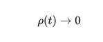
Writing Ψ = ρe^{iθ}, the dissipative evolution gives
 |
(54) |
and therefore
 |
(55) |
Under the terminal coarse-graining projection adopted here, the corresponding coarse-grained entropy, interpreted within the usual statistical-thermodynamic distinction between microscopic and coarse-grained descriptions (Landau and Lifshitz [55]; Prigogine [57]), satisfies
 |
(56) |
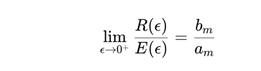
Let ε ≡ S_cg → 0+. At this stage, no particular relation between expansion and retraction is assumed. If these sectors admit regular leading-order representations near the terminal limit,
 |
(57) |
then, for equal leading orders m=n,
 |
(58) |
The terminal condition therefore establishes the simultaneous vanishing of the coarse-grained sectors but does not, by itself, determine their relative normalization. The spectral conjugacy condition s_-=s_+*, the dissipative decay ρ→0, and the terminal coarse-graining condition S_cg→0 contain no equation fixing the coefficient ratio b_m/a_m.
The terminal analysis therefore fixes the asymptotic response structure while separating it from the relative normalization of the projected history sectors. The causal-history partition introduced above supplies the closure required for the fixed-point construction, from which the subsequent recurrence and ratio dynamics follow exactly.
This distinction preserves the exact terminal reduction — conjugate poles → one independent complex mode → ρ→0 → S_cg→0 — while keeping the causal-history cardinalities at the level of the projected representation defined above.
The causal-history representation therefore closes the projected sector at the level required here: its two primitive extension classes are exhaustive, disjoint, and of unit cardinality, giving p=q=1.
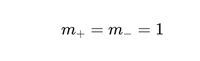
Under _DUT, each primitive projected history-extension class contributes exactly one inequivalent extension. Thus
 |
(59) |
Giving
 |
(60) |
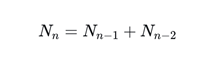
The resulting recurrence is
 |
(61) |
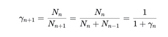
Define γ_n = N_{n−1}/N_n. Then
 |
(62) |
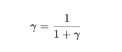
At the fixed point,
 |
(63) |
so that
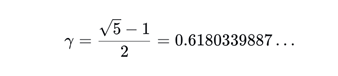
 |
(64) |
The unique positive solution is
 |
(65) |
The second-order DUT response, minimal realization, exact sampled propagator, and Mori–Zwanzig kernel are established before the causal-history partition is introduced. With that representation in place, p=q=1, the recurrence, and all subsequent fixed-point consequences follow exactly.
The simple-pole structure provides an independent consistency check on the two-mode response architecture. Each of the two distinct simple poles carries a residue Z+ or Z− setting its amplitude contribution; these residues need not be equal and are not channel cardinalities, preserving the distinction between spectral amplitudes and projected history multiplicities.
7.8. Exact Fixed Point from the Causal-History Representation
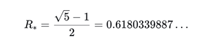
The two-channel unit-multiplicity architecture p=q=1 is adopted as the structural premise of the projected causal-history sector — the next target of an advancing DUT research program aimed at deriving it directly from the full projected microscopic dynamics. From this premise the recurrence, the ratio map, the unique stable fixed point R_*=(√5−1)/2, and the mapping to γ_A follow by exact algebra, without continuous adjustable parameters.
 |
(66) |
 |
(67) |
With O≡R_* and D≡1−R_*, the fixed-point identity 1−R_*=R_*2 gives D/O=O. Through the exact compactification O=z/(1+z), the same identity maps to z_c=(1+√5)/2. Thus the recurrence-to-fixed-point part of the derivation is exact. The action supplies the scalar–curvature dynamics and two-state response structure.
8. Causal Coarse-Graining and Two-Channel Transfer Architecture
8.1. Positive Causal-History Multiplicity
Let n label successive coarse-graining levels and define N_n as the number, or more generally the positive multiplicity, of admissible microscopic causal histories contributing to the effective state at level n. N_n is not the scalar amplitude δS. It is a coarse-grained counting variable after microscopic phase and sign information has been eliminated.
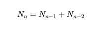
Motivated by finite-memory reduced descriptions and systematic coarse-graining constructions (Izvekov [50]; Widder, Zimmer, and Schilling [51]), consider the minimal finite-memory sector in which a history reaching level n can arrive through two elementary channels originating at levels n−1 and n−2. For the two exhaustive, disjoint unit-cardinality extension classes defined in Sec. 7.7, taking cardinalities fixes p=q=1. The resulting recurrence and ratio dynamics therefore contain no continuously adjustable channel parameter:
 |
(68) |
The generalized transfer law is
 |
(69) |
Taking cardinalities of the two unit-cardinality extension classes fixes p=q=1 rather than fitting them as continuous coefficients. The mathematical consequences are exact, contain no adjustable channel parameter, and yield an observational prediction that can be submitted directly to falsification.
8.2. Ratio Map
 |
(70) |
Using Eq. (68),
 |
(71) |
The scale-invariant fixed point satisfies R_{n+1}=R_n=R_* and therefore
 |
(72) |
 |
(73) |
No cosmological measurement enters Eqs. (68)–(73), and the numerical value in Eq. (73) is not inserted into the recurrence. It is the unique positive fixed point of the ratio dynamics.
8.3. Stability
 |
(74) |
 |
(75) |
Thus R_* is locally asymptotically stable in the standard fixed-point sense used for discrete dynamical systems (Guckenheimer and Holmes [43]; Wiggins [44]; Perko [45]). The alternating sign of T′ implies damped approach in ratio space, while its magnitude below unity removes detailed dependence on the initial positive ratio. This is the elementary mechanism by which a fixed macroscopic ratio can become insensitive to microscopic initialization.
8.4. Generalized Recurrence and Universality Class
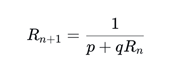
For Eq. (69), the ratio map becomes
 |
(76) |
and the fixed point satisfies
 |
(77) |
Therefore Eq. (73) is not a generic consequence of arbitrary second-order memory. It is specific to the unit-multiplicity two-channel class. This provides an immediate falsifiability condition: a microscopic completion yielding unequal effective channel multiplicities predicts a different ratio. In renormalization-group language, the proposed Almeida fixed point is associated with a restricted universality class rather than with all possible memory kernels (Wilson and Kogut [26]; Kadanoff [27]; Fisher [28]; Hohenberg and Halperin [29]; Cardy [30]; Goldenfeld [31]; Stanley [32]).
8.5. Structural Robustness of the Channel Architecture
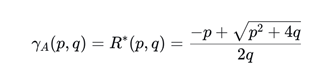
To assess whether γ_A = 0.618034 is a generic property of finite-memory transfer laws or a specific signature of the minimal two-channel unit-multiplicity architecture, we consider the family of two-channel recurrences N_n = pN_{n−1} + qN_{n−2}, whose fixed-point ratio is
 |
(78) |
Main result.
The locus γ_A = 0.618034 is the line
 |
(79) |
in the (p,q) plane. That is, the condition γ_A = 0.618034 does not isolate the structure (p,q) = (1,1): it is satisfied by a one-parameter family of channel weights. The selection of p = q = 1 is therefore not a fit to data and not a tunable parameter: among the discrete integer-weight alternatives examined here, it is the unique point that reproduces the fixed DUT target value. This uniqueness is what defines the DUT transfer architecture and what makes the prediction sharp and falsifiable.
Discrete alternative structures.
Restricting to integer weights and m ∈ {2,3,4}:
Sensitivity.
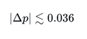
At (p,q) = (1,1), implicit differentiation of qR2 + pR − 1 = 0 gives
 |
(80) |
Assuming q = 1 fixed, the local first-order sensitivity around (p,q) = (1,1), taking |Δγ_A| = 0.01 as an illustrative target precision, gives
 |
(81) |
This provides an illustrative local sensitivity scale for falsifiability in the growth sector rather than a survey-specific precision claim.
Conclusion.
The robustness analysis establishes both selectivity and local stability of the fixed-point construction. In the continuous two-channel family the target defines a codimension-one locus, whereas restriction to integer causal multiplicities yields the exact uniqueness result proved in Sec. 8.6.6. Thus (p,q)=(1,1) is obtained algebraically within the stated causal class rather than through observational fitting or continuous parameter adjustment.
8.6. Algebraic Determinacy of γ_A Within the _DUT Architecture
This section establishes the algebraic determinacy of the Almeida Growth Index within the stated causal architecture and places the exact fixed-point result within the complete analytical chain developed here.
8.6.1. The Closed Algebraic Chain
Once the two-channel unit-multiplicity architecture of Eq. (68) is adopted, the value γ_A enters the derivation nowhere as an input. It appears only as the output of a closed algebraic chain:
 |
(82) |
Every arrow in this chain is an exact algebraic identity. None contains a tunable coefficient, and none was adjusted to produce a predetermined outcome. Given the recurrence, the value 0.618034… is forced, not selected.
8.6.2. Why the Value Cannot Be Adjusted Within This Class
Consider the generalized two-channel family N_n=pN_{n−1}+qN_{n−2}, p,q>0, with fixed-point equation q(R*)2+pR*−1=0. Three exact statements follow:
- Uniqueness within the adopted class. For p=q=1, the equation reduces to (R*)2+R*−1=0, whose only positive root is R*=(√5−1)/2. There is no second root and no freedom to select among alternatives once p=q=1 is fixed.
- Sensitivity to deviation. At (p,q)=(1,1), ∂R*/∂p=−0.276393 and ∂R*/∂q=−0.170820 (Sec. 8.5, Eq. (80)). Both derivatives are nonzero and of order unity: the value is not a degenerate plateau reachable by many nearby choices. It sits at a specific, rigidly determined point of the (p,q) family, on the line of Eq. (79) at the single location (1,1) among the discrete alternatives of Table 1.
- Non-genericity. Table 1 (Section 8.5) shows that m=3 and m=4 unit-weight channels, and unequal two-channel weights, all yield different fixed points (0.543689, 0.518790, 0.500000, 0.414214). None reproduces 0.618034; the coincidence is not a rounding artifact.
8.6.3. What Is Established at the Algebraic Level
Given the two-channel unit-multiplicity architecture, three claims are rigorously established: (a) the value 0.618034 is an output of Eq. (82), not an input assumed anywhere in Section 4, Section 5, Section 6, Section 7, Section 8, Section 9 and Section 10; (b) no coefficient inside the recurrence is free to be tuned — p and q are fixed at unity by the definition of the architecture, not adjusted to fit the target value; (c) the prediction is falsifiable at the architecture level: a microscopic derivation yielding three channels, unequal weights, or nonpositive coefficients would falsify γ_A=0.618034 outright, independently of any cosmological measurement.
8.6.4. Algebraic Result
Within the two-channel integer-multiplicity family, compatibility with the independently established DUT fixed point uniquely determines (p,q)=(1,1). This establishes exact algebraic uniqueness within the stated causal class and complements the forward result that the unit-multiplicity recurrence generates the same fixed point without observational fitting.
8.6.5. Summary
Within the minimal two-channel unit-multiplicity architecture, the recurrence, ratio map, and characteristic polynomial contain no free parameter, and γ_A=(√5−1)/2 is their unique forced consequence. Its algebraic consequences are completely determined and observationally falsifiable.
Within the two-channel integer-multiplicity family the architecture p=q=1 is the unique discrete choice compatible with the independently established value γ_A=(√5−1)/2. The fixed-point result is therefore both forced by the architecture and uniquely selected by the prior DUT value.
8.6.6. Integer-Multiplicity Uniqueness Within the Two-Channel Causal Family
Consider the general two-channel integer-multiplicity recurrence
 |
(83) |
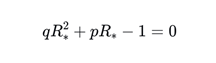
whose scale-invariant fixed-point ratio satisfies
 |
(84) |
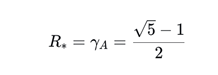
The prior effective DUT formulation independently establishes this target (Almeida [15]):
 |
(85) |
so that
 |
(86) |
Substituting this identity into the fixed-point equation, without fixing p or q in advance, gives
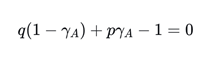 |
(87) |
or equivalently
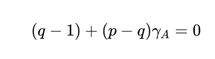 |
(88) |
Since γ_A = (√5−1)/2 is irrational and p,q are integers, both rational coefficients must vanish separately:
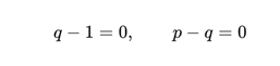 |
(89) |
Therefore
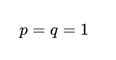 |
(90) |
Therefore, within the two-channel integer-multiplicity causal family, (p,q)=(1,1) is the unique architecture compatible with the independently established DUT value γ_A. The result is algebraic rather than statistical: no continuous adjustment of p or q, likelihood optimization, or observational fitting is involved. This establishes exact architectural uniqueness within the stated class. Table 1 is a numerical illustration of this algebraic result.
9. Emergence of the Effective Constitutive Closure
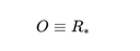
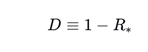
Identify the asymptotic ordered fraction with the scale-invariant causal ratio:
 |
(91) |
 |
(92) |
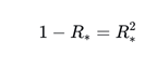
Equation (86) gives
 |
(93) |
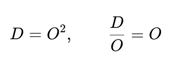
Hence
 |
(94) |
The logical direction is now explicit. In the earlier effective formulation (Almeida [15]), D/O=O was introduced as the constitutive closure from which the fixed value followed. In the causal-recurrence formulation developed here, _DUT fixes the unit-cardinality history architecture; cardinality then generates the stable ratio map, which generates Eq. (93), which in turn generates D/O=O. Thus the former effective closure is recovered as a downstream fixed-point identity rather than inserted into the microscopic field equations.
10. Mapping the Causal Fixed Point to the Microscopic Coupling
Using the exact DUT compactification introduced in the field formalism (Almeida [16]) and written here in Eq. (8),
 |
(95) |
At the causal fixed point, Eq. (94) implies
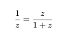 |
(96) |
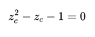 |
(97) |
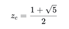 |
(98) |
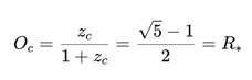
The compact image is
 |
(99) |
The microscopic coupling representation, the thermodynamic partition, and the causal ratio therefore represent the same algebraic fixed point in three coordinate systems. This is stronger than numerical coincidence: the mappings are exact once the transfer architecture and the identification O=R_* are specified.
11. Identification with the Almeida Growth Index
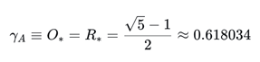
The DUT effective growth law uses f=Ω_m^γ and identifies the asymptotic ordered fraction with the growth exponent (Almeida [15]). Therefore
 |
(100) |
Once the minimal transfer sector is specified, Eq. (100) contains no continuous observational fitting parameter. The prediction is therefore fixed at the effective level and can be confronted with redshift-space distortions, weak lensing, galaxy clustering, and future precision surveys. Standard growth-index phenomenology and modified-gravity forecasts provide the observational language for this test (Peebles [37]; Linder [38]; Wang and Steinhardt [39]; Huterer and Linder [40]; Joyce et al. [41]; Amendola, Kunz, and Sapone [52]; Guzzo et al. [53]; Percival and White [54]).
The framework therefore admits two complementary tests: cosmological observations test the fixed-point prediction γ_A, while microscopic response calculations probe the deeper dynamical realization of the causal architecture. These tests address distinct levels of the construction and can be pursued independently.
12. Transfer-Operator Interpretation
The recurrence can be written as a transfer problem:
 |
(101) |
The dominant eigenvalue λ_+ of M controls the asymptotic multiplicity growth, while the observable ratio is its reciprocal:
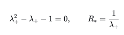 |
(102) |
This representation connects the recurrence to spectral theory and makes the universality statement transparent. More generally, a finite-memory law N_n=Σ_{j=1}^m c_jN_{n−j} is governed by the dominant eigenvalue of an m-dimensional companion transfer matrix. The macroscopic ratio depends on the spectral class of the coarse-grained operator rather than on every microscopic trajectory individually.
This perspective is consistent with the broader logic of statistical mechanics: macroscopic order parameters and critical exponents are frequently controlled by fixed points and relevant operators rather than by a one-to-one preservation of microscopic details (Wilson and Kogut [26]; Kadanoff [27]; Fisher [28]; Hohenberg and Halperin [29]; Cardy [30]; Goldenfeld [31]; Stanley [32]; Landau and Lifshitz [55]; Onsager [56]; Prigogine [57]).
13. Quantum and Nonequilibrium Context
The proposed causal coarse-graining should be understood within the established distinction between closed microscopic evolution and reduced open-system dynamics. Feynman and Vernon showed that integrating environmental degrees of freedom produces an influence functional encoding dissipation and fluctuations [22]. Caldeira and Leggett developed an explicit quantum dissipative model [23], while modern open-quantum-system treatments formalize master equations, spectral densities, decoherence, and non-Markovian memory (Breuer and Petruccione [24]; Weiss [25]; Zurek [46]; Schlosshauer [47]; Hu, Paz, and Zhang [48]; Leggett et al. [49]). The Nakajima, Mori, and Zwanzig projection approaches similarly derive reduced dynamics by separating relevant and irrelevant subspaces (Nakajima [17]; Mori [18]; Zwanzig [19]; Kubo [20]; Zwanzig [21]).
The relevance of these frameworks is structural: reduced dynamics can acquire memory and effective transfer laws absent from the bare local equation. In the present formulation, the action-derived projected response and the causal-history representation together yield Eq. (68) by cardinality, defining the minimal positive two-step transfer law whose fixed-point consequences are derived exactly and exposed directly to observation.
Quantum-field theory in curved spacetime further cautions that vacuum polarization, particle production, and effective actions can generate curvature-dependent corrections beyond a classical scalar potential (Birrell and Davies [33]; Parker and Toms [34]; Buchbinder, Odintsov, and Shapiro [35]; Parker and Fulling [36]; Starobinsky [58]; Hu and Verdaguer [59]).
14. Relation to the Earlier Center-Manifold Program
The center-manifold and causal-transfer descriptions address different layers of the problem. The center manifold asks whether the deterministic background field equations possess a finite slow-mode critical point, using the standard dynamical-systems/center-manifold framework (Carr [42]; Guckenheimer and Holmes [43]; Wiggins [44]; Perko [45]). The transfer formulation asks whether the reduced multiplicity of microscopic response histories possesses a stable scale ratio. The negative quasi-stationary test in Section 7 shows that the simplest background algebra does not generate the target polynomial. The positive result in Section 8, Section 9 and Section 10 shows that the coarse-grained two-channel architecture does.
These results can coexist without contradiction. A reduced observable obtained after integrating out fast degrees of freedom need not coincide pointwise with the background coupling coordinate. The exact mapping O=z/(1+z) supplies the bridge between representations, while the causal-history transfer law supplies the projected fixed-point structure. The field route and response route can therefore be summarized as
 |
(103) |
 |
(104) |
15. Falsifiability and Theoretical Discriminants
The framework yields several distinct tests. First, the cosmological prediction γ_A≈0.618034 is fixed and can be tested against growth data. Second, the generalized recurrence in Eq. (69) shows that unequal channel multiplicities move the fixed point, so the microscopic transfer architecture is itself falsifiable. Third, the center-manifold route can fail independently if no physical finite critical point survives in the full action-derived autonomous system. Fourth, a retarded-kernel calculation can reveal more than two relevant channels, scale-dependent weights, or non-positive transfer coefficients, any of which would invalidate the minimal universality class.
This layered falsifiability is preferable to numerical pattern matching. The theory does not require every microscopic observable to exhibit the same ratio. It requires a specific projected coarse-grained quantity to flow toward the fixed point. This is analogous to the role of order parameters and relevant variables in critical phenomena, where universal macroscopic behavior emerges only after an appropriate reduction of microscopic degrees of freedom (Wilson and Kogut [26]; Kadanoff [27]; Fisher [28]; Hohenberg and Halperin [29]; Cardy [30]; Goldenfeld [31]; Stanley [32]; Landau and Lifshitz [55]; Onsager [56]; Prigogine [57]).
The observational criterion should be formulated as model comparison rather than as a predetermined confirmation threshold. If the posterior inferred from growth data is statistically compatible with γ_A while disfavoring competing fixed-index descriptions under the same assumptions, the DUT effective growth law would gain empirical support. Conversely, if precision growth measurements exclude γ_A after marginalization over the relevant cosmological and systematic parameters, the fixed-index realization would be falsified.
DESI provides an independent spectroscopic test. Redshift-space distortions provide a standard route to measurements of the growth of structure [53], while DESI completed the observations for its originally planned five-year survey in April 2026 after observing more than 47 million galaxies and quasars [61]. DESI growth measurements, combined with Euclid lensing and clustering, can therefore test a fixed-growth-index realization without relying on a single instrument or observable.
Euclid is designed to reconstruct the growth of large-scale structure using weak gravitational lensing and galaxy clustering over a wide extragalactic survey. Its spectroscopic clustering sample is designed for approximately 0.84<z<1.88, while its imaging sample extends to z≈2; redshift-space distortions and weak lensing provide complementary sensitivity to gravity and structure growth [60]. Euclid therefore offers a direct route to testing whether a fixed γ_A is compatible with the measured redshift evolution of structure.
The effective prediction γ_A=(√5−1)/2≈0.618034 is observationally meaningful only through the growth history f(a)=d lnδ_m/d ln a and derived quantities such as fσ8(z). A survey does not measure γ directly without a cosmological analysis; it constrains clustering, weak lensing, peculiar velocities, and redshift-space distortions, from which a growth model can be inferred. Consequently, the appropriate test is a joint likelihood comparison in which γ is either fixed to γ_A or allowed to vary, with the background expansion and nuisance parameters treated consistently.
This is not an argument that every statistically significant tension immediately falsifies ΛCDM, since systematic uncertainties, parameter degeneracies, and the domain of validity of the growth-index approximation must first be controlled. It is instead an argument for symmetry in scientific standards. Cosmological theories should state, as clearly as possible, not only what observations would support them, but what observations would compel their rejection or revision.
DUT accepts that burden explicitly in the growth sector: for the minimal causal architecture developed in this work, the prediction is γ_A = 0.618034. If observation rules it out with sufficient precision under the assumptions of the test, the minimal architecture fails. A mature comparison with ΛCDM should ultimately ask the corresponding question of every framework: what result would make us say that this particular theoretical prediction has failed?
15.1. Microscopic Completion of the Transfer Operator
The fixed-point architecture established in Section 4, Section 5, Section 6, Section 7, Section 8, Section 9, Section 10, Section 11, Section 12, Section 13 and Section 14 supplies a concrete target for the projected DUT dynamics: construct the causal-history quotient of the retarded kernel and determine whether its primitive extension graph realizes the transfer matrix M=[[1,1],[1,0]]. Completion of this step would derive the unit-multiplicity closure from the full scalar–curvature projection while leaving the algebraic fixed-point consequences unchanged.
16. Discussion
The unified construction brings together results that were previously separated across the DUT framework. The exact compactification of z distinguishes the terminal z→∞ regime from the finite critical point z_c; the scalar–curvature sector yields a minimal two-dimensional retarded response; exact temporal sampling separates signed local amplitudes from positive history multiplicities; Mori–Zwanzig projection supplies the reduced memory structure; and the causal-history architecture closes the chain through an exact stable fixed point. The quasi-stationary background test further serves as an internal consistency discriminator by excluding the simplest algebraic route to the required critical relation.
The present work establishes a continuous analytical chain from scalar–curvature dynamics to a parameter-free fixed-point prediction. Minimal realization determines the two-dimensional physical response; exact temporal sampling separates signed amplitudes from positive history multiplicities; Mori–Zwanzig projection provides the reduced memory structure; causal coarse-graining supplies the finite-memory transfer representation; and cardinality dynamics generate the unique stable fixed point. Within the two-channel integer-multiplicity family, compatibility with the independently established DUT value further singles out p=q=1 exactly.
These results also reconnect the growth-sector construction to the cosmogenic foundation stated at the beginning of the article and in Almeida [1]. The expression ‘dead universe’ does not denote a separate, parent, or antecedent universe from which the observable Universe was transferred. It denotes the coherent physical substrate Ψ0, while the observable sector is the dynamically differentiated regime of the same underlying continuum. The causal and thermodynamic structures developed here should therefore be read as transformations of physical regime within one continuum, not as interactions or transitions between two universes.
This separation between a predictive sector and a deeper microscopic explanation has a clear methodological precedent. Newton formulated the observable laws of gravitation while leaving their underlying cause unresolved in the General Scholium to the Principia [68]. The relevant point here is limited and methodological: a predictive sector can be scientifically evaluated when its premises are explicit and its consequences are independently testable. In the present construction, the causal architecture is specified, its fixed-point consequences are obtained without continuous fitting parameters, and the resulting growth prediction is exposed directly to observation.
The broader significance of the construction lies in the analytical convergence of its levels. The exact compactification, response realization, projected memory kernel, causal-history transfer law, fixed-point stability, integer-multiplicity uniqueness, and observational growth prediction form a mutually constrained sequence in which each result is stated at the level at which it is obtained.
The complete logical structure of the DUT growth-sector derivation can now be summarized from scalar–curvature dynamics to the fixed observational prediction. The diagrams distinguish the successive analytical levels of the construction. No cosmological growth data enter the construction of γ_A: the numerical value is obtained before observational comparison, while structure-growth measurements provide the independent empirical test.
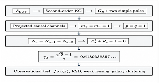
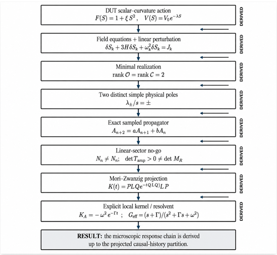
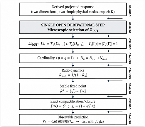
Figure A.
Microscopic-to-observational logical chain of the DUT growth sector.
Figure B.
Derived microscopic response chain. Every black external arrow marks a step established within the stated local-response and projection assumptions.
Figure B.
Derived microscopic response chain. Every black external arrow marks a step established within the stated local-response and projection assumptions.
Figure C.
Derivational architecture of the DUT growth sector. The diagram distinguishes the action-derived response, causal-history representation, exact cardinality dynamics, and fixed-point consequences, displaying the analytical continuity from the projected scalar–curvature response to the observable growth prediction.
Figure C.
Derivational architecture of the DUT growth sector. The diagram distinguishes the action-derived response, causal-history representation, exact cardinality dynamics, and fixed-point consequences, displaying the analytical continuity from the projected scalar–curvature response to the observable growth prediction.
The diagram emphasizes the direction of the construction: scalar–curvature dynamics determine the projected response structure; the causal-history representation supplies the positive transfer architecture; and cardinality then fixes the recurrence, ratio dynamics, and fixed-point consequences.
The scalar–curvature action generates the second-order retarded response. Minimal realization, exact temporal sampling, and Mori–Zwanzig projection derive the two-dimensional response and its memory kernel while proving that the signed local amplitude is distinct from the positive history-counting variable. The causal-history representation then fixes p=q=1 by cardinality, after which the complete chain to γ_A=(√5−1)/2≈0.618034 follows exactly. Cosmological observations enter only at the final stage as an independent test.
In the earliest DUT formulation [1], the departure from the dead substrate was described phenomenologically as an anomalous fluctuation associated with the emergence of radiative structure. In the explicit hierarchy developed here, this same departure is identified with the differentiated radiative sector of the continuum, rather than with the creation of a second universe. The anomaly is therefore a transition within the coherent substrate itself — not an entity imported from an external or parent cosmos. This interpretation preserves the original substrate concept while placing it within the more explicit causal hierarchy developed in the present work.
Decoherence as a Critical Boundary Condition for the Classical Growth Sector
The decoherence mechanism described above is not treated here as a dynamical process operating continuously throughout cosmic evolution. Rather, it acts at the critical quantum-to-classical transition, where coherent and dissipative contributions are taken to define the boundary of the emergent classical regime. This treatment uses the standard separation of timescales familiar from open-system dynamics: in the Feynman–Vernon description, environmental or unresolved degrees of freedom generate an influence functional whose dissipative and decohering effects are controlled by microscopic couplings rather than directly by the cosmological expansion rate [22,23,24,25,46,47]. Within the DUT interpretation, the coherent substrate and its unresolved degrees of freedom provide the microscopic sector from which this reduced description is constructed [1]. If the associated microscopic decoherence timescale is parametrically shorter than the Hubble time, the quantum-to-classical transition may be treated as effectively instantaneous on cosmological timescales, in the same coarse-grained sense in which microscopic relaxation is separated from macroscopic evolution in irreversible thermodynamics.
Within the critical-point closure used in the present construction, the order parameter is fixed by the causal fixed point as O = γ_A = (√5 − 1)/2. After the quantum-to-classical transition, the observable universe is treated as evolving classically under the modified Friedmann dynamics and the entropic sector. Decoherence therefore functions here as a boundary condition for the emergence of the classical order parameter rather than as a persistent late-time dissipative mechanism. This interpretation also clarifies the role of the Mori–Zwanzig construction: the projection formalism does not require a literal external bath, but represents the influence of unresolved degrees of freedom on a reduced set of observables through memory and fluctuating terms [17,18,19,20,21,22,23,24,25]. In the DUT setting, decoherence supplies the physical quantum-to-classical context in which that reduced description becomes relevant, while the causal-history construction determines the subsequent fixed-point structure.
In this formulation, the effective-action and projection formalisms encapsulate the integrated influence of unresolved microscopic degrees of freedom into the conditions defining the emergent classical sector; they do not require a residual environmental coupling to remain dynamically active throughout late-time cosmological evolution. The timescale-separation argument is used specifically to motivate decoherence as a critical boundary condition, while the fixed value of γ_A follows from the causal fixed-point construction rather than from a fitted decoherence rate. Thus the decoherence discussion supplies the physical quantum-to-classical context without altering the algebraic determinacy of the growth-sector result.
Broader DUT Observational Methods: Structural Natality and Fossil Chronometry
The Almeida Growth Index developed in the present work belongs specifically to the structure-growth sector of the Dead Universe Theory. It is distinct from two additional quantitative methods created by the author within the broader DUT research program initiated in 2024 and formally developed in publications during 2025: the Structural Natality Index (SNI) and the DUT Fossil Method [69,70,71]. These methods remain useful as independent observational constructions because they address different physical questions and are not alternative definitions of γ_A.
The Structural Natality Index (SNI) was introduced to quantify the remaining capacity of the Universe to generate new organized astrophysical structures, including stellar and galactic systems [70]. If Ṅ_f denotes the formation rate of new or newly active structures and Ṅ_d the rate at which active structures become extinct, quenched, or functionally fossilized, the population balance is dN/dt = Ṅ_f − Ṅ_d, while the index is defined by
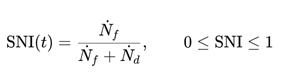 |
(105) |
SNI therefore measures structural generativity rather than structural abundance. SNI > 1/2 corresponds to formation-dominated evolution, SNI = 1/2 to equality between formation and extinction rates, and SNI < 1/2 to an extinction-dominated or structurally infertile regime. In this sense, SNI is a population-level index of cosmic structural natality and is conceptually distinct from the Almeida Growth Index γ_A.
The DUT Fossil Method, developed by the author as a complementary chronometric construction and applied in 2025 to fossil-galaxy dating [71], approaches cosmic chronology from the opposite direction. Rather than measuring the population-level capacity to generate new structures, it treats evolved fossil systems as local gravitational–thermodynamic records of cosmic history. Its characteristic estimator combines the stellar-population stability time t_stable, the elapsed time since peak star formation T_peak, and the gravitational correction t_grav:
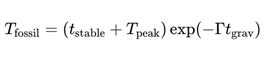 |
(106) |
The three quantities therefore occupy distinct sectors of the DUT framework: γ_A characterizes the growth-sector prediction developed in the present study; SNI quantifies the remaining structural reproductive capacity of the cosmic environment; and the DUT Fossil Method extracts object-level chronological information from evolved fossil structures. Their coexistence records a broader methodological program in which growth, structural natality, and fossil chronology are treated as separate observables rather than as interchangeable measures.
Retraction as Irreversible Structural Exhaustion
In the Dead Universe Theory, retraction is not identified with metric contraction. It does not require the scale factor to reverse, spacetime to contract toward a new singular state, or the Universe to undergo a Big-Crunch-like collapse followed by a renewed Big Bang. This distinguishes the DUT retraction sector from historical oscillatory and modern cyclic/bounce cosmologies in which phases of expansion and contraction are fundamental to the cosmic evolution. Relativistic expansion-contraction models were analyzed by Tolman and Ward [72], while modern cyclic scenarios explicitly connect an expanding epoch to contraction toward a big crunch and a subsequent renewed expanding phase [67,73]. DUT uses the term retraction for a different physical process: the irreversible decline of the capacity of the cosmic medium to generate and sustain organized structure [16,70].
Expansion and retraction are therefore not mutually exclusive in DUT. Large-scale geometry may continue to evolve while structural generativity decreases. In the viscoelastic and entropic interpretation of the framework, retraction is thermodynamic and functional rather than a requirement that cosmological distances globally decrease [1,16]. A convenient asymptotic characterization is
 |
(107) |
where E_use denotes the effective energy remaining available for structural organization and is used here as a phenomenological bookkeeping quantity rather than as an additional fundamental field. The population-level quantity is the Structural Natality Index introduced above, SNI = Ṅ_f/(Ṅ_f+Ṅ_d). Thus the terminal retraction regime is approached as structural birth becomes negligible relative to extinction and fossilization, consistently with the previously defined infertility condition Ṅ_d > Ṅ_f [70].
The endpoint is consequently not a thermodynamic reset. DUT does not require restoration of the cosmos to a special low-entropy initial condition, a compulsory bounce, or a rebirth phase. The thermodynamic arrow remains irreversible,
 |
(108) |
while usable free energy and structural productivity decline. Matter and gravitational fields need not disappear, and the framework does not require all surviving matter to collapse into black holes. Long-lived remnants may instead persist as progressively inactive configurations, including black holes, stellar remnants, quenched galaxies, gravitationally bound dark structures, and other fossilized systems [16,70]. In this sense, structural exhaustion concerns the loss of generative capacity rather than the disappearance of all gravitating content.
This distinction also fixes the meaning of new structure in the late DUT regime. Continued local formation for a finite interval does not constitute a thermodynamic renewal of the Universe. New systems arise from matter, fields, and boundary conditions inherited from prior cosmic evolution and therefore retain what the DUT framework interprets as cosmic structural memory. Successive structures are not thermodynamic replicas of an initial state; they are descendants formed within an increasingly dissipated gravitational-thermodynamic environment. The asymmetry can therefore be summarized as
expansion ≠ unlimited structural growth,
retraction ≠ metric contraction,
cosmic death ≠ cosmic rebirth.
The Dead Universe is therefore not defined as a Universe that geometrically collapses back to its beginning. It is a regime in which gravity and residual structure may persist while the thermodynamic capacity to generate new complexity asymptotically disappears. In this restricted sense, DUT replaces a collapse-and-renewal interpretation with an asymmetric sequence of formation, inheritance, exhaustion, fossilization, and structural death.
In DUT, cosmic death is not a return to the initial state. Gravitational collapse, even when locally extreme, does not imply thermodynamic rejuvenation: a→0 would not, by itself, imply S→0. The theory therefore requires neither a cosmological entropy reset nor a rebirth mechanism. Its terminal state retains the thermodynamic memory of its previous evolution, preserving the irreversible imprint of the preceding cosmic history.
DUT, Cyclic Cosmologies, and the Status of Alternatives to the Big Bang
DUT is not an extension of the Big Bang nor a patch on the standard model. It is a reformulation of the cosmogenic question that avoids the singularity, creation ex nihilo, and pre-existing time without invoking branes, infinite multiverses, or unobservable domains.
Cyclic and bounce cosmologies share with DUT the goal of avoiding the singularity, but do so through different mechanisms — collapse and rebound, in their case [67]; a non-dynamical physical substrate, in the case of DUT. DUT does not claim superiority over these approaches. It claims only to follow a distinct route, with an exact fixed-point structure and a falsifiable prediction within the observable domain: γ_A≈0.618034.
The judgment between routes belongs to the data.
17. Conclusion
A unified microscopic-to-effective framework for the Almeida Growth Index has been developed within the Dead Universe Theory. The scalar–curvature action defines the microscopic gravitational sector, the exact compactification z=ξS2 → O=z/(1+z) provides a bounded order coordinate, center-manifold analysis identifies the slow-mode setting, and the retarded-response/projection construction supplies the causal dimensionality and memory structure required for the subsequent coarse-grained description. The accompanying quasi-stationary test independently excludes the simplest background algebraic route, sharpening the motivation for the causal-history construction.
The key result arises at the causal coarse-graining level. A minimal two-channel unit-multiplicity history transfer law Nn=Nn−1+Nn−2 induces the autonomous ratio map Rn+1=1/(1+Rn). Its unique positive stable fixed point is R*=(√5−1)/2. The fixed-point identity 1−R*=R*2 reproduces D/O=O, and the exact compactification maps the same point to z_c=(1+√5)/2. Identification of the asymptotic ordered fraction with the DUT growth exponent yields γ_A≈0.618034 without observational fitting.
The conjugate-pole structure of the underdamped response is consistent with the two-mode architecture, while the causal-history representation fixes the unit multiplicities independently at the level of the projected history space. From p=q=1, the recurrence, ratio map, unique stable fixed point, constitutive identity, critical coupling, and Almeida Growth Index follow exactly. The resulting γ_A=0.618034 is therefore obtained before observational comparison and without continuous parameter fitting.
Taken together, these results establish a unified causal, thermodynamic, and observational structure for the DUT growth sector. The exact compactification, minimal response realization, projected memory kernel, causal-history recurrence, stable fixed point, integer-multiplicity uniqueness, and the fixed prediction γ_A=0.618034 form a single analytical chain whose numerical value is obtained before observational comparison. The resulting prediction provides a direct point of confrontation with Euclid, DESI, and CSST, while the broader discussion connects this growth-sector result to the DUT substrate, decoherence boundary, structural natality, fossil chronometry, and irreversible retraction framework. The unified construction brings together results that were previously separated across the DUT framework. A natural next step is the direct construction of the projected causal-history quotient from the full scalar–curvature dynamics (Sec. 15.1).
Data availability
No new observational dataset was generated. All results presented here are analytical.
Funding
No external funding is declared for this theoretical study.
Author contributions
Conceptualization, formal analysis, methodology, and writing: Joel Almeida.
Conflicts of interest
The author declares no conflict of interest.
References
- Almeida, J. The Physical Foundations of the Viscoelastic Continuum (DUT): Quantum Decoherence as the Origin of the Dead Substrate. Preprints.org 2026. [Google Scholar] [CrossRef]
- Page, D.N.; Wootters, W.K. Evolution without Evolution: Dynamics Described by Stationary Observables. Phys. Rev. D. 1983, 27, 2885–2892. [Google Scholar] [CrossRef]
- Rovelli, C. Quantum Gravity; Cambridge University Press: Cambridge, 2004. [Google Scholar]
- Brans, C.; Dicke, R.H. Mach’s Principle and a Relativistic Theory of Gravitation. Phys. Rev. 1961, 124, 925–935. [Google Scholar] [CrossRef]
- Bergmann, P.G. Comments on the Scalar-Tensor Theory. Int. J. Theor. Phys. 1968, 1, 25–36. [Google Scholar] [CrossRef]
- Wagoner, R.V. Scalar-Tensor Theory and Gravitational Waves. Phys. Rev. D. 1970, 1, 3209–3216. [Google Scholar] [CrossRef]
- Fujii, Y.; Maeda, K. The Scalar-Tensor Theory of Gravitation; Cambridge University Press: Cambridge, 2003. [Google Scholar]
- Faraoni, V. Cosmology in Scalar-Tensor Gravity; Kluwer Academic Publishers: Dordrecht, 2004. [Google Scholar]
- Sotiriou, T.P.; Faraoni, V. f(R) Theories of Gravity. Rev. Mod. Phys. 2010, 82, 451–497. [Google Scholar]
- De Felice, A.; Tsujikawa, S. f(R) Theories. Living Rev. Relativ. 2010, 13 3. [Google Scholar] [CrossRef] [PubMed]
- Copeland, E.J.; Liddle, A.R.; Wands, D. Exponential Potentials and Cosmological Scaling Solutions. Phys. Rev. D. 1998, 57, 4686–4690. [Google Scholar] [CrossRef]
- Copeland, E.J.; Sami, M.; Tsujikawa, S. Dynamics of Dark Energy. Int. J. Mod. Phys. D. 2006, 15, 1753–1936. [Google Scholar] [CrossRef]
- Bahamonde, S.; Böhmer, C.G.; Carloni, S.; Copeland, E.J.; Fang, W.; Tamanini, N. Dynamical Systems Applied to Cosmology: Dark Energy and Modified Gravity. Phys. Rep. 2018, 775–777, 1–122. [Google Scholar] [CrossRef]
- Wainwright, J.; Ellis, G.F.R. (Eds.) Dynamical Systems in Cosmology; Cambridge University Press: Cambridge, 1997. [Google Scholar]
- Almeida, J. Effective Ξμν Closure and the Almeida Growth Index: γ_A = 0.618 as a Distinct Alternative to the ΛCDM Growth Index (γ ≈ 0.55). Parent effective DUT formulation/manuscript. MDPI 2026. [Google Scholar]
- Almeida, J. Dead Universe Theory: field formalism, entropic retraction, autonomous fossilisation dynamics, and scalar–curvature coupling. Preprints.org 2025. [Google Scholar] [CrossRef]
- Nakajima, S. On Quantum Theory of Transport Phenomena: Steady Diffusion. Prog. Theor. Phys. 1958, 20, 948–959. [Google Scholar]
- Mori, H. Transport, Collective Motion, and Brownian Motion. Prog. Theor. Phys. 1965, 33, 423–455. [Google Scholar] [CrossRef]
- Zwanzig, R. Memory Effects in Irreversible Thermodynamics. Phys. Rev. 1961, 124, 983–992. [Google Scholar] [CrossRef]
- Kubo, R. The Fluctuation-Dissipation Theorem. Rep. Prog. Phys. 1966, 29, 255–284. [Google Scholar] [CrossRef]
- Zwanzig, R. Nonequilibrium Statistical Mechanics; Oxford University Press: Oxford, 2001. [Google Scholar]
- Feynman, R.P.; Vernon, F.L. The Theory of a General Quantum System Interacting with a Linear Dissipative System. Ann. Phys. 1963, 24, 118–173. [Google Scholar] [CrossRef]
- Caldeira, A.O.; Leggett, A.J. Path Integral Approach to Quantum Brownian Motion. Physica A 1983, 121, 587–616. [Google Scholar] [CrossRef]
- Breuer, H.-P.; Petruccione, F. The Theory of Open Quantum Systems; Oxford University Press: Oxford, 2002. [Google Scholar]
- Weiss, U. Quantum Dissipative Systems, 4th ed.; World Scientific: Singapore, 2012. [Google Scholar]
- Wilson, K.G.; Kogut, J. The Renormalization Group and the ε Expansion. Phys. Rep. 1974, 12, 75–199. [Google Scholar] [CrossRef]
- Kadanoff, L.P. Scaling Laws for Ising Models Near T_c. Physics 1966, 2, 263–272. [Google Scholar] [CrossRef]
- Fisher, M.E. The Renormalization Group in the Theory of Critical Behavior. Rev. Mod. Phys. 1974, 46, 597–616. [Google Scholar] [CrossRef]
- Hohenberg, P.C.; Halperin, B.I. Theory of Dynamic Critical Phenomena. Rev. Mod. Phys. 1977, 49, 435–479. [Google Scholar] [CrossRef]
- Cardy, J. Scaling and Renormalization in Statistical Physics; Cambridge University Press: Cambridge, 1996. [Google Scholar]
- Goldenfeld, N. Lectures on Phase Transitions and the Renormalization Group; Addison-Wesley: Reading, 1992. [Google Scholar]
- Stanley, H.E. Introduction to Phase Transitions and Critical Phenomena; Oxford University Press: Oxford, 1971. [Google Scholar]
- Birrell, N.D.; Davies, P.C.W. Quantum Fields in Curved Space; Cambridge University Press: Cambridge, 1982. [Google Scholar]
- Parker, L.; Toms, D. Quantum Field Theory in Curved Spacetime; Cambridge University Press: Cambridge, 2009. [Google Scholar]
- Buchbinder, I.L.; Odintsov, S.D.; Shapiro, I.L. Effective Action in Quantum Gravity; IOP Publishing: Bristol, 1992. [Google Scholar]
- Parker, L.; Fulling, S.A. Adiabatic Regularization of the Energy-Momentum Tensor of a Quantized Field in Homogeneous Spaces. Phys. Rev. D. 1974, 9, 341–354. [Google Scholar] [CrossRef]
- Peebles, P.J.E. The Large-Scale Structure of the Universe; Princeton University Press: Princeton, 1980. [Google Scholar]
- Linder, E.V. Cosmic Growth History and Expansion History. Phys. Rev. D. 2005, 72, 043529. [Google Scholar] [CrossRef]
- Wang, L.; Steinhardt, P.J. Cluster Abundance Constraints on Quintessence Models. Astrophys. J. 1998, 508, 483–490. [Google Scholar] [CrossRef]
- Huterer, D.; Linder, E.V. Separating Dark Physics from Physical Darkness: Minimalist Modified Gravity versus Dark Energy. Phys. Rev. D. 2007, 75, 023519. [Google Scholar] [CrossRef]
- Joyce, A.; Jain, B.; Khoury, J.; Trodden, M. Beyond the Cosmological Standard Model. Phys. Rep. 2015, 568, 1–98. [Google Scholar] [CrossRef]
- Carr, J. Applications of Centre Manifold Theory; Springer-Verlag: New York, 1981. [Google Scholar]
- Guckenheimer, J.; Holmes, P. Nonlinear Oscillations, Dynamical Systems, and Bifurcations of Vector Fields; Springer: New York, 1983. [Google Scholar]
- Wiggins, S. Introduction to Applied Nonlinear Dynamical Systems and Chaos, 2nd ed.; Springer: New York, 2003. [Google Scholar]
- Perko, L. Differential Equations and Dynamical Systems, 3rd ed.; Springer: New York, 2001. [Google Scholar]
- Zurek, W.H. Decoherence, Einselection, and the Quantum Origins of the Classical. Rev. Mod. Phys. 2003, 75, 715–775. [Google Scholar] [CrossRef]
- Schlosshauer, M. Decoherence and the Quantum-to-Classical Transition; Springer: Berlin, 2007. [Google Scholar]
- Hu, B.L.; Paz, J.P.; Zhang, Y. Quantum Brownian Motion in a General Environment: Exact Master Equation with Nonlocal Dissipation and Colored Noise. Phys. Rev. D. 1992, 45, 2843–2861. [Google Scholar] [CrossRef] [PubMed]
- Leggett, A.J.; Chakravarty, S.; Dorsey, A.T.; Fisher, M.P.A.; Garg, A.; Zwerger, W. Dynamics of the Dissipative Two-State System. Rev. Mod. Phys. 1987, 59, 1–85. [Google Scholar] [CrossRef]
- Izvekov, S. Mori-Zwanzig Projection Operator Formalism: Particle-Based Coarse-Grained Dynamics of Open Classical Systems Far from Equilibrium. Phys. Rev. E 2021, 104, 024121. [Google Scholar] [CrossRef] [PubMed]
- Widder, C.; Zimmer, J.; Schilling, T. On the Generalized Langevin Equation and the Mori Projection Operator Technique. J. Phys. A Math. Theor. 2025, 58, 405001. [Google Scholar] [CrossRef]
- Amendola, L.; Kunz, M.; Sapone, D. Measuring the Dark Side (with Weak Lensing). J. Cosmol. Astropart. Phys. 2008, 04, 013. [Google Scholar] [CrossRef]
- Guzzo, L.; et al. A Test of the Nature of Cosmic Acceleration Using Galaxy Redshift Distortions. Nature 2008, 451, 541–544. [Google Scholar] [CrossRef] [PubMed]
- Percival, W.J.; White, M. Testing Cosmological Structure Formation Using Redshift-Space Distortions. Mon. Not. R. Astron. Soc. 2009, 393, 297–308. [Google Scholar] [CrossRef]
- Landau, L.D.; Lifshitz, E.M. Statistical Physics, Part 1, 3rd ed.; Pergamon Press: Oxford, 1980. [Google Scholar]
- Onsager, L. Reciprocal Relations in Irreversible Processes. I. Phys. Rev. 1931, 37, 405–426. [Google Scholar] [CrossRef]
- Prigogine, I. Introduction to Thermodynamics of Irreversible Processes, 3rd ed.; Wiley-Interscience: New York, 1967. [Google Scholar]
- Starobinsky, A.A. Stochastic De Sitter (Inflationary) Stage in the Early Universe. In Field Theory, Quantum Gravity and Strings; Springer: Berlin, 1986; pp. 107–126. [Google Scholar]
- Hu, B.L.; Verdaguer, E. Stochastic Gravity: Theory and Applications. Living Rev. Relativ. 2008, 11 3. [Google Scholar] [CrossRef]
- Euclid Collaboration; Mellier, Y.; et al. Euclid - I. Overview of the Euclid mission. Astron. Astrophys. 2025, 697, A1. [Google Scholar] [CrossRef]
- DESI Collaboration. DESI Surpasses Original Five-Year Survey Goals. DESI 2026. [Google Scholar]
- Miao, H.; Gong, Y.; Li, X.-D.; Zhan, H.; et al. Cosmological constraint precision of photometric and spectroscopic multi-probe surveys of China Space Station Telescope (CSST). Mon. Not. R. Astron. Soc. 2023, 519, 1132–1148. [Google Scholar] [CrossRef]
- Hawking, S.W.; Penrose, R. The Singularities of Gravitational Collapse and Cosmology. Proc. R. Soc. A 1970, 314, 529–548. [Google Scholar] [CrossRef]
- Guth, A.H. Inflationary Universe: A Possible Solution to the Horizon and Flatness Problems. Phys. Rev. D. 1981, 23, 347–356. [Google Scholar] [CrossRef]
- Rovelli, C. Loop Quantum Gravity. Living Rev. Relativ. 2008, 11 5. [Google Scholar] [CrossRef] [PubMed]
- Randall, L.; Sundrum, R. Large Mass Hierarchy from a Small Extra Dimension. Phys. Rev. Lett. 1999, 83, 3370–3373. [Google Scholar] [CrossRef]
- Steinhardt, P.J.; Turok, N. Cosmic Evolution in a Cyclic Universe. Phys. Rev. D. 2002, 65, 126003. [Google Scholar] [CrossRef]
- Newton, I. Philosophiae Naturalis Principia Mathematica, 2nd ed.; General Scholium: Cambridge, 1713. [Google Scholar]
- Almeida, J. The “Dead Universe” Theory: Natural Separation of Galaxies Driven by the Remnants of a Supermassive Dead Universe. Nat. Sci. 2024, 16, 65–101. [Google Scholar] [CrossRef]
- Almeida, J. The Dead Universe Theory (DUT): The Asymmetric Thermodynamic Retraction of the Universe and the Foundations of Cosmic Infertility. Open Access Libr. J. 2025, 12, 1–35. [Google Scholar] [CrossRef]
- Almeida, J. The Universe is 76.8 Billion Years Old: Dating by the Fossil Method Applied to the Galaxy KiDS J0842+0059 via DUT Quantum Simulator. Zenodo 2025. [Google Scholar] [CrossRef]
- Tolman, R.C.; Ward, M. On the Behavior of Non-Static Models of the Universe When the Cosmological Term Is Omitted. Phys. Rev. 1932, 39, 835–843. [Google Scholar] [CrossRef]
- Khoury, J.; Ovrut, B.A.; Seiberg, N.; Steinhardt, P.J.; Turok, N. From Big Crunch to Big Bang. Phys. Rev. D. 2002, 65, 086007. [Google Scholar] [CrossRef]

Table 1.
Structural selectivity of the causal-history architecture. The present follow-up recovers the effective-sector value established in Almeida [15]. Within the two-channel integer-multiplicity family, Sec. 8.6.6 proves that compatibility with this value uniquely selects (p,q)=(1,1). The alternatives shown here generate distinct fixed points, providing a direct numerical illustration of the algebraic selectivity of the result.
Table 1.
Structural selectivity of the causal-history architecture. The present follow-up recovers the effective-sector value established in Almeida [15]. Within the two-channel integer-multiplicity family, Sec. 8.6.6 proves that compatibility with this value uniquely selects (p,q)=(1,1). The alternatives shown here generate distinct fixed points, providing a direct numerical illustration of the algebraic selectivity of the result.
| Structure | Characteristic equation | R* | Status |
|---|---|---|---|
| 2 channels, unit weight (adopted) | R2+R−1=0 | 0.618034 | Adopted architecture |
| 2 channels, p=1, q=2 | 2R2+R−1=0 | 0.500000 | Alternative |
| 2 channels, p=2, q=1 | R2+2R−1=0 | 0.414214 | Alternative |
| 3 channels, unit weight | R3+R2+R−1=0 | 0.543689 | Alternative |
| 4 channels, unit weight | R4+R3+R2+R−1=0 | 0.518790 | Alternative |
Disclaimer/Publisher’s Note: The statements, opinions and data contained in all publications are solely those of the individual author(s) and contributor(s) and not of MDPI and/or the editor(s). MDPI and/or the editor(s) disclaim responsibility for any injury to people or property resulting from any ideas, methods, instructions or products referred to in the content. |
© 2026 by the authors. Licensee MDPI, Basel, Switzerland. This article is an open access article distributed under the terms and conditions of the Creative Commons Attribution (CC BY) license (http://creativecommons.org/licenses/by/4.0/).
Copyright: This open access article is published under a Creative Commons CC BY 4.0 license, which permit the free download, distribution, and reuse, provided that the author and preprint are cited in any reuse.