

Submitted:
22 September 2026
Posted:
24 September 2026
You are already at the latest version
Abstract
This study aims to reduce biases in diffuse irradiance modelling at sub-hourly time scales, which is critical for accurate photovoltaic system performance simulations. Typically, this process involves estimating diffuse horizontal irradiance (DHI) from global horizontal irradiance (GHI) and then applying a decomposition model to determine the irradiance on the PV module plane. While models like Erbs and Perez are standard, they introduce biases when applied to shorter time scales (e.g., 1-minute) without adaptation. Leveraging global ground-based datasets, this work compares common DHI and decomposition models and reparametrizes their coefficients specifically for subhourly scales. The results demonstrate that these improvements reduce mean bias in yearly simulation estimates. We also discuss requirements for further improvements.
Keywords:
solar
; photovoltaic
; irradiance
; diffuse irradiance
; model
; simulation
1. Introduction
Evaluating the different solar irradiance components precisely is critical for accurate photovoltaic system performance simulations. Furthermore, sub-hourly simulations are becoming ubiquitous due to their ability to better represent the dynamic of real PV systems. This requires the precise evaluation of sub-hourly time series of the different irradiance components.
However, measurements of all the different solar irradiance components are not always available, in particular for the early design stage of a new power plant, and it is common to have to rely only on Global Horizontal Irradiance (GHI) time series as input. Finer components are then usually evaluated using two modelling stages.
First, if no component-specific measurement is available, GHI is decomposed into Diffuse Horizontal Irradiance (DHI) and Direct Normal Irradiance (DNI) using a function describing the correlation between GHI and the diffuse fraction. Then, the diffuse irradiance may be further decomposed into components representing contributions from different parts of the sky. These are then, together with the contribution from the ground albedo, geometrically transposed and combined into an irradiance incident to the plane of array (POA). Figure 1 synthetically represents these modelling steps and variables.
Erbs [1] and Perez [2] models are commonly used to perform those two steps, the diffuse and transposition model, respectively. However, they were developed using mostly hourly data and applying them without adaptation to finer time scales introduces biases. Moreover, extensive worldwide ground-based radiation measurement datasets are now available [4], enabling a more universal reparameterization of irradiance models.
This work aims at characterizing the bias introduced by these models at sub-hourly timescales and proposes adapted coefficients to minimize biases at all timescales. These coefficients, as implemented in PVsyst 8.1.6, are then used to estimate the remaining associated uncertainty, in yearly yield estimates in two typical mount-type simulation scenarios.
2. Dataset and Filtering
To evaluate the model performances and refit their coefficients on a representative dataset, we use the IEA-PVPS ground-measured irradiance dataset [4]. It consists of 1-minute records of GHI, DHI, and DNI data measured at 113 sites around the world.
These data undergo two steps of filtering. First, a series of filters are applied on the 1-minute data, following the current recommended best practice [5]. From this reference, we apply
- the physically possible limits tests,
- the extremely rare limits tests,
- the closure equation tests,
- the k-index tests,
- the DNI tracker test,
- and, additionally, we filter out data points with zenith angle below 85°, as these data points suffer from strong uncertainties while contributing negligibly to the PV production.
Note that the DNI data are not used further in the present work and are only used to check the consistency between the three measured irradiances.
Second, the data are aggregated to coarser timestep durations, specifically 2, 3, 4, 5, 6, 10, 12, 15, 20, 30, and 60 minutes, by taking their averages over these respective intervals. Prior to this, to ensure the data are comparable at each timestep duration, we filtered further the 1-minute data by keeping only the 60-minute slices that have zero flagged records. Hereafter, we name this step “Perfect Hours” filtering.
Figure 2.
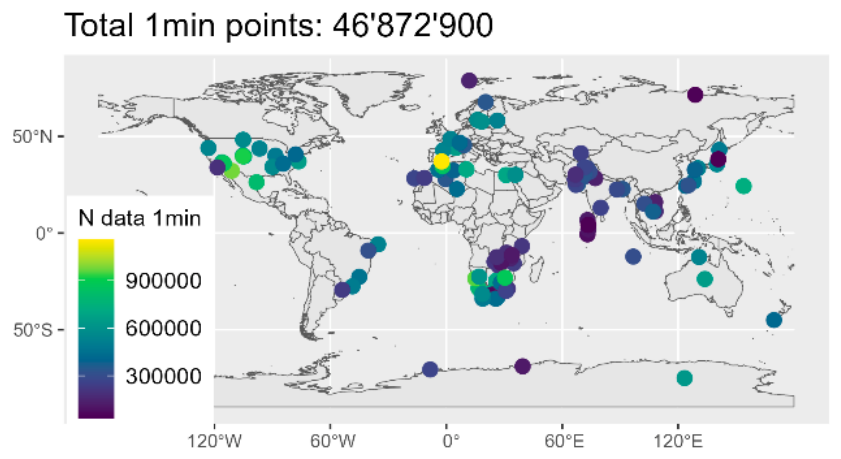
Location of the 113 stations of the IEA-PVPS radiation dataset [4] and number of 1 minute data points remaining after filtering.
Figure 2.
Location of the 113 stations of the IEA-PVPS radiation dataset [4] and number of 1 minute data points remaining after filtering.
3. Diffuse Irradiance Models: From GHI to DHI
When diffuse irradiation is not directly measured, it must be estimated from global horizontal or POA irradiances using a model. This is, for example, the case for satellite weather data, for which the diffuse component is modelled based on the input GHI time series. This is also the case for ground-based measurements when a single pyranometer is used.
A wide variety of models exist in the literature, with several candidates having similar accuracy [6] [7]. However, an important further requirement in the context of industry-level PV system simulations is that it relies on inputs that are generally available to the practitioner. The following models all use GHI as well as longitude, latitude, and time stamps to compute the solar geometry.
The Erbs model [1] is a simple yet effective correlation function of the diffuse fraction vs. the clearness index , given by the piecewise equation
with , , and where EHI is the extraterrestrial irradiance projected on the horizontal plane. This equation was originally fitted using hourly ground-measured irradiance data from four U.S. locations [1] and has a reasonable precision for hourly simulations. However, its precision is known to degrade for sub-hourly timescales [8]. For example, it cannot represent well the fast dynamics of cloud irradiance enhancement, for which values above 1 can be measured due to momentary increases in diffuse irradiance [9].
The ENGERER2 model [10] (E2) uses the same original inputs as the Erbs model, i.e. GHI, longitude, latitude, and time stamps, to estimate DHI. To improve its prediction, it relies on additional intermediate indicators of the weather conditions, which are
- –
- , which is the clearness index for the clear-sky global horizontal irradiance ,
- –
- , representing the variation between the two clearness indices,
- –
- , intending to capture cloud-enhancement features,
- –
- , the apparent solar time,
- –
- , the solar zenith angle.
Similarly to the Erbs model, the E2 model relates the diffuse fraction to those predictors, using a logistic equation form
where and are fitting coefficients.
Since the last publication of the model [10], larger datasets of 1-minute ground-measured global and diffuse irradiances have been made available. Our implementation proposes a new fit of the E2 coefficients based on the above dataset, aggregated at timestep durations of 1, 2, 3, 4, 5, 6, 10, 12, 15, 20, 30, and 60 minutes. It is realised by minimizing the Root Mean Squared Error (RMSE) over all measurements ,
using, as in [10], the Nelder–Mead non-linear minimisation algorithm.
Figure 3 illustrates the performance of both models over the whole dataset. For a comparison closer to the typical scope of PV system yield simulations, the data are regrouped by site and year, and for each site-year, we compute the mean measured value (M), the normalized Mean Bias Error (nMBE), and normalized RMSE (nRMSE),
The main improvement brought by the E2 model and our refit of its coefficients is visible in the median nMBE, which is very close to zero for all time step durations. A small residual bias is visible at dt=20 min, which we attribute to a non-perfect convergence of the non-linear least square fitting. In comparison, the Erbs model performs worse, with a systematic increase of the median nMBE as the time step duration is reduced, reaching almost 5% at dt=1min. Nonetheless, this improvement over the median is contrasted by the very large interdecile range, where lie 80% of the site-years of the dataset. This means that randomly selecting one site and one year, the diffuse model can lead to errors on the yearly diffuse irradiance between approximatively -15% to +20%. Fortunately, since this is a decomposition model, this error is balanced by an error of the opposite magnitude on the direct component (not shown), and we will see in section 5 that it has a smaller impact on the yield estimation of typical PV power plant.
Figure 4 shows the emblematic correlation vs. , which helps understand the models’ weaknesses and discuss paths for improvement. While the E2 model flexibility allows a partial description of cloud enhancement (values with high for ), both models fail to properly explore the regions where the data points are most concentrated (around for and around ). They also fail to explore the large horizontal spread of the distribution. Given the small amount of fitting parameters of the E2 model compared to the size of the dataset, its parametrization could be easily extended to account either for additional predictors or for cross-correlations among the ones already used. This would introduce additional fitting parameters, allowing these to stretch further the logistic equation of the model, while keeping low the risk of over-fitting. The latter could be then diagnosed by splitting the dataset between training and testing sets.
Other avenues of improvement have been explored in the literature. YANG5 developed climatologic regime-dependent coefficients using satellite measurements such as aerosol optical depth, albedo, and a so-called cloud-day frequency [11]. A second notable example is the GISPLIT model which draws further correlation from the variability of the GHI time series, sorting each time step in classes of variability, each of which leads to a different diffuse model parametrization [12]. These approaches were shown to further reduce the median nRMSE to around 30%, lower than the ~40% reached by the most common models [12] such as Erbs, E2, DIRINT [13] or DIRINDEX [14]. Nevertheless, they suffer from a smaller application scope: they were developed only for time durations of 1-minute, and their regime-based coefficients make them non-bijective, which prevents their use for retro-transposition in case only the POA irradiance is available.
4. Transposition to Plane of Array: From (GHI;DHI) to Diffuse Components
Once both GHI and DHI are known, the next modelling step transposes horizontal irradiances to the plane of array in two successive sub steps: Decomposing the sky-diffuse irradiance contribution into several subcomponents, which are then mapped into the plane of array by simple geometrical transformations. Widely used models such the Hay-Davies [15] and the Perez [2] models, which are implemented by PVsyst, function in this way. Figure 1 illustrates this by highlighting the circumsolar contribution, common to the Hay-Davis and Perez models, while their mathematical description and more details on their implementation can be found in our previous work [3]. In this previous work, we already highlighted the problematic that the 48 fitting coefficients used in the diffuse irradiance decomposition of the Perez model were obtained using a mostly hourly dataset.
Ideally a large dataset of 1-minute worldwide POA irradiance data should be used to refit Perez’s transposition model coefficients and evaluate the absolute performance of the model, but such a dataset is unfortunately not available to us at present. However, considering the hourly Perez coefficients as reference, we can refit the coefficients of the model at sub-hourly timescales so that their predictions, once aggregated at the hour, matches with the reference. This is illustrated in Figure 5. Minimizing the discrepancy is done using a traditional linear least square fitting on the horizontal and vertical components (see [3] for details), which has the mathematical property to lead to zero bias on those.
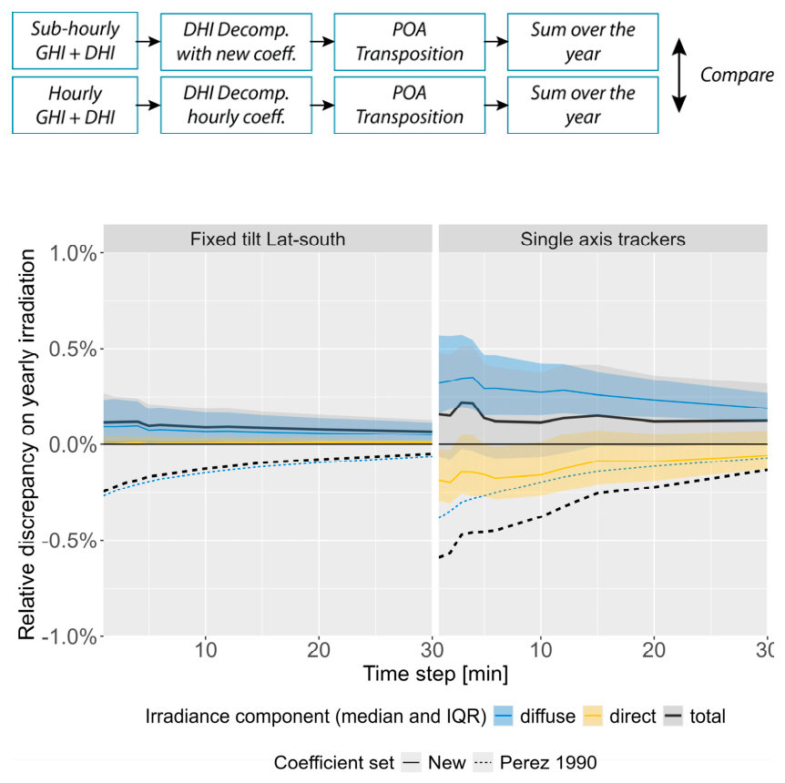
However, a bias can still form once the components are transposed into the POA. In Figure 6, we show how the yearly POA irradiation compares between using the hourly reference or the new coefficients for each sub-hourly timestep durations. We compare the results for two mount types, simulated at each site-year of the dataset: a fixed tilt installation south-oriented, where the tilt is adapted to the
latitude, and a single axis tracker, with the axis oriented along the north-south line. For both system types, the increasing median bias at finer timescales introduced by the reference model is successfully mitigated using the new set of coefficients, below 0.1-0.2%. In the case of the fixed tilt system, the remaining bias is dominated by the diffuse component in the POA, while in the case of trackers, diffuse and direct components compensate. The inter quartile range is larger for the tracker case, but even in that case the bias is smaller than 0.5%. Keep in mind that theses comparisons are made relative to the hourly Perez model and are not a qualification of the error made against real measured POA irradiances.
5. Impacts on Solar Resource for Typical Power Plants
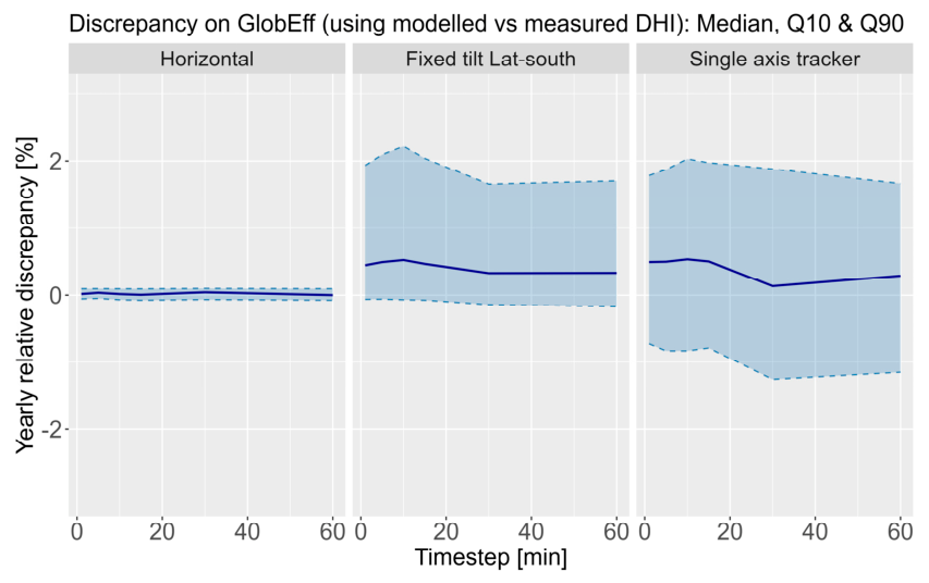
In this section, we explore the impact of using our reparametrized DHI model compared to using DHI measurements as simulation input for PVsyst (version 8.1.6). We take as key performance index the irradiance in the POA, corrected by the Incidence Angle Modifier (IAM) function of the PV module, spectral correction and linear shading loss (PVsyst variable ‘GlobEff’). As in the previous section, the comparison is carried at each site-year of the dataset, for three mount types: a fixed tilt and single-axis tracker installation as in the previous section, as well as for a horizontal installation for reference.
As expected, the error for the horizontal system is almost zero, since GHI is also a simulation input. The residual spread is due to the IAM correction which is applied on each component depending on their incidence angle, or the integral thereof in case of a distributed contribution. Note that the spectral correction model in PVsyst v8.1.6 applies the same correction to diffuse and direct component. A refined model considering them separately would lead to an additional spread.
Moving to the fixed tilt and single-axis tracker systems, a small residual median bias of about 0.5% is present. This bias is consistent with the DHI model residual bias. The distribution over site-years is more asymmetric for fixed tilt (~0 to 2%) than for trackers (-1 to 2%).
The impact of “Perfect hours” filtering might have lowered slightly the importance of shading in this study, since it systematically cuts hours in the morning and evening. Indeed, predicting a wrong diffuse fraction influences the magnitude of the electrical shading loss. This impact, that we expect to be very small on yearly irradiation, will be studied in future work.
The case where only POA measurements data are available, requiring the use of the diffuse irradiance model in combination with a transposition model to reconstruct GHI and DHI, will also be discussed in future work.
Figure 7.
Yearly relative discrepancy in the plane-of-array irradiance, corrected by IAM, spectral correction and linear shading (GlobEff), between simulations using the measured vs modelled DHI. The statistics over all site-years is represented by the percentiles P10, P90 (dashed lines) and median P50 (solid lines).
Figure 7.
Yearly relative discrepancy in the plane-of-array irradiance, corrected by IAM, spectral correction and linear shading (GlobEff), between simulations using the measured vs modelled DHI. The statistics over all site-years is represented by the percentiles P10, P90 (dashed lines) and median P50 (solid lines).
6. Conclusion
Reparametrizing the diffuse irradiance and transposition models successfully maintains a consistent mean bias across all sub-hourly timescales, lowered compared to reference in both cases. Comparing the diffuse modelling against measurements from numerous sites reveals a median impact of approximately 0.5% in yearly POA irradiation, with a spread between -1% and +2%. Performance could be further enhanced by improving fitting convergence and utilizing models with additional parameters. Regarding the transposition model, our reparameterization eliminates the artificial bias caused by the unmodified use of Perez’s 1990 coefficients, keeping the bias below 0.25% for typical systems. Nevertheless, a comprehensive dataset of 1-minute plane-of-array data is required to fully characterize modelling errors at short time scales. Both models with their sub-hourly dedicated coefficients are implemented in PVsyst version 8.1. The coefficients values of the diffuse decomposition model and the transposition model may be made available upon contact with PVsyst.
Conflicts of Interest
The authors all work for PVsyst SA.
References
- Erbs, D. G.; Klein, S. A.; Duffie, J. A. Estimation of the diffuse radiation fraction for hourly, daily and monthly-average global radiation. Sol. Energy 1982, vol. 28, 293–302. [Google Scholar] [CrossRef]
- Perez, R.; Ineichen, P.; Seals, R.; Michalsky, J.; Stewart, R. Modeling daylight availability and irradiance components from direct and global irradiance. Sol. Energy 1990, vol. 44, 271–289. [Google Scholar] [CrossRef]
- Oliosi, M.; Wittmer, B.; Mermoud, A.; Bridel-Bertomeu, A. Accounting for Sub-Hourly Irradiance Fluctuations in Hourly Performance Simulations. 40th European Photovoltaic Solar Energy Conference and Exhibition, 2023. [Google Scholar]
- Forstinger, Y.-M.; Saint-Drenan; Wilbert, S.; Jensen, A.; Kraas, B.; Peruchena, C. F.; Gueymard, C.; Ronzio, D.; Yang, D.; Collino, E.; Martinez, J. P.; Ruiz-Arias, J.; Hanrieder, N.; Blanc, P. IEA-PVPS Task-16 Reference Solar Measurements. 2021. [Google Scholar]
- Forstinger; Wilbert, S.; Kraas, B.; Fernández Peruchena, C.; Gueymard, C. A.; Collino, E.; Ruiz-Arias, J. A.; Polo Martinez, J.; Saint-Drenan, Y.-M.; Ronzio, D.; Hanrieder, N.; Jensen, A. R.; Yang, D. Expert Quality Control of Solar Radiation Ground Data Sets. In Proceedings of the ISES Solar World Congress 2021, Virtual, 2021. [Google Scholar]
- Sengupta, M.; Habte, A.; Wilbert, S.; Gueymard, C.; Remund, J.; Lorenz, E.; Sark, W. v.; Jensen; Adam, R. Best Practices Handbook for the Collection and Use of Solar Resource Data for Solar Energy Applications: Fourth Edition; 2024. [Google Scholar]
- Ruiz-Arias, J. A.; Gueymard, C. A. Solar irradiance component separation benchmarking: The critical role of dynamically-constrained sky conditions. Renew. Sustain. Energy Rev. 2024, vol. 202, 114678. [Google Scholar] [CrossRef]
- R. A. Gansler, K. S.A. and W. A. Beckman. Investigation of minutes solar radiation data. Sol. Energy 1995, vol. 55, 21–27. [CrossRef]
- Emck, P.; Richter, M. An Upper Threshold of Enhanced Global Shortwave Irradiance in the Troposphere Derived from Field Measurements in Tropical Mountains. J. Appl. Meteorol. Climatol. 2008, vol. 47, 2828–2845. [Google Scholar] [CrossRef]
- Bright, J. M.; Engerer, N. A. Engerer2: Global re-parameterisation, update, and validation of an irradiance separation model at different temporal resolutions. J. Renew. Sustain. Energy 2019, vol. 11, 033701. [Google Scholar] [CrossRef]
- Yang, D.; Gu, Y.; Mayer, M. J.; Gueymard, C. A.; Wang, W.; Kleissl, J.; Li, M.; Chu, Y.; Bright, J. M. Regime-dependent 1-min irradiance separation model with climatology clustering. Renew. Sustain. Energy Rev. 2024, vol. 189, 113992. [Google Scholar] [CrossRef]
- Ruiz-Arias, J. A.; Gueymard, C. A. GISPLIT: High-performance global solar irradiance component-separation model dynamically constrained by 1-min sky conditions. Sol. Energy 2024, vol. 269, 112363. [Google Scholar] [CrossRef]
- Perez, R.; Ineichen, P.; Maxwell, E. L.; Seals, R. D.; Zelenka, A. Dynamic global-to-direct irradiance conversion models. ASHRAE Trans. 1992, vol. 98, 354–369. [Google Scholar]
- Perez, R.; Ineichen, P.; Moore, K.; Kmiecik, M.; Chain, C.; George, R.; Vignola, F. A new operational model for satellite-derived irradiances: description and validation. Sol. Energy 2002, vol. 73, 307–317. [Google Scholar] [CrossRef]
- Hay, J. E.; Davies, J. A. Calculations of the solar radiation incident on an inclined surface. Proceedings: First Canadian Solar Radiation Data Workshop, 1980. [Google Scholar]
- Thorning, J. K.; Hass, T. K.; Spataru, S. V. Evaluation of Irradiance Decomposition Models and Their Predictors. 40th European Photovoltaic Solar Energy Conference and Exhibition, 2023; p. 020362–001–020362–011. [Google Scholar]
Figure 1.
Flow diagram of the irradiance decomposition modelling steps. Note that the Perez model includes a contribution from the horizon band HBndVrt, proportional to DHI. DifSInc includes all sky components in plane, excluding circumsolar CircInc and beam BeamInc. Finally, bringing in the albedo contribution Alb_Inc results in the POA irradiance GlobInc. More thorough discussion and details on the implementation in PVsyst can be found in [3].
Figure 1.
Flow diagram of the irradiance decomposition modelling steps. Note that the Perez model includes a contribution from the horizon band HBndVrt, proportional to DHI. DifSInc includes all sky components in plane, excluding circumsolar CircInc and beam BeamInc. Finally, bringing in the albedo contribution Alb_Inc results in the POA irradiance GlobInc. More thorough discussion and details on the implementation in PVsyst can be found in [3].
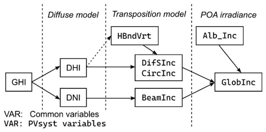
Figure 3.
nMBE and nRMSE at all time step durations of Erbs and Engerer2 model, the latter using our refitted coefficients. The statistics over all site-years is represented by the percentiles P10, P90 (dashed lines) and median P50 (solid lines).
Figure 3.
nMBE and nRMSE at all time step durations of Erbs and Engerer2 model, the latter using our refitted coefficients. The statistics over all site-years is represented by the percentiles P10, P90 (dashed lines) and median P50 (solid lines).
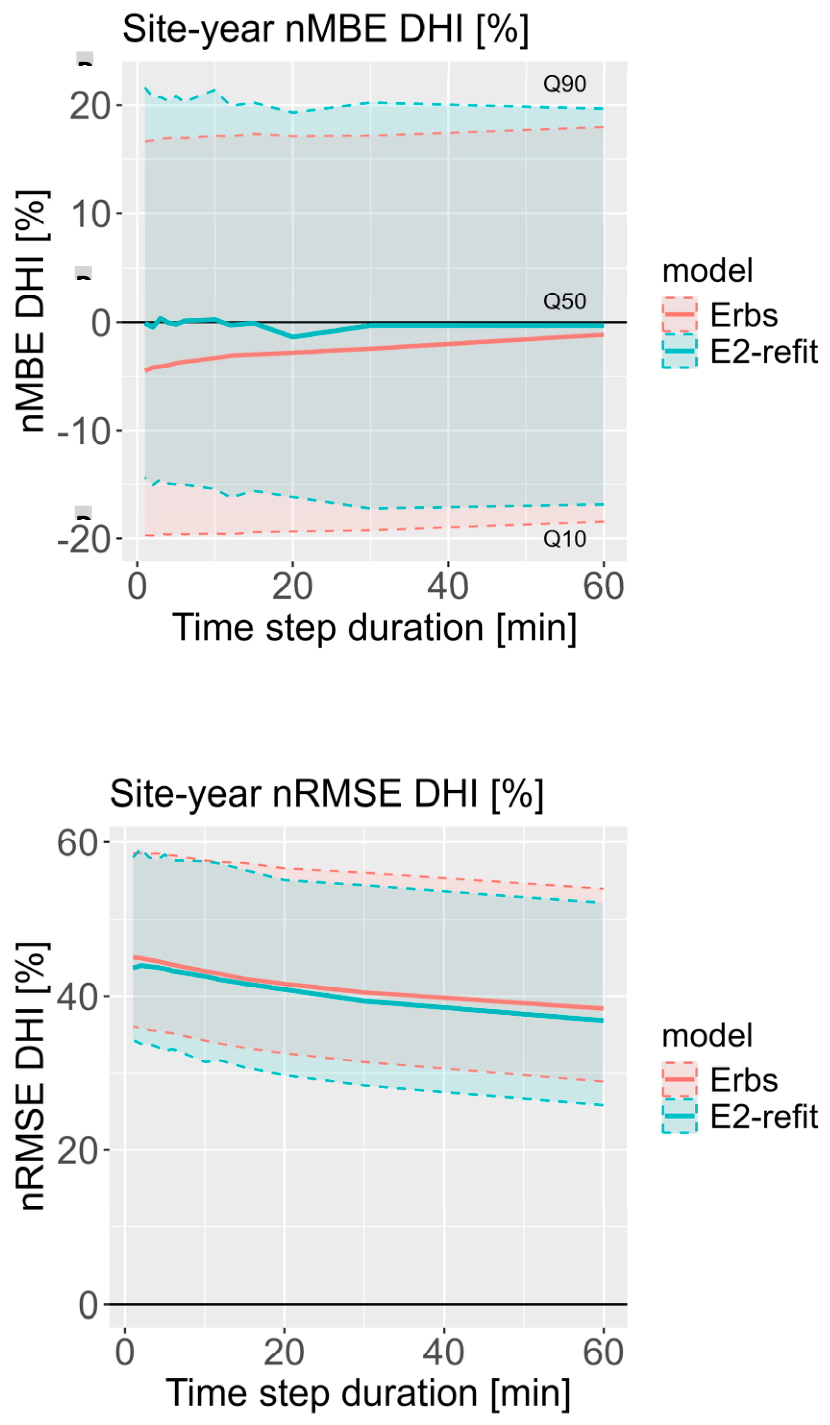
Figure 4.
vs correlation for Erbs and E2 model compared to 1-minute measurements.
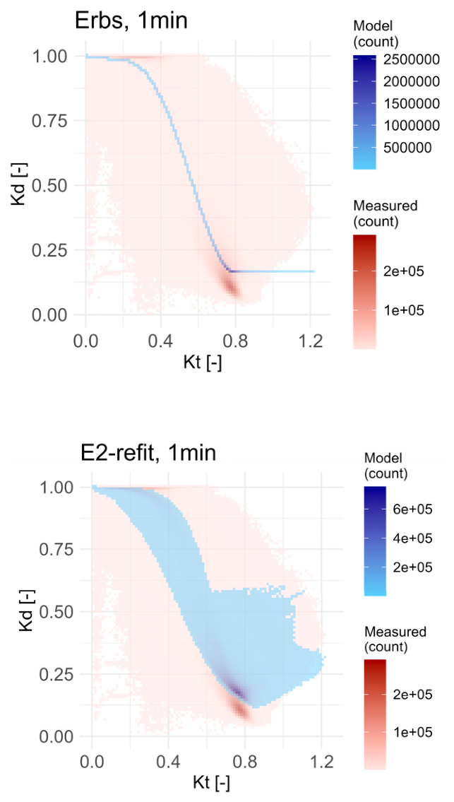
Figure 5.
Methodology to refit the transposition model coefficients at sub-hourly timescales, using the hourly Perez model as reference. This method is used to obtain new coefficients for time step durations of 1, 2, 3, 4, 5, 6, 10, 12, 15, 20 and 30 minutes.
Figure 5.
Methodology to refit the transposition model coefficients at sub-hourly timescales, using the hourly Perez model as reference. This method is used to obtain new coefficients for time step durations of 1, 2, 3, 4, 5, 6, 10, 12, 15, 20 and 30 minutes.
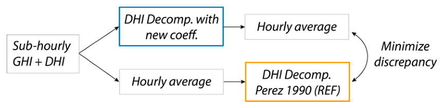
Figure 6.
Discrepancy in yearly POA irradiance (GlobInc in PVsyst terminology), between the reference hourly transposition model and the model using coefficients adapted to sub-hourly time step durations. IQR stands for inter quartile range.
Figure 6.
Discrepancy in yearly POA irradiance (GlobInc in PVsyst terminology), between the reference hourly transposition model and the model using coefficients adapted to sub-hourly time step durations. IQR stands for inter quartile range.
Disclaimer/Publisher’s Note: The statements, opinions and data contained in all publications are solely those of the individual author(s) and contributor(s) and not of MDPI and/or the editor(s). MDPI and/or the editor(s) disclaim responsibility for any injury to people or property resulting from any ideas, methods, instructions or products referred to in the content. |
© 2026 by the authors. Licensee MDPI, Basel, Switzerland. This article is an open access article distributed under the terms and conditions of the Creative Commons Attribution (CC BY) license (http://creativecommons.org/licenses/by/4.0/).
Copyright: This open access article is published under a Creative Commons CC BY 4.0 license, which permit the free download, distribution, and reuse, provided that the author and preprint are cited in any reuse.