Observation Backreaction and Event Fingerprints in Non-Abelian PODA Dynamics

1. Introduction

When an experiment returns to the same physical and observation conditions, its event probabilities are restored. An earlier record may nevertheless remain correlated with a later one. A closed path can accumulate a phase or rotate an internal coordinate, leaving a displacement after the conditions have returned. In the M-event construction, the transported coordinate selects the individual record. Its displacement therefore gives a definite relation between transport along the path and correlations between events.

Yang and Mills introduced a gauge description of noncommuting internal degrees of freedom [1]. Berry’s adiabatic phase and Simon’s holonomy interpretation showed how a closed path leaves a phase in quantum evolution [2,3]; Wilczek and Zee obtained the corresponding non-Abelian transport in degenerate subspaces [4]. Here the path itself is dynamical. The PODA action determines how the observation coordinate responds to the transported charge, without an adiabatic approximation.

PODA distinguishes the physical state x from the objective observation conditions s under which a fact forms, and takes their joint state to be $b=(x,s)$ [5]. Changing s generally changes the probabilities assigned to the records. The original $U\left(1\right)$ M-event model [6] places a circle above each joint state, partitions it into event cells, and transports a selector point as b moves. In the non-Abelian extension [7], the fiber is a compact group. Successive transports need not commute. Their order affects the final selector position and can therefore affect the records.

The observation state describes conditions in the experiment itself. In the realization below, its coordinate $\theta$ sets the relative probabilities of the two records and has its own equation of motion. The selector occupies the fiber above this joint state. Its position determines which event cell is reached, and its transport retains the history of the path. These roles remain distinct when the path closes: $\theta$ can recover its initial value while the selector has moved to another cell. Thus identical conditions and identical single-record probabilities can accompany different relations between successive records.

The same action that transports the selector assigns it a conjugate charge. Pairing that charge with curvature produces a force on the base. An Abelian charge can retain a fixed projection on the applied coupling. A non-Abelian charge rotates during transport, changing the projection that determines the next force. The resulting displacement of the observation path then changes the transport itself. Response and charge must consequently be solved as one motion.

At zero traceless charge, the central $U\left(1\right)$ charge drives the original periodic M-event response, and the $SU\left(2\right)$ connection transports the selector about four successive axes. The resulting commutator fixes the event recurrence. We continue this motion to nonzero traceless charge, allowing it to exert the force present in the PODA action. The original recurrence becomes one member of a family whose response and charge evolve together.

For the response to repeat, its position and velocity must return, together with the charge direction that supplies the force. A noncentral $SU\left(2\right)$ period matrix returns a charge only if it lies along the matrix axis. That axis depends on the path, so the return condition constrains the response as well as the charge. The coupled equations can then be expressed through a variational principle in which the period angle depends on the whole response path. A change in this angle changes the event fingerprint.

The four-block control is retained, as is the family of periodic potentials allowed by the response action. Its unit-frequency member bounds free deviations but cannot sustain a nearby charged periodic orbit: the charge force excites the resonant mode. A nonresonant member admits a unique local branch, with linear neutral stability of the response and charge at fixed charge length. Four-block symmetry reduces the branch to one scalar equation and permits a finite continuation to an exact reversal after three cycles and return after six. The charge at this point is unique on the stated interval and is located numerically. The corresponding event correlations refer to passive readings that preserve the charged motion and selector, with independent Haar preparation for each trial.

2. The Charge and the Observation Response

Let the selector g lie in a group fiber over the joint state b. An anti-Hermitian connection $\mathcal{A}={\mathcal{A}}_i\mathrm{d}{b}^i$ compares selector positions over neighboring base states. With conjugate charge Q and an invariant inner product on the Lie algebra, the PODA action is

$$S[b,g,Q]=\int \left\{L_0(b,\dot{b})+〈Q,\dot{g}{g}^{-1}+{\mathcal{A}}_i\left(b\right){\dot{b}}^i〉\right\}\mathrm{d}t.$$

(2.1)

The term $L_0$ describes the motion of the base before the conjugate charge contributes its force. The remaining term compares the selector’s actual velocity with the velocity required by transport along that base motion. Variation of Q makes them agree. Variation of the selector then determines how the same charge is carried along the path, while variation of the path determines the force it experiences. The response and transport consequently follow from different variations of one action; their mutual dependence is already present before a particular drive or event partition is chosen.

The charge Q has the dimensions of action. Its variation imposes the transport law. To vary the selector, write $\eta =\delta g{g}^{-1}$ and use $\delta \left(\dot{g}{g}^{-1}\right)=\dot{\eta }+[\eta ,\dot{g}{g}^{-1}]$. Integration by parts gives the accompanying charge motion. In the base variation, the derivatives of the connection combine with this charge equation to form the curvature. The three equations are

$$\begin{array}{cccc}\hfill \dot{g}& =-{\mathcal{A}}_{t}g,\hfill & \hfill \dot{Q}+[{\mathcal{A}}_t,Q]& =0,\hfill \end{array}$$

(2.2)

$$\begin{array}{cccc}\hfill {\mathcal{E}}_i\left(L_0\right)& =〈Q,{\mathcal{F}}_{ij}〉{\dot{b}}^j,\hfill & \hfill {\mathcal{F}}_{ij}& ={\partial }_i{\mathcal{A}}_j-{\partial }_j{\mathcal{A}}_i+[{\mathcal{A}}_i,{\mathcal{A}}_j].\hfill \end{array}$$

(2.3)

Here ${\mathcal{E}}_i={\displaystyle \frac{\mathrm{d}}{\mathrm{d}t}}{\partial }_{{\dot{b}}^i}-{\partial }_{b^i}$ and ${\mathcal{A}}_t={\mathcal{A}}_i{\dot{b}}^i$. Through the mixed curvature, motion on the physical axis exerts a force on the observation coordinate. Its value depends on the local curvature and velocity, and on the charge transported to that point. The preceding transport thus enters the force itself.

Transported internal charge and a curvature force also appear in Wong’s classical equations for particles carrying isotopic spin [8]. In the present action, the charge is conjugate to observation transport.

To continue the original M-event response, separate the charge into a central part and a rotating traceless part. The group and connection are

$$\begin{array}{c}G=U\left(1\right)\times SU\left(2\right),g=(e^{i\chi },u),Q=(iq,Q_s),\\ \mathcal{A}=(-ia,-aT\left(\mathit{n}\right)),a=f\left(\theta \right)\mathrm{d}\phi ,f\left(\theta \right)={\displaystyle \frac{1-cos\theta }{2}},T\left(\mathit{n}\right)=i\mathit{n}·\sigma .\end{array}$$

(2.4)

The full selector g has a central phase $\chi$ and an $SU\left(2\right)$ component u; the binary recurrence below is read from u. Throughout the discussion, zero charge means vanishing traceless charge $Q_s$, with the central charge q retained at its prescribed value.

For the binary probability $p_{+}={sin}^2(\theta /2)$, $\theta$ measures Fisher length. The drive coordinate is $\phi$, and the unit vector $\mathit{n}$ specifies the matrix coupling direction in a common calibrated frame. The connection uses a faithful fixed-axis $SU\left(2\right)$ image of the circle connection with unit relative gain. This choice and the potential below specify the realization under study. The drive $\phi$ and direction $\mathit{n}$ are external controls, with zero connection component along the direction control in the common chart. No equation for the driving apparatus is assumed.

On the traceless factor, $〈X,Y〉=-Tr\left(XY\right)/2$. Thus

$$〈T\left(\mathit{a}\right),T\left(\mathit{b}\right)〉=\mathit{a}·\mathit{b},[T\left(\mathit{a}\right),T\left(\mathit{b}\right)]=-2T(\mathit{a}\times \mathit{b}).$$

(2.5)

The commutator sign determines which way the charge turns. Let ${\mathcal{I}}_S$ be the inertia of the observation coordinate and V its potential. Along the prescribed drive, the action becomes

$$S=\int \left\{{\displaystyle \frac{{\mathcal{I}}_S}{2}}{\dot{\theta }}^2-V+q(\dot{\chi }-f\dot{\phi })+〈Q_s,\dot{u}{u}^{-1}-f\dot{\phi }T\left(\mathit{n}\right)〉\right\}\mathrm{d}t.$$

(2.6)

The chosen response is a one-parameter family of observation conditions. Other apparatus coordinates may be held at their prepared values; $\theta$ does not exhaust the observation state space of PODA. Within this family, the equations determine the response position and velocity, both fiber coordinates, and the central and traceless charges. The selector belongs to the fiber over the joint state, while the charges are its conjugate variables. These variables supply motion within the two-axis description, rather than additional axes.

The remaining choices enter in a different way. The histories $\phi \left(t\right)$ and $\mathit{n}\left(t\right)$, the coupling gain and the periodic potential are specified before variation of the driven response. The event cells and their physical anchor specify how a selector position is assigned a record. The action fixes the transport and its reaction on $\theta$; it contains no pointer or storage coordinate whose equation writes that record. This distinction between the dynamical response and the prescribed apparatus conditions will matter when interpreting the return probability.

Vanishing connection component along the direction control does not remove all curvature involving that control. Regard $\mathit{n}$ as coordinates on the unit sphere when differentiating the prescribed connection. For a tangent variation $\delta \mathit{n}·\mathit{n}=0$, Equation (2.4) gives

$${\mathcal{F}}_{\theta \phi }=(-i{f}^{\prime }\left(\theta \right),-f^{\prime }\left(\theta \right)T\left(\mathit{n}\right)),\mathcal{F}(\delta \mathit{n},{\partial }_{\phi })=(0,-f\left(\theta \right)T\left(\delta \mathit{n}\right)).$$

(2.7)

In this chart the connection has only a $\mathrm{d}\phi$ component, so $\mathcal{A}\wedge \mathcal{A}=0$ and these curvature components come from $\mathrm{d}\mathcal{A}$. Non-Abelian transport nevertheless occurs because the generators at different prescribed directions need not commute; their ordered product retains that difference. The first component supplies the response force. The second would contribute a force to an equation for a dynamical direction control. Here the external apparatus prescribes that direction, so its motion is held fixed rather than varied. No equation for its inertia is needed to solve the driven response, and none is inferred from it. In particular, differentiating the chosen connection introduces no omitted ${\mathit{n}}^{\prime }$ term into the $\theta$ or charge equations below.

Measure time in units of the drive frequency and charge in the corresponding action scale:

$$\xi =\Omega t,\phi =0.1cos\xi ,{\displaystyle \frac{q}{{\mathcal{I}}_S\Omega }}=4,Q_s={\mathcal{I}}_S\Omega T\left(\mathit{p}\right).$$

(2.8)

Primes will denote differentiation with respect to $\xi$. Equations (2.2)–(2.3) become

$$\begin{array}{cc}\hfill {\theta }^{\prime \prime }& =0.05(4+\mathit{p}·\mathit{n})sin\theta sin\xi -{\displaystyle \frac{{\partial }_{\theta }V}{{\mathcal{I}}_S{\Omega }^2}},\hfill \end{array}$$

(2.9)

$$\begin{array}{cccccc}\hfill {\mathit{p}}^{\prime }& =-2a_{\xi }\mathit{n}\times \mathit{p},\hfill & \hfill u^{\prime }& =a_{\xi }T\left(\mathit{n}\right)u,\hfill & \hfill {\chi }^{\prime }& =a_{\xi },\hfill \end{array}$$

(2.10)

$$\begin{array}{cc}\hfill a_{\xi }& =-0.05(1-cos\theta )sin\xi .\hfill \end{array}$$

(2.11)

Variation of the cyclic central coordinate $\chi$ gives $\dot{q}=0$, so the ratio $q/({\mathcal{I}}_S\Omega )=4$ fixes a conserved initial charge. The length of the traceless charge is conserved as well. The traceless charge rotates, however, and each new block couples to its projection on a different axis. The force can therefore change from one block to the next even at fixed charge magnitude.

Let $W^{\prime }=a_{\xi }T\left(\mathit{n}\right)W$, $W\left(0\right)=I$. The exact identities

$$u\left(\xi \right)=W\left(\xi \right)u_0,T\left(\mathit{p}\left(\xi \right)\right)=W\left(\xi \right)T\left({\mathit{p}}_0\right)W{\left(\xi \right)}^{-1},\left|\mathit{p}\left(\xi \right)\right|=|{\mathit{p}}_0|$$

(2.12)

express the same transport in the selector and adjoint representations. In a frame carried with the selector, $u^{-1}{Q}_{s}u$ is constant. The preparation relevant to the Born law fixes $Q_s\left(0\right)$ in the physical frame and samples $u_0$ independently with Haar measure. Fixing the body charge across the ensemble would instead tie $Q_s\left(0\right)$ to $u_0$ and change that preparation.

3. A Periodic Response with Nonzero Charge

At zero traceless charge, the free observation motion is the scalar M-event response. It starts and ends at the balanced probability, so its reference trajectory ${\theta }_{*}$ is determined by

$${\theta }_{*}^{\prime \prime }=0.2sin{\theta }_{*}sin\xi ,{\theta }_{*}\left(0\right)={\theta }_{*}\left(2\pi \right)={\displaystyle \frac{\pi }{2}}.$$

(3.1)

For $z={\theta }_{*}-\pi /2$, the Dirichlet inverse of the second derivative on $[0,2\pi ]$ has supremum norm ${\pi }^2/2$. The integral equation $z=D^{-2}[0.2coszsin\xi ]$ is therefore a contraction, with constant $0.1{\pi }^2<1$. Its unique solution has the reflection symmetry ${\theta }_{*}(2\pi -\xi )=\pi -{\theta }_{*}\left(\xi \right)$, which gives matching endpoint velocities and permits periodic continuation. The connection integral is

$${\kappa }_{\mathrm{M}}={\int }_0^{2\pi }{a}_{\xi }({\theta }_{*},\xi )\mathrm{d}\xi =0.03080966336633756\dots .$$

(3.2)

Nearby free trajectories separate from this phase-carrying orbit. A periodic potential can preserve the orbit while changing the motion of deviations from it. With $\delta =\theta -{\theta }_{*}\left(\xi \right)$, take

$$\begin{array}{cc}\hfill {\displaystyle \frac{V(\theta ,\xi )}{{\mathcal{I}}_S{\Omega }^2}}=& 0.2[cos{\theta }_{*}\left(\xi \right)-cos\theta -sin{\theta }_{*}\left(\xi \right)\delta ]sin\xi +{\displaystyle \frac{{\nu }^2}{2}}{\delta }^2.\hfill \end{array}$$

(3.3)

The potential and its response derivative vanish on the reference trajectory. Their dependence on the prescribed drive phase changes the equation away from that trajectory. Here ${\theta }_{*}\left(\xi \right)$ is determined from the reference response, independently of the events. Subtracting Eq. (3.1) from the charged equation gives

$${\delta }^{\prime \prime }+{\nu }^2\delta =0.05(\mathit{p}·\mathit{n})sin({\theta }_{*}+\delta )sin\xi .$$

(3.4)

The compensation is a prescribed response potential. Its reference function ${\theta }_{*}\left(\xi \right)$ is computed beforehand and its clock is the imposed drive phase. Varying $\theta$ therefore gives the displayed force with the clock held fixed. No force from the traceless charge has been discarded, and no evolution equation has been assigned to the device that produces the potential. The periodic charged orbit is found within this controlled family; its existence does not select an optimal potential among all allowed observation dynamics.

At zero charge, deviations are harmonic. A nonzero traceless charge displaces the response through the remaining force on the right-hand side. The new path changes the connection integral and hence the matrix transport.

We take $\nu =\sqrt{2}$. Since the potential vanishes on the reference trajectory, this choice preserves both that trajectory and ${\kappa }_{\mathrm{M}}$. It changes the response to a force. The unit-frequency choice resonates with the charge force and, as shown below, excludes a nearby charged periodic orbit. The choice $\sqrt{2}$ permits such an orbit.

The matrix coupling follows the same four successive directions as in the zero-charge construction,

$$\mathit{n}=({\mathit{e}}_x,{\mathit{e}}_y,-{\mathit{e}}_x,-{\mathit{e}}_y),\ell =2\pi m,m=25,L=4\ell =200\pi .$$

(3.5)

Holding each direction for m drive periods makes the full schedule repeat after L, or physical time $L/\Omega$. In the common chart, the connection component along the direction control is zero. The switches occur at $sin\xi =0$, where both $a_{\xi }$ and the charge-dependent response force vanish. Position, velocity, charge and selector therefore pass continuously from one block to the next.

Within a block, $h=\mathit{p}·\mathit{n}$ is exactly constant. If $\beta =\int a_{\xi }\mathrm{d}\xi$ over that block, the exact endpoint relations are

$$U=exp\left[\beta T\left(\mathit{n}\right)\right],{\mathit{p}}_{\mathrm{out}}=R_{\mathit{n}}(-2\beta ){\mathit{p}}_{\mathrm{in}}.$$

(3.6)

Within the block, the response solves Eq. (3.4) with constant projection h. Integrating this scalar equation also gives the accumulated phase. That phase rotates the charge at the endpoint and supplies the projection for the next block, retaining the full coupling between the two motions.

At zero charge, every block has $\beta =m{\kappa }_{\mathrm{M}}$. Later matrices multiply on the left, giving

$$W_0=e^{-\beta T\left({\mathit{e}}_y\right)}{e}^{-\beta T\left({\mathit{e}}_x\right)}{e}^{\beta T\left({\mathit{e}}_y\right)}{e}^{\beta T\left({\mathit{e}}_x\right)},{\alpha }_0=2arcsin\left[{sin}^2\left(m{\kappa }_{\mathrm{M}}\right)\right]=1.01237356667423\dots .$$

(3.7)

Its axis, in the stated frame, is

$${\mathit{h}}_0=(0.5714274828,-0.5714274828,0.5890172016).$$

(3.8)

For nonzero charge, the integral must be taken along the changed response. Each block phase then departs from its reference value $m{\kappa }_{\mathrm{M}}$.

3.1. What Must Return

A periodic charged response satisfies

$$\delta \left(L\right)=\delta \left(0\right),{\delta }^{\prime }\left(L\right)={\delta }^{\prime }\left(0\right),\mathit{p}\left(L\right)=\mathit{p}\left(0\right).$$

(3.9)

The last condition is equivalent to

$$W_{L}T\left({\mathit{p}}_0\right)W_L^{-1}=T\left({\mathit{p}}_0\right),[W_L,T\left({\mathit{p}}_0\right)]=0.$$

(3.10)

These conditions return the response and the charge that supplies its force. The drive phase and coupling schedule repeat as well. The selector can nevertheless acquire a displacement over the period, while the central circle phase advances by its connection integral. This fiber motion relates successive records.

For a noncentral matrix,

$$W_L=cos\alpha I+sin\alpha T\left(\mathit{h}\right),0<\alpha <\pi ,\left|\mathit{h}\right|=1,$$

(3.11)

Eq. (3.10) forces ${\mathit{p}}_0$ to be parallel to $\mathit{h}$. Write

$$\mathit{p}\left(\xi \right)=\rho \mathit{k}\left(\xi \right),T\left(\mathit{k}\left(\xi \right)\right)=W\left(\xi \right)T\left(\mathit{h}\right)W{\left(\xi \right)}^{-1}.$$

(3.12)

The two signs of $\rho$ describe the two opposite orientations at a fixed charge magnitude. The return condition selects these directions through $\mathit{h}$, which must itself be found from the charge-dependent response. A general initial direction will follow a different, usually nonreturning motion.

Returning the response coordinate alone need not restore the force for the next cycle. If the charge reached a different direction, the same applied coupling could exert a different force on the next passage. The commutation condition removes this change: the period transport may move the selector, but its adjoint action must leave the charge fixed. The axis of a noncentral period matrix is precisely the direction with this property. The recurring motion therefore retains a displacement in the selector while restoring the force that will drive the following cycle.

4. The Holonomy Angle as a Response Functional

A periodic trial response $\delta$ determines the four-block transport $W_L\left[\delta \right]$ and thus its angle $\alpha \left[\delta \right]$ and axis $\mathit{h}\left[\delta \right]$. Both depend smoothly on nearby responses because the reference matrix is noncentral. Transport of this axis along the trial path gives ${\mathit{k}}_{\delta }\left(\xi \right)$ in Eq. (3.12). The charge direction has thereby been eliminated through the return condition. The trial response is a solution when it is driven by the charge reconstructed from its own path.

Proposition 4.1 

(Variation of the period angle). For a periodic variation η of the response,

$$D\alpha \left[\delta \right]\eta ={\int }_0^L({\mathit{k}}_{\delta }·\mathit{n}){\partial }_{\theta }{a}_{\xi }({\theta }_{*}+\delta ,\xi )\eta \mathrm{d}\xi ,{\partial }_{\theta }{a}_{\xi }=-0.05sin\theta sin\xi .$$

(4.1)

Proof. 

Variation of the matrix equation gives

$$W_L^{-1}\delta W_L={\int }_0^{L}W{\left(\xi \right)}^{-1}T\left(\mathit{n}\right)W\left(\xi \right){\partial }_{\theta }{a}_{\xi }\eta \mathrm{d}\xi .$$

(4.2)

This identity retains the order of the intervening matrices [9]. Take half the trace after multiplying by $W_L$. Since ${\displaystyle \frac{1}{2}}Tr\left[T\left(\mathit{a}\right)T\left(\mathit{b}\right)\right]=-\mathit{a}·\mathit{b}$, variation of ${\displaystyle \frac{1}{2}}Tr{W}_L=cos\alpha$ yields $-sin\alpha D\alpha =-sin\alpha \int ({\mathit{k}}_{\delta }·\mathit{n}){\partial }_{\theta }{a}_{\xi }\eta \mathrm{d}\xi$. Cancellation is legitimate for $0<\alpha <\pi$, giving the result. □

The projection ${\mathit{k}}_{\delta }·\mathit{n}$ is also the one in the response force. The charge component that acts on the path therefore determines how a displacement of that path changes the period angle. This identity gives a variational form of the coupled return problem.

Theorem 

(Reduced periodic variational principle). Near the reference orbit, the response and returning charge obey Eqs. (3.4) and (3.9) if and only if δ is stationary, under periodic variations, for

$${\mathcal{A}}_{\rho }\left[\delta \right]={\displaystyle \frac{1}{2}}{\int }_0^L({\delta }^{\prime 2}-{\nu }^2{\delta }^2)\mathrm{d}\xi -\rho \alpha \left[\delta \right],$$

(4.3)

with the charge reconstructed by Eq. (3.12).

Proof. 

Periodic integration by parts and Eq. (4.1) give

$$D{\mathcal{A}}_{\rho }\left[\delta \right]\eta ={\int }_0^L\left[-{\delta }^{\prime \prime }-{\nu }^2\delta +0.05\rho ({\mathit{k}}_{\delta }·\mathit{n})sin({\theta }_{*}+\delta )sin\xi \right]\eta \mathrm{d}\xi .$$

(4.4)

Stationarity is precisely Eq. (3.4). The reconstructed charge follows its transport equation and returns because its initial direction is the axis of $W_L$. Conversely, any nearby nonzero returning charge has this axis direction, with one of the two signed orientations. Its response therefore makes the displayed variation vanish. At $\rho =0$, the principle reduces to the periodic harmonic response and its solution near the reference is $\delta =0$. □

The holonomy term carries the dependence on the transported endpoint. A displacement anywhere along the path changes this term and produces the charge–curvature force in its variation. The functional is obtained by eliminating the charge direction from the coupled equations in the periodic-charge sector. Substitution of the transport law directly into the original action would instead cancel the multiplier term and lose the endpoint dependence needed here.

The angle is a property of the whole circuit. Its change under a small displacement at one point depends on the matrices accumulated before and after that point. In Eq. (4.2), conjugation by $W\left(\xi \right)$ places the local change in a common frame before the contributions are combined. The transported axis in Eq. (4.1) expresses that dependence as a local projection. This is why the variation of a quantity defined by an entire path can recover the force acting at each point of that path.

Theorem 4.3 

(Local periodic charged branch). Suppose $W_0$ is noncentral and $\nu L/\left(2\pi \right)\notin \mathbb{Z}$. There is a unique smooth branch ${\delta }_{\rho }$ near $\delta =0$, for sufficiently small signed ρ, with the returning charge given by Eq. (3.12).

Proof. 

On periodic $H^2(0,L)$ functions, write the stationarity equation as

$$\mathcal{G}(\delta ,\rho )={\delta }^{\prime \prime }+{\nu }^2\delta -0.05\rho ({\mathit{k}}_{\delta }·\mathit{n})sin({\theta }_{*}+\delta )sin\xi =0.$$

(4.5)

The ordered matrix solution and its noncentral axis are smooth functions of $\delta$. At $(0,0)$, the derivative with respect to $\delta$ is $D^2+{\nu }^2$. Its periodic eigenvalues are ${\nu }^2-{(2\pi j/L)}^2$, $j\in \mathbb{Z}$. The stated nonresonance makes it invertible from periodic $H^2$ to $L^2$. The implicit-function theorem supplies the unique local branch. The blockwise smooth controls cause no difficulty: the flow and its response derivatives are obtained by composition of the smooth block flows. □

Each sufficiently small fixed charge magnitude therefore admits two nearby periodic responses, one for each sign of $\rho$. The initial charge direction is determined along with the response. Changing the magnitude while retaining the old direction generally takes the motion away from this returning family.

4.1. The Exact Symmetric Branch

The four equal blocks allow the returning family to be constructed more explicitly. Suppose the response repeats after one elementary period and accumulates phase $\kappa$. Write $\beta =m\kappa$, $s_{\beta }=sin\beta$, $c_{\beta }=cos\beta$ and $d_{\beta }=\sqrt{1+s_{\beta }^2}$. Multiplying the four transports, for $0<\beta <\pi /2$, gives

$$\begin{array}{cc}\hfill C\left(\beta \right)& =(1-2s_{\beta }^4)I+i(2c_{\beta }{s}_{\beta }^3,-2c_{\beta }{s}_{\beta }^3,2c_{\beta }^2{s}_{\beta }^2)·\sigma ,\hfill \end{array}$$

(4.6)

$$\begin{array}{cccccc}\hfill \alpha \left(\beta \right)& =2arcsin\left({sin}^2\beta \right),\hfill & \hfill \mathit{h}\left(\beta \right)& ={\displaystyle \frac{(s_{\beta },-s_{\beta },c_{\beta })}{d_{\beta }}},\hfill & \hfill r\left(\beta \right)& ={\displaystyle \frac{s_{\beta }}{d_{\beta }}}.\hfill \end{array}$$

(4.7)

The transported unit charge has the successive boundary values

$$\begin{array}{cccc}\hfill d_{\beta }{\mathit{k}}_0& =(s_{\beta },-s_{\beta },c_{\beta }),\hfill & \hfill d_{\beta }{\mathit{k}}_1& =(s_{\beta },s_{\beta },c_{\beta }),\hfill \\ \hfill d_{\beta }{\mathit{k}}_2& =(-s_{\beta },s_{\beta },c_{\beta }),\hfill & \hfill d_{\beta }{\mathit{k}}_3& =(-s_{\beta },-s_{\beta },c_{\beta }),{\mathit{k}}_4={\mathit{k}}_0.\hfill \end{array}$$

(4.8)

At each boundary the charge has turned to a new direction, but its projection on the next active axis is again $r\left(\beta \right)$. That projection also stays constant within the block. The four charge rotations can therefore drive one and the same elementary response, with scalar force coefficient $\rho r\left(\beta \right)$.

The observation coordinate responds to this projection, rather than to the full direction of the charge. Equal projections make the four scalar response equations identical, although the matrix generators remain different and their order still matters. Repeating one scalar response therefore preserves the noncommuting transport. The remaining requirement is that the phase produced by this response rotate the charge into the direction needed by the next block. The scalar consistency equation below imposes exactly that requirement.

For an independently specified small j, solve the elementary-periodic problem

$$\begin{array}{c}{\delta }_j^{\prime \prime }+{\nu }^2{\delta }_j=0.05jsin({\theta }_{*}+{\delta }_j)sin\xi ,({\delta }_j,{\delta }_j^{\prime })\left(2\pi \right)=({\delta }_j,{\delta }_j^{\prime })\left(0\right),\\ \kappa \left(j\right)={\int }_0^{2\pi }{a}_{\xi }({\theta }_{*}+{\delta }_j,\xi )\mathrm{d}\xi .\end{array}$$

(4.9)

The return condition for the full charge and response is now the scalar equation

$$j=\rho r\left(m\kappa \left(j\right)\right).$$

(4.10)

The response determines $\kappa \left(j\right)$; the resulting charge projection must in turn equal the coefficient j that drives that response. At $(j,\rho )=(0,0)$, the derivative with respect to j of the difference between the two sides is one. A unique smooth solution therefore exists nearby. Its response and charge repeat after L, and local uniqueness identifies it with the branch of the preceding theorem.

The observation coordinate repeats after one elementary period, whereas the charge recovers its direction only after all four blocks. Every block accumulates the same phase $\beta =m\kappa \left(j\right(\rho \left)\right)$. The commutator formula consequently holds exactly with the phase determined by the charged response.

Reflection gives another useful exact property. The transformation ${\tilde{\delta }}_j\left(\xi \right)=-{\delta }_j(2\pi -\xi )$ preserves Eq. (4.9). Local uniqueness and periodicity imply

$${\delta }_j(2\pi -\xi )=-{\delta }_j\left(\xi \right),{\delta }_j\left(0\right)={\delta }_j\left(\pi \right)=0.$$

(4.11)

The balanced crossing remains at its original drive phase. The charge changes the crossing velocity and the intervening path, so the accumulated phase can change even though the endpoints are fixed.

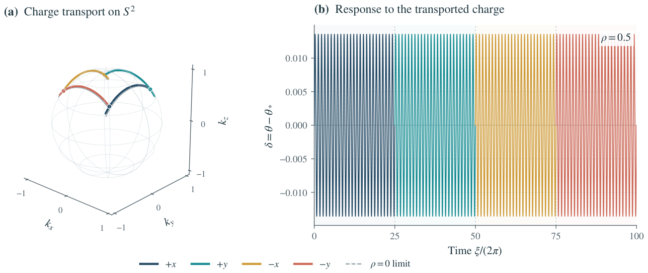
Figure 1. Periodic response and charge at $\rho =+0.5$. Left: the normalized charge $\mathit{k}$ on its unit sphere through the four prescribed blocks; the dashed curve is the zero-charge limiting direction orbit. Right: the response displacement $\delta$ over the same 100 elementary periods. Different charge directions give the same active projection on this symmetric branch, so the response keeps its elementary period while the charge closes after four blocks. Both panels are calculated from the coupled equations.

Figure 1. Periodic response and charge at $\rho =+0.5$. Left: the normalized charge $\mathit{k}$ on its unit sphere through the four prescribed blocks; the dashed curve is the zero-charge limiting direction orbit. Right: the response displacement $\delta$ over the same 100 elementary periods. Different charge directions give the same active projection on this symmetric branch, so the response keeps its elementary period while the charge closes after four blocks. Both panels are calculated from the coupled equations.

4.2. Why Unit-Frequency Compensation Fails Here

At $\nu =1$, the harmonic response and drive have the same frequency. A periodic solution then requires the force to have no component along the resonant mode. Near the reference orbit, the charge force has a definite, nonzero projection on that mode.

Proposition 4.4 

(Resonance obstruction). For the control in Eq. (3.5) and $\nu =1$, there is no sufficiently nearby L-periodic response with nonzero returning traceless charge and noncentral period holonomy.

Proof. 

Charge return gives $\mathit{p}=\rho {\mathit{k}}_{\delta }$. At the reference trajectory, ${\mathit{k}}_0·\mathit{n}=r\left(m{\kappa }_{\mathrm{M}}\right)>0$ on every block. Continuous dependence of transport and the noncentral period axis implies ${\mathit{k}}_{\delta }·\mathit{n}>0$ for sufficiently small uniform response changes. The orbit stays in $0<{\theta }_{*}+\delta <\pi$, so $sin({\theta }_{*}+\delta )>0$ as well. Multiply the exact response equation by $sin\xi$ and integrate through $L=200\pi$. Periodic integration by parts makes its left side vanish, while its right side is

$$0.05\rho {\int }_0^L({\mathit{k}}_{\delta }·\mathit{n})sin({\theta }_{*}+\delta ){sin}^2\xi \mathrm{d}\xi ,$$

(4.12)

which has the sign of nonzero $\rho$ and cannot vanish. This contradiction excludes the proposed orbit. □

At resonance, the periodic linear operator has a mode that its own restoring term cannot balance. Projecting the equation onto that mode removes the entire left-hand side and isolates the corresponding component of the applied force. Here the charge projection and $sin\theta$ retain their signs along every block, so their contributions cannot cancel. Bounded free deviations are thus insufficient for a charged periodic response. The charge force must also satisfy the periodic solvability condition. The choice $\nu =\sqrt{2}$ removes this resonance without changing the reference orbit.

4.3. The Angle Susceptibility

Let ${\mathit{k}}_0$ be the transported reference axis and define

$$F\left(\xi \right)=0.05({\mathit{k}}_0\left(\xi \right)·\mathit{n}\left(\xi \right))sin{\theta }_{*}\left(\xi \right)sin\xi ,y={\left.{\displaystyle \frac{\partial {\delta }_{\rho }}{\partial \rho }}\right|}_{\rho =0}.$$

(4.13)

Differentiating the response equation at zero charge gives the periodic linear problem

$$y^{\prime \prime }+{\nu }^{2}y=F,y\left(L\right)=y\left(0\right),y^{\prime }\left(L\right)=y^{\prime }\left(0\right).$$

(4.14)

The change of the holonomy angle to first order in charge is therefore

$$\begin{array}{cc}\hfill {\chi }_{\alpha }:={\alpha }^{\prime }\left(0\right)& =-{\int }_0^{L}F\left(\xi \right)y\left(\xi \right)\mathrm{d}\xi \hfill \\ \hfill & ={\int }_0^L\left[y^{\prime }{\left(\xi \right)}^2-{\nu }^{2}y{\left(\xi \right)}^2\right]\mathrm{d}\xi =-0.2490598046\dots .\hfill \end{array}$$

(4.15)

The second expression follows by multiplying Eq. (4.14) by y and integrating by parts over a period. Both expressions determine the angle change from the response:

$$\alpha \left(\rho \right)={\alpha }_0+{\chi }_{\alpha }\rho +O\left({\rho }^2\right).$$

(4.16)

For this control, a charge along the period axis lowers the angle; reversing the charge raises it. The sign depends on the frequencies in the forcing. With $F={\sum }_{j\in \mathbb{Z}}{F}_j{e}^{2\pi ij\xi /L}$,

$${\chi }_{\alpha }=-L\sum _{j\in \mathbb{Z}}{\displaystyle \frac{|F_j{|}^2}{{\nu }^2-{(2\pi j/L)}^2}}.$$

(4.17)

Components below and above the response frequency contribute with opposite signs. Their weighted sum is negative for the present drive and compensation. A different prescribed motion can change that sum and hence the susceptibility.

The susceptibility measures how the path’s response to charge is accumulated into a change of the period transport. The function F supplies the force per unit charge, and y gives the displacement it produces. Their integral then determines how that displacement changes the connection sampled along the circuit. The numerical value is fixed once the drive, compensation and coupling are fixed. It can therefore be compared between calculations and experiments using those conditions, without being a universal constant of PODA.

There is also an exact identity along the nonlinear branch. Define the signed quadratic response action

$$\mathcal{J}\left(\rho \right)={\int }_0^L[{\delta }_{\rho }^{\prime 2}-{\nu }^2{\delta }_{\rho }^2]\mathrm{d}\xi .$$

(4.18)

Stationarity of Eq. (4.3) gives

$${\mathcal{J}}^{\prime }\left(\rho \right)=2\rho {\alpha }^{\prime }\left(\rho \right),\mathcal{J}\left(\rho \right)=2\rho \alpha \left(\rho \right)-2{\int }_0^{\rho }\alpha \left(r\right)\mathrm{d}r.$$

(4.19)

The integral $\mathcal{J}$ can have either sign. It is distinct from the positive instantaneous oscillator energy $E=({\delta }^{\prime 2}+{\nu }^2{\delta }^2)/2$, whose work equation is

$$E^{\prime }=0.05{\delta }^{\prime }(\mathit{p}·\mathit{n})sin({\theta }_{*}+\delta )sin\xi .$$

(4.20)

The right-hand side is the power delivered by the charge-dependent force. Energy is exchanged with the prescribed drive during a period even when the response returns at its end.

5. Stability of the Returning Motion

The action also determines the response to small disturbances of the returning motion. Shift the coordinate to $\delta$, set $v={\delta }^{\prime }$, and remove the total derivative ${\displaystyle \frac{\mathrm{d}}{\mathrm{d}\xi }}\left({\theta }_{*}^{\prime }\delta \right)$. The Hamiltonian becomes

$$H={\displaystyle \frac{1}{2}}{v}^2+{\displaystyle \frac{1}{2}}{\nu }^2{\delta }^2+a_{\xi }({\theta }_{*}+\delta ,\xi )\mathit{p}·\mathit{n},\{\delta ,v\}=1,\{p_i,p_j\}=-2{ϵ}_{ijk}{p}_k.$$

(5.1)

The energy balance also records the role of the controls. On each smooth control interval, the Hamilton equations imply

$${\displaystyle \frac{\mathrm{d}H}{\mathrm{d}\xi }}=\left[-0.05sin({\theta }_{*}+\delta ){\theta }_{*}^{\prime }sin\xi -0.05(1-cos({\theta }_{*}+\delta ))cos\xi \right]\mathit{p}·\mathit{n}+a_{\xi }\mathit{p}·{\mathit{n}}^{\prime }.$$

(5.2)

Here the explicit derivative is taken at fixed $\delta ,v,\mathit{p}$. During a constant-direction block the last term vanishes. At an ideal direction switch the Hamiltonian change is $a_{\xi }\mathit{p}·\Delta \mathit{n}=0$, since the switch occurs at $a_{\xi }=0$. The applied drive and potential can still exchange energy with the response during a block. The periodic return is therefore a solution of a driven system; it does not assert autonomous motion of the entire driving apparatus.

The response force and charge rotation are its Hamilton equations. Fixing the nonzero charge length leaves two coordinates on the charge sphere, together with the response position and velocity. The four-dimensional return map on this phase space is real symplectic.

To approach zero charge, keep the normalized direction $\mathit{k}=\mathit{p}/\rho$. In local tangent coordinates $(\delta ,v,k_1,k_2)$, with an oriented orthonormal basis satisfying ${\mathit{e}}_1\times {\mathit{e}}_2=\mathit{k}$, a preserved two-form is represented by

$${\Omega }_{\rho }=\left(\begin{array}{cc}J& 0\\ 0& -\rho J/2\end{array}\right),J=\left(\begin{array}{cc}0& 1\\ -1& 0\end{array}\right).$$

(5.3)

This form is nondegenerate for every nonzero $\rho$. The sphere term vanishes as the charge sphere contracts to a point. The equations for the normalized direction and their linear period map have a regular limit, however, which determines the nearby spectrum. Its direction pair belongs to the limit from nonzero charge; at $\rho =0$, the collapsed charge sphere has no such physical modes.

Proposition 5.1 

(Linear neutral stability near zero charge). If the four numbers

$$e^{i\nu L},e^{-i\nu L},e^{2i{\alpha }_0},e^{-2i{\alpha }_0}$$

(5.4)

are distinct and nonreal, the local periodic branch is linearly neutrally stable on each fixed-charge sphere for all sufficiently small nonzero $\left|\rho \right|$.

Proof. 

At zero charge, response perturbations are independent of charge-direction perturbations and have multipliers $e^{\pm i\nu L}$. The charge direction undergoes the adjoint period rotation, whose tangent multipliers are $e^{\pm 2i{\alpha }_0}$. Response perturbations can affect that rotation, so the limiting period matrix is block triangular; its eigenvalues are nevertheless those in Eq. (5.4).

Choose disjoint neighborhoods of these four simple eigenvalues. Continuity gives one eigenvalue in each neighborhood for sufficiently small $\left|\rho \right|$. For nonzero $\rho$, real symplecticity pairs each eigenvalue $\lambda$ with $1/\overline{\lambda }$. These two values lie in the same neighborhood of the same limiting unit-modulus eigenvalue and must therefore coincide. Hence $\left|\lambda \right|=1$. The eigenvalues remain distinct, so the period matrix is diagonalizable and its powers are bounded. Bounded transport within a period then gives bounded linear perturbations at every time [10]. □

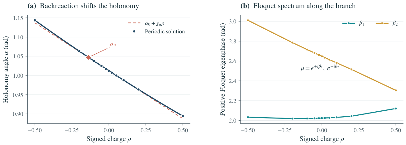
For $\nu =\sqrt{2}$ and $L=200\pi$, the analytic bounds ensure the required separation. Equation (B.2) gives $0<2{\alpha }_0<2\pi /3$, while $1.414<\sqrt{2}<1.415$ places $\nu Lmod2\pi$ in $(4\pi /5,\pi )$. The corresponding positive phase magnitudes are $2.647459319\dots$ and $2.024747133\dots$. On each fixed-charge sphere, small linear disturbances of the response and charge remain bounded, without decay towards the orbit. Nonlinear stability and the accumulated selector displacement are separate questions. In particular, two returning members of the family can have different angles, producing an unfolded phase difference $N\Delta \alpha$ after N cycles. Bounded response and charge disturbances alone therefore give no uniform bound on long-lag event-phase differences. At finite charge, the multipliers are obtained directly from the calculated return matrix.

Figure 2. Holonomy angle and linear stability along the charged branch. Left: the angle from the scalar consistency equation and full coupled shooting; the dashed line is ${\alpha }_0+{\chi }_{\alpha }\rho$. Right: the two positive Floquet eigenphases of the calculated returning motions. Their four multipliers form conjugate pairs and have unit modulus at the displayed points. The stability theorem applies near zero charge; the continuation supplies the finite-charge values.

Figure 2. Holonomy angle and linear stability along the charged branch. Left: the angle from the scalar consistency equation and full coupled shooting; the dashed line is ${\alpha }_0+{\chi }_{\alpha }\rho$. Right: the two positive Floquet eigenphases of the calculated returning motions. Their four multipliers form conjugate pairs and have unit modulus at the displayed points. The stability theorem applies near zero charge; the continuation supplies the finite-charge values.

6. Event Probabilities on the Charged Orbit

The charge changes the response, but their coupled equations contain no selector coordinate. Fixed response and charge data, together with the prescribed controls, determine $W\left(\xi \right)$. An independently prepared Haar selector is carried by this fixed left translation:

$$u\left(\xi \right)=W\left(\xi \right)u_0\sim {\mu }_{\mathrm{Haar}}.$$

(6.1)

In an event partition of the $SU\left(2\right)$ fiber, each cell has its prescribed Haar volume $K_y\left(b\right)$, including the Born choice $K_y(x,s)=Tr\left[{\varrho }_x{E}_y^{\left(s\right)}\right]$. Left translation preserves these marginals at every time, including conditional on the independently prepared base and charge data. Conditioning instead on an earlier outcome restricts the initial selector to one event cell. The correlations arise from the subsequent transport of that restricted set.

The present binary recurrence uses a balanced observation state. Equation (4.11) gives, exactly on the symmetric charged branch,

$${\theta }_{\rho }\left(0\right)={\displaystyle \frac{\pi }{2}},{\theta }_{\rho }\left(NL\right)={\displaystyle \frac{\pi }{2}}.$$

(6.2)

Readings at $NL$ thus share the same balanced base state and drive phase. Choosing another starting point on the periodic path would conjugate the period matrix without changing its angle; the event cells would then need the volumes prescribed by the probability at that point.

Choose a fixed physical anchor $c\in SU\left(2\right)$ in the repeated endpoint frame. The hemisphere record is

$$Y\left(u\right)=sgn\left[{\displaystyle \frac{1}{2}}\Re Tr\left(c^{-1}u\right)\right].$$

(6.3)

This hemisphere is a specified readout partition on the balanced fiber. Its two Haar volumes realize the endpoint probabilities; the transport action alone does not choose its shape or anchor. Away from a balanced endpoint, cells would have to have the corresponding unequal volumes. The recurrence uses only the repeated balanced partition, with the anchor held in the same physical frame.

The anchor and selector transform together under a change of frame, so this sign labels the same physical event in every frame. A fixed rule assigns points on the null boundary. In quaternion coordinates, $u=z_{0}I+i\mathit{z}·\sigma$, $z_0^2+{\left|\mathit{z}\right|}^2=1$, Haar measure is uniform surface measure on the three-sphere. The two hemispheres therefore have equal probability.

Suppose a reading records the sign while retaining the response, charge and selector. The motion then remains on the same charged orbit, with $u_N=W_L^N{u}_0$ after N cycles. For two hemisphere normals separated by angle $\gamma$, projection onto their plane has a uniform polar angle. Their sign tests differ in sectors of total angle $2\gamma$, giving mismatch probability $\gamma /\pi$. Since the principal angle of $W_L^N$ is $arccos[cos(N\alpha \left)\right]$,

$$P_{\mathrm{mis}}(N;\rho )={\displaystyle \frac{1}{\pi }}arccos\left[cos\left(N\alpha \right(\rho \left)\right)\right],\mathbb{E}\left(Y_0{Y}_N\right)=1-2P_{\mathrm{mis}}(N;\rho ).$$

(6.4)

Each record is still balanced; changing the charge changes its correlation with earlier records. To see the distinction, consider the ensemble selected by an initial positive record. Its selectors occupy one hemisphere. Transport preserves the volume of that set while changing its overlap with the hemisphere tested at a later time. The overlap determines the conditional probability for the later record. Combining the initially positive and initially negative ensembles restores the uniform distribution at that time. The same volume-preserving motion can thus preserve every single-record probability while changing the joint distribution of two records. The measured recurrence concerns this joint distribution.

Away from a corner $N\alpha \in \pi \mathbb{Z}$, the first sensitivity is

$${\left.{\displaystyle \frac{\partial P_{\mathrm{mis}}(N;\rho )}{\partial \rho }}\right|}_0={\displaystyle \frac{N{\chi }_{\alpha }}{\pi }}sgn[sin\left(N{\alpha }_0\right)].$$

(6.5)

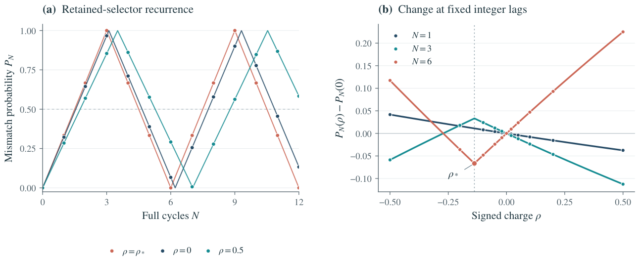
The angle change caused by the response therefore gives a definite change in the mismatch probability. At a fold, the continuous recurrence has two one-sided derivatives. Its extension to real N has an M-shaped pair of peaks over two periods; records sample this curve at integer lags.

Equation (6.4) follows the history preserved by the readings. A readout that moves the response, charge or selector changes the return map and must be included in it. Reversing a coupling direction illustrates the issue: at nonzero $Q_s$, it reverses the charge-dependent force as well as the generator. A two-period readout return derived at zero traceless charge must therefore be recalculated for the charged motion.

6.1. Exact Reversal After Three Charged Cycles

The zero-charge non-Abelian fingerprint takes the event selector close to its antipode after three cycles. The charged branch passes through an angle at which it reaches the antipode exactly. Here resonance refers to a finite-order transport: the response continues to repeat, and the selector returns after several complete cycles. The obstruction at $\nu =1$ concerned a different resonance, between the forcing and the response. On the symmetric branch the antipodal condition requires

$$\beta =m\kappa \left(j_{*}\right)={\displaystyle \frac{\pi }{4}},\kappa \left(j_{*}\right)={\displaystyle \frac{\pi }{100}},{\rho }_{*}=\sqrt{3}{j}_{*}.$$

(6.6)

The last relation follows from $r(\pi /4)=1/\sqrt{3}$. At this point Eq. (4.6) becomes

$$C_{*}={\displaystyle \frac{1}{2}}\left[I+i({\sigma }_x-{\sigma }_y+{\sigma }_z)\right]=exp\left[{\displaystyle \frac{i\pi }{3\sqrt{3}}}({\sigma }_x-{\sigma }_y+{\sigma }_z)\right],C_{*}^3=-I,C_{*}^6=I.$$

(6.7)

Every selector is taken to its antipode after three cycles and restored after six. Apart from the null hemisphere boundary,

$$Y_3=-Y_0,Y_6=Y_0,P_{\mathrm{mis}}(3;{\rho }_{*})=1,P_{\mathrm{mis}}(6;{\rho }_{*})=0.$$

(6.8)

These relations hold for each selector away from the boundary. Haar averaging gives the stated mismatch probabilities while preserving balanced probabilities at every endpoint.

Appendix B proves that this phase condition is reached exactly once on a finite continuation interval, with $-0.12\sqrt{3}<{\rho }_{*}<0$. The central phase per four-block cycle is $4\beta =\pi$. The full group transport is consequently $H_{*}=(-1,C_{*})\in U\left(1\right)\times SU\left(2\right)$ and satisfies $H_{*}^6=(1,I)$. Thus at six cycles both fiber factors return, in addition to the response and charge that return after every cycle. Solving the scalar response condition gives

$${\rho }_{*}=-0.1377922246\dots .$$

(6.9)

A changing charge is not itself an event failure. On this resonant orbit the first block changes the charge by

$$\mathit{p}(\ell )-\mathit{p}\left(0\right)={\displaystyle \frac{2{\rho }_{*}}{\sqrt{3}}}{\mathit{e}}_y\ne 0,P_{\mathrm{mis}}(6;{\rho }_{*})=0.$$

(6.10)

The motion carries a nonzero charge change within the cycle and nevertheless restores every nonboundary hemisphere record after six cycles. An additional impulse from a finite readout interaction would likewise have to be propagated through the response, charge and selector equations before its effect on a record could be determined. The size of such an impulse alone supplies no positive lower bound on the failure probability.

The group identities follow from the phase condition; the response equation determines the charge needed to reach it for this potential and drive. Section 8 gives the change in the two probabilities under a small angle error.

Figure 3. Event recurrence under ideal retained-selector readings. Left: the folded-angle law for the zero-charge orbit, $\rho =+0.5$ and the calculated resonance ${\rho }_{*}$. Markers denote integer lags; the continuous curves display the underlying formula. At resonance the record after three cycles is opposite to the initial record, and the record after six cycles is identical. Right: charge-dependent differences from the zero-charge probabilities at lags 1, 3 and 6, including the cusp at the resonance. Curves follow the scalar consistency equation; discrete comparison points use the full coupled calculation.

Figure 3. Event recurrence under ideal retained-selector readings. Left: the folded-angle law for the zero-charge orbit, $\rho =+0.5$ and the calculated resonance ${\rho }_{*}$. Markers denote integer lags; the continuous curves display the underlying formula. At resonance the record after three cycles is opposite to the initial record, and the record after six cycles is identical. Right: charge-dependent differences from the zero-charge probabilities at lags 1, 3 and 6, including the cusp at the resonance. Curves follow the scalar consistency equation; discrete comparison points use the full coupled calculation.

7. The Calculated Periodic Branch

To find the periodic motion numerically, we adjust four initial coordinates: the response displacement and velocity, and two coordinates for the charge direction. The projection $\mathit{p}·\mathit{n}$ is constant within each block. A scalar integration therefore gives the response and the phase that rotates the charge according to Eq. (3.6). Differentiation gives the shooting Jacobian and four-dimensional return matrix. The initial coordinates are adjusted until the response and charge return; Appendix A gives the details.

The scalar reduction gives an independent calculation of the branch. A sine-series solution of Eqs. (33) and (34) yields 101 points over $-0.5\le \rho \le 0.5$. At the 11 points also calculated by full shooting, the angles agree within $7.4\times {10}^{-14}$. Full shooting at the resonance charge gives an angle within ${10}^{-14}$ of $\pi /3$.

The independently calculated first response gives

$$y\left(0\right)=0,y^{\prime }\left(0\right)=0.02809728566\dots ,{\chi }_{\alpha }=-0.2490598046\dots .$$

(7.1)

The two expressions in Eq. (4.15), evaluated from the angle variation and the quadratic response, agree to $5.5\times {10}^{-13}$. Their common value determines the initial shift of the fingerprint.

Table 1 follows the change to finite charge. Positive $\rho$ lowers the angle and reduces the probability of reversal after three cycles. Negative $\rho$ initially increases it. The probability reaches one at $3\alpha =\pi$ and decreases again beyond that point, as required by the folded-angle law.

At $\rho =+0.1$, the response displacement stays below about $2.80\times {10}^{-3}$ radians, while the mismatch after three cycles changes by about $2.35$ percentage points. The small path change accumulates in the connection integral over each block and in the repeated transport between records. The central phase changes from $4m{\kappa }_{\mathrm{M}}=3.0809663366\dots$ at zero charge to $3.0376848034\dots$ at $\rho =+0.1$. The scalar phase and the non-Abelian angle describe the two fiber factors, each evaluated along the same charged orbit.

The Floquet multipliers of the tabulated motions, including ${\rho }_{*}$, lie on the unit circle to numerical accuracy. They give finite-charge examples of the behavior proved locally near zero; further continuation is needed to determine the intervening and more distant spectrum. Each fingerprint is calculated from its observation trajectory, returning charge and ordered matrix transport. An experimental comparison can measure these quantities alongside the event correlations.

8. Predictions for the Event Records

The response and charge can be calibrated before collecting event pairs. With the drive fixed, the prepared charge determines the observation path. Its connection integral gives the block phase, and the four calibrated coupling directions determine the matrix angle. The event records can then be compared with the correlation predicted from this independently determined motion.

8.1. Parameters and Numerical Fingerprints

For drive amplitude $0.1$, central charge ratio $q/({\mathcal{I}}_S\Omega )=4$ and compensation frequency $\nu =\sqrt{2}$, each signed coupling direction acts for $m=25$ elementary periods. Writing $T_{\mathrm{M}}=2\pi /\Omega$, one four-block cycle lasts $100T_{\mathrm{M}}$, and a lag $N=6$ spans $600T_{\mathrm{M}}$ between ideal readings. A physical sequence must also allow for preparation and any finite readout duration.

The parameter $\rho$ measures the signed traceless charge in units of ${\mathcal{I}}_S\Omega$:

$$Q_s\left(0\right)={\mathcal{I}}_S\Omega \rho T\left(\mathit{h}\right),∥Q_s\left(0\right)∥={\mathcal{I}}_S\Omega \left|\rho \right|.$$

(8.1)

The sign of $\rho$ specifies the orientation relative to the holonomy axis: negative $\rho$ is antiparallel. Before normalization, this conjugate charge has units of action. It has no electric-charge interpretation in the model.

Table 2. Numerical fingerprints of the prescribed realization. Their values are set by its drive, coupling and response potential.

Quantity	Value	Definition and origin
${\kappa }_{\mathrm{M}}$	$0.0308096633663\dots$	Original zero-charge connection integral, Eq. (14).
${\chi }_{\alpha }$	$-0.2490598046\dots$	Derivative ${\alpha }^{\prime }\left(0\right)$ from the periodic response equation and Eq. (39).
${\rho }_{*}$	$-0.1377922246\dots$	Unique charge on the stated continuation interval satisfying $25\kappa \left(j_{*}\right)=\pi /4$ and $j_{*}={\rho }_{*}/\sqrt{3}$.

Table 2. Numerical fingerprints of the prescribed realization. Their values are set by its drive, coupling and response potential.

Quantity	Value	Definition and origin
${\kappa }_{\mathrm{M}}$	$0.0308096633663\dots$	Original zero-charge connection integral, Eq. (14).
${\chi }_{\alpha }$	$-0.2490598046\dots$	Derivative ${\alpha }^{\prime }\left(0\right)$ from the periodic response equation and Eq. (39).
${\rho }_{*}$	$-0.1377922246\dots$	Unique charge on the stated continuation interval satisfying $25\kappa \left(j_{*}\right)=\pi /4$ and $j_{*}={\rho }_{*}/\sqrt{3}$.

The three numbers refer to the same family of motions. The phase fixes its zero-charge member, the susceptibility gives the initial change of the matrix angle, and the resonance charge locates the exact finite-order return. They are constants of this prescribed realization, rather than universal constants.

8.2. The Predicted Sequence and Its Displacement

At ${\rho }_{*}$, the period angle is exactly ${\alpha }_{*}=\pi /3$. Equation (6.4) therefore predicts, at successive complete-cycle lags,

$$\left(P_{\mathrm{mis}}\left(0\right),P_{\mathrm{mis}}\left(1\right),\dots ,P_{\mathrm{mis}}\left(6\right)\right)=\left(0,{\displaystyle \frac{1}{3}},{\displaystyle \frac{2}{3}},1,{\displaystyle \frac{2}{3}},{\displaystyle \frac{1}{3}},0\right).$$

(8.2)

Each entry gives the probability of a sign different from the initial record. After three complete cycles $Y_3=-Y_0$; after six, $Y_6=Y_0$. Either sign still has probability one half at every endpoint, although the signs along one retained history obey these exact relations.

Near the original orbit, $3{\alpha }_0<\pi$ and $\pi <6{\alpha }_0<2\pi$. The third- and sixth-cycle probabilities therefore lie on parts of the folded recurrence with opposite slopes. Equation (6.5) gives

$$\begin{array}{cc}\hfill P_{\mathrm{mis}}(3;\rho )& =0.96674554435\dots -0.23783459417\dots \rho +O\left({\rho }^2\right),\hfill \end{array}$$

(8.3)

$$\begin{array}{cc}\hfill P_{\mathrm{mis}}(6;\rho )& =0.06650891130\dots +0.47566918835\dots \rho +O\left({\rho }^2\right).\hfill \end{array}$$

(8.4)

The slopes are $3{\chi }_{\alpha }/\pi$ at lag three and $-6{\chi }_{\alpha }/\pi$ at lag six. The sixth-cycle slope is thus minus twice the third-cycle slope, with both set by the response susceptibility. At finite charge the nonlinear response gives the values in Table 1.

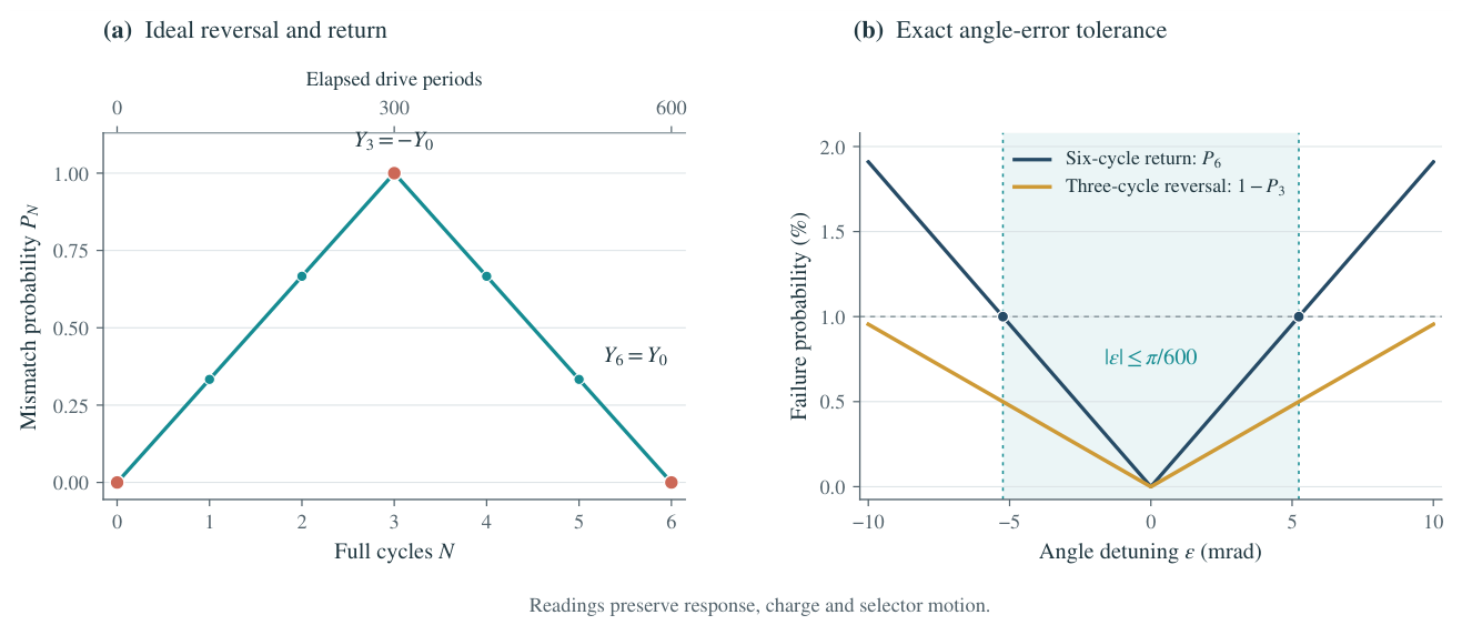
Close to resonance, let the actual period angle be $\alpha =\pi /3+{\epsilon }_{\alpha }$. For $|{\epsilon }_{\alpha }|\le \pi /6$, the folded-angle law gives the exact relations

$$P_{\mathrm{mis}}\left(3\right)=1-{\displaystyle \frac{3|{\epsilon }_{\alpha }|}{\pi }},P_{\mathrm{mis}}\left(6\right)={\displaystyle \frac{6|{\epsilon }_{\alpha }|}{\pi }}=2[1-P_{\mathrm{mis}}\left(3\right)].$$

(8.5)

A fixed angle error $|{\epsilon }_{\alpha }|\le \pi /600$ therefore leaves $P_{\mathrm{mis}}\left(3\right)\ge 0.995$ and $P_{\mathrm{mis}}\left(6\right)\le 0.01$ for the same hemisphere partition. When the transport varies between cycles, its accumulated matrix product replaces the power of a single period matrix.

Figure 4. Exact-return predictions and angle tolerance. Left: the mismatch probabilities at integer lags; the upper axis counts elementary drive periods, with three and six complete cycles lasting $300T_{\mathrm{M}}$ and $600T_{\mathrm{M}}$. Right: third-cycle reversal failures and sixth-cycle return failures for a fixed repeated transport with angle detuning. The shaded interval $|{\epsilon }_{\alpha }|\le \pi /600$ limits these failure probabilities to $0.005$ and $0.01$, respectively. The curves follow Eqs. (61) and (64); preparation and readout errors are not included.

Figure 4. Exact-return predictions and angle tolerance. Left: the mismatch probabilities at integer lags; the upper axis counts elementary drive periods, with three and six complete cycles lasting $300T_{\mathrm{M}}$ and $600T_{\mathrm{M}}$. Right: third-cycle reversal failures and sixth-cycle return failures for a fixed repeated transport with angle detuning. The shaded interval $|{\epsilon }_{\alpha }|\le \pi /600$ limits these failure probabilities to $0.005$ and $0.01$, respectively. The curves follow Eqs. (61) and (64); preparation and readout errors are not included.

8.3. Response and Record Measurements

Measurement of the response $\theta \left(t\right)$ under the known drive $\phi \left(t\right)$ gives the scalar phase

$${\kappa }_{\mathrm{resp}}={\int }_0^{T_{\mathrm{M}}}{\displaystyle \frac{1-cos\theta \left(t\right)}{2}}\dot{\phi }\left(t\right)\mathrm{d}t.$$

(8.6)

On the symmetric branch, $\beta =25{\kappa }_{\mathrm{resp}}$. Equation (4.7) then predicts the angle of the calibrated four-axis transport. A phase-referenced matrix measurement in the common frame provides an independent comparison before the event recurrence is measured. If response measurement disturbs the motion, it must use separately prepared runs under the same controls.

A charge scan also requires calibration of $\rho$. A physical realization must identify the observable corresponding to the action’s charge $Q_s$, as well as the observation coordinate and applied coupling. Each calibrated charge then predicts a response and fingerprint. Fitting $\rho$ from the event data alone would leave this dynamical relation untested.

For each charge setting, the initial data must belong to that setting’s own periodic branch:

$$\theta \left(0\right)={\displaystyle \frac{\pi }{2}},{\theta }^{\prime }\left(0\right)={\theta }_{*}^{\prime }\left(0\right)+{\delta }_{\rho }^{\prime }\left(0\right),\mathit{p}\left(0\right)=\rho \mathit{h}\left({\beta }_{\rho }\right),{\beta }_{\rho }=25\kappa \left(j\left(\rho \right)\right).$$

(8.7)

Both the velocity and charge direction therefore vary along a scan. Holding the old axis ${\mathit{h}}_0$ fixed while changing the charge magnitude would generally leave the returning branch. At resonance the required axis is $(1,-1,1)/\sqrt{3}$, and the calculated initial data are

$${\theta }_{{\rho }_{*}}^{\prime }\left(0\right)=-0.2013265554\dots ,{\mathit{p}}_{{\rho }_{*}}\left(0\right)=0.07955437797\dots (-1,1,-1).$$

(8.8)

The physical angular velocity is $\Omega {\theta }^{\prime }$. These position, velocity and charge values specify the returning motion. Linear neutral stability bounds sufficiently small linear departures, but does not attract other preparations to the branch.

For fixed response and charge data, the initial selector is sampled independently with Haar measure. Read $Y_0$ at the balanced crossing, retain the selector for N complete charged cycles, and then read $Y_N$. Each trial starts with a fresh independent preparation. Repetition at nearby charges measures the probability slopes and resonance together with the associated response changes. The two readings within a trial share one history; different trials are independent.

8.4. Finite Samples and Imperfect Labels

For R independent preparations at the same $(\rho ,N)$, define

$$Z_r={\displaystyle \frac{1-Y_0^{\left(r\right)}{Y}_N^{\left(r\right)}}{2}},{\widehat{P}}_N={\displaystyle \frac{1}{R}}{\displaystyle \sum _{r=1}^R}{Z}_r,{\widehat{C}}_N=1-2{\widehat{P}}_N.$$

(8.9)

The mismatch count for these independent preparations is binomial, with $Var\left({\widehat{P}}_N\right)=P_N(1-P_N)/R$. Overlapping pairs from one long retained sequence are correlated through their shared history. Their count cannot be substituted for R in this variance without accounting for that dependence.

At exact resonance, a failure is $Y_3=Y_0$ at lag three or $Y_6\ne Y_0$ at lag six. If R independent trials at a chosen lag contain no failures, the exact one-sided 95% binomial upper limit obtained by the Clopper–Pearson construction [11] is

$$p_{\mathrm{fail}}^{\mathrm{upper}}=1-0.{05}^{1/R}.$$

(8.10)

For $R=299$ with no failures, this limit is $0.00996915\dots <0.01$ at the chosen lag. Simultaneous limits at lags three and six follow by assigning $0.025$ to each tail with the Bonferroni bound, requiring 368 independent trials per lag. The same preparations may supply both lag readings if the trajectory is retained: the two estimates need not be independent for this bound. Thus a finite sample with no failures places an upper limit on the failure probability; exact zero is the theoretical value.

Finite label accuracy can be treated separately when it leaves the trajectory and partition unchanged. Let the initial and final misclassification probabilities be at most $e_0$ and $e_N$. The mismatch indicator changes only when at least one label is wrong, so a union bound gives

$$|P_N^{\mathrm{obs}}-P_N^{\mathrm{ideal}}|\le e_0+e_N.$$

(8.11)

Label errors may be correlated without invalidating the bound. A disturbance of the response, charge or selector changes the trajectory itself and must be included in the return map.

8.5. What the Comparison Determines

Following the response path, integrated phase, ordered matrix transport and event correlations across a charge scan tests their predicted dependence on one another. A single folded recurrence determines only an angle and admits an effective circle description. The non-Abelian dynamics enters through the measured coupling operations and the charge rotation that changes the response.

With the stated connection and potential, calibrated preparation and retained motion, the response, transport and record statistics are jointly specified. Disagreement with them rules out this realization, while leaving open other dynamics allowed by PODA. Correlation alone cannot distinguish the model from ordinary quantum processes with memory. Independent balanced records correspond to the separately specified reset preparation. The distinguishing prediction here is the quantitative relation between the measured observation response, matrix transport and correlations of retained events.

The observation degrees of freedom used here have a definite extent: a dynamical response path and its conjugate transported charge, a specified connection, and a specified event partition. Finite record formation has not been assigned a pointer action in this paper. Optimizing that interaction, its duration or its control pulses would require a stated class of admissible readouts and the resulting coupled return maps. Neither the periodic resonance nor the present error bounds establish such a global optimum.

9. Conclusion

The traceless charge turns the original M-event response into a family of coupled motions. A periodic response requires the charge to recover the direction that supplied its initial force. For noncentral $SU\left(2\right)$ transport, this is possible only when the initial charge lies along the period axis. The path determines that axis and hence the charge direction that can sustain the path.

At unit compensation frequency, the charge force has a resonant component that prevents a nearby periodic return. Nonresonant compensation admits a unique local branch with bounded linear disturbances of the response and charge at fixed charge length. Its variational equation contains the period angle, whose susceptibility is ${\chi }_{\alpha }=-0.2490598046\dots$ for the chosen control. Four-block symmetry reduces the finite response to a scalar consistency equation. On the interval established in Appendix B, exactly one charge ${\rho }_{*}$ gives $C_{*}^3=-I$ and $C_{*}^6=I$. The approximate reversal and return of the original fingerprint are then exact consequences of the group transport.

Independent Haar preparation preserves the Born marginals throughout the family. The charge changes the path of each retained selector and the relation between its records. Calibration of the response and charge fixes the matrix angle before the records are compared, yielding the probability slopes and exact-return sequence. The angle and sampling bounds give the resolution of that comparison.

Further along a charged branch, returning motions may meet or Floquet multipliers may collide. Such points would mark a change in the response and its recurrence. On the branch considered here, both the observation backreaction and the resulting event correlations follow from the same PODA equations.

References

- C. N. Yang and R. L. Mills, Conservation of isotopic spin and isotopic gauge invariance, Phys. Rev. 96, 191–195 (1954). [CrossRef]
- M. V. Berry, Quantal phase factors accompanying adiabatic changes, Proc. R. Soc. Lond. A 392, 45–57 (1984).
- B. Simon, Holonomy, the quantum adiabatic theorem, and Berry’s phase, Phys. Rev. Lett. 51, 2167–2170 (1983). [CrossRef]
- F. Wilczek and A. Zee, Appearance of gauge structure in simple dynamical systems, Phys. Rev. Lett. 52, 2111–2114 (1984). [CrossRef]
- X. Meng, The Natural Dual-Axis Structure of Observation: Categorical Foundations and Consequences for Quantum Theory, Preprints (2026). [CrossRef]
- X. Meng, Deterministic Quantum Events on a Dual-Axis State Bundle: A Falsifiable Recurrence Test of Single-Event Continuity, Preprints (2026). [CrossRef]
- X. Meng, Non-Abelian M-event dynamics on the physical–observation state bundle, accompanying theoretical manuscript (2026).
- S. K. Wong, Field and particle equations for the classical Yang–Mills field and particles with isotopic spin, Nuovo Cimento A 65, 689–694 (1970). [CrossRef]
- W. Magnus, On the exponential solution of differential equations for a linear operator, Communications on Pure and Applied Mathematics 7(4), 649–673 (1954). [CrossRef]
- G. Floquet, Sur les équations différentielles linéaires à coefficients périodiques, Annales scientifiques de l’École Normale Supérieure, second series, 12, 47–88 (1883). [CrossRef]
- C. J. Clopper and E. S. Pearson, The use of confidence or fiducial limits illustrated in the case of the binomial, Biometrika 26, 404–413 (1934). [CrossRef]
Disclaimer/Publisher’s Note: The statements, opinions and data contained in all publications are solely those of the individual author(s) and contributor(s) and not of MDPI and/or the editor(s). MDPI and/or the editor(s) disclaim responsibility for any injury to people or property resulting from any ideas, methods, instructions or products referred to in the content. |
© 2026 by the authors. Licensee MDPI, Basel, Switzerland. This article is an open access article distributed under the terms and conditions of the Creative Commons Attribution (CC BY) license (http://creativecommons.org/licenses/by/4.0/).
Copyright: This open access article is published under a Creative Commons CC BY 4.0 license, which permit the free download, distribution, and reuse, provided that the author and preprint are cited in any reuse.