How Recursive Causality in Complex Time Generates Shannon Information

Michael Charles Parker; Chris Jeynes; Stuart D. Walker

doi:10.20944/preprints202609.1383.v1

Submitted:

15 September 2026

Posted:

16 September 2026

You are already at the latest version

Abstract

It is well-known that Shannon information may be represented in the usual formalism by points of non-analyticity. We show (assuming that the Second Law of Thermodynamics is taken as axiomatic) that it may also be generated by recursive systems. Trajectories of causality across complex time entail the generation of Shannon information (“entropic purpose”) while recursively causal trajectories also entail the complexification of probability. Causal trajectories across the complex temporal plane, while preserving the distinction between cause and effect (in accordance with the Second Law), also underpin the coherent interplay between the physical effects of acausal Shannon information and purposive agents of causation.

Keywords:

quantitative geometrical thermodynamics

;

QGT

;

determinism

;

agency

;

free-will

;

arctanh

;

complex time

;

complex probability

;

recursion

Subject:

Physical Sciences - Thermodynamics

Introduction

Go, go, go, said the bird: human kind

Cannot bear very much reality.

Time past and time future …

Point to one end, which is always present. T.S. Eliot Burnt Norton I (1936)

Time is central to all our perceptions of reality. In physics, the Second Law of Thermodynamics entails the passage of time. Since Newton, physicists have approximated the representation of time by a simple scalar number, but the poets and philosophers have always known that reality is not so simple. Burnt Norton opens with, “Time present and time past/Are both perhaps present in time future/And time future contained in time past/If all time is eternally present/All time is unredeemable.” But T.S. Eliot knew that “time is redeemable” since Paul of Tarsus commands us to “redeem the time” (ἐξαγοραζόμενοι τὸν καιρόν; Ephesians 5:16; Colossians 4:5). Therefore, we know that Eliot did not believe that “all time is eternally present” (doubtless he also had Queen Elizabeth’s speech in mind: “Swear not by time to come for that thou hast/Misused ere used by times ill-used o’erpast” — Richard III, Act 4 Scene 4). But at least the Second Law establishes a definite asymmetry between past and future.

Causality depends on time: this happening before that. If time is representable by a scalar then causality is straightforward. But we have shown that to unify the description of thermodynamically reversible and irreversible processes using canonical physics it is necessary to complexify time (Parker & Jeynes 2023, PJ23 [1]). In which case the ordering of events (in the complex temporal plane) is no longer trivial and our understanding of causality itself becomes more complicated, so that trajectories across the complex time plane become the basis for a physical description of causality, with the ordering of causal events (governed by the Second Law of Thermodynamics) depending on the topological and Shannon-informational properties (conditioned by the Second Law) of such causal trajectories.

The origin of information has emerged as a fundamental mystery in modern science. Shannon information (that is, information shorn by the communications engineers of all its semantic value) is easy to characterise and measure, using the Shannon metric; but because there is no physical distinction between Shannon information and noise (both being essentially acausal: that is, unpredictable and non-deterministic), extracting the Shannon information from the signal cannot be done ‘objectively’ but requires intelligence (usually represented by a key). Whereas noise as a physical phenomenon is understood to arise from essentially random processes in the universe, Shannon information requires intelligence (of some sort, not necessarily human: we strive to avoid anthropocentricity in physics) both for its creation and for its subsequent processing and exploitation.

We see here, however, an intimate yet also paradoxical relationship between information and causality. On the one hand, Shannon information is essentially acausal in nature: if a (causal) signal can be anticipated then it cannot represent information! But if a signal is not deterministic (that is, its origin and/or arrival cannot be predicted from causal reasoning) then it becomes potentially a source of Shannon information (although if it carries no Shannon information then we call it “noise”). Yet, the mathematical description of causality as expounded authoritatively by John Toll [2] entails the Kramers-Kronig relations, and can be thought to be predicated on the presence of a point of non-analyticity, which is the signature of (acausal) Shannon information! Roughly speaking, this is because causality is equivalent to requiring the associated time-response function to vanish for negative (i.e. earlier) times, which is efficiently described by the Heaviside function. Toll’s treatment in the complexified frequency domain rigorously specifies the conditions for causality and is predicated on a complex dispersion function; as the conjugate to frequency, time is therefore also (implicitly) complexified.

Note that current physics can speak only of “Shannon information”, not of information itself (which of course is what we are really interested in). It is easy to elide the distinction, but such elision must be carefully avoided.

For example, the origins of the informational properties of the DNA molecule currently remain unknown, because to say DNA is ‘created’ by intelligence (of whatever sort) is to say nothing since we cannot say what “intelligence” is; yet it seems vanishingly unlikely to have spontaneously (acausally) arisen as the consequence of a chance sequence of events (see for example Tour et al. 2025 [3]). That is to say, the causal source of the DNA molecule as an information bearing entity is also unknown.

Here we present a new physical account of the origin of Shannon information, offering both a better understanding of the physical conditions required for the generation of such information, and also a deeper insight into what is meant by notions of causality. To repeat, we emphasise the distinction between information (which we personally value) and (impersonal) Shannon information (the objects of the communications engineers). Information is causal in an Aristotelian sense (see Appendix A: information is used by agents to decide what to do, according to their purposes), whereas Shannon information is acausal in a technical sense (being physically indistinguishable from noise).

Any discussion of the origin of information (which we will avoid, noting that instead we are limiting ourselves only to the origin of Shannon information) must touch on the purposes underpinning it (equally to be avoided: we discuss only the impersonal entropic purpose associated with the generation of Shannon information). But discussion of purposes (of any sort) has been regarded as illegitimate in physics since the overturning of Aristotelian teleology in the 17^th century. Aristotle’s (teleological) account of motion was, simply, wrong (for details see Appendix A). And the subsequent Newtonian settlement treated time very simply as a scalar number, a treatment that has persisted through the 20^th century physics revolutions. However, it has turned out that a close discussion of the thermodynamic properties of Shannon information, essential to the treatment of communications efficiency by the engineers (see for example Parker & Walker, 2014 [4]), has led to an elegant relation between the entropy production and the energy of a system requiring the complexification of the whole treatment, including that of time itself (see Eq.23c of PJ23 [ref.1]). And complexified time has certain mathematical properties, exploited by Parker et al. (PJW25a [5]) to define a “purposive” Lagrangian entirely in a two-dimensional temporal plane, which is demonstrated to be valid in canonical physics terms, and which is also shown to represent a system where a quantity known as “entropic purpose” is measurable by the Shannon information generated by the system. Also, the system conforms to a “Principle of Least (Entropic) Purpose” minimising the line integral of the “purposive Lagrangian” along a “causal trajectory”; a Principle completely isomorphic to the Principle of Least Action (minimising the line integral of the Lagrangian along the trajectory).

The creation of Shannon information (which in this “entropic purposive” context can be considered as the quantification of some kind of decision-making process) can only occur in the context of a future-orientated goal (the achievement of some kind of future objective). Note here that entropic purpose is to purpose as Shannon information is to information; and since it is future-orientated we regard the word purpose as appropriate. It is important to note that the concept of a complex temporal plane allows the possibility of multiple possible “causal trajectories” (constrained by the Second Law) connecting points in the complex time plane; such that the choice of which trajectory is adopted by a system as it evolves across the complex temporal plane can be solved by using the calculus of variations (on the Euler-Lagrange equation governing the “purposive Lagrangian”). A far more nuanced approach to the issue of choice (formally stochastic, not deterministic) with the associated information creation is also enabled. This is in contrast to the conventional Newtonian description in scalar (uni-dimensional) time, which represents a more restricted mathematical description with far fewer opportunities for choice. This is the first time since the 17^th century Newtonian revolution that anything like purpose (however cut-down) has been expressible in what may now be regarded as canonical physics terms.

Clearly, causality is closely related to any ideas of temporal trajectories (paths in time). Currently we take as axiomatic that effects cannot precede causes. But how does this work if time is properly to be represented not by a scalar but by a complex number? After all, it is well known that the mathematical comparison of ‘i’ and ‘1’ using the inequality sign (for example) is meaningless. The ordering of numbers on the real number line is well defined, but the ordering of (complex) numbers across the complex plane is not. Aristotle’s idea of motion is clearly faulty, but his analysis of the causes of things is today being re-evaluated (see for example George Ellis, 2023 [6]). See Appendix A on the mediaeval (Aristotelian) approach to causality that underpinned the 17^th century revolution in physics; and on the related discussion of determinism vs. agency.

Synopsis

We reprise the well-known description of points of non-analyticity in spacetime as being an origin of Shannon information, but we show here that another source of Shannon information is that of recursion, this being expressed by the (complex) arctanh function which is meromorphic (that is, also possessing at least one point of non-analyticity in its associated complex plane). The arctanh function being meromorphic for complex arguments underlines that probability itself (previously shown to involve arctanh) is also properly represented by complex numbers, which we show explicitly.

Then we give two physical example systems both resulting in the arctanh function: the first being an idealised case involving only real quantities; the second case being more realistic and resulting in light trajectories following a double logarithmic spiral (DLS) locus.

We discuss various issues, including causality explicitly, its analysis using Hilbert transform theory, as well as its treatment in the context of the complex time plane; and conclude.

Non-Analyticity as an Origin of Shannon Information

We again draw attention to the distinction we make here between information (intrinsically personal) and the (impersonal) Shannon information (SI). Here we limit the discussion to Shannon information.

The definition of Shannon information as involving a point of non-analyticity in spacetime was given in 2010 by Parker & Walker [7] and elaborated more rigorously in 2019 by Parker & Jeynes (PJ19) [8], whose treatment we follow. It is now generally accepted that the mathematical-physical representation of Shannon information formally involves non-analyticity: it used to be thought that Shannon information travels with the group velocity of the wave but Stenner et al. (2005) [9] have shown that the Shannon information (specifically as embodied by the information precursor) travels essentially at the speed of light – which is consistent with the Shannon information here being represented by a point of non-analyticity.

In particular, for a point of non-analyticity in a field Ψ with Euclidean co-ordinates (x,t) in (conventional) Minkowski space-time, then the calculation of the Shannon entropy (S) and Shannon information (I), respectively associated with that point of non-analyticity is given by (simplifying Eqs.1 of [ref.8], and see Eqs.1 of [ref.5]):

\begin{matrix} S = k_{B} \ln c t (1) \end{matrix}

\begin{matrix} I = i k_{B} \ln x (2) \end{matrix}

where the Shannon metric −ρlnρ is used, with the probability ρ ≡ |Ψ|², and as usual k_B is the Boltzmann constant and c is the speed of light. The key thing to notice is that the Eqs.1&2 resulting from the application of the Shannon metric effectively represent a transformation from a Euclidean representation (x,t) of the spacetime point of non-analyticity to a hyperbolic (ln x, ln t) spacetime description. Thus, if we use the symbol q_n as representing a location in hyperbolic spacetime, where n ∈{x, ct}, then Eqs.1&2 can be equivalently represented in hyperbolic spacetime as (see Eq.7a of [ref.5] and Eq.9a of [ref.8]):

\begin{matrix} q_{n} \equiv R \ln \frac{n}{R} (3) \end{matrix}

where the (Euclidean length) scale factor R determines the system length scale, and the Boltzmann constant k_B is not explicitly required since the dimensionality is already appropriate to spacetime (a Minkowski metric is implicit in Eq.3). Thus, we see that a hyperbolic (logarithmic) spacetime geometry is naturally informational. To define a hyperbolic “velocity” normalised to the speed of light c, we may take the differential of the hyperbolic location q_n(T) with respect to some parameter T (assumed here a temporal quantity; see Eq.7c of [ref.5]):

\begin{matrix} q_{n}^{'} \equiv \frac{1}{c} \frac{\partial q_{n}}{\partial T} = R \frac{n^{'}}{c n} (4) \end{matrix}

We see that the hyperbolic velocity

q_{n}^{'}

is dimensionless, and (following the treatment of PJ2021 [10] §7) we find:

\begin{matrix} 0 \leq q_{n}^{'} \leq 1 (5) \end{matrix}

Defining the velocity quantity

q_{n}^{'}

of Eqs.4&5 as the group hyperbolic velocity, then the phase hyperbolic velocity

q_{n}^{' *}

is simply the reciprocal and given by:

\begin{matrix} q_{n}^{' *} = \frac{1}{q_{n}^{'}} (6) \end{matrix}

In which case the phase hyperbolic velocity is bounded by the following inequalities:

\begin{matrix} 1 \leq q_{n}^{' *} \leq \infty (7) \end{matrix}

That is to say, the product of group

q_{n}^{'}

and phase

q_{n}^{' *}

hyperbolic velocities is unity. This is completely isomorphic to the conventional result of kinematics that the product of group (v_g) and phase (v_ϕ) velocities is equal to the square of the speed of light; noting that in natural units (c=1) this would also simply be unity:

\begin{matrix} v_{g} v_{φ} = c^{2} (8) \end{matrix}

Not only is there an isomorphism between the hyperbolic velocities and their kinematic counterparts, there is also an isomorphism between the hyperbolic group velocity

q_{n}^{'}

and the quantity of probability ρ, which has the same properties (indicated by the inequality of the dimensionless Eq.5). Probability is physical! (See ref.13 for a deeper discussion of this particular point.)

Note again: the probability ρ is not the same as the probability amplitude Ψ (frequently seen in quantum mechanics) which must be modulus-squared according to the Born rule: ρ ≡ |Ψ|². However, whereas the Born rule usually ensures that probability is a purely real quantity, it is apparent from the subsequent analysis presented here that there is a strong case to be made that all physical quantities (including probabilities) allow also for complex descriptions.

Recursion as a Generator of Shannon Information

In PJ23 [ref.1] we point out that John Toll [ref.2] explicitly gives a rigorous proof that strict causality (that is, where causes necessarily precede their effects) is logically equivalent to the existence of the (complex) “dispersion relations”, which are ubiquitous as practical constraints in signal processing; so that, in optics (for example), the refractive index necessarily has an imaginary component that is associated with the presence of absorption. It is well-known from quantum mechanics that any particle can be represented as a wave, such that any scattering process must have a representation in terms of a “frequency distribution”, with the corresponding “group” and “phase” velocities. Toll has shown how the real and imaginary parts of the optical dispersion are mutually related via the Kramers–Kronig relations, using the properties of the Hilbert transform. Toll further points out that exactly the same formalism is applicable generally; not only to optics but also to (for example) high-energy particle scattering (citing the “excellent discussion” by Eugene Wigner [11] of the so-called “R-matrix” representation used extensively in Ion Beam Analysis to handle “non-Rutherford” elastic scattering cross-sections [12]).

Quantitative Geometrical Thermodynamics (QGT [ref.8]) shows how meromorphic functions may be used to express information and how holomorphic functions express maximum entropy systems.

Parker et al. (PJW25b [13]) have also previously proved the hyperbolic properties of probability, most notably seen in the hyperbolic sum rule (HSR) which offers the most Bayesian (maximum entropy; MaxEnt) way to add probabilities together with the fewest assumptions; that is, how to properly sum Shannon information without making unacknowledged assumptions. This is in contrast to the conventional sum rule (CSR) of probability theory that explicitly (a priori) excludes the possibility of recursion, and although MaxEnt within its domain of applicability, is found to exhibit a lower entropy than the HSR due to its intrinsic additional constraint. That is to say, the CSR is not as maximum entropy as is the HSR due to its additional inherent assumptions.

The HSR (which is the hyperbolic OR function in probability theory) is also isomorphic to the way that kinematic velocities properly sum together in special relativity. That is to say, given two probabilities ρ₁ and ρ₂, their sum according to the HSR is given by (Eq.12 of [ref.13]):

\begin{matrix} ρ_{1} OR ρ_{2} \equiv HSR (ρ_{1}, ρ_{2}) = \frac{ρ_{1} + ρ_{2}}{1 + ρ_{1} ρ_{2}} (9) \end{matrix}

which is clearly isomorphic to the velocity addition theorem of special relativity w/c=(u/c + v/c)/(1 + uv/c²), where u and v are the kinematic velocities (in co-parallel frames of reference) to be summed and w is the resultant velocity, with c the speed of light as usual. Eq.9 is also isomorphic to the double-angle hyperbolic tangent mathematical identity:

\begin{matrix} \tanh (A + B) = \frac{\tanh A + \tanh B}{1 + \tanh A \tanh B} (10) \end{matrix}

which means that we can identify the hyperbolic tangent of some quantity A with a general probability

ρ

:

\begin{matrix} \tanh A \equiv ρ (11) \end{matrix}

\begin{matrix} A = \tanh^{- 1} ρ (12) \end{matrix}

\begin{matrix} = \frac{1}{2} \ln \frac{1 + ρ}{1 - ρ} (13) \end{matrix}

using the standard identity for tanh^-1.

But considering the whole complex plane, arctanh(z) is meromorphic, with poles at z = ±1. Therefore, since recursion entails the arctanh function which (being meromorphic) in turn entails the existence of points of non-analyticity, recursion entails the generation of Shannon information.

And any functions that nest recursion will generate much Shannon information. We suspect that reality is fractal (that is, not continuously differentiable), and fractal functions (such as the Weierstraß function [14] or the function giving rise to the Mandelbrot set [15]) are well-known even if their use in current physics is not. Functions associated with the Mandelbrot set are also highly recursive, so that if it turns out that they can represent reality as well as the currently conventional (differentiable) complex analysis, then they will also be able to account (in a way currently unavailable) for the Shannon information in real systems.

Complex Probability

Comparison of Eq.13 with Eqs.1&2 suggest that, being logarithmic in nature, the quantity A (characterising the event labelled “A”) is equivalent to some kind of informational term based on the probability ρ. Which is related (but not identical) to the Shannon metric (−ρlnρ). From PJW25b [ref.13] (Eq.4a discussed in Section 3.1) we have the involutive (self-reciprocal) function Σ (defined as Σ(Σ(x)) ≡ x):

\begin{matrix} \bar{ρ} \equiv Σ (ρ) = \frac{1 - ρ}{1 + ρ} (14) \end{matrix}

where

\bar{ρ}

is the inverse probability of ρ, such that

{ρ OR \bar{ρ}} = 1

. But rather than just assuming that

\bar{ρ} = 1 - ρ

(using the involutive function

Σ (ρ) = 1 - ρ

, as employed by Richard Cox [16] and Edwin Jaynes [17]) PJW25b [ref.13] shows that Eq.14 incorporates a fully recursive character to the definition of the inverse probability (noting that it too is MaxEnt: see Appendix A.5.3 of [ref.13]).

Thus, assuming the event “A” occurs with a probability ρ relative to all other possible events that could possibly influence it, means that the quantity A can now also be understood as:

\begin{matrix} A \equiv \frac{1}{2} \ln \frac{1 + ρ}{1 - ρ} = - \frac{1}{2} \ln (Σ (ρ)) = - \frac{1}{2} \ln (\bar{ρ}) (15) \end{matrix}

combining Eqs.13 and 14. Note that ρ is by definition maximally Bayesian (MaxEnt): that is, making the fewest possible assumptions about the natures of all the dependencies (including that of recursion) on other events. Note also that therefore, we can now directly relate A to the information of the inverse probability:

\begin{matrix} 2 A \equiv - \ln (\bar{ρ}) (16) \end{matrix}

What is interesting here is that where Eq.12 indicates that the quantity A is indeed closely associated (via the inverse hyperbolic tangent function) with the probability ρ; yet Eq.15 now indicates that it is also actually equal to (half) the information associated with the inverse probability

\bar{ρ}

! That is to say, A is also equivalently equal to the Shannon information associated with all the events that are not influenced by “A”. Again, this shows the apparently paradoxical relationship between Shannon information and causality, since the event “A” is assumed to occur at some definite point in (complex) time, yet it is defined by an acausal Shannon information associated with all events that have no causal relationship with “A”. Alternatively, we have already stated that the probability ρ is (by definition) maximally Bayesian (MaxEnt; making the fewest possible assumptions about causal relationships with all other events). This therefore implies that the inverse probability

\bar{ρ}

is also maximally Bayesian, making the fewest possible assumptions about the acausal relationships with all other events. Thus, we see that the event “A” is defined by a probability ρ that encapsulates all its causal relationships, but also (equivalently) by its inverse probability

\bar{ρ}

that quantifies all its acausal relationships.

We can therefore also define the inverse quantity,

\bar{A}

:

\begin{matrix} \tanh \bar{A} \equiv \bar{ρ} (17) \end{matrix}

\begin{matrix} \bar{A} = \tanh^{- 1} \bar{ρ} (18) \end{matrix}

\begin{matrix} \bar{A} \equiv \frac{1}{2} \ln \frac{1 + \bar{ρ}}{1 - \bar{ρ}} = - \frac{1}{2} \ln (Σ (\bar{ρ})) = - \frac{1}{2} \ln (ρ) (19) \end{matrix}

In which case, we have:

\begin{matrix} 2 \bar{A} \equiv - \ln (ρ) (20) \end{matrix}

such that the complementary hyperbolic quantities A and

\bar{A}

are each fully characterised either by the probability r associated with a potentially recursive event (“A”) or the information associated with the associated inverse probability

\bar{ρ}

. This is a MaxEnt (maximally Bayesian) result independent of the actual nature of the event “A” and its assigned probability in the absence of any other information (including that of recursion if present).

We now explicitly show how the hyperbolic OR function (the HSR: the Hyperbolic Sum Rule) is consistently treated. In particular, we verify that

{ρ OR \bar{ρ}

} =1. From PJW25b [ref.13] Eq.12:

\begin{matrix} ρ OR \bar{ρ} \equiv HSR (ρ, \bar{ρ}) = \frac{ρ + \bar{ρ}}{1 + ρ \bar{ρ}} (21) \end{matrix}

Noting that the hyperbolic functions (e.g. tanh) are unconditionally well-behaved for complex arguments, we now state a general (complex conjugation) transformation for arbitrary (complex) {A,

\bar{A}

}:

\begin{matrix} A \equiv a + ib and \bar{A} \equiv - a + i b (22) \end{matrix}

where

\bar{A}

is clearly seen to be equivalent to the negative of the complex-conjugate of A. We enquire what are the relations between {a, b} in this particular case. We see that {A,

\bar{A}

} may be characterised by real components {a, −a}, but they also have an imaginary component b (a phase factor which appears to be a free parameter). Phase factors are often easy to ignore (although we also note that b may not be purely imaginary). Considering Eqs.16 & 20, in conjunction with Eqs.22 we can write:

\begin{matrix} ρ = e^{- 2 \bar{A}} = e^{2 a - i 2 b} (23) \end{matrix}

\begin{matrix} \bar{ρ} = e^{- 2 A} = e^{- 2 a - i 2 b} (24) \end{matrix}

The ‘conventional’ sum rule (CSR, see [ref.13]), which doesn’t allow for recursion, is

ρ + \bar{ρ} = 1

, and:

\begin{matrix} ρ + \bar{ρ} = e^{- i 2 b} (e^{2 a} + e^{- 2 a}) {= 2 e}^{- i 2 b} \cosh 2 a (25) \end{matrix}

For small a (such that

\cosh 2 a \to 1

) we must have

b = - (i / 2) \ln 2

in order to ensure

ρ + \bar{ρ} = 1

as required for the CSR. In the general case we must have b = −(i/2) ln⁡(2 cosh⁡2a) to ensure

ρ + \bar{ρ} = 1

. Thus, where the CSR is valid (i.e., without recursion) the quantities A and

\bar{A}

(Eq.22) are purely real (as is conventional).

We are also able to obtain the equivalent result for the hyperbolic OR (HSR) equation of Eq.21; substituting in Eqs.11 & 17 (and substituting Eqs.22 into Eq.26):

\begin{matrix} ρ OR \bar{ρ} \equiv \frac{ρ + \bar{ρ}}{1 + ρ \bar{ρ}} = \frac{\tanh A + \tanh \bar{A}}{1 + \tanh A \tanh \bar{A}} = \tanh (A + \bar{A}) (26) \end{matrix}

\begin{matrix} ρ OR \bar{ρ} \equiv \tanh (a + i b - a + i b) = \tanh (i 2 b) (27) \end{matrix}

which in general is not unity. However, there are various possible values for b to ensure

ρ OR \bar{ρ}

=1:

b = \pm i \infty, \pm π / 8 + N π / 2

(for integer N). Note, there may be a phase associated with the result (that is, it may have a complex argument) but, as already discussed, this is conventionally ignored. For example, using

b = π / 8

we have:

\begin{matrix} ρ OR \bar{ρ} = \tanh (i \frac{π}{4}) = i \tan (\frac{π}{4}) = 1 � e^{i \frac{π}{2}} (28) \end{matrix}

It is clear that once recursion is allowed for, then in general probabilities become complex; in contrast to non-recursive scenarios where probability remains purely real. This indicates the difficulty that has hindered a proper consideration of recursive causality up to now: the necessity for complex probabilities (as well as the requirement for complex time). However, once these conceptual issues have been overcome, the resulting mathematical descriptions are both coherent and compelling.

The involutive function S (Eq.14) coheres well with a hyperbolic definition of probability. That is to say, observing the ‘group’ and ‘phase’ versions of the hyperbolic (and kinematic) velocities, and noting again the mathematical similarities between probability and hyperbolic velocity, if we define an equivalent ‘phase’ version of the hyperbolic probability in isomorphism to Eq.6:

\begin{matrix} ρ^{*} \equiv \frac{1}{ρ} (29) \end{matrix}

and substitute Eq.29 into Eq.15 and using Euler’s identity (e^iπ ≡ −1), we find:

\begin{matrix} A \equiv \frac{1}{2} \ln (\frac{1 + \frac{1}{ρ^{*}}}{1 - \frac{1}{ρ^{*}}}) = \frac{1}{2} \ln \frac{ρ^{*} + 1}{ρ^{*} - 1} = - \frac{1}{2} \ln - (\frac{1 - ρ^{*}}{1 + ρ^{*}}) = - \frac{1}{2} \ln (\frac{1 - ρ^{*}}{1 + ρ^{*}}) + i (N + \frac{1}{2}) π (30) \end{matrix}

Thus, we find that the hyperbolic information A due to the probability r is essentially the same (apart from a constant imaginary term) as the hyperbolic information A* due to the ‘phase’ probability r*:

\begin{matrix} A^{*} \equiv - \frac{1}{2} \ln (\frac{1 - ρ^{*}}{1 + ρ^{*}}) = - \frac{1}{2} \ln (Σ (ρ^{*})) (31) \end{matrix}

That is, A is a hyperbolic information quantity, defined with both ‘group’ and ‘phase’ identities, such that (in logarithmic isomorphism to Eqs.6,8) we have:

\begin{matrix} A = A^{*} + i (N + \frac{1}{2}) π (32) \end{matrix}

that is, the ‘group’ and ‘phase’ probabilities are equally likely. Likewise, the ‘phase’ counterpart of Eq.15 is:

\begin{matrix} A^{*} \equiv - \frac{1}{2} \ln (Σ (ρ^{*})) = - \frac{1}{2} \ln (\bar{ρ^{*}}) (33) \end{matrix}

Therefore, the quantity H (the “self-information” H≡−ln(ρ) is in contrast to −ρ*ln(ρ), which is the Shannon information, that is, the “probability-weighted self-information”) can be interpreted as the unweighted Shannon entropy of the inverse probability

\bar{ρ}

, where H is:

\begin{matrix} H = A + A^{*} = - \frac{1}{2} \ln (\bar{ρ}) - \frac{1}{2} \ln (\bar{ρ^{*}}) = - \ln (\bar{ρ}) (34) \end{matrix}

where we ignore the constant factor

i (N + 1 / 2) π

. Note that “Shannon entropy” is indistinguishable from “Shannon information” (or noise, since Shannon information and noise are also physically indistinguishable). Therefore, H=2A is the self-information of the MaxEnt recursive event “A”.

Example 1: The Optical Cavity

We now consider a physically realisable system that demonstrates an application of the complex HSR analysis. The simplest optical structure is a discontinuity in refractive index (here a slab of glass thickness L – see Figure 1) that causes Fresnel reflections with the Fresnel reflection coefficients r₁, r₂ at the two interfaces. Within the cavity there occurs an infinite regression of reflections, each subsequently diminishing by a factor (less than unity) so that they sum to a finite quantity and maintain conservation of energy.

This device is a beam splitter. And it doesn’t matter whether the “incident” beam is incident from the left (as drawn) or the right: the incident beam is split into reflected/transmitted beams either way. Thus, the device causes beam-splitting. This is a statement which is temporal only by implication: a one-beam “system” is envisaged before the beam-splitter is inserted, and a two-beam system after.

The overall reflectivity r_S due to the optical cavity (singularity or point of non-analyticity) is simply given (see Appendix B, Eq.B.6) by the Hyperbolic Sum Rule (Eq.12 of [ref.13]) of the two Fresnel reflections at the two interfaces either side of the structure (including the round-trip phase):

\begin{matrix} ρ_{Σ} = \frac{ρ_{1} + ρ_{2} e^{i 2 k_{2} L}}{1 + ρ_{1} ρ_{2} e^{i 2 k_{2} L}} (35) \end{matrix}

Now the treatment in Appendix B is idealised in that the refractive index is taken as purely real (no absorption), which is physically possible provided that the incident wave is monochromatic. Of course, such a perfectly monochromatic beam can have no start, that is, this example is acausal – except insofar as the device causes beam-splitting. This highlights the polysemic nature of causality, which has both a clear temporal meaning and also a clear logical meaning.

We have gone to the trouble to discuss the physical details behind the phenomenon of an optical etalon since it highlights some key mathematical-physical attributes of the emergence of information and causality. On the one hand, we first note that the optical etalon features two discontinuities (interfaces) whose impact on a probing ray of light is to add hyperbolically. We note that such hyperbolic behaviour is a signature of the presence of information; and indeed, each interface represents a point of non-analyticity (i.e. a perfect discontinuity) which is itself a fundamental attribute of (Shannon) information as already highlighted. Each interface on its own introduces a reflection ρ₁ and ρ₂, respectively, but they can be combined together to create a single reflection ρ_Σ as if the two individual reflections were a single reflection. We can even imagine concatenating multiple more similar optical interfaces, which can be lumped together and considered as a single optical phenomenon, via the addition rule seen in the multiple angle rule of the hyperbolic tangent function:

\begin{matrix} \tanh [A + B + C] \equiv \frac{\tanh A + \tanh (B + C)}{1 + \tanh A \tanh (B + C)} (36) \end{matrix}

From a causality aspect, we first note that the analysis to derive Eq.35 via an infinite regression of reflections is intrinsically causal in nature, since we invoke a notional wave impinging the cavity at some initial point in time, and then we track the subsequent multiple reflections, which we sum. However, it’s noteworthy that were we to repeat the analysis, but this time considering a ray entering from the other side of the etalon (travelling towards the left) we achieve exactly the same result of Eq.35. On the one hand, this is perhaps merely a result of the lateral symmetry of the geometrical structure. But it’s interesting to note that Eq.35 can be derived using either ‘causal’ argument; that is to say, although the argumentation to justify Eq.35 is highly causal (see Appendix B), the final result is essentially acausal (and is essentially independent of time) since the actual ‘causality’ is ambiguous! Thus, the intrinsically acausal nature of Shannon information is confirmed.

Example 2: The Graded Index (GRIN) Cavity

We now extend the analysis to another etalon geometry that also obeys the (complex) HSR (hyperbolic sum rule). However, in this case, the etalon also exhibits attenuation (absorption) and we also assume that it has a circular geometry (in plan view; see Figure 2) so that it could also represent an optical ring resonator (RR) structure. The key motivation for considering this GRIN cavity example is that a notional light ray follows a logarithmic spiral trajectory as it circles around towards the centre of the system. The RR geometry also allows for an alternative logarithmic spiral trajectory for a light ray (i.e. the light enters the RR at a different input location) so that, together, the two optical trajectories together form a double logarithmic spiral (DLS), which is a fundamental Maximum Entropy (MaxEnt) holomorphic trajectory in QGT [ref.8], and which also is the trajectory associated with a trajectory across the complex temporal plane that accords with the Principle of Least Entropic Purpose [ref.5]. That is to say, the (spatial) DLS optical trajectory across the GRIN cavity is isomorphic to the purposive DLS across the complex temporal plane.

The HSR for a comparable GRIN cavity is derived in Appendix C (Eq.C.9). The structure is designed to constrict (the two faces get closer together) along the longitudinal axis of the etalon, such that the width of the etalon reduces exponentially with (recursive) bounce number m as:

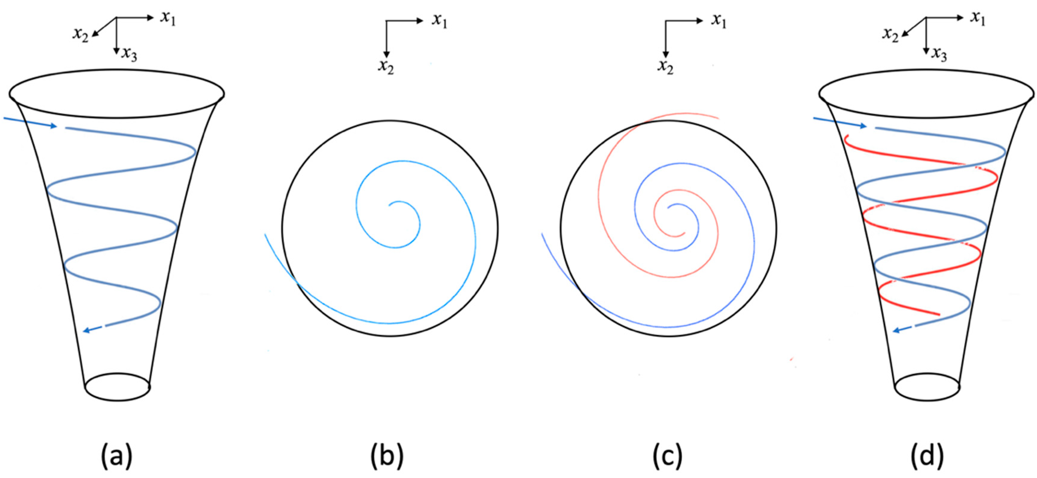
\begin{matrix} L = α^{m} L_{0} = L_{0} e^{- m \ln (1 / α)} (37) \end{matrix}

This Example 2 introduces absorption (and a complex refractive index) explicitly, making it applicable to real signals (which cannot be monochromatic by Fourier’s Theorem since they must have a start and/or end). Figure 2a shows a schematic of such an absorbing optical etalon with circular geometry (with a plan view in Fig.2b) with a logarithmic spiral trajectory for the light (in blue) as it reflects down the waveguiding geometry. We adopt in Figure 2 an orthogonal cartesian co-ordinate system for the geometry, with x₁ and x₂ acting as the transverse axes alongside the x₃ longitudinal axis. The key thing to note is that the blue trajectory can be described parametrically as a function of the longitudinal axis x₃, such that we have expressions for the x₁ and x₂ co-ordinates (as a function of x₃) for the blue light ray:

\begin{matrix} l_{blue} (x_{3}) = \frac{L_{0}}{2} e^{- Λ x_{3}} \cos k x_{3} {\hat{\underline{x}}}_{1} + \frac{L_{0}}{2} e^{- Λ x_{3}} \sin k x_{3} {\hat{\underline{x}}}_{2} (38) \end{matrix}

The point being that comparing equations Eqs.37 & 38, we see that the parameter m (for the depth or longitudinal length of the funnel structure) is equivalent to the x₃ axis, and the logarithmic decay parameter L is equivalent to −lna, while the wavenumber is given by

k \equiv 2 n_{2}^{'} k_{0}

.

We now introduce the ‘ambiguity’ of the alternative ‘face’ at which the light can enter into the optical etalon. This is shown in Figure 2c, where the red coloured trajectory indicates such an alternative trajectory, with the two trajectories (red and blue) showing a double logarithmic spiral (DLS). Figure 2d shows the side-view of such a DLS trajectory as it spirals downwards towards the centre of the circular etalon.

The parametric equations for the red trajectory are simply given by:

\begin{matrix} l_{red} (x_{3}) = \frac{L_{0}}{2} e^{- Λ x_{3}} \sin k x_{3} {\hat{\underline{x}}}_{1} - \frac{L_{0}}{2} e^{- Λ x_{3}} \cos k x_{3} {\hat{\underline{x}}}_{2} (39) \end{matrix}

Together, the two trajectories can be combined as follows to create an overall holomorphic DLS trajectory:

\begin{matrix} Σ = l_{blue} + i l_{red} = \frac{L_{0}}{2} e^{- Λ x_{3}} e^{i k x_{3}} {\hat{\underline{x}}}_{1} - i \frac{L_{0}}{2} e^{- Λ x_{3}} e^{i k x_{3}} {\hat{\underline{x}}}_{2} (40) \end{matrix}

As shown in App.B of ref.[8] (Eqs.B.24 onward) the holomorphic DLS represents the fundamental MaxEnt trajectory (the fundamental eigenvector of the entropic Hamiltonian), and is seen everywhere, not only in nature, but also as a fundamental feature of the Mandelbrot set. As discussed in ref.[5] the DLS also represents the fundamental purposive (causal) trajectory associated with the generation of Shannon information.

Causality in Complex Time

What causes the (acausal) "Shannon information"? The point is that information is causal but Shannon information is acausal! This is precisely why we need here to maintain our strict distinction between them.

If I speak to you on the telephone I put my thoughts into words which my handset turns into electrical signals, and which your handset turns back into the words you hear (and hopefully understand). I (the agent) cause the information (my personal words) which the apparatus converts first to Shannon information (the impersonal electrical signals) and then converts back into information (the words you hear). Of course, these conversions are technically non-trivial.

Now, if I merely say “blah blah blah” to you, then the information that the Shannon information points to is simply meaningless (just as the Shannon information itself also is, per se). The apparatus that converts the information into Shannon information, does so entirely impersonally (that is, irrespective of how meaningful the information really is).

In itself, Shannon information is acausal (being indistinguishable per se from noise), but of course it is generated (caused) by the actions of the agent (which in this case is the telephone apparatus). Physics may treat Shannon information but is currently entirely unable to treat information; although it may be that information per se is treatable physically in principle: Terrence Deacon (2011 [18]) has sketched a way for molecules to display (vestigial) purposes, but this cannot yet be articulated satisfactorily in canonical physical terms.

As an example, which does not initially distinguish the “Shannon information” from the “noise” (as communications systems do), consider a “Bénard convection” apparatus [19]. This has not yet been analysed in QGT terms, but we expect such a system to have a non-zero entropic purpose: that is, it will generate Shannon information (as well as noise: see PJW25a [ref.5]). And yet Bénard convection is fully deterministic! That is, we expect that the generated Shannon information (which is acausal, being physically indistinguishable from noise) can entail a determined final state. But in other cases (such as, for example, the foraging gannets studied by James Grecian et al. [20] that somehow take advantage of the “Lagrangian coherent structures”, usefully reviewed by Sergey Prants [21]) the final state is not determined (the bird may or may not succeed in finding food and surviving). That is, Shannon information may or may not be associated with determinism: it is neither intrinsically deterministic, nor intrinsically non-deterministic.

However, rather than having undirected physical effects (degradation, decay and disorder) as is often suggested in interpretations of the 2^nd Law, we have shown that Shannon information characterises the causation of ordered (and maybe even deterministic) effects on physical systems. It is of course well-known now (notably through Ilya Prigogine’s work [22]) that the flow of entropy may generate ordered systems (such as “Bénard convection” [ref.19] or cyclones [23]).

Up to now, discussions of causality have implicitly assumed a linear (scalar) basis for time, and John Toll’s influential paper on the mathematics of a ‘causal’ system does not overturn this assumption (although it is not dependent on it). Toll’s analysis is based on (complex) Fourier theory in the complex frequency domain, where he shows that the Fourier transform (i.e. frequency distribution) of any causal system has real and imaginary components that are Hilbert transforms of each other. Thus, he argues that the signature of a causal system is the Hilbert transform relationship between the real and imaginary frequency distributions describing the system. This is most clearly seen in the Kramers-Kronig “dispersion relations” (which can be interpreted for refractive index as the causal response – that is, how the electron density of the composition molecules reacts to the excitation of incoming photons).

However, the Fourier mathematics is equally valid for an anti-causal excitation, due to a wave arguably travelling from the future back into the past. The Hilbert transform relationship, based as it is on the Heaviside step function, doesn’t unambiguously distinguish between causal (forward travelling) and anti-causal (backward travelling) temporal excitations. That is to say, the point of non-analyticity in time associated with the Heaviside step function is located at the same instance of time for “causal” or “anti-causal” phenomena.

But such a point of non-analyticity can also be clearly understood to occur in the complex temporal plane as a feature of a meromorphic function. We have already indicated that a point of non-analyticity is the source of Shannon information; but Toll’s analysis shows that it is also a signature of causality (or anti-causality) according to his Hilbert transform treatment. Appendix D shows how a Hilbert transform treatment of the HSR (using the etalon as a physical example) accords with Toll’s treatment, even though it is acausal.

Thus, we see that Toll’s analysis offers a credible mathematical description for causality precisely because it implicitly utilises an information-bearing function, with a localised quantity of information at a specific location in time, which has a physical, ‘causative’ effect. But there remains ambiguity between causality and anti-causality (and acausality is precisely where the arrow of time is undetermined).

Of course, this now accentuates the insufficiency of a concept such as “cause precedes effect” in the context of complex time. Instead we consider the trajectory time T along a causal trajectory across the complex temporal plane (established by PJW25a [ref.5]), which is scalar and uni-directional. In this case, we can see that the causal trajectory T is equivalent to the former Newtonian description of time. Causal events associated with the trajectory (corresponding to points of non-analyticity in the complex time plane) are ordered in a well-defined way giving meaning to the conventional notions of “cause and effect”. The entropic purpose of the trajectory also corresponds to the summation of all the Shannon information encountered along the way and remains future-orientated. In particular, the causal events continue to be associated with points of non-analyticity located at points along the temporal trajectory, such that Toll’s Hilbert transform approach also continues to be valid in its contribution towards a fuller description of causality.

The picture of recursion in such a set-up can also now be understood to be described by a spiralling trajectory across the complex time plane, i.e. a locus corresponding to the DLS. In particular, with reference to the spatial trajectory of a light ray in the absorptive (funnel-like) ring-resonator structure (Figure 2c), the light ‘bounces’ around the faces of the system in a recursive fashion. Similarly, a temporal spiral in the complex temporal plane also exhibits recursive behaviour as it ‘bounces’ around in complex time; although, for the ‘unwrapped and straightened-out’ trajectory such recursion isn’t so obvious. Yet, in complex time it is clearly seen, and also associated with the generation of entropy (or indeed Shannon information) as per the principle of least entropic purpose.

Discussion

Being massless, photons are also timeless so that the Second Law cannot apply directly. Therefore, the apparent ambiguity between the “causal” and “acausal” (time reversal) behaviour of the simple cavity is not real. It is only when we (massive beings) are involved, observing the behaviour of the photons (including the time lapse between turning on the light and seeing its reflection), that it occurs to us to speak of “causality” in this sense. It is interesting that John Toll’s analysis ([ref.2]; showing that the Kramers-Kronig relations entail causality – defined as causes preceding the events they cause) entirely avoids the discussion of time (and the d/dt operator) even though time is implicit in causality.

In this same context it is also interesting that the R-matrix method for calculating elastic particle scattering [ref.12] is also timeless in that the interaction (of massive particles in this case) is reversible and elastic, intrinsically with zero entropy production; but the process is still (similarly) causal. Actually, a detailed entropic analysis has not been done: that is, we expect entropy increase according to the Second Law (during the scattering process) to be negligible in these high energy reactions. (Obviously, the momentum transfer to the scattered nucleus, and the electronic energy losses of the fast particles are all carefully accounted for in the current canonical treatment.)

Therefore the optical devices of the two Examples are helpful to direct our attention to what is important: a) the recursion involving an infinite sum (which may be represented as a non-analyticity); or b) the entropy necessarily created by the device per se (for example, beam-splitters make two beams from one, which increases the entropy); and c) the entropy necessarily generated by the device (since any real device must have finite – non-zero – absorption, by the Kramers-Kronig relations), which may be in the form of either noise or (the physically indistinguishable) Shannon information (or a mixture of them). Note that a) and b) may be two ways of describing the same thing.

We see here an apparent contradiction between Shannon information (which is acausal) being generated by (causal) purposive trajectories; however, such a description is now seen to be physically coherent when considered from the perspective of the complex time plane. In developing this thermodynamical theory of information-based causality, based on the presence and effect of Shannon information, we have built on Landauer’s idea that “Information is physical”[24], also that Shannon information must have physical effects (since any event will have an effect, whatever the real cause of the event itself). So that whether or not the Shannon information itself is “causal”, its presence in the purposive trajectories is causal. We recall that “causality” may be present without noise production; that is, the Second Law and causality per se are not to be identified, even though both are predicated on the passage of time.

We need to point out that an obvious (“easy”) calculation for the proportion of noise to Shannon information is in the case of communications channels, which are designed to keep the Shannon information identifiable in the presence of noise. So the Shannon capacity theorem (also known as the Shannon-Hartley Theorem) [25] states:

\begin{matrix} C = B * \log_{2} (1 + \frac{S}{N}) (25) \end{matrix}

where C is channel capacity (b/s), B is the bandwidth (Hz), S is the signal energy (the energy associated with the actual Shannon information) and N is the energy of the noise. Modern communications channels have optical S/N ratio values >20 dB with channel capacities >10¹² b/s and bandwidths >10¹³ Hz (the relation between S/N and the “optical S/N ratio” - OSNR - is given in Essiambre et al., 2010 [26]; Eq.36). Such optical fibre-based channels have very low losses of down to 0.2dB/km (the fundamental Rayleigh scattering limit for silica fibres at a wavelength of 1.55 μm) which means that repeater spacings can be ~100 km. It turns out that non-linear effects set a fundamental limit [27] on the channel capacity of single-mode (thin!) optical fibres of about 2×10¹⁴ b/s.

Parker et al., 2025 [ref.5] have shown that the “entropic purpose” of a system is measured by the Shannon information it creates, but so far no system has been described so closely as to be able to say how much of its entropy production is “Shannon information”, not even for such a simple and well-known system as the “cells” created in Bénard convection (see for example Cerisier et al., 2005 [ref.19]), which we expect to have a non-zero “entropic purpose” by this measure.

Conclusions

Causality involves the ordering of time (causes must precede their effects). But this ordering is ambiguous in the complex temporal plane, an ambiguity resolved by the Second Law. Purposive (complex) trajectories (which are per se causal) conform to the Principle of Least Entropic Purpose (and to the 2^nd Law). Crucially, they preserve the distinction between cause and effect, which is otherwise lost in the complex time plane.

Recursive systems and structures also exhibit ambiguity in the distinction between cause and effect; yet we have shown that such recursiveness generates Shannon information because it is associated (via the Hyperbolic Sum Rule, HSR) with the complex arctanh function, which is meromorphic. This is in contrast to non-recursive systems which are associated with the Conventional Sum Rule (CSR) which doesn’t have any poles in the complex time plane. Here we have also shown that that, just as the dispersion (Kramers-Kronig) relations must be complex, so also must be the arguments of the HSR. Probability must therefore also be treated as intrinsically complex (particularly for recursive systems) just like time itself.

In addition, rather than having undirected physical effects (degradation, decay and disorder) as is often suggested by interpretations of the 2nd Law, we have shown that Shannon information is an agent of causation of ordered (and maybe even deterministic) effects on physical systems. It is of course well-known now (notably through Ilya Prigogine’s work) that the flow of entropy may generate ordered systems.

Shannon information is therefore created in at least two ways: i) by points of non-analyticity in spacetime; ii) and by recursive structures. The first of these, at its simplest, is associated with particles, which are described as point-mass or point-charge entities surrounded by an inverse square-law field; the point of non-analyticity being associated with the exact centre of such a particle. The second of these sources of Shannon information, the recursive structure, can either be a physically geometric configuration (e.g. the optical etalon), a logical structure, or a system which features recursion. It may be that information can be created by other ways (still to be determined) but it is clear that many geometric features of the natural world, as well as many features of human society and the animal and plant worlds, with respect to their organisation, interactions and descriptions are recursive. This makes them highly informational structures, which can exhibit intrinsic purpose and act as agents of causation in the universe.

Overall, we have shown how complexification of both time and probability enables us to provide an information-based description of recursive causality that coheres well with existing causality theory.

Author Contributions

Conceptualization and analysis, M.C.P.; writing—original draft preparation, C.J.; writing—review and editing, M.C.P., C.J., S.D.W. All authors have read and agreed to the published version of the manuscript.

Funding

This research received no external funding.

Data Availability Statement

The original contributions presented in this study are included in the article. Further inquiries can be directed to the corresponding author.

Acknowledgements: We thank V.F.Jeynes for reminding us of T.S.Eliot’s poem

Conflicts of Interest

The authors declare no conflict of interest.

Appendix A. Aristotelian Causality

The European “Enlightenment” was led by humanists such as Desiderius Erasmus (c.1466-1536) and Francis Bacon (1561-1626), and it was customary then for the scholastic philosophers (the “schoolmen”) to be derided, so that a “dunce” was a follower of the “Subtle Doctor” (the very influential Duns Scotus, c.1265-1308).

However, the “schoolmen” of the 12^th-16^th centuries made great advances in both logic and physics, from Robert Grosseteste’s (c.1175-c.1253) first (very popular) Commentary on Aristotle’s Posterior Analytics, to (naming only a few): Roger Bacon (c.1220-c.1292), Thomas Aquinas (c.1225-1274), William of Ockham (c.1287-1347), Jean Buridan (c.1301-c.1360), Albert of Saxony (c.1320-1390), Nicole Oresme (1325-1382), John Wyclif (c.1328-1384), Nicolas of Cusa (1401-1464), Francisco Suárez (1548-1617) and Robert Bellarmine (1542-1621).

We must also mention the 16^th century Reformation, where the attack on the temporal hegemony of the Roman Church was led (reluctantly) by Martin Luther (1483-1546) and countered by the Council of Trent (1545-1563). Aquinas was recognised as a “Doctor of the Church” in 1567 by the then pope, and Thomas’ masterpiece Summa Theologiae was honoured at the Tridentine Council. We could say that Trent was responsible (through Thomas Aquinas) for the establishment of Aristotelianism in the Roman dogma of which Galileo fell foul.

Pietro Redondi[28] has shown that Galileo’s condemnation in 1633 was probably strongly influenced by the Jesuit opposition to his very popular 1623 book Il Saggiatore on account of its (very modern) doctrine of matter, which they recognised as being opposed to the Aristotelian doctrine of substance that underpinned the Roman (Thomist) explanation of the Eucharist (Ferrone & Firpo’s [29] criticism of Redondi’s argument modifies but does not destroy it). The bread and wine were thought to be transubstantiated (this word was used by the 4^th Lateran Council, 1215) into Christ’s body and blood (where the persisting breadness of the bread and wineness of the wine were “accidental” – an Aristotelian category). Galileo’s account of matter was certainly inconsistent with the Thomist one (which the Council of Trent positively reaffirmed).

There seems now to be a consensus that Bishop Étienne Tempier’s Condemnation of 219 Aristotelian and Averroist doctrines in 1277 (see Hans Thijssen, 2003 [30]) stimulated the critical approach to Aristotle by the later scholars (like Ockham and Duns Scotus) that provided a foundation for the 17^th century “scientific revolution”: the great Pierre Duhem went so far as to suggest that 1277 could be thought of as “a date for the birth of modern science” (quoted dismissively by Alexandre Koyré [31]). Tempier’s Condemnation also implicated Aquinas, whose work was aimed at making Christian sense of (the pagan) Aristotle. Hans Küng [32] has explained that Tempier’s inclusion of Thomistic propositions severely damaged Thomas Aquinas' reputation for many years.

The “scientific revolution” of the 17^th century was led (among others) by Galileo Galilei (1564-1642) and Isaac Newton (1643-1727). But this did not happen without precedent! Stanley Jaki [33] has pointed out that Jean Buridan’s commentary on Aristotle’s view of the heavens [34] was later read by Galileo, who quoted from it nearly word for word to refute Aristotle’s explanation of projectile motion (as noted by E.A. Moody in his Introduction to Buridan’s Quaestiones [ref.34]. Moreover, Galileo read Albert of Saxony’s Quaestiones de caelo et mundo, a slightly modified version of Buridan’s Quaestiones, in the collection of mediaeval writings in physics published by G. Lockert in Paris in 1516 and 1518 (Moody [35]). In the place of the Aristotelian insistence on the existence of intelligences that move the planets and stars in their spheres Buridan has the concept of “impetus” whereby a motion can be impressed on a body. The whole context in which projectile motion is discussed in mediaeval times is given by Marshall Clagett [36], and Buridan’s works were widely read: for example, Buridan’s works in physics were required reading when Copernicus was a student at Cracow [ref.35].

Thus, Galileo was aware of Buridan’s impetus theory, although he discovered the law of free fall independently and accidentally, as Stillman Drake argues [37]: Drake also shows that although the “Merton calculators” knew essentially the same result (the “mean speed theorem”, also known as the “Merton rule”, of which Oresme had given a geometrical proof [38]) and their results were then well-known, they did not apply them to free fall problems. Drake claims that “Galileo’s conclusion” (published in his Discourses of Two New Sciences of 1638) on carrying out a certain calculation recorded in a document dated c.1604 “is in a way the starting point of the modern era in physics” [ref.37]. Drake also points out [39] that Galileo used the Eudoxian theory of proportion (from Book 5 of Euclid) rather than the Pythagorian theory (from Book 7): the difference is in how incommensurables are handled (rational and irrational numbers are incommensurate, but the Eudoxian theory allowed ratios of them – see also Ian Mueller [40]). Drake comments that “There was nothing wrong with any of those theories of proportion, but they were far from being all the same thing; nor would any of them have been strictly deducible from any other. The rigorous arithmetization of the continuum by a complete revision of the classical concept of number enables us now to deduce the Pythagorean theory of proportion from the Eudoxian; but to Euclid, the former by no means appeared as a mere special case of the latter” (see note 1 of [ref.39]). The point here of course is that the mediaevals (following Aristotle) insisted on quantising speed so that Galileo’s “continuous-motion hypothesis, which incidentally was promptly rejected by Descartes” [ref.39] was a challenge to the Aristotelians (and recognised as such, as Redondi [ref.28] points out). We also comment, parenthetically, that although Galileo is widely thought to have been wedded to the naturalness of circular motion, Stillman Drake also shows this to be an error: it seems that Galileo recognised both linear and angular momentum [41].

John Maynard Keynes famously said “Newton was not the first [thinker] of the age of reason. He was the last of the magicians …”[42] in an essay intended to be read at the proposed 1942 Royal Society Tercentenary celebration of Newton’s birth, this was postponed to 1946 (after WW2: the essay was read by his brother, Sir Geoffrey Keynes since Keynes himself had died three months earlier). Newton, Galileo and the others were all brought up and deeply influenced by the schoolmen, notwithstanding their Herculean struggles to free themselves from Aristotelianism. Nevertheless, we today have internalised Newton’s (then entirely new and seminal) treatment of time and differentiation (even though we now essentially use Leibniz’ formalism) to the extent that it is hard to think otherwise regarding causality.

But Aristotle’s treatment of causality is much richer than Newton’s (for all that Newton’s has proved exceptionally powerful). For example, one chapter of William of Ockham’s Summa Logicae is titled: “How are principles said to be the causes of the conclusion?” (Ch.15 of Summa Logicae Part III Tractate II). The translator, John Longeway, says of this: “How are causal principles rooted in the real natures of things, and how is it possible to know them? How does functionality occur in the natural world? What is the nature and function of scientific knowledge, and how is it related to knowledge of a more ordinary sort? All these questions are dealt with from the standpoint of a scientific realism rooted in the conviction that scientific explanation captures the causal structure of reality” [43].

Now the Scholastics were Aristotelian to the extent that they thought (erroneously) that correct logic was necessarily syllogistic: Ockham even says explicitly, “every demonstration is a syllogism” (Summa Logicae III-II ch.2 [ref.43]). And Aristotle’s Posterior Analytics was commented heavily by all the major thinkers. For example, Longeway is explicit that Ockham’s Summa Logicae “depends on and purports to interpret” it [ref.43], explaining that “Ockham focuses on [the] problem … how does one demonstrate an attribute of a subject?”. It must be said that this discussion is arcane and highly technical: Longeway lists 5 different types of attribute and 7 different sorts of demonstration in the Summa Logicae, and no less than four (!) ways in which something can “be per se”! In the hands of the Scholastics, syllogistic logic was developed far beyond what even Aristotle achieved. Nevertheless it is still only a first-order logic, proved complete by Kurt Gödel in 1929 (Gödel proved axiomatic arithmetic incomplete in 1931, to the dismay of David Hilbert among others).

Kedar & Hon [44] argue that “in the process of making the concept of law of nature, forms and laws were coherently used in theories of natural causation”, discussing Robert Grosseteste and Roger Bacon. They largely accept the “far reaching statement [of Alastair Crombie [45]] that with Grosseteste ‘Oxford became the first centre of the methodological revolution with which modern science began’”. Ori Belkind [46] has also discussed how the idea of “Law of Nature” was understood by Roger Bacon, and how it developed into its Cartesian expression in the 17^th century out of the Aristotelian idea of “Natural Principle” (understood as inherent in the nature of the thing). The point here is that Natural Principles are taken to be innate to substances and arise from their natures, while Laws of Nature are external and imposed from without. Belkind “argues that during the late Middle Ages and in the Early Modern era, philosophers began to disentangle substantial actions from the nature of substances”. On Bacon, Belkind says, “it seems as if Roger Bacon’s [framing of Law of Nature] is dependent on a reformulation of Aristotelian categories of natural causation”. And note that this discussion of causality by the scholastics and the early moderns did not depend on any simple (Newtonian) view of time. In this context it is also worth pointing out that John Toll’s (modern, [ref.2]) treatment of causality (in terms equivalent to the Kramers-Kronig relations) neither mentions time explicitly, nor uses the d/dt operator.

On the issue of causality, Paul Forman [47] claims to present “overwhelming evidence that in the years after the end of the First World War but before the development of an acausal quantum mechanics … large numbers of German physicists, for reasons only incidentally related to developments in their own discipline, distanced themselves from, or explicitly repudiated, causality in physics”. We think that Forman demonstrates that the postwar “intellectual environment” was favourable to work that was not committed to the old notions of what causality had to be: it is certainly true that the new quantum physics was indeed startlingly new, just as Galileo’s overturning of Aristotelian ideas was. It seems that the stress of war stimulates creativity.

Ideas of causality are closely related to ideas of determinism since if A causes B then B is determined by A (although, as the scholastics would protest, this is, strictly speaking, a classical modus ponens fallacy). Since the universally accepted basic equations of physics are deterministic it seems that there is no room for agency, and “free-will” is illusory. Of course, neither Aristotle nor the (Aristotelian) mediaeval scholastic philosophers believed this. And the present work shows how a more detailed physical account which takes explicit account of the entropy production of systems and the nature of Shannon information (and treats time as complex and the Second Law of Thermodynamics as axiomatic) also explains how causation and agency may actually occur simultaneously.

We should add that Aristotle’s idea of causality (see Ellis [ref.6]) was explicitly teleological, a view which has been forbidden in science since the Newtonian revolution in the 17^th century. But biologists today, recognising that life is characteristically purposeful, speak of teleonomy (a synonym used to avoid the prohibition of teleology): see for example the useful review of Vane-Wright & Corning 2023 [48] and the book-length Evolution “On Purpose” (Corning et al. [49]).

Appendix B. The Hyperbolic Sum Rule for the Simple Optical Cavity

Figure B.1 expands somewhat on Figure 1, introducing the Fresnel transmission coefficient τ ≡ (1−ρ), where ρ is the Fresnel reflection coefficient. To obtain the intensities of the final reflected and transmitted beams we must calculate an infinite sum of the interface reflections (of course, intensities are obtained from the modulus-squared of the probabilities, by the Born Rule). The light wave is drawn entering the cavity at the left-hand interface and we may calculate multiple internal reflections, with the overall reflected wave ρ_Σ travelling leftwards. The light wave is assumed to be described by a free-space wavelength λ and angular frequency ω, such that its free-space wavenumber is k=2π/λ, and its angular frequency is given by ω =kc as usual, with c being the speed of light.

Figure B1. Optical cavity featuring an infinite regression of internal reflections.

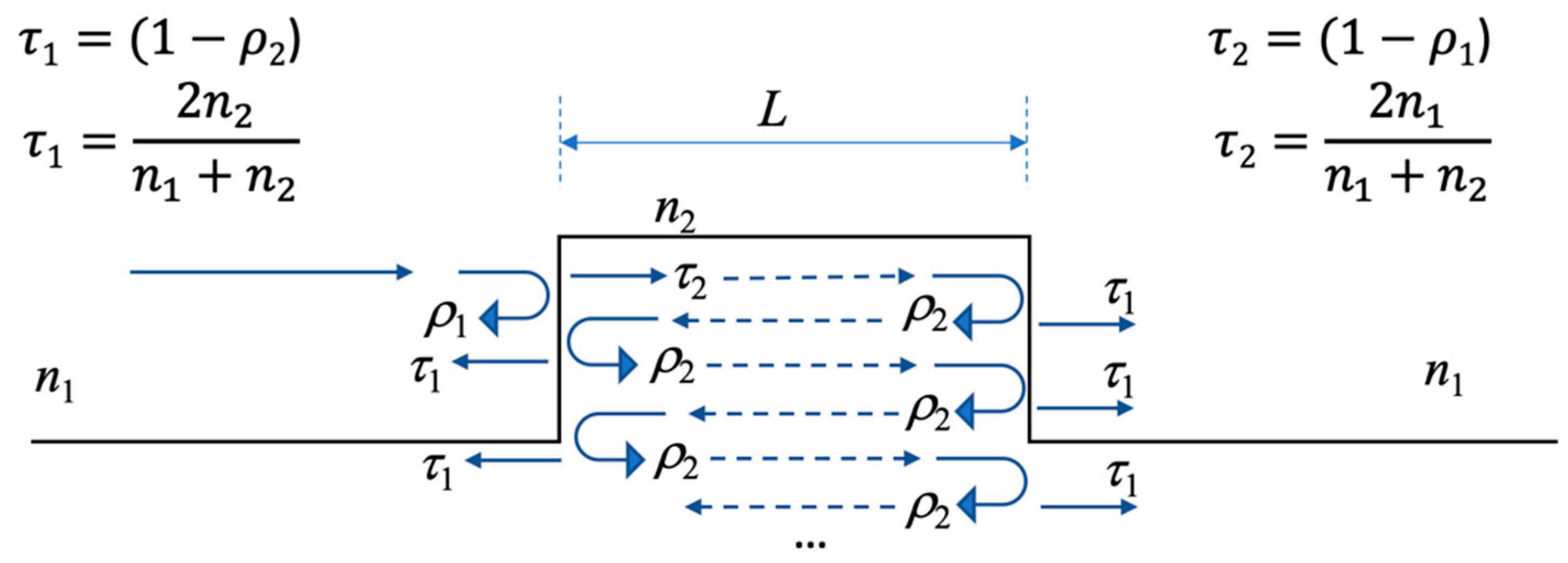
Then r_S is calculated by the sum of all the transmitted reflections:

\begin{matrix} ρ_{Σ} \equiv ρ_{1} + τ_{2} e^{i 2 k_{2} L} ρ_{2} τ_{1} + τ_{2} e^{i 4 k_{2} L} ρ_{2}^{3} τ_{1} + τ_{2} e^{i 6 k_{2} L} ρ_{2}^{5} τ_{1} + τ_{2} e^{i 8 k_{2} L} ρ_{2}^{7} τ_{1} + \dots (B .1) \end{matrix}

and since

ρ_{1} = - ρ_{2}

(see Figure 1):

\begin{matrix} ρ_{Σ} \equiv ρ_{1} + τ_{2} τ_{1} e^{i 2 k_{2} L} ρ_{2} - τ_{2} τ_{1} e^{i 4 k_{2} L} ρ_{2}^{2} ρ_{1} + τ_{2} τ_{1} e^{i 6 k_{2} L} ρ_{2}^{3} ρ_{1}^{2} - τ_{2} τ_{1} e^{i 8 k_{2} L} ρ_{2}^{4} ρ_{1}^{3} + \dots (B .2) \end{matrix}

also:

\begin{matrix} τ_{1} τ_{2} = (1 - ρ_{2}) (1 - ρ_{1}) = (1 + ρ_{1}) (1 - ρ_{1}) = (1 - ρ_{1}^{2}) (B .3) \end{matrix}

and therefore:

\begin{matrix} ρ_{Σ} \equiv ρ_{1} + (1 - ρ_{1}^{2}) e^{i 2 k_{2} L} ρ_{2} - (1 - ρ_{1}^{2}) e^{i 4 k_{2} L} ρ_{2}^{2} ρ_{1} + (1 - ρ_{1}^{2}) e^{i 6 k_{2} L} ρ_{2}^{3} ρ_{1}^{2} - (1 - ρ_{1}^{2}) e^{i 8 k_{2} L} ρ_{2}^{4} ρ_{1}^{3} + \dots (B .4) \end{matrix}

\begin{matrix} = (ρ_{1} + ρ_{2} e^{i 2 k_{2} L}) (1 - ρ_{1} ρ_{2} e^{i 2 k_{2} L} + ρ_{1}^{2} ρ_{2}^{2} e^{i 4 k_{2} L} - ρ_{1}^{3} ρ_{2}^{3} e^{i 46 L} + \dots) (B .5) \end{matrix}

But the expression in the second set of brackets on the RHS of Eq.B.5 is recognised to be an infinite geometric sum of the term

- ρ_{1} ρ_{2} e^{i 2 k_{2} L}

, hence:

\begin{matrix} ρ_{Σ} \equiv \frac{ρ_{1} + ρ_{2} e^{i 2 k_{2} L}}{1 - (- ρ_{1} ρ_{2} e^{i 2 k_{2} L})} = \frac{ρ_{1} + ρ_{2} e^{i 2 k_{2} L}}{1 + ρ_{1} ρ_{2} e^{i 2 k_{2} L}} (B .6) \end{matrix}

which is the hyperbolic sum rule of Eq.35 as required.

Appendix C. The HSR for a Graded Index (GRIN) and Absorptive Cavity

We model a graded index (GRIN) device (Figure C.1) to show explicitly that the hyperbolic sum rule (HSR) applies in more general circumstances (although here we have chosen parameters for analytical convenience).

For our notation of the complex refractive index n₂ we adopt the common convention (for example, Feynman [50] does this in Vol.1 §31-4) of a single prime indicating the real part

n_{2}^{'}

, and the double prime indicating the imaginary part

n_{2}^{''}

of the overall refractive index. Also, we define the refractive index to increase by a factor 1/α after each bounce, such that the overall refractive index for inside the etalon is given by:

\begin{matrix} n_{2} = \frac{n_{2}^{'}}{α^{m}} + i \frac{n_{2}^{''}}{α^{m}} (C .1) \end{matrix}

assuming the same functional form for the refractive n₁ outside of the etalon.

Figure C1. etalon featuring an absorptive medium n₂ and a sloped perfectly reflecting mirror.

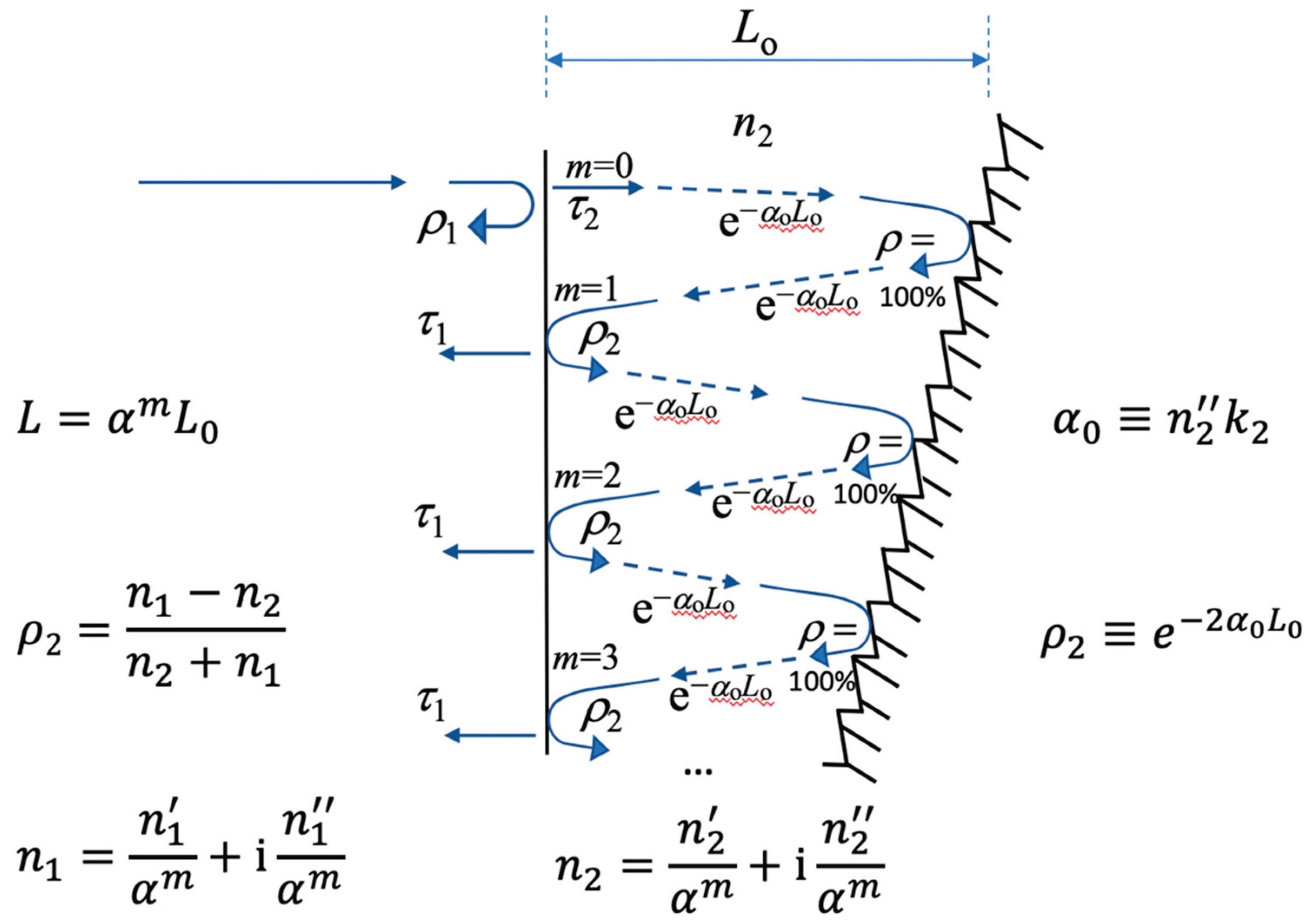
We note the free-space wavenumber k₀=2p/l, (such that k₂=n₂k₀) so that the additional (complex) phase accumulated by the wave on its m^th bounce (where the reduced cavity width is given by L=a^mL₀) is given by:

\begin{matrix} 2 k_{2} L = 2 n_{2} k_{0} L = 2 (\frac{n_{2}^{'}}{α^{m}} + i \frac{n_{2}^{''}}{α^{m}}) k_{0} α^{m} L_{0} = 2 (n_{2}^{'} + i n_{2}^{''}) k_{0} L_{0} (C .2) \end{matrix}

For the m^th bounce, the m^th transmitted reflection is then given by

\begin{matrix} τ_{2} {(e^{i 2 k_{2} L} ρ)}^{m} ρ_{2}^{m - 1} τ_{1} (C .3) \end{matrix}

Given r=1 (as per the perfect mirror on the RHS of the etalon of Fig.C.1) and noting that the absorption coefficient is given by

α_{0} \equiv n_{2}^{''} k_{0}

then Eq.C.3 can be simplified thus:

\begin{matrix} τ_{2} τ_{1} e^{i 2 n_{2}^{'} k_{0} L_{0} m} e^{- 2 n_{2}^{''} k_{0} L_{0} m} ρ_{2}^{m - 1} = (1 - ρ_{2}^{2}) e^{i 2 n_{2}^{'} k_{0} L_{0} m} e^{- 2 m α_{0} L_{0}} ρ_{2}^{m - 1} (C .4) \end{matrix}

We note that the Fresnel reflection and transmission coefficients maintain their same definitions as before, such that

τ_{1} τ_{2} = 1 - ρ_{2}^{2}

. We also design the absorption coefficient a₀ to be matched to the Fresnel reflection r₂ value such that:

\begin{matrix} ρ_{2} \equiv e^{- 2 α_{0} L_{0}} (C .5) \end{matrix}

and then the m^th transmitted wave out of the etalon allows simplification of Eq.C.4:

\begin{matrix} (1 - ρ_{2}^{2}) e^{i 2 n_{2}^{'} k_{0} L_{0} m} ρ_{2}^{m} ρ_{2}^{m - 1} = (1 - ρ_{2}^{2}) e^{i 2 n_{2}^{'} k_{0} L_{0} m} ρ_{2}^{2 m - 1} (C .6) \end{matrix}

giving (summing all the transmitted reflections and the initial reflection):

\begin{matrix} ρ_{Σ} \equiv ρ_{1} + (1 - ρ_{2}^{2}) e^{i 2 n_{2}^{'} k_{0} L_{0}} ρ_{2} + (1 - ρ_{2}^{2}) e^{i 4 n_{2}^{'} k_{0} L_{0}} ρ_{2}^{3} + (1 - ρ_{2}^{2}) e^{i 6 n_{2}^{'} k_{0} L_{0}} ρ_{2}^{5} + (1 - ρ_{2}^{2}) e^{i 8 n_{2}^{'} k_{0} L_{0} n} ρ_{2}^{7} τ_{1} + \dots (C .7) \end{matrix}

which is identical to Eq.B.4, so that:

\begin{matrix} ρ_{Σ} \equiv \frac{ρ_{1} + ρ_{2} e^{i 2 n_{2}^{'} k_{0} L_{0}}}{1 + ρ_{1} ρ_{2} e^{i 2 n_{2}^{'} k_{0} L_{0}}} (C .8) \end{matrix}

which is the HSR, as for the simple etalon previously discussed. However, we have now made the dissipation of the optical structure explicit via an absorption coefficient a₀ within the device.

We can also re-express Eq.C.8 as a temporal measure, by identifying wt ≡ k₀L₀ (making the initial width L₀ of the cavity essentially variable: that is, a proxy for the spatial x-axis) so we have:

\begin{matrix} ρ_{Σ} (t) = \frac{ρ_{1} + ρ_{2} e^{i 2 n_{2}^{'} ω t}}{1 + ρ_{1} ρ_{2} e^{i 2 n_{2}^{'} ω t}} (C .9) \end{matrix}

Appendix D. Hilbert Transform of HSR Function for an Etalon

The Hilbert transform relies on the mathematical properties of analytic functions in the complex plane such that two functions which form a Hilbert transform pair can be combined as the real and imaginary parts of an analytic function in the complex plane. It is instructive to re-express the Eq.35 as a temporal measure. In particular, invoking w/k=c and making the width L of the cavity essentially variable (i.e. a proxy for the spatial x-axis) we explicitly invoke a real time t and rewrite Eq.35 as:

\begin{matrix} ρ_{Σ} (t) = \frac{ρ_{1} + ρ_{2} e^{i 2 n_{2} ω t}}{1 + ρ_{1} ρ_{2} e^{i 2 n_{2} ω t}} (D .1) \end{matrix}

For simplicity of notation we take advantage of the relation r₁=−r₂ ≡ r to write:

\begin{matrix} ρ_{Σ} (t) = \frac{ρ (1 - e^{i 2 n_{2} ω t})}{1 - ρ^{2} e^{i 2 n_{2} ω t}} (D .2) \end{matrix}

The real and imaginary parts of Eq.D.2 can be shown to be:

\begin{matrix} ρ_{Σ} {(t)}_{Re} = \frac{(1 + ρ^{2}) (1 - \cos 2 n_{2} ω t)}{1 - 2 ρ^{2} \cos 2 n_{2} ω t + ρ^{4}} (D .3 a) \end{matrix}

and

\begin{matrix} ρ_{Σ} {(t)}_{Im} = \frac{(ρ^{2} - 1) \sin 2 n_{2} ω t}{1 - 2 ρ^{2} \cos 2 n_{2} ω t + ρ^{4}} (D .3 b) \end{matrix}

The interesting thing to note is that the Eqs.D.3 representing the real and imaginary parts of the temporal response r_S(t) are Hilbert transforms of each other. This Hilbert transform relationship can be demonstrated as follows, by referring to Eq.B.4, and substituting again for k₂L with wt, as well as for r₁=−r₂ ≡ r :

The real part of r_S(t) is then simply seen by inspection (using the Euler identity) to be:

\begin{matrix} ρ_{Σ} {(t)}_{Re} = \frac{(1 - ρ^{2})}{ρ} [\frac{ρ^{2}}{(1 - ρ^{2})} - \sum_{m = 1}^{\infty} {(- ρ^{2})}^{m} \cos 2 m n_{2} ω t] (D .5 a) \end{matrix}

And the imaginary part is

\begin{matrix} ρ_{Σ} {(t)}_{Im} = - \frac{(1 - ρ^{2})}{ρ} \sum_{m = 1}^{\infty} {(- ρ^{2})}^{m} \sin 2 m n_{2} ω t (D .5 b) \end{matrix}

Ignoring the d.c. term in Eq.D.5a (independent of time t) we can see that on a term-by-term basis, the quantities

\cos 2 m n_{2} ω t

and

\sin 2 m n_{2} ω t

are Hilbert transforms of each other.

In addition, analytically continuing Eq.D.1 into the complex temporal z-plane, given by z=t+it, we can also show how the Etalon HSR function is also essentially analytic (holomorphic) and obeys the Cauchy-Riemann equations:

\begin{matrix} ρ_{Σ} (t, τ) = \frac{ρ_{1} + ρ_{2} e^{i 2 n_{2} ω (t + i τ)}}{1 + ρ_{1} ρ_{2} e^{i 2 n_{2} ω (t + i τ)}} (D .6) \end{matrix}

Using

ρ_{1} = - ρ_{2}

≡ r we have:

\begin{matrix} ρ_{Σ} (t, τ) = ρ \frac{1 - e^{i 2 n_{2} ω t} e^{- 2 n_{2} ω τ}}{1 - ρ^{2} e^{i 2 n_{2} ω t} e^{- 2 n_{2} ω τ}} (D .7) \end{matrix}

Then the real and imaginary components are:

\begin{matrix} ρ_{Σ} {(t, τ)}_{Re} = ρ \frac{1 - (1 + ρ^{2}) e^{- 2 n_{2} ω τ} \cos 2 n_{2} ω t + ρ^{2} e^{- 4 n_{2} ω τ}}{1 - 2 ρ^{2} e^{- 2 n_{2} ω τ} \cos 2 n_{2} ω t + ρ^{4} e^{- 4 n_{2} ω τ}} (D .8 a) \end{matrix}

and

\begin{matrix} ρ_{Σ} {(t, τ)}_{Im} = ρ \frac{(ρ^{2} - 1) e^{- 2 n_{2} ω τ} \sin 2 n_{2} ω t}{1 - 2 ρ^{2} e^{- 2 n_{2} ω τ} \cos 2 n_{2} ω t + ρ^{4} e^{- 4 n_{2} ω τ}} (D .8 b) \end{matrix}

We confirm that these real and imaginary components obey the Cauchy-Riemann equations for analyticity in the complex temporal z-plane:

\begin{matrix} \frac{\partial ρ_{Σ} {(t, τ)}_{Re}}{\partial t} = \frac{\partial ρ_{Σ} {(t, τ)}_{Im}}{\partial τ} and \frac{\partial ρ_{Σ} {(t, τ)}_{Re}}{\partial τ} = - \frac{\partial ρ_{Σ} {(t, τ)}_{Im}}{\partial t} (D .9) \end{matrix}

Taking each of the terms in turn:

\begin{matrix} \frac{\partial ρ_{Σ} {(t, τ)}_{Re}}{\partial t} = 2 n_{2} ω ρ e^{- 2 n_{2} ω τ} (1 - ρ^{2}) \sin 2 n_{2} ω t \frac{(1 - ρ^{4} e^{- 4 n_{2} ω τ})}{{(1 - 2 ρ^{2} e^{- 2 n_{2} ω τ} \cos 2 n_{2} ω t + ρ^{4} e^{- 4 n_{2} ω τ})}^{2}} (D .10 a) \end{matrix}

\begin{matrix} \frac{\partial ρ_{Σ} {(t, τ)}_{Re}}{\partial τ} = 2 n_{2} ω ρ e^{- 2 n_{2} ω τ} (1 - ρ^{2}) \frac{(1 + ρ^{4} e^{- 4 n_{2} ω τ}) \cos 2 n_{2} ω t - 2 ρ^{2} e^{- 2 n_{2} ω τ}}{{(1 - 2 ρ^{2} e^{- 2 n_{2} ω τ} \cos 2 n_{2} ω t + ρ^{4} e^{- 4 n_{2} ω τ})}^{2}} (D .10 b) \end{matrix}

And likewise,

\begin{matrix} \frac{\partial ρ_{Σ} {(t, τ)}_{Im}}{\partial t} = - 2 n_{2} ω ρ e^{- 2 n_{2} ω τ} (1 - ρ^{2}) \frac{(1 + ρ^{4} e^{- 4 n_{2} ω τ}) \cos 2 n_{2} ω t - 2 ρ^{2} e^{- 2 n_{2} ω τ}}{{(1 - 2 ρ^{2} e^{- 2 n_{2} ω τ} \cos 2 n_{2} ω t + ρ^{4} e^{- 4 n_{2} ω τ})}^{2}} (D .11 a) \end{matrix}

\begin{matrix} \frac{\partial ρ_{Σ} {(t, τ)}_{Im}}{\partial τ} = 2 n_{2} ω ρ e^{- 2 n_{2} ω τ} (1 - ρ^{2}) \sin 2 n_{2} ω t \frac{(1 - ρ^{4} e^{- 4 n_{2} ω τ})}{{(1 - 2 ρ^{2} e^{- 2 n_{2} ω τ} \cos 2 n_{2} ω t + ρ^{4} e^{- 4 n_{2} ω τ})}^{2}} (D .11 b) \end{matrix}

References

Parker, M.C.; Jeynes, C. Relating a system’s Hamiltonian to its Entropy Production using a Complex-Time approach. Entropy 2023, 25 629. [Google Scholar] [CrossRef] [PubMed]
John S. Toll, Causality and the Dispersion Relation: Logical Foundations. Phys. Rev. 1956, 104, 1760–1770. [Google Scholar] [CrossRef]
Tour, James M.; Parker, M. C.; Jeynes, C. Thermodynamic Limitations on the Natural Emergence of Long Chain Molecules: Implications for Origin of Life. BioCosmos 2025, 5, 64–71. [Google Scholar] [CrossRef]
Parker, Michael C.; Walker, Stuart D. A Unified Carnot Thermodynamic and Shannon Channel Capacity Information-Theoretic Energy Efficiency Analysis. IEEE Trans. Commun. 2014, 62, 3552–3559. [Google Scholar] [CrossRef]
Parker, Michael C.; Jeynes, Chris; Walker, Stuart D. A Metric for the Entropic Purpose of a System. Entropy 2025, 27 131, 40pp. [Google Scholar] [CrossRef] [PubMed]
George F. R. Ellis, Efficient, Formal, Material, and Final Causes in Biology and Technology. Entropy 2023, 25 1301. [CrossRef] [PubMed]
Parker, M.C.; Walker, S.D. A dynamic model of information and entropy. Entropy 2010, 12, 80–88. [Google Scholar] [CrossRef]
Parker, M.C.; Jeynes, C. Maximum Entropy (Most Likely) Double Helical and Double Logarithmic Spiral Trajectories in Space-Time. Sci. Rep. 10779 (10 pp, 44 pp Appendices). 2019, 9. [Google Scholar] [CrossRef] [PubMed]
Stenner, Michael D.; Gauthier, Daniel J.; Neifeld, Mark A. Fast Causal Information Transmission in a Medium With a Slow Group Velocity. Phys. Rev. Lett. 2005, 94, 053902. [Google Scholar] [CrossRef] [PubMed]
Parker, M.C.; Jeynes, C. Entropic Uncertainty Principle, Partition Function and Holographic Principle derived from Liouville's Theorem. Phys. Open 2021, 7, 100068. [Google Scholar] [CrossRef]
Eugene P. Wigner, On the Development of the Compound Nucleus Model. Am. J. Phys. 1955, 23, 371–380. [CrossRef]
Abriola; Dimitriou, P. Development of a Reference Database for Ion Beam Analysis", Report of a Coordinated Research Project (CRP) on Reference Database for Ion Beam Analysis (IAEA-TECDOC-1780). IAEA, Vienna, 2015; Available online: http://www-pub.iaea.org/MTCD/Publications/PDF/TE-1780_web.pdf.
Parker, M.C.; Jeynes, C.; Walker, S.D. A hyperbolic sum rule for probability: solving recursive (“Chicken & Egg”) problems. Entropy 2025, 27 352, 40pp. [Google Scholar] [CrossRef] [PubMed]
Karl Weierstrass, "Über continuirliche Functionen eines reellen Arguments, die für keinen Werth des letzeren einen bestimmten Differentialquotienten besitzen". In this paper was read in 1872 to the (Berlin) Prussian Academy of Science Mathematische Werke von Karl Weierstrass; Berlin: Mayer & Mueller, 1895; Vol. 2.
Mary Rees, One hundred years of complex dynamics. Proc. R. Soc. A Math. Phys. Eng. Sci. 2016, 472 2185. [CrossRef] [PubMed]
Cox, R.T. Probability, frequency and reasonable expectation. Am. J. Phys. 1946, 14, 1–13. [Google Scholar] [CrossRef]
Jaynes, E.T. On the Rationale of Maximum Entropy Methods. Proc. IEEE 1982, 70, 939–952. [Google Scholar] [CrossRef]
Terrence Deacon, Incomplete Nature: How Mind Emerged from Matter; New York, 2011; Available online: W.W.Norton.
Cerisier, P.; Porterie, B.; Kaiss, A.; Cordonnier, J. Transport and sedimentation of solid particles in Bénard hexagonal cells. Eur. Phys. J. E 2005, 18, 85–93. [Google Scholar] [CrossRef] [PubMed]
Grecian, W. James; Lane, Jude V.; Michelot, Théo; Wade, Helen M.; Hamer, Keith C. Understanding the ontogeny of foraging behaviour: Insights from combining marine predator bio-logging with satellite-derived oceanography in hidden Markov models. J. R. Soc. Interface 2018, 15, 20180084. [Google Scholar] [CrossRef] [PubMed]
Prants, Sergey V. Marine life at Lagrangian fronts. Prog. Oceanogr. 2022, 204, 102790. [Google Scholar] [CrossRef]
Prigogine, Ilya. Time, Structure, and Fluctuations. Science 1978, 201, 777–785. [Google Scholar] [CrossRef] [PubMed]
Gobato, Ricardo; Mitra, Abhijit; Mullick, Poulomi. Extratropical cyclone in the South Georgia and south sandwich islands and double spiral galaxies. Phys. Astron. Int. J. 2023, 7, 157–161. [Google Scholar] [CrossRef]
Landauer, Rolf. Information is a physical entity. Physica A Stat. Mech. Its Appl. 1999, 263, 63–67. [Google Scholar] [CrossRef]
Shannon, C. E. Communication in the presence of noise. Proc. Inst. Radio Eng. 37(1949), 10–21. [CrossRef]
Essiambre, René-Jean; Kramer, Gerhard; Winzer, Peter J.; Foschini, Gerard J.; Goebel, Bernhard. Capacity Limits of Optical Fiber Networks. J. Light Wave Technol. 2010, 28, 662–701. [Google Scholar] [CrossRef]
Agrawal, Govind P. Optical Communication: Its History and Recent Progress (Ch.8. In Optics in Our Time; Al-Amri, M.D., et al., Eds.; Springer, 2016. [Google Scholar] [CrossRef]
Pietro Redondi, Galileo Eretico. In Raymond Rosenthal, Galileo: Heretic; Giulio Einaudi: Turin; Princeton University Press, 1983.
Ferrone, Vincenzo; Firpo, Massimo. From Inquisitors to Microhistorians: A Critique of Pietro Redondi's Galileo eretico. J. Mod. Hist. 1986, 58, 485–524. Available online: (https://www.jstor.org/stable/1879919 ). [CrossRef]
Thijssen, Hans. Condemnation of 1277. In Stanford Encyclopedia of Philosophy, 2003; Winter 2023 Edition; accessed; Zalta, Edward N., Nodelman, Uri, Eds.; (accessed on 18/8/2026).
Alexandre Koyré, “Le vide et l’espace infini au XIVe siècle,” Etudes de l’histoire de la pensée philosophique; originally published in 1949; Gallimard: Paris, 1961.
Hans Küng, Great Christian Thinkers; Continuum Books: New York, 1994.
Jeynes, C. (Ed.) Stanley Jaki, Science and Creation, from eternal cycles to an oscillating universe; Scottish Academic Press: Edinburgh, 1974; Available online: https://www.surrey.ac.uk/sites/default/files/2021-03/science-and-creation.pdf (accessed on 18/8/2023).
Moody, Ernest Addison (Ed.) John Buridan (ca.1295-ca.1358), Quaestiones super quattuor libris de caelo et mundo; The Medieval Academy of America: Cambridge Mass., 1942. [Google Scholar]
E.A. Moody in Dictionary of Scientific Biography; Scribners: New York, 1970.
Marshall Clagett, The Science of Mechanics in the Middle Ages; University of Wisconsin Press: Madison, 1959.
Stillman Drake, Galileo's Discovery of the Law of Free Fall. Sci. Am. 1973, 228, 84–93. Available online: https://www.jstor.org/stable/10.2307/24923051. [CrossRef]
Edward Grant, Physical Science in the Middle Ages; Cambridge University Press, 1971.
Stillman Drake, Impetus Theory Reappraised. J. Hist. Ideas 1975, 36, 27–46. Available online: http://www.jstor.com/stable/2709009.
Mueller, Ian. Homogeneity in Eudoxus's Theory of Proportion. Arch. Hist. Exact. Sci. 1970, 7, 1-6. Available online: https://www.jstor.org/stable/41133314. [CrossRef]
Stillman Drake, A Further Reappraisal of Impetus Theory: Buridan, Benedetti and Galileo. Stud. Hist. Philos. Sci. 1976, 7, 319–336. [CrossRef]
J.M. Keynes, Newton the Man (Ch.35 in: Essays in Biography; Palgrave Macmillan: London, 2010; pp. 363–374. [CrossRef]
John Lee Longeway, Demonstration and Scientific Knowledge in William of Ockham; University of Notre Dame Press, 2007.
Kedar, Yael; Hon, Giora. Natures’ and ‘Laws’: The making of the concept of law of nature - Robert Grosseteste (c.1168-1253) and Roger Bacon (1214/1220-1292). Stud. Hist. Philos. Sci. Part A 2017, 61, 21–31. [Google Scholar] [CrossRef] [PubMed]
Alistair C. Crombie, Robert Grosseteste and the origins of experimental science; Oxford University Press, 1953.
Belkind, Ori. Unnatural acts: The transition from Natural Principles to Laws of Nature in Early Modern science. Stud. Hist. Philos. Sci. Part A 2020, 81, 62–73. [Google Scholar] [CrossRef] [PubMed]
Paul Forman, Weimar Culture, Causality, and Quantum Theory, 1918-1927: Adaptation by German Physicists and Mathematicians to a Hostile Intellectual Environment. Hist. Stud. Phys. Sci. 1971, 3, 1–115. Available online: https://www.jstor.org/stable/2775731. [CrossRef]
Vane-Wright, Richard I.; Corning, Peter A. Teleonomy in living systems. Biol. J. Linn. Soc. 2023, 139, 341–356. [Google Scholar] [CrossRef]
Corning, Peter A.; Kauffman, S. A.; Noble, Denis; Shapiro, J. A.; Vane-Wright, R. I. Evolution “On Purpose” Teleonomy in Living Systems; MIT Press: Cambridge, MA, 2023. [Google Scholar] [CrossRef]
Richard Feynman, Robert B. Leighton, Matthew Sands, The Feynman Lectures on Physics; Addison-Wesley: Reading, MA, 1965.

Figure 1. Optical cavity with refractive index n₂ in a medium of refractive index n₁.

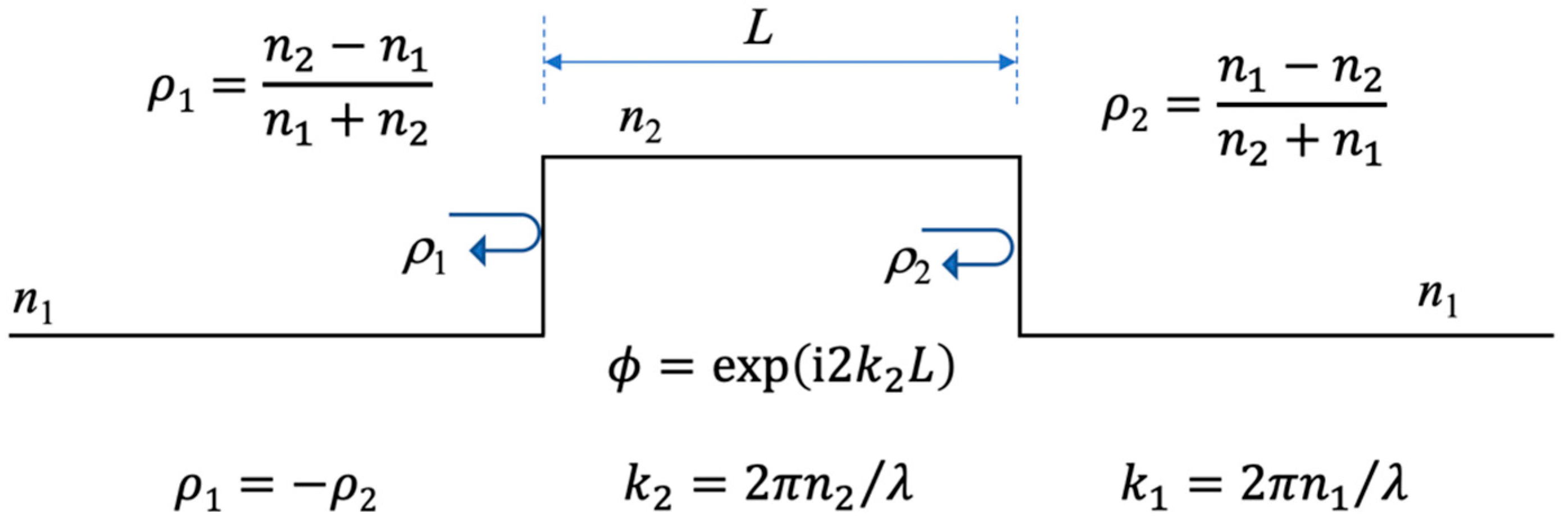
Figure 2. Funnel-like (circular) absorptive optical waveguide etalon: a) Single light trajectory (traveling whispering gallery mode) along device; (b) Plan view of logarithmic spiral trajectory; (c) Plan view of two logarithmic spiral trajectories entering at different locations; (d) Double logarithmic spiral (DLS) trajectory, side view.

Disclaimer/Publisher’s Note: The statements, opinions and data contained in all publications are solely those of the individual author(s) and contributor(s) and not of MDPI and/or the editor(s). MDPI and/or the editor(s) disclaim responsibility for any injury to people or property resulting from any ideas, methods, instructions or products referred to in the content.

© 2026 by the authors. Licensee MDPI, Basel, Switzerland. This article is an open access article distributed under the terms and conditions of the Creative Commons Attribution (CC BY) license (http://creativecommons.org/licenses/by/4.0/).

Copyright: This open access article is published under a Creative Commons CC BY 4.0 license, which permit the free download, distribution, and reuse, provided that the author and preprint are cited in any reuse.