

Submitted:
11 September 2026
Posted:
15 September 2026
You are already at the latest version
Abstract
We investigate whether gravity-like dynamics can emerge from transformations of finite relational records rather than from matter evolving in a pre-existing spacetime. In Dendrographic Holographic Theory (DHT), finite ordered dendrograms define exact relational states, causal growth trajectories, and representation-specific probability distributions. We analyzed Path, Embedding, Views, and Branch-Monna entropies in incoming and forward ensembles. Their terminal-referenced entropy variables were well described by Newtonian inverse-square and Schwarzschild-like radial profiles, with broad but non-universal held-out predictive support and an overall predictive advantage for the Schwarzschild-like form. Independent four-dimensional reconstructions produced Lorentzian target-local geometries whose Einstein tensors showed robust held-out proportionality to entropy-derived source tensors, revealing a recurring trajectory-local GR-like organization without establishing the Einstein equations of physical spacetime. We then formulate a trajectory-supported differential completion in exact Z = (τ,ϕ) coordinates. Exact induced transitions are timelike under an explicit flat anchored reference metric. Representation-specific probability laws remain defined only on supported exact DHT states or ordered state pairs, whose finite Shannon entropies provide exact anchors for smooth auxiliary two-endpoint scalar fields. Level-balanced relational derivatives define a premetric informational tensor and an action-derived source tensor. Under a single-effective-gradient reduction, this source reduces to the kinetic entropy source used in the numerical tensor reconstruction, providing an explicit connection between the empirical and theoretical constructions. An auxiliary local metric action of Einstein--Hilbert form defines an Einstein-like Euler--Lagrange tensor. Within this chosen geometrical construction, a constructive curvature-jet argument establishes nonempty anchored metric segments on the elementary regular transition domain, with \( G_{\mu\nu}
=
\kappa_qT_{\mu\nu}^{(q)} \) holding along the corresponding DHT trajectories. This construction does not constitute a derivation of the Einstein field equations from DHT. Generic continuum points supply only the transverse differential data required for curvature and are not additional DHT states. The Views and Branch-Monna sectors retain their exact quantum-like state and event-level interpretations without introducing probability laws on non-exact continuum points.
Keywords:
entropic-gravity-like
; relational information
; dendrograms
; trees
; p-adic string sets
1. Introduction
The relation between gravitation, thermodynamics, and information suggests that gravitational behaviour may not be fundamental in the conventional sense, but may instead emerge from the statistical organization of underlying degrees of freedom. In thermodynamic approaches to gravity, the Einstein field equations can be related to horizon thermodynamics, while in entropic-gravity constructions an effective force arises from the entropy change associated with the displacement of a system relative to an information-bearing boundary or source [1,2]. These approaches motivate the possibility that gravitational laws may describe collective informational organization rather than only interactions imposed on pre-existing material objects in a fixed spacetime.
Related questions arise in background-independent and relational approaches to gravity, including shape dynamics, loop quantum gravity, spin-foam models, and causal-set theory [3,4,5,6,7]. Although these programs differ substantially in their assumptions and mathematical structures, they share an attempt to formulate geometry without taking a fixed external spacetime as the only possible starting point. Machian ideas have likewise motivated theories in which the physical properties of a system are defined, at least partly, through its relations to other systems rather than through an independently specified background [8].
A complementary mathematical tradition has explored non-Archimedean and ultrametric structures in physics. p-adic analysis has been applied to mathematical physics, string amplitudes, cosmology, quantum models, and number-theoretic formulations of fundamental dynamics [9,10,11,12,13,14]. More recently, p-adic conformal field theories, tensor networks, and p-adic AdS/CFT constructions have used hierarchical trees and non-Archimedean boundary structures to study holography and emergent geometry [15,16,17,18,19]. Ultrametric organization also plays a central role in the hierarchical state spaces of spin-glass and disordered-system models [20,21].
These theories do not constitute one common physical model. Some introduce p-adic numbers directly into amplitudes or dynamical laws, some use Bruhat-Tits-like trees as holographic geometries, and others encounter ultrametricity through the hierarchical organization of states. Their common importance for the present work is more limited but fundamental: they demonstrate that tree structures, ultrametric distances, and non-Archimedean organization can provide mathematically meaningful state spaces for physical theories.
Dendrographic Holographic Theory (DHT) uses these mathematical structures in a different way. It does not posit a p-adic physical spacetime, a p-adic string amplitude, or a p-adic conformal field theory. Instead, finite ordered dendrograms represent the relational information available to an observer. Their p-adic branch encodings and induced ultrametric relations describe how acquired events are organized relative to one another. The resulting relational records are subsequently mapped into real coordinate and probability-distribution spaces in which geometric and dynamical questions can be formulated.
This leads to the specific problem addressed here. Can gravity-like force laws and geometric dynamics arise in a system whose primitive states are not particles moving through a pre-existing physical spacetime, but finite relational structures and their admissible transformations? Addressing this question requires more than observing a correlation between entropy and an arbitrarily chosen distance. The relational states, probability spaces, entropy variables, coordinate representations, and geometrical quantities must all be explicitly distinguished.
DHT provides a setting in which these requirements can be investigated. It is a relational-information framework developed through a series of analytical and numerical studies [22,23,24,25,26,27,28,29]. An observer’s distinctions organize finite events into ordered rooted dendrograms. These dendrograms are not treated as objects already located within a physical spacetime. They are finite records of the relational organization available to the observer at a given stage of measurement.
The framework is grounded in a Leibniz-Mach principle of relational identity: physical distinctions are defined through relationally accessible properties, and states that cannot be distinguished within the available relational description are identified at that level [30,31].
The detailed DHT construction is not repeated in this Introduction. Its relational identity principle, ordered p-adic dendrograms, Monna map, induced relational configurations, four-coordinate representations, growth-based causal order, Views distributions, information geometry, and previous quantum-like results are reviewed in Appendix I. The probability spaces and entropy definitions used in the present numerical analysis are introduced in Section 2.2 and detailed in Appendix B.
1.1. Complete and Reduced DHT Relational State Spaces
The present study builds on two previously developed DHT state spaces. The first represents complete finite dendrogramic states. Within the admissible class used here, each exact dendrogram T has a lossless four-dimensional real representation,
The unhatted coordinate represents the complete dendrogramic relational state rather than only a statistical summary of that state.
Admissible event insertion generates trajectories through this coordinate space. Each insertion adds an event while preserving the internal relations already contained in the previous dendrogram. Exact induced containment of an earlier dendrogram in a later dendrogram therefore defines a growth-based causal relation. Dendrograms connected by such growth-preserving containment are timelike related in the exact DHT sense, whereas dendrograms for which no such containment relation exists are DHT-spacelike, or induced-incomparable.
These terms refer to the exact growth-based causal classification. For the fundamental Lorentzian metric developed below, every strict induced successor has a displacement inside the corresponding future timelike cone, but the converse is not imposed. Exact induced-incomparability therefore need not imply spacelike separation under the fundamental Lorentzian metric.
The resulting organization is Minkowski-like because it distinguishes relational past, future, and non-containment sectors within a four-dimensional real representation. This terminology refers to the causal organization of the relational state space. It does not imply that the unhatted coordinate space has already been identified with measured physical spacetime.
The second state space is constructed from the pairwise relational separations encoded by a dendrogram. Finite 2-adic branch codes are mapped through the Monna map to rational values on , and their pairwise absolute differences define the dendrogram’s Views. The normalized multiplicities of the resulting values form the Views distribution .
Within the admissible DHT family, the complete Views distribution has a separate lossless four-dimensional representation,
The hatted and unhatted coordinates therefore represent different objects. The unhatted coordinate represents the complete dendrogramic state, whereas the hatted coordinate represents its reduced Views distribution.
The map from dendrogram structure to the Views distribution is generally many-to-one. Distinct complete dendrograms may generate the same pairwise Views distribution. By contrast, within the restricted family of DHT-generated distributions, provides a lossless parametrization of the complete distribution. The relevant structure is therefore
The non-injectivity occurs in the projection , not in the representation of an admissible Views distribution by .
This distinction is essential for the present analysis. The radial and tensor constructions are defined on the unhatted dendrogramic coordinate space because that space retains the complete relational state, its position along a dendrogramic trajectory, and its growth-based causal relations. The hatted space enters later when the Views-sector geometry is connected to the previous DHT quantum-like construction.
Earlier DHT studies used the Views distribution to define a complex representative whose modulus is determined by , and developed associated phase, Hamilton-Jacobi, continuity, Fisher-information, and Bohmian-like quantum-potential structures [26,27,28]. The present work does not rederive those results. It asks whether transformations of the complete dendrogramic states additionally exhibit gravity-like radial relations and a GR-like relation between informational dynamics and relational geometry.
1.2. Informational Descriptions and Directional Ensembles
A dendrogramic transformation can be examined through several distinct probability spaces. The present study uses four complementary informational representations: Path, Embedding, Views, and Branch-Monna. They retain information about different aspects of the same relational transformation, including its history, its realization within a terminal host, its pairwise organization, and the incorporation of a newly acquired event.
These representations are not assumed to provide interchangeable estimates of one underlying entropy. Each defines its own weighted count space, probability distribution, entropy, terminal reference, and sign convention. Their simultaneous use tests whether gravity-like behaviour is restricted to one specially chosen informational construction or recurs across distinct descriptions of dendrogramic transformation. Their formal definitions are introduced in Section 2.2 and detailed in Appendix B.
The study also distinguishes incoming and forward transformation directions. The two sectors use the same event distribution and the same deterministic dendrogram-growth rule but impose different relational boundary conditions.
Forward ensembles are conditioned on selected initial dendrograms. Additional events are inserted sequentially, and the ensemble describes the possible relational histories developing from the common initial state. Incoming ensembles are conditioned on selected terminal dendrograms. They consist of ordinary forward-generated histories retained because they reach the specified terminal target.
Scope of the present study.
The present work investigates whether the informational changes generated by dendrogramic transformations exhibit gravity-like radial relations and a GR-like tensor closure in the pre-existing unhatted DHT relational-coordinate space. The numerical analyses and the subsequent continuum formulation are kept logically distinct: the former test finite target-conditioned trajectories, whereas the latter proposes an ambient relational framework in which those numerical observations may be interpreted.
1.3. Questions Addressed and Study Structure
The study addresses three successive questions:
- 1.
- Do terminal-referenced entropy differences generated by dendrogramic transformations follow Newtonian inverse-square and Schwarzschild-like informational force profiles, and do those profiles predict omitted relational levels?
- 2.
- Do registered target-conditioned trajectories support a four-dimensional Lorentzian reconstruction in which the trajectory-local Einstein tensor exhibits held-out proportionality to a source derived from the corresponding informational scalar?
- 3.
- Can the radial informational-force description, the numerical tensor closure, and the previous DHT quantum-like representations be situated within one anchored relational continuum framework without identifying the resulting geometry prematurely with physical spacetime?
The first question is examined across the Path, Embedding, Views, and Branch-Monna representations and in both incoming and forward transformation directions. The second is tested independently through target-local metric, derivative, curvature, source, and held-out closure reconstructions.
The numerical force-law and tensor results are presented before the general theoretical formulation. This ordering allows the theoretical construction to be motivated and constrained by the numerical behaviour without assuming the continuum field equation in advance.
The general theoretical section then develops an auxiliary differential completion of the exact dendrogramic states through anchored Lorentzian metric data, smooth scalar continuations of exact entropy anchors, and a trajectory-supported Einstein-like closure. The underlying representation-specific probability laws themselves remain confined to the supported exact DHT states or state pairs. The subsequent wavefunction sections examine how the Views and Branch-Monna representations connect the geometrical findings to state-level and event-level quantum-like descriptions. The Discussion compares the construction with thermodynamic and entropic gravity, distinguishes the numerical and continuum claims, and outlines the requirements for a future covariant coupled theory.
2. Numerical Methods
2.1. Generation of the Forward and Incoming Dendrogram Ensembles
2.1.1. Incremental Ultrametric Construction
Both directions used the same deterministic incremental ultrametric construction. Starting from , each new event was attached above the rooted clade minimizing the squared discrepancy between its Euclidean distances to the existing events and the candidate cophenetic ultrametric distances. The attachment height was restricted to the interval compatible with the existing hierarchy, with deterministic tie breaking.
Each insertion added one leaf while preserving all previous internal relations, so
Hence every generated sequence is a growth-preserving DHT trajectory. The complete insertion rule is given in Appendix A and Supplementary Software S1.
2.1.2. Initial- and Terminal-Conditioned Ensembles
The forward ensemble was conditioned on initial dendrograms at , with ten target topologies at each n, giving thirty targets. For target , additional realizations of the same initial topology were obtained from
Because the transformation is positive affine, it preserves the ordering and therefore the initial dendrogram topology.
Seven new events were then inserted sequentially, giving . For each initial target, histories were generated.
The incoming ensemble was conditioned instead on terminal dendrograms at . For each M, a pilot ensemble of independent standard-normal event sequences was used to select the ten most frequent terminal topologies. For each selected target , newly sampled histories were retained only when , until at least accepted histories were obtained.
Incoming histories remained ordinary forward-generated sequences ; only the final eight levels, , were analyzed. Thus incoming and forward ensembles used the same event distribution and insertion rule and differed only by terminal versus initial conditioning.
2.2. Representation-Specific Probability and Entropy Distributions
Each history was analyzed through four informational representations: Path, the retained history prefix; Embedding, one realized embedding of the current dendrogram into its corresponding terminal dendrogram; Views, the pooled distribution of pairwise Monna separations; and Branch-Monna, the Monna coordinate of the newly inserted branch.
For every target, direction, and level, representation-specific objects were pooled using their occurrence weights before normalization and entropy calculation. The resulting entropy was therefore the entropy of the complete weighted distribution, not an average of per-history or per-topology entropies.
All representations used the terminal level M as reference. For ,
Embedding retained the opposite orientation,
In both directions, Embedding was terminal-directed: every level-m dendrogram was embedded into its corresponding level-M dendrogram. Complete sample-space, pooling, and entropy definitions are given in Appendix B.
2.3. Registered Target-Level Coordinates and Relational Radial Coordinates
Each realized dendrogram has an exact four-dimensional coordinate . The registered coordinate of the target-conditioned ensemble at level ℓ was its occurrence-weighted barycentre,
For every representation q and direction d, the numerical coordinate was
Thus each numerical state represents an ensemble barycentre rather than one exact dendrogram. Embedding used this same coordinate; the terminal dendrogram entered its entropy construction but was not subtracted from .
Suppressing within one panel, write . Candidate three-coordinate radii were
giving . The radius was calculated after ensemble coordinate aggregation, not averaged over individual-state radii.
2.3.1. Panel-Wise Radial-Coordinate Selection
The four radii were evaluated separately in each representation-direction panel. Selection required balanced support for both Newtonian and Schwarzschild-like models across all three cohorts: candidates were ranked first by the weaker model in the worst-performing cohort and then by their remaining balanced performance.
One radius was selected per panel and then fixed for all targets, cohorts, direct fits, and leave-one-level-out folds in that panel. The exact lexicographic criterion is given in Appendix C.
2.4. Informational Force-Law Fitting and Validation
For target a, the signed entropy variable was interpreted as a target-normalized informational force,
where was taken constant across that target’s retained levels but was not independently estimated. Hence the fitted quantity is not an absolute physical force.
Cohort trajectories were obtained by averaging target radii and entropy variables at each relational level. Figure error bars show target-wise standard deviations; standard errors were also retained. Definitions are given in Appendix C.2.
2.4.1. Force-Law Models and Parameter Fitting
The fitted model families were
Both were fitted separately to cohort-level and individual-target trajectories. Parameter constraints required positive effective radii and a real Schwarzschild-like denominator over every fitted and evaluated observation. Full constraints and fitting details are given in Appendix C.3 and Supplementary Software S1.
2.4.2. Post-Selection Leave-One-Level-Out Validation
Because the Schwarzschild-like model has one additional shape parameter, the primary comparison was based on held-out prediction rather than direct-fit .
Leave-one-level-out validation was performed after panel-wise radius selection, with the selected radius held fixed in every fold. Thus validation was conditional on the selected coordinate and was not a nested validation of radius selection.
The procedure was applied separately to all cohort-level and individual-target trajectories. In each fold, one relational level was omitted, all force-law parameters were re-estimated from the remaining levels, and both models predicted the same held-out observation. The individual-target analysis therefore tests interpolation of an omitted level within a known target trajectory rather than transfer to an unseen topology.
The primary paired statistic was cumulative held-out squared error; predictive RMSE, MAE, and were also retained. Only trajectories with finite predictions from both models in every fold entered the paired comparison. Non-tied winner frequencies were tested by an exact two-sided binomial test, and paired RMSE differences by a two-sided Wilcoxon signed-rank test.
The exact validation equations, tie tolerances, and statistical definitions are given in Appendix C.
3. Newtonian and Schwarzschild-like Informational Force Laws
Across Path, Embedding, Views, and Branch-Monna, and in both incoming and forward directions, the entropy-derived variables showed smooth radial dependence under both the Newtonian inverse-square and Schwarzschild-like models (Figure 1). The relational radius was selected independently within each representation-direction panel and then held fixed for all cohort fits, individual-target fits, and leave-one-level-out predictions in that panel.
The selected radii were
All radii were calculated from the registered occurrence-weighted ensemble barycentres.
3.1. Direct Radial Agreement and Held-Out Prediction
Both model families reproduced the observed radial trajectories closely (Figure 1). Across the 24 cohort trajectories, direct-fit values ranged approximately from to . Across the 240 individual-target trajectories, the median direct-fit values were
Because the Schwarzschild-like model contains an additional shape parameter, the primary comparison was based on held-out prediction rather than direct-fit agreement.
Post-selection leave-one-level-out prediction was completed for all 240 individual-target and 24 cohort trajectories (Figure 2). The selected radius was held fixed within each panel, one relational level was omitted, and both models were independently refitted to the remaining levels before predicting the same held-out observation.
At the individual-target level, the Schwarzschild-like model had lower cumulative held-out squared error for trajectories, compared with 35 Newtonian winners and 18 ties. Among the 222 non-tied comparisons, the Schwarzschild-like win fraction was ( CI –, exact two-sided ). Median predictive increased from to , while median RMSE decreased from to . The paired RMSE difference also favoured the Schwarzschild-like model (two-sided Wilcoxon ).
The cohort-level comparison was concordant: trajectories favoured the Schwarzschild-like model, with one Newtonian winner and one tie. Among non-tied trajectories, the Schwarzschild-like win fraction was ( CI –, exact two-sided ). Median predictive increased from to , and median RMSE decreased from to (paired Wilcoxon ).
3.2. Representation- and Direction-Specific Behaviour
The overall predictive advantage of the Schwarzschild-like form was observed across most representation-direction panels, with the detailed individual-target and cohort winner distributions shown in Figure 2. Path and Branch-Monna showed the most consistent Schwarzschild-like advantage, while Incoming Views and Forward Embedding also generally favoured the Schwarzschild-like model.
Two exceptions are important. First, Forward Views showed no meaningful predictive separation between the two model families: both produced nearly identical predictive errors, with many target-level ties. This panel therefore supported the common inverse-square-like radial dependence but not an additional predictive contribution from the Schwarzschild-like factor.
Second, Incoming Embedding showed strong direct radial agreement but poor leave-one-level-out generalization under both models, with negative median predictive . Its direct-fit appearance therefore did not translate into robust interpolation of omitted relational levels.
Thus the radial analysis supports a broadly recurring inverse-square-like informational organization across representations and directions, with a general but non-universal predictive advantage for the Schwarzschild-like correction. The two exceptions above were retained explicitly and constrain the scope of that conclusion.
3.3. From Radial Force Laws to Tensor Closure
The radial analysis tested whether representation-specific entropy-derived variables could be described by a three-coordinate relational radius. Both inverse-square families reproduced the observed trajectories, and the Schwarzschild-like form generally provided stronger held-out prediction, although Incoming Embedding failed to generalize under either scalar model and Forward Views did not distinguish the two forms.
A Schwarzschild-like radial profile does not by itself determine a four-dimensional metric, curvature tensor, informational source tensor, or Einstein-type geometric closure. The tensor analysis therefore tested an independent extension of the scalar result. Candidate Lorentzian metrics, connections, curvature tensors, and entropy-derived source tensors were reconstructed at the registered states of target-conditioned trajectories, and the held-out relation
was evaluated. The aim was to determine whether a tensor relation could be recovered along the same coarse-grained trajectories without assuming it from the radial result.
4. GR-like Tensor Closure of Relational Geometry
We next tested whether the radial result extended to an Einstein-tensor-like closure evaluated along target-conditioned trajectories embedded in the four-dimensional DHT relational-coordinate space. The analysis was performed independently for the four informational representations and the two transformation directions.
4.1. Numerical Methods for GR-like Tensor Closure
4.1.1. Analysis Units and Informational Scalar Fields
The tensor analysis used the same thirty targets and three relational cohorts defined above. For representation q, target a, and relational level ℓ, one registered trajectory was
where is the occurrence-weighted four-dimensional ensemble coordinate defined in Section 2.3. Thus the trajectory is a coarse-grained path of the target-conditioned ensemble rather than a sequence of individual exact dendrogram coordinates.
The tensor scalar was obtained from the same terminal-referenced entropy construction as the radial variable . For , . For Embedding, . Thus all scalars used the terminal entropy as reference, with Embedding retaining the opposite sign orientation. The fitted signed determined the orientation of the subsequent geometric–informational proportionality.
4.1.2. Target-Local Coordinate Frames and Candidate Metrics
Each registered trajectory was expressed in an invertible target-local affine standardization of the same four-dimensional DHT coordinate space. Each of the four standardized coordinates was tested as the local timelike coordinate; the remaining three defined the spatial sector.
Spatial displacements were measured from a target-specific reference state and transformed by a common candidate spatial frame. Their radial unit vector defined and .
Stationary block-static and shift-like coframes were then evaluated. Every nonsingular coframe generated a Lorentzian metric
The candidate family varied the timelike assignment, diagonal spatial scales, radial exponents, radial normalization and offset, and the presence or absence of stationary time-space coframe components. The full standardization, coframes, radial construction, and parameter grids are given in Appendix D.
4.1.3. Discrete Derivative and Curvature Reconstruction
Because the registered states form finite target-conditioned trajectories rather than a regular four-dimensional grid, local derivatives were reconstructed independently within each target by state-centered ridge-regularized linear regression.
The full four-component gradient was retained for the informational scalar. For metric and connection components, stationarity was part of the candidate ansatz and derivatives were projected with
These derivatives were used to reconstruct the Levi-Civita connection, its spatial derivatives, , , and ; small numerical asymmetries of were removed by symmetrization.
The resulting curvature quantities are trajectory-supported numerical reconstructions at the registered ensemble states, not independently sampled tensor fields on an open four-dimensional neighbourhood. The ridge estimator, stationary projection, and complete curvature assembly are specified in Appendix E.
4.1.4. Informational Source, Closure, and Held-Out Validation
The raw numerical source was the potential-free kinetic tensor
Both and were transformed to the local orthonormal frame defined by the candidate coframe.
The principal source model retained the raw time-time and time-space components and replaced the spatial block by
Raw-source, alternative tangential-projection, and mixed-component variants were included as controls. This projection is an effective trajectory-restricted numerical closure and is not identified with the continuum informational source introduced later.
The tested GR-like relation was
or, using the fixed convention , . The coupling was fitted by unconstrained zero-intercept least squares over the complete symmetric tensor; its sign therefore carries the signed geometric–informational proportionality.
Transfer was evaluated by two complementary procedures. Target leave-one-out (Target-LOTO) omitted one of the thirty target topologies, whereas level leave-one-out (Level-LOTO) omitted one complete relational cohort. In each fold, the candidate metric architecture, timelike assignment, spatial frame, radial normalization and offset, coframe exponents, and source construction remained fixed. Only parameters explicitly designated as train-fitted, principally and , were re-estimated from the training data.
Held-out closure was evaluated for the complete ten-component tensor, the four diagonal components, the six spatial components, and the seven-component sector excluding mixed time-space terms. Negative held-out values were retained.
Because Target-LOTO and Level-LOTO statistics also contributed to candidate ranking, these values measure internal held-out stability within the simulated relational ensembles rather than performance on an untouched external or fully nested test set. Complete source definitions, control models, tensor sectors, validation rules, and model-selection criteria are given in Appendix F.
4.2. Numerical Results of the Tensor-Closure Analysis
4.2.1. Overall Recovery and Shared Tensor Architecture
A finite, fully auditable tensor model was recovered for all eight representation-direction analyses. Every selected model completed all 30 Target-LOTO and 3 Level-LOTO folds with finite statistics in all reported tensor sectors. Across the eight selected models, the combined median held-out ranged from for Incoming Views to for Forward Path (Figure 3 and Figure 4). The independently selected models showed a strong architectural consensus. All selected block-static geometry,
rather than the shift-like alternatives, and all selected the eigen radial–tangential source construction
All also selected target-median radial normalization. The preferred timelike coordinate and the treatment of remained representation dependent, as summarized in Figure 4B.
Throughout the eight analyses the sign convention was fixed to , so that
with the fitted carrying the signed geometrical–informational proportionality.
4.2.2. Held-Out Closure and Sector Consistency
Target-held-out closure was broadly positive (Figure 3). Of the 240 Target-LOTO folds, 227 had positive held-out ; the corresponding counts were for the diagonal sector and for both the spatial and no- sectors. The non-positive folds were retained, including several strongly negative isolated target results, so the reported distributions include failures of transfer rather than filtering them from the analysis.
Generalization across complete relational cohorts was also positive (Figure 4A). All Level-LOTO folds had positive held-out in the , diagonal, spatial, and no- sectors. Across the complete tensor sector, Level-LOTO values ranged from to . Embedding showed the weakest transfer between complete omitted cohorts, although all six Embedding Level-LOTO folds remained positive.
The closure was not concentrated in one subset of tensor components (Figure 3B). Sector-median values for , diagonal, spatial, and no- were closely matched within each selected model. The spread between these sector medians was below for seven of the eight analyses and reached only for Incoming Branch-Monna. Thus the recovered relation was not driven solely by the mixed time-space, diagonal, or spatial components.
The representation- and direction-specific Target-LOTO and Level-LOTO results, together with the selected-model summaries, are shown in Figure 3 and Figure 4. Forward models generally produced stronger closure than their incoming counterparts, with Path strongest in both directions. Incoming Views and Incoming Branch-Monna gave the lowest combined median closure, but their median held-out values remained positive. Incoming Embedding is also notable because its scalar radial model failed leave-one-level-out generalization, whereas its tensor closure remained positive in all three Level-LOTO folds.
4.2.3. Interpretation of the Tensor Simulations
The recurrence of the same block-static coframe architecture and radial–tangential source organization across representations, directions, and target-local charts supports a shared local relational geometric structure, with representation-dependent effective parameters.
The tensor result is independent of the preceding radial fit: the latter tests reduced entropy–radius relations, whereas the former tests the held-out trajectory-local closure
Because the registered states are occurrence-weighted ensemble barycentres and the curvature is reconstructed with the stationary-projected local ridge operator, this closure describes target-conditioned effective geometry rather than an independently sampled four-dimensional field. The radial behaviour may therefore be a reduced manifestation of the tensor organization, but this is not established uniquely by the simulations.
These results do not establish the Einstein equations of physical spacetime: the metrics are target-local fields in DHT relational-coordinate space, is not , and no unique global gluing of the reconstructed metrics is demonstrated. Any continuum completion must also preserve induced-containment macrostate causality while keeping literal finite-string microstate causality distinct.
Thus the simulations motivate, but do not determine, the continuum theory developed below. In particular, they were obtained in the previous -coordinates and do not directly test the new formulation.
5. General Theoretical Formulation
The numerical analyses above used the previous four-dimensional dendrogramic coordinates . We now use the exact finite-string coordinate
On the exact locus,
is one-to-one. The continuum introduced below is only an auxiliary differential completion used to define derivatives, curvature, and variational quantities; its generic points are not additional DHT states.
5.1. Exact DHT States and Causal Geometry
Let be the admissible finite, nonempty, prefix-free binary-string states. For , define
Write the Euclidean division of the integer by 3 as
The exact spatial coordinate is
It lies in
and is injective: . Explicit decoding is given in Appendix G.2.
Each exact realization contracts to an ordered rooted binary tree . Let be the injective structural code of Appendix G.4; it satisfies
Define relational time by
so strict induced containment implies .
The complete exact coordinate is therefore . The ambient and regular coordinate domains are
and the exact finite-state locus is
Coordinate faces are treated through smooth local extensions across the corresponding face.
Exact macrostate and microstate causality.
For exact realizations , define
Since , literal finite-string causality implies contracted-tree causality, but not conversely.
The uniform spatial bound
gives the realization-level macro-causal and literal finite-string classifiers
For distinct exact states,
With , define
For distinct exact states the possible sectors are , , and ; is impossible. The sector therefore identifies contracted-tree causality without literal finite-string preservation.
Distinct realizations of the same contracted tree satisfy and , while their macrostate equality remains exactly detectable through
Likewise, for an exact realization X and a contracted-tree macrostate T, the mixed relation introduces no third independent causal order.
Lorentzian causal representative.
Let . If , then and
Define
Every strict induced successor then satisfies
Thus every exact induced future direction lies inside the anchored timelike cone; the converse is not imposed, because exact DHT causality remains defined by induced containment.
The anchored metric admits the smooth reference continuation
With ,
so is flat and satisfies at every exact state.
Every exact point is isolated in ; see Appendix H.1. Define
and for each representation choose an open containing its exact source states.
Let be the class of Lorentzian fields satisfying
and, for every supported exact strict successor pair in the domain,
Since , the class is nonempty. The complete proof is given in Appendix H.4.
Pair-conditioned causal form.
The exact causal discriminators and the local Lorentzian field play different roles. For , set
For , define
For exact endpoints let , and let denote for and for . Then
Thus the exact–exact branch reproduces the exact DHT macro-causal and finite-string classifications, while if either endpoint is non-exact, .
The pair-conditioned objects are causal forms rather than additional local metric tensors and may be degenerate when . Only the Lorentzian field enters the Levi–Civita connection, curvature, Einstein tensor, and variational equations. Exact recovery of the two classifier signs is proved in Appendix H.6.
5.2. Exact Entropy Anchors and Smooth Two-Endpoint Fields
For , let be the supported ordered exact pairs, and let
be the exact occurrence-weighted count measure on the representation-specific sample space , where denotes one representation-specific outcome (path object, embedding object, Views value, or Branch-Monna value, according to q). Define
and, whenever ,
The exact pair entropy is
From this point onward, is restricted to pairs satisfying .
Define the exact informational scalar by
It is intrinsically an ordered two-endpoint quantity and is not a terminal-reference subtraction. The probability law remains defined only on supported exact pairs and is not interpolated through the ambient continuum.
Let
Here
denotes an ordered pair of endpoint coordinates, and is the subset of supported ordered exact DHT pairs for representation q, on which is defined.
Define the admissible two-endpoint scalar class by
Because is closed and discrete in , a locally finite smooth bump-function construction gives
The constructive proof is given in Appendix H.2. Different admissible continuations may differ away from the exact pair locus.
Relational endpoint derivative.
The scalar
depends on two endpoints. Its derivative with respect to A is therefore attached to the point A, whereas its derivative with respect to B is attached to the point B. To compare or subtract these two derivatives, they must first be expressed at the same endpoint.
The preferred
coordinates provide a fixed flat affine connection . It is used only for this endpoint comparison. The corresponding transport map
carries a covector, such as the derivative of at B, to the cotangent space at A, so that it can be directly compared with the derivative already defined at A.
For
define the relational endpoint derivative by
Because the preferred affine coordinates are flat, this transport preserves the coordinate components. Hence the same definition takes the simple form
Thus measures the change of the two-endpoint informational scalar when the future endpoint is varied relative to the past endpoint. No midpoint coordinate is introduced. The affine connection is a fixed part of the Z-coordinate comparison structure and is distinct from the Levi–Civita connection of the auxiliary Lorentzian metric, which is used later to define gravitational curvature.
5.3. Level-Balanced Exact Informational Source
Fix a representation q and an exact state , with . For , define the supported exact predecessor set
and for the supported exact successor set
Let and be the corresponding supported histories, with occurrence weights . Define
Whenever
the normalized within-level law is
All supported past levels are retained. For a future level , define the positive-support cardinality
Whenever , define the normalized entropy deficit
Fix and define
The state A is future-source-admissible in representation q precisely when . For every such state,
exists and is finite by the well-ordering principle. No asymptotic condition and no limit of the informational tensor is required; see Appendix H.3.
The contributing relational levels are
with
For later notation set
Oriented relational derivative.
For an exact partner B, define the covector at A
Because is based at its first endpoint U, the past-oriented derivative must be transported from B to the central state A, whereas for a future partner is already based at A. Thus . In the preferred affine coordinates,
Level-balanced informational tensor.
The exact premetric informational tensor is
Because every within-level law is normalized separately, every included relational level has total weight exactly , independently of the number of supported realizations at that level.
The exact state A is source-admissible when it is future-source-admissible and, at every included level,
so that is defined, and when the weighted second moment
is finite at every included level, where . Denote the resulting exact source locus by
No source-existence claim is made outside this explicitly defined source-admissible locus.
5.4. Auxiliary Continuation of the Relational Source
Introduce the oriented partner space
where at exact states the signs denote induced past and future; away from the exact locus they are only labels of the auxiliary continuation.
For , define the exact level-balanced probability measure Here labels whether a partner lies in the induced past or future of A, while denotes the partner coordinate; on the exact support for an exact predecessor or successor state B.
Because every within-level law is normalized,
Let denote the class of positive normalized weakly continuous measure-valued continuations
on that recover the exact measure at every source state,
Because is closed and discrete in , the exact partner measures can be surrounded by mutually local smooth neighbourhoods. Smooth bump functions are used to interpolate between these exact measures and a background auxiliary measure, while reproducing each exact measure exactly at its corresponding source state. This gives a smooth measure-valued continuation without assigning new exact DHT states between the discrete anchors, and therefore
Positivity, normalization, exact recovery, weak continuity, and the explicit construction are proved in Appendix H.7. Choose one
as fixed structural continuation data.
For , define the oriented auxiliary derivative
The auxiliary premetric informational tensor is then
5.5. Auxiliary Local Variational Construction and Trajectory-Supported Einstein-like Closure
Let be a relatively compact regular subdomain; exact states on a coordinate face are treated through the corresponding smooth local extension. Let
denote the Ricci scalar of the auxiliary Lorentzian metric , constructed from its Levi–Civita connection. For fixed , define the total action
with
and
Equivalently,
The informational term is restricted to fields satisfying
Choose
as fixed admissible continuation data. During compactly supported metric variation, , , and are held fixed. The tensor is premetric, meaning that it is defined from the relational endpoint derivatives and partner measure before any auxiliary Lorentzian metric is chosen. Therefore it is held fixed under variation of , so
Define
Then
The complete metric variation is
where
Full stationarity under arbitrary compactly supported metric variations on an open auxiliary domain would give
The present construction does not impose this stronger open-domain condition. Instead, after adopting the auxiliary Einstein–Hilbert-form metric action, the action defines the local Euler–Lagrange tensor . We restrict attention to admissible metric segments for which, along the relational trajectories of Section 5.6,
Equivalently,
This trajectory-supported condition defines the Einstein-like closure studied here; it is not derived from the primitive DHT postulates and is not identified with the Einstein field equations of physical spacetime. At an exact source state lying on such a trajectory,
An open metric neighbourhood remains necessary because the Levi–Civita connection and Einstein tensor evaluated on the trajectory require transverse first and second derivatives of the metric. This requirement is realized below by defining each trajectory-supported segment on an open tube surrounding the trajectory. The metric is defined and on that tube, while the auxiliary Einstein-like closure condition
is imposed only on the central trajectory. The non-trajectory points of the tube therefore supply the differential data required for curvature and are not additional exact DHT observables.
Optional informational-field stationarity.
The trajectory-supported construction requires only a fixed admissible continuation
with the prescribed exact entropy anchors. One may additionally promote to a variational field while preserving those anchors. This gives a weak bilocal Euler–Lagrange condition, derived in Appendix H.8. It is an optional stronger extension and is not required for the existence or definition of the present trajectory-supported auxiliary metric construction. In particular, it does not imply an ordinary one-point equation
The contracted Bianchi identity holds identically. Thus a full open-domain equation would imply , whereas equality restricted to a trajectory does not determine transverse derivatives and imposes no additional covariant-divergence condition on segment existence.
Because the metric variations used above are compactly supported, no gravitational boundary term is required for the local derivation. A global action on a domain with nontrivial boundary would require the corresponding gravitational boundary prescription [32].
5.6. Anchored Geodesic Segments and Piecewise DHT Trajectories
The auxiliary differential completion need not carry a single globally stationary metric. Instead, the auxiliary trajectory-supported geometrical construction is implemented segment by segment along a supported exact causal chain, using the same fixed continuation data
throughout that chain.
Let
be a supported future-directed exact chain satisfying
The dynamical ordering is imposed at the contracted-tree level, while the trajectory endpoints remain complete exact states . Consequently, the chain may contain realization-preserving transitions, macro-causal but non-realization-preserving transitions, and transitions between canonical and non-canonical exact realizations whenever their contracted trees satisfy strict induced containment. The mixed relation between an exact realization X and a bare contracted-tree macrostate T introduces no additional trajectory type, because the latter is not by itself a complete Z-space endpoint. No assumption is made that the increments are infinitesimal, uniformly small, or approximately constant.
For every neighbouring pair
the flat reference metric makes A and B future timelike separated. In the flat coordinates , the straight segment therefore defines a future-directed timelike reference geodesic
whenever its compact image lies inside the selected regular domain. The explicit timelike-separation calculation is given in Appendix H.5.
A supported strict induced pair is called elementary q-regular for the chosen continuation data when
and the chosen informational source is finite and smooth on a neighbourhood of the compact reference segment.
If the reference segment encounters an intermediate exact state belonging to the same supported induced chain, the chain is refined at that state and the construction is applied separately to the resulting elementary segments. No trajectory-supported existence claim is made outside the elementary q-regular source domain.
Trajectory-supported metric segment.
Let be a regular open tube containing . A trajectory-supported anchored metric segment joining A to B is a pair
for which
is and Lorentzian on , satisfies
and has as a future-directed timelike geodesic obeying
Equivalently,
No field equation is attributed to as a set of independent DHT observables. The tube supplies the transverse metric jets required to evaluate the connection and curvature on the trajectory. The existence of such trajectory-supported metric segments is established below and proved constructively in Appendix H.5, where the required transverse metric jet is explicitly constructed and shown to yield
The construction uses the standard Fermi-normal metric expansion and the pseudo-Riemannian jet-isomorphism result [33,34].
Trajectory-supported existence proposition.
For every elementary q-regular supported strict induced pair
the class of trajectory-supported anchored metric segments is nonempty.
More precisely, one may choose
and construct
on a sufficiently thin tube such that, in coordinates adapted to the reference geodesic,
while the transverse second metric jet is chosen so that
The explicit curvature-jet construction is proved in Appendix H.5.
Equation (12) is an existence witness only. A general admissible segment must recover at its exact endpoints but need not satisfy at non-exact interior points. The construction therefore proves existence without selecting a unique interpolation metric, curvature tensor, or geodesic history.
Exact endpoint recovery.
Every admissible segment satisfies
Hence the pair-conditioned causal forms at the exact anchors remain exactly the discrete DHT forms defined above. The auxiliary deformation may modify the differential geometry between exact states without modifying their exact macro-causal or finite-string causal classification.
Concatenation along an exact chain.
Applying the existence proposition to each neighbouring pair of the exact causal chain
gives curves and the piecewise trajectory
On every segment,
and at every intermediate exact anchor,
The resulting is generally piecewise geodesic. Reparameterization can change the magnitude but not the direction of a tangent vector, so a corner at can be removed by reparameterization only when
are already positively collinear. Smooth tangent matching is not required.
The segment metrics need not be restrictions of one globally Lorentzian metric. Within the present auxiliary construction, what is required is the same trajectory-supported Einstein-like closure condition on every elementary segment and exact recovery of at each anchor. Neither the admissible metric deformation nor the interpolation history is assumed unique; this multiplicity is retained as a class of classical auxiliary continuations. The present classical construction does not assign a sum-over-histories measure to this multiplicity; a prospective extension is considered below.
5.7. Relation to the Simulations and Status of the Construction
The numerical tensor analysis used the potential-free kinetic source
If the exact weighted relational tensor is locally represented by a single effective gradient,
then the action-derived source reduces to
The radial–tangential projection selected numerically is therefore an effective trajectory-level closure and is not part of the fundamental continuum action.
Path, Embedding, Views, and Branch-Monna define distinct informational sectors, each with its own exact entropy anchors and admissible continuation data. The present theory is consequently formulated sector by sector,
Equality of the auxiliary metrics belonging to different representation sectors is not imposed. A future identification of several sectors with one common geometry would require an additional compatibility principle and is not a consistency requirement of the present construction.
The mathematical ingredients required by the construction have nonempty admissible classes,
and every elementary q-regular supported strict induced transition admits at least one trajectory-supported anchored metric segment. Thus the logical structure separates the DHT informational construction from the additional geometrical choice:
Generic continuum points are not additional DHT states or an additional physical spacetime. They supply only the neighbourhood and transverse differential data required to define derivatives, connection, and curvature along the supported trajectories. The present formulation therefore does not require a single globally stationary metric, a global Einstein-like solution over the complete auxiliary domain, or uniqueness of the admissible metric completion.
Trajectory-supported existence is constructive but generally nonunique: different admissible local metric completions may satisfy the same trajectory-supported Einstein-like closure condition between the same exact anchors. This nonuniqueness represents a multiplicity of classical auxiliary continuations rather than an existence gap.
5.8. Prospective Sum over Anchored Relational Histories
The trajectory-supported construction generally admits more than one classical auxiliary interpolation between the same exact anchors. For an elementary q-regular strict induced pair , let
The construction above proves
but does not select a unique member of this class.
This multiplicity suggests a possible quantum extension, in the general sum-over-histories spirit of path-integral formulations [35,36], in which transition information between the exact states A and B is assigned not to one selected interpolation history but to a weighted sum over admissible anchored histories. Schematically, such an extension would have the form
where is a history weight and is a measure on the admissible anchored-history class.
Neither the history measure nor its weighting functional is fixed by the present theory. In particular, the auxiliary Einstein–Hilbert-form metric action introduced above generates the Euler–Lagrange tensor , while the trajectory-supported condition
defines the Einstein-like closure condition imposed within the present auxiliary geometrical construction. Identifying the phase of a future history weight with an action-like history functional, for example through
where would denote such a future history functional, would constitute an additional quantum dynamical postulate and is not assumed here.
Any such path-integral completion must preserve the exact anchor conditions: the endpoints remain exact DHT states, their macro-causal and finite-string causal classifications remain unchanged, and only the auxiliary interpolations between them are summed over. Thus a future history sum would quantize the multiplicity of admissible relational continuations rather than replace the exact discrete DHT state structure.
6. Relational Wavefunction Geometry and Possible Connections to Quantum Gravity
We now connect the exact relational state to the reduced Views and Branch-Monna quantum-like descriptions. The exact state retains the complete finite-string and causal information, whereas these reduced representations supply representation-specific probability distributions and associated quantum-like states [26,27,28].
The exact state-level probability distributions introduced below must be distinguished from the ordered two-endpoint probability laws
whose Shannon entropies define the exact informational anchors of Section 5.2. The two constructions may be built from the same representation-specific relational data, but they play different roles: the former determines the modulus of a quantum-like state, whereas the latter supplies the entropy anchors entering the geometrical source.
Likewise, the prospective history sum of Section 5.8 concerns the multiplicity of auxiliary geometrical interpolations between exact anchors. No identification between that history amplitude and the Views or Branch-Monna wavefunctions is imposed in the present theory.
6.1. Views Distributions and Relational Wavefunctions
For an exact state , with , define the pairwise Views
whose normalized multiplicities form the exact Views distribution . Within the admissible Views family,
The corresponding reduced relational wavefunction is
Because the projection from exact states to Views distributions is generally many-to-one,
may occur. Under the same phase prescription, such states have the same instantaneous reduced Views wavefunction while remaining distinct exact states with potentially different complete coordinates, causal relations, and admissible continuations.
The Views probability distribution remains an exact-state object. No probability law
is assigned to a generic
Likewise, the probability law entering an exact supported Views transition is not interpolated through the auxiliary continuum.
For a supported exact Views transition , the corresponding ordered-pair probability law
defines the exact transition entropy
which supplies the prescribed values of
as described in Section 5.2. The state-level distribution and the ordered-pair transition law are therefore not identified in general, even when both are constructed from the same underlying Views data. Probability continuation and entropy-scalar continuation likewise remain distinct operations: only the latter enters the trajectory-supported geometrical construction. A future covariant evolution of the reduced Views wavefunction would therefore require a separate auxiliary continuation of its amplitude and phase, anchored to
on exact DHT states. Such an auxiliary amplitude would not constitute an additional DHT probability law at non-exact continuum points and is not required by the present auxiliary geometrical construction.
6.2. Branch-Monna Wavefunctions and Event-Level Relational Actualization
Let be an exact parent state and an admissible outcome for a newly acquired event. Outcome r assigns the new event a finite branch with Branch-Monna coordinate
For probabilities
the corresponding internal Branch-Monna probability measure and parent-conditioned event state are
and
Each outcome determines one exact child,
whose contracted tree preserves the parent configuration,
If the exact realization is also preserved,
then
If instead the child is not a literal finite-string extension of the parent, the transition remains macrostate-causal but is not realization-preserving at the microstate level,
Thus one event-level relational actualization has the sequence
The Branch-Monna distribution
is the exact parent-conditioned event-level probability distribution and determines the modulus of the quantum-like event state above. It is not continued as a probability law over non-exact continuum points.
For a supported exact Branch-Monna transition , the corresponding ordered-pair law
defines the exact entropy anchor
The smooth field
is a continuation of those exact entropy values, not a continuation of the event-level probability law itself. The parent-conditioned quantum distribution and the transition-level entropy law may be related through the same Branch-Monna relational data but are not identified in general.
6.3. Coupled Branch-Monna Realization and Views-State Evolution
Each actualized exact child determines its reduced Views distribution and wavefunction,
For an ensemble sharing the same parent state, the marginal child Views distribution is the classical mixture
A coherent superposition or dynamical decoherence law would additionally require the relative phases and relevant relational degrees of freedom and is not assumed here.
The Branch-Monna and Views sectors are therefore linked through the same exact transition:
while the Branch-Monna and Views probability distributions remain distinct representation-specific descriptions associated with the same exact relational transition. The numerical Branch-Monna and Views tensor closures were obtained in the previous -coordinates and do not directly test this coupled construction. Such a test requires the corresponding exact internal distributions, exact transition entropy anchors, and their auxiliary scalar continuations to be reconstructed for the same exact transitions in the coordinates.
7. Discussion
7.1. Interpretation of the Principal Findings
The present study tested whether transformations of finite dendrogramic states exhibit both reduced gravity-like radial laws and a four-dimensional GR-like relation between informational dynamics and relational geometry. Across the four informational representations and both transformation directions, the results support the progression
Both Newtonian inverse-square and Schwarzschild-like forms described the entropy-derived radial trajectories, with the Schwarzschild-like form generally providing stronger held-out prediction. This advantage was not universal: Forward Views did not distinguish the two models, and Incoming Embedding did not show reliable scalar leave-one-level-out generalization.
The tensor analysis addressed a stronger and independent question. Across all eight representation-direction combinations, the selected models consistently favoured block-static Lorentzian geometry and a radial–tangential organization of the informational source, with broadly positive held-out closure across targets, relational cohorts, and tensor-component sectors. Using the common numerical sign convention, the relation was
with the fitted carrying the signed proportionality.
The scalar and tensor results therefore remain distinct. The radial analysis tests reduced entropy–radius relations, whereas the tensor analysis reconstructs trajectory-local four-dimensional geometrical quantities. Incoming Embedding illustrates this distinction particularly clearly: its scalar radial law did not generalize reliably across omitted levels, while its tensor closure remained positive across all omitted relational cohorts.
7.2. Relation to Thermodynamic and Entropic Gravity
The present construction shares with thermodynamic and entropic approaches the general possibility that gravitational behaviour may emerge from informational organization [1,2], but its starting point is different. DHT begins with exact finite relational states and their admissible transformations rather than horizons, holographic screens, or a pre-existing physical spacetime.
The numerical radial analysis does not assume the physical entropic-work law . Instead, the signed terminal-referenced entropy variable was identified with a target-normalized informational force,
where is constant along the retained trajectory but is not independently calibrated. A unit relational step may therefore be interpreted as absorbing the displacement scale into , but no physical temperature, entropy-area relation, or equipartition law is assumed.
The continuum construction is closer in form to an Einstein-type informational geometry, although its source has a different origin. Exact induced-containment causality and the bounded spatial coordinates determine the anchored reference geometry, while representation q supplies an exact supported probability law
and its finite entropy
The exact probability law is not continued through the ambient differential completion. Instead,
provides the prescribed values of a smooth auxiliary scalar
Together with the level-balanced partner measure, its oriented endpoint derivatives define
and hence
After adoption of the auxiliary Einstein–Hilbert-form metric action, the combined local action defines
and the class of metric segments considered here is restricted by
on an admissible trajectory.
The DHT informational construction itself follows
The subsequent relation
belongs to the auxiliary Einstein–Hilbert-form geometrical closure adopted and studied in the present construction; it is not a derivation of the Einstein tensor or of general relativity from the preceding DHT informational sequence. Only the entropy value, not the probability distribution, is smoothly continued in the informational construction. The exact continuum anchor
is an ordered two-endpoint entropy and is not identical by definition to the terminal-referenced numerical scalar
The latter is an ensemble-level empirical quantity used in the simulations, whereas the continuum construction provides a separate exact-pair formulation. Their connection is presently through the effective local reduction described in Section 5.7, under which the continuum informational tensor may reduce to the same kinetic source form used numerically.
The exact entropy anchors, auxiliary scalar continuation, level-balanced source, and trajectory-supported metric construction are given in Section 5.2, Section 5.3, and Section 5.6.
The construction is not yet a phenomenological theory of physical gravitation. The relational metric has not been identified with measured spacetime geometry, has not been calibrated to , and the framework has not yet derived the equivalence principle, black-hole thermodynamics, or standard gravitational observables.
Prospective energetic and matter-sector calibration.
If a DHT Shannon entropy in bits is physically identified with a thermodynamic information entropy, its dimensional conversion would be
If, under the same calibration, a target-dependent physical temperature scale were independently established, the corresponding informational-energy difference would be
No informational mass is defined from this energy in the present theory. In particular, follows from the uniform exact spatial bound and enters both the exact causal classifiers and the sufficient anchored-metric normalization. It is dimensionless and is not identified with a physical propagation speed or an energy–mass conversion factor. A physical or informational mass calibration would therefore require an additional independently defined dimensional map.
The previously developed exchange-sector construction nevertheless provides a possible testable connection to matter-like relational content [29]. If denotes the weighted amount of exchange-odd, fermionic-like Embedding content, one may define a prospective informational energy per unit exchange-odd content,
Its stability across targets, levels, host contexts, and transformation directions is directly testable without first identifying it with physical mass.
Prospective informational gravitational coupling.
If a calibrated relational displacement x and an independently defined temperature scale T are introduced under the thermodynamic identification above, the corresponding entropy-derived force becomes
If independent calibrations additionally provide informational source scales and , comparison with would give
This is a prospective calibration relation only; neither the informational masses nor are identified here with their physical counterparts.
7.3. Toward a Covariant Relational Wavefunction Action
Previous DHT work represented an exact internal relational probability distribution and phase by
leading to continuity, Hamilton–Jacobi, Fisher-information, and Bohmian-like quantum-potential structures [26,27,28].
In the present formulation these probability distributions remain attached to exact DHT states or exact event-level alternatives. They are not promoted to probability densities on generic points of the auxiliary relational continuum.
A future covariant extension may instead introduce an auxiliary amplitude field
and phase
whose values are anchored to the exact quantum-like states. For Views,
and for Branch-Monna,
at the corresponding exact parent state.
Away from the exact locus,
would be an auxiliary amplitude continuation only and would not constitute an additional DHT probability law.
A prospective covariant wavefunction action could then be written schematically as
with a curved auxiliary quantum-potential term of the form
on regions where
This prospective wavefunction continuation is logically separate from the entropy-scalar continuation
The trajectory-supported geometrical source requires only the latter. No covariant wavefunction action, amplitude continuation, or phase equation is assumed in constructing the present trajectory-supported Einstein-like closure.
For an exact internal distribution , the previous Fisher-information relation
and, when the required integration-by-parts boundary term vanishes,
give
This remains a relation internal to the exact probability-distribution construction and does not require a probability density over the auxiliary continuum.
Whether phase currents, amplitude dynamics, or quantum-potential terms should contribute additional trajectory-supported source tensors is a separate extension and is not part of the present geometrical closure.
7.4. Scope and Future Work
The numerical and theoretical results remain at different levels of description. The numerical analysis reconstructs trajectory-local Lorentzian geometries and effective informational source tensors in the previous -coordinates, whereas the theoretical construction introduces the exact
coordinate, exact entropy anchors, smooth auxiliary scalar and partner-measure continuations, and anchored trajectory-supported metric segments.
The exact representation-specific probability laws remain defined only on supported exact DHT states or state pairs. The continuum quantities required by the geometrical construction are
not smooth probability distributions on the ambient domain.
For every elementary q-regular, source-admissible supported strict induced transition, the trajectory-supported metric class is nonempty by the constructive curvature-jet result of Appendix H.5. Thus neither global Lorentzian existence nor a two-endpoint Einstein boundary-value solution is assumed by the present construction.
Within the auxiliary Einstein–Hilbert-form metric construction, the local action defines
and the class of metric segments considered here is restricted by
on admissible relational trajectories. This is the Einstein-like closure condition of the present auxiliary construction rather than a field equation derived from the primitive DHT postulates. No ordinary equation
and no transverse covariant-conservation condition follow from this trajectory-restricted equality.
The remaining questions concern additional structure rather than existence of the present construction. In particular, the current theory does not select a unique member from the generally nonunique class of admissible metric segments between fixed exact anchors. Nor does it identify the representation-specific auxiliary geometries for Path, Embedding, Views, and Branch-Monna as one common metric. A common-sector geometry, if imposed in a future extension, would require an additional compatibility principle.
Likewise, a covariant continuation of the exact Views or Branch-Monna wavefunctions would require an independently defined auxiliary amplitude and phase dynamics. Such a construction is not required for the present entropy-sourced Einstein-like closure.
Further numerical work must determine whether the effective geometries recovered in the previous -coordinates are manifestations of the exact trajectory construction and whether any resulting relational geometry admits a calibrated map to physical spacetime. Informational mass, gravitational-coupling, and quantum-scale calibrations likewise remain phenomenological questions rather than mathematical existence conditions of the present DHT theory.
8. Dendrogram Generation Algorithm
8.1. Clade Insertion and Attachment Heights
The forward and incoming ensembles used the same deterministic dendrogram construction. Let
be the events already contained in the current dendrogram , with leaf set . The tree defines the cophenetic ultrametric
where is the height of node v and is the least common ancestor of leaves i and j.
The first two events define , whose root height is
Their left-right order follows their numerical order.
To insert a new event x, let be the set of rooted clades of , including the complete tree. Each clade defines a candidate insertion edge immediately above its root. For every existing leaf, define
Let be the height of the root of C, and let be the height of its parent. For the complete tree, the upper parent height is taken to be unbounded. The unconstrained least-squares attachment height is
and the hierarchy-compatible height is
where
Attaching x above C gives the candidate new-to-old ultrametric distances
where is any leaf of C. Because C is a rooted clade, all of its leaves have the same least-common-ancestor height relative to any leaf outside C; therefore, the second expression is independent of the chosen .
8.2. Candidate Selection, Tie Breaking, and Tree Update
The discrepancy of candidate C is
and the selected clade is
Ties are resolved by the fixed deterministic ordering specified in Supplementary Software S1.
A new internal node is then placed immediately above at height , with and the new leaf as its two children. Their left-right order is determined by the position of x relative to the midpoint of the numerical range of the leaves in . Repeated application of this rule generates
8.3. Containment Property and Deterministic Implementation
Each insertion adds one leaf without changing the internal relations among the leaves already present. Consequently, for every ,
Thus, every earlier dendrogram is exactly induced-contained in every later dendrogram along the same history:
Under the DHT growth-based causal order, all states along a generated history are therefore timelike related, and the sequence defines a timelike dendrogramic trajectory, or worldline, in relational state space.
The complete implementation, including deterministic tie-breaking, canonical topology encoding, and left-right ordering conventions, is provided in Supplementary Software S1.
9. Representation-Specific Probability and Entropy Calculations
9.1. Weighted Counts, Normalization, and Terminal Reference
For target a, direction , level m, realization r, and informational representation , let be the representation-specific object and its occurrence weight. Weighted counts were pooled before normalization:
The corresponding Shannon entropy was
Thus the reported quantity was always the entropy of the complete weighted pooled distribution, not an average of entropies calculated separately for individual histories, topologies, embeddings, or insertion events.
The first retained level was
All four representations used the terminal level M as their entropy reference. Path, Views, and Branch-Monna used terminal-minus-current orientation, whereas Embedding used current-minus-terminal orientation.
9.2. Path Representation
A retained history was
with occurrence weight . At level m, the Path object was its history prefix
Histories with identical prefixes were pooled even if their later continuations differed; histories ending in the same level-m topology remained distinct when their preceding topology sequences differed. Path entropy therefore measures diversity of retained construction histories.
Its signed entropy variable was
with
9.3. Embedding Representation
For each retained realization, the current dendrogram was embedded once into its corresponding level-M dendrogram:
In the forward ensemble, was the terminal dendrogram reached by that realization. In the incoming ensemble,
because every accepted realization ended at the conditioned terminal target. Thus the same current-to-terminal Embedding operation was used in both directions.
The leaf correspondence supplied by the history defined one embedding; alternative embeddings of the same realization were not enumerated. Identical embedding signatures were pooled by occurrence weight.
Embedding retained the opposite signed orientation,
and the same quantity entered both numerical analyses:
9.4. Views Representation
Let be a level-m topology with occurrence weight . For a leaf with binary branch , define its Monna coordinate
and for the corresponding View
If is the multiplicity of View q within , the pooled Views count was
Views entropy therefore describes the complete occurrence-weighted distribution of pairwise Monna separations at that level. Its signed variable was
with
9.5. Branch-Monna Representation
Each transition inserts one new leaf. If its binary branch is , the sampled Branch-Monna object was
Insertion positions were pooled using their event occurrence weights. The current distribution was level-specific: at level m it contained only insertions producing level-m dendrograms, not insertions from earlier levels. For the first retained level, the required parent transitions were supplied by the corresponding retained parent ensemble.
The reference distribution was the terminal insertion distribution,
and the signed variable was
with
Thus Branch-Monna entropy measures the diversity of relational insertion positions, whereas Views entropy measures all pairwise separations within the weighted topology ensemble.
For all four representations, the occurrence weights used above also entered the registered target-level coordinate. Each individual dendrogram retained its own exact numerical coordinate ; multiplicity affected the ensemble weights, not that individual-state coordinate.
10. Radial-Coordinate Selection and Force-Law Validation
10.1. Lexicographic Radial-Coordinate Selection
Let denote one representation-direction panel, with and . Each panel contained three relational cohorts.
For every candidate radius , the Newtonian and Schwarzschild-like models were fitted separately to the cohort-level observations . For ,
where
For cohort c, define the weaker-model score
Candidate radii were ranked lexicographically by
Thus
with the tuple ordered lexicographically. Selection was performed separately for each representation-direction panel. Once chosen, was shared by all targets and all three cohorts in that panel and remained fixed during direct fitting and leave-one-level-out validation.
10.2. Cohort Summaries and Uncertainty
For relational level m, cohort means were
where is the number of contributing targets.
The target-wise standard deviation and standard error were
Displayed error bars represent ; the corresponding standard error was retained as an additional uncertainty measure.
10.3. Force-Law Models and Parameter Constraints
The fitted model families were
The same forms were fitted to cohort trajectories and separately to each individual-target trajectory. The amplitude was unconstrained, so its sign followed the orientation of the representation’s signed entropy variable.
For every observation included in a fit,
For the Schwarzschild-like model the additional constraint
ensured
throughout the fitted and evaluated domain.
The parameter vectors were
All model parameters were re-estimated independently in each validation fold. Optimizer details, initialization, restart policy, and convergence tolerances are given in Supplementary Software S1.
10.4. Post-Selection Leave-One-Level-Out Validation
Validation was conditional on the already selected panel radius ; the radius was not reselected inside individual folds. The procedure therefore tests predictive performance within the selected radial coordinate and is not a nested validation of radius selection.
Two trajectory types were evaluated: the three cohort-level trajectories and each individual-target trajectory . The latter tests prediction of an omitted relational level within an observed target, not transfer to an unseen target topology.
Let u denote either trajectory type and its available levels. For each held-out level , model was fitted to , producing
The held-out residual was
and the primary paired error was
The model with smaller held-out SSE was the predictive winner. A comparison was declared tied when the two SSE values were equal within relative tolerance and absolute tolerance .
Additional predictive summaries were
and
A trajectory entered the paired comparison only when both models produced finite predictions for every omitted level, ensuring comparison on identical held-out observations.
Winner frequencies among non-tied trajectories were tested by an exact two-sided binomial test under equal model probability. Paired predictive errors were compared using a two-sided Wilcoxon signed-rank test on
where positive values favour the Schwarzschild-like model. Incoming and forward panels remained separate throughout all direct and predictive analyses.
11. Tensor-Coordinate Preparation and Candidate Metrics
11.1. Target-Local Standardization and Timelike Assignment
Each target trajectory was expressed in an invertible affine standardization of the same registered four-dimensional DHT coordinate space. For target a, let
Nominally,
For coordinate , define the target-wise mean and population standard deviation
Zero or non-finite values of were replaced by unity. With
the standardized coordinate was
Thus defines only a target-local affine scale; all targets remain embedded in the same underlying -space.
Each standardized coordinate was tested as the local timelike coordinate. For a choice , write
where . The corresponding spatial vector is
11.2. Spatial Origin, Frame, and Radial Projectors
The target-local spatial origin was the state with the smallest registered back-distance-plus-one:
Reference-relative spatial displacements were transformed as
with
The are dimensionless frame scales and the are dimensionless spatial-mixing parameters. The same frame parameters were used across all target-local charts.
The reported numerical search used the diagonal restriction , but the general form above defines the candidate frame family.
For , define
and
At the reference state , no intrinsic radial direction exists. The implementation used the deterministic convention
only to keep the discrete projectors finite and reproducible. No unique direction-independent continuum radial limit is implied by this convention.
11.3. Radial Offset and Normalization
A small radial offset was defined by
where is a searched dimensionless factor and is the median non-zero spacing between distinct positive radii of target a.
The normalized radius was
Two normalization policies were evaluated:
where
11.4. Candidate Coframes and Lorentzian Metrics
For each candidate timelike assignment, stationary Lorentzian metrics were generated from block-static or shift-like coframes. Candidate models varied the timelike coordinate, spatial frame, radial exponents, radial normalization, radial offset, and the presence or absence of stationary time-space coframe components.
The block-static coframe was
Here is the temporal coframe scale, while n, , and control the temporal, radial-spatial, and tangential-spatial radial dependence. The numerical search fixed ; this value is a coframe scale and does not select as the timelike coordinate.
The reported base-frame search used
with tested scale triples
The timelike assignment, scale triple, exponent triple , radial normalization, and radial-offset factor were searched independently.
As a robustness control, a stationary shift-like family was also evaluated, with time-space coframe components restricted to the transformed radial covector:
Here is the shift amplitude and its radial exponent. The block-static family is recovered for .
For target-local chart a, every nonsingular candidate coframe generated the coordinate-basis metric
The target label is suppressed when a single local chart is considered. Lorentzian signature follows by construction from the nonsingular coframe and the Minkowski frame metric .
All candidate metrics were stationary in the selected local timelike coordinate,
Block-static candidates additionally satisfied ; shift-like candidates allowed stationary . The required spatial derivatives were reconstructed from the finite target trajectories using the procedure of Appendix E.
12. Numerical Derivative and Curvature Reconstruction
12.1. Ridge Reconstruction of Trajectory-Local Gradients
The registered target trajectories are finite sequences of ensemble barycentres in the four-dimensional DHT coordinate space rather than samples on a regular four-dimensional grid. Derivatives were therefore reconstructed locally from finite coordinate differences within each target trajectory.
Let
be the standardized coordinate of state i. For a scalar quantity f, let denote the other valid states of the same target and define
The local first-order relation
was fitted by ridge-regularized least squares:
No separate rank or condition-number threshold was imposed. Since , the regularized normal matrix is positive definite for finite , so the estimator remains uniquely defined even when the sampled trajectory does not independently span all four coordinate directions.
In rank-deficient or nearly collinear cases, the result is therefore the ridge-selected four-component extension most consistent with the observed trajectory differences, not four independently identified directional derivatives.
All other valid observations from the same target were included in the state-centered fit. The resulting gradients are evaluated only at registered trajectory states and are not interpreted as empirical reconstruction of an otherwise arbitrary field throughout an unsampled four-dimensional neighbourhood.
For the informational scalar , the complete ridge estimate
was retained without stationary projection. Thus was allowed to be non-zero and contributed to the source tensor.
12.2. Stationary Projection of Metric Derivatives
Stationarity was part of the candidate metric ansatz. The candidate coframes and metrics depended only on the three coordinates assigned to the spatial sector, so
by construction.
For a metric component , the four-coordinate ridge gradient was first reconstructed and then projected onto the spatial cotangent sector:
Thus the numerical temporal derivative of every metric component was set to zero in accordance with the stationary ansatz, while the three reconstructed spatial derivatives were retained.
This operator, rather than an analytically assumed off-trajectory continuation of the metric, defines the derivative model used in the reported curvature reconstruction.
12.3. Connection Derivatives and Curvature Assembly
At each valid registered state, the Levi-Civita connection was calculated from the reconstructed metric derivatives:
Each connection component was then differentiated using the same stationary-projected ridge operator:
Consequently,
while the reconstructed spatial derivatives , , were retained.
The Ricci tensor was assembled as
Small numerical violations of Ricci symmetry were removed by
The Ricci scalar and Einstein tensor were then
Accordingly, the reconstructed , , , and are trajectory-supported numerical realizations of the corresponding differential-geometric quantities at the registered target-conditioned states. They are determined jointly by the selected candidate metric and the ridge-regularized stationary derivative operator and are not claimed to constitute an independently sampled tensor field away from those trajectories.
13. Informational Source Models and Candidate Selection
13.1. Raw and Projected Informational Source Tensors
For the numerical tensor reconstruction, the raw informational source was the potential-free kinetic tensor of the trajectory-level scalar :
No independent scalar potential was included in the numerical search.
Both the Einstein tensor and the informational source were transformed to the orthonormal frame defined by the candidate coframe:
where X denotes G or . Closure was evaluated in these local orthonormal frames rather than by directly pooling target-specific coordinate-basis components. The comparison therefore tests a common local tensor relation across target trajectories, not equality of their coordinate-basis metrics.
For the spatial block of the raw orthonormal source, define the radial and mean tangential stresses
The principal projected source was
Its time-time and time-space components were retained from .
The dimensionless parameter controls the radial–tangential source redistribution and is unrelated to a cosmological constant. For train-fitted candidates it was selected using only training observations from 12001 equally spaced values on . Fixed values were also evaluated.
The raw source, alternative tangential projections, and modified or removed mixed time-space components were retained as control models.
The projected tensor is an effective numerical source for the trajectory-restricted, occurrence-weighted reconstruction. It is not identified with, or substituted for, the continuum informational source introduced in Section 5.5.
13.2. GR-like Closure and Fitted Informational Coupling
The numerical closure was written using the fixed sign convention :
The coupling was unconstrained in sign. Using both a variable geometric sign and a signed coupling would be redundant, so the complete orientation of the proportionality was assigned to .
For a specified training set, zero-intercept least squares gave
The fit used all finite training observations and the ten independent components of the symmetric four-dimensional tensor.
13.3. Tensor Sectors and Held-Out Closure
The same training-fitted was evaluated in four tensor sectors:
and
The last sector excludes the mixed time-space components .
For sector , held-out closure was quantified by
Negative held-out values were retained without truncation in model fitting, selection, and statistical summaries.
13.4. Target- and Level-Held-Out Validation
Two complementary leave-one-out procedures tested transfer beyond the observations used to estimate the train-fitted source parameters.
Target leave-one-out.
Each fold omitted all observations belonging to one target topology. When was train-fitted, both and were estimated from the remaining 29 targets and then applied unchanged to the omitted target.
Each of the eight representation-direction analyses contained 30 targets, giving Target-LOTO evaluations.
Level leave-one-out.
Each fold omitted one complete relational cohort and estimated the train-fitted source parameters from the remaining two cohorts.
The forward cohorts were
The incoming cohort labels
refer to trajectories whose retained intervals begin at levels , respectively, and terminate at conditioned levels . Thus the incoming label records the first retained level rather than the terminal target level.
Each representation-direction analysis produced three Level-LOTO folds, giving evaluations.
In both validation procedures, the candidate metric architecture, timelike assignment, spatial frame, radial normalization, radial offset, coframe exponents, and source construction were fixed. Only parameters explicitly designated as train-fitted, principally and , were re-estimated. No observations from the omitted target or cohort entered those estimates.
13.5. Candidate Ranking and Eligibility
The candidate family varied the timelike coordinate, diagonal spatial-scale triple, temporal/radial/tangential exponents, radial normalization, radial offset, block-static or shift-like geometry, raw or projected source, mixed-component treatment, and fixed or train-fitted .
Candidates were ranked by a predefined criterion combining held-out closure in the ALL10, diagonal, spatial, and no- sectors with fold coverage and stability. For each representation-direction analysis, the highest-ranked candidate passing the complete finite-fold audit was retained.
Eligibility required all 30 Target-LOTO folds, all 3 Level-LOTO folds, and finite held-out statistics in all four tensor sectors. Positive held-out was not required. Negative folds were retained so that isolated failures could not be removed by filtering or model replacement.
Because the same held-out target and level statistics contributed to model ranking, the reported held-out values quantify internal stability within the simulated relational ensembles rather than performance on a fully untouched, externally validated, or completely nested test set.
13.6. Complete Selected-Model Parameter Values
The complete parameters of the eight selected representation-direction models—including timelike assignment, spatial-scale triple, coframe exponents, radial offset, radial normalization, source construction, mixed-component treatment, and policy—are reported in Supplementary Data S1.
14. Exact Monna-Set Coordinates, Contracted-Tree Codes, and Causal Order
This appendix gives the exact constructions used in Section 5. The Monna-set coordinate identifies the complete finite string set, whereas the structural integer code identifies its contracted ordered rooted binary tree. The two therefore encode different levels of relational information.
14.1. Finite Binary Strings and the Monna-Derived Integer Index
Let denote the finite binary strings, including the empty string . For , define
Here .
For ,
The integer ranges corresponding to different string lengths are disjoint, so
The inverse is explicit. If , then and . Writing v as an n-digit binary word, including leading zeros, recovers s.
14.2. Exact Three-Dimensional Coordinate of a Finite String Set
Let be a finite set of distinct binary strings. Write
Define
Each has a finite ternary expansion with digits only in . Its digit at position is 1 exactly when X contains the unique string satisfying .
The coordinate ranges are
so the ambient spatial box is
Recall that is the class of finite, nonempty, prefix-free binary-string sets satisfying the DHT admissibility conditions. The exact spatial locus is
Most points of are therefore not exact finite-string states.
Injectivity.
For finite binary-string sets X and Y,
Indeed, equality of the three coordinates gives equality of all ternary digits in each residue class, hence equality of the sets of integers and . Injectivity of then gives .
14.3. Contraction to an Ordered Rooted Binary Tree
Let . At a recursive stage with current string set A, let be its longest common prefix.
If , the corresponding subtree is a leaf. If , every string has the form , with . Define
Both are nonempty, and the contracted ordered tree is recursively
Removal of suppresses the unary nonbranching path preceding the next genuine binary split.
For an exact string set write . Distinct string sets may satisfy , but injectivity of ensures that still implies .
14.4. Structural Integer Code and Decoding
Let
be the Cantor pairing function. Define the structural code by
This code is injective:
as ordered rooted trees. For internal trees, equality of the complete codes implies equality of the Cantor-paired ordered child codes, and recursive decoding then recovers the complete topology.
Explicitly, if , let and
Then
and repeated inverse pairing recovers the complete ordered tree.
14.5. Exact Induced-Containment Predicate
Write when S is obtained by selecting a nonempty subset of the leaves of T, taking their minimal rooted connecting subtree, and suppressing all resulting unary internal vertices.
Define
where means that the tree encoded by a is induced-contained in the tree encoded by b.
The base cases are
For , decode and . For ordered trees,
The first two terms correspond to selected leaves lying entirely in one root branch of T; the last corresponds to selected leaves occurring in both ordered root branches.
Consequently,
For exact finite-string states,
Strict containment is
Monotonicity of the structural code.
The structural code satisfies
First, every internal tree has a larger code than either child. For , let and . Since
one has and , and therefore
Now proceed recursively on T. If S is contained entirely in one child of T, then the recursive hypothesis and the parent–child inequality give .
If instead
then recursively
Monotonicity of the Cantor pairing function gives . Equality requires equality of both child codes and hence . Thus strict induced containment implies strict increase of the code.
14.6. Relational Time and Exact Spacetime Points
Define
Since , one has , with inverse
Hence
Since is strictly increasing for ,
Every exact string set receives the time coordinate of its contracted tree, and its complete coordinate is
If but , then while ; the two exact states therefore lie at distinct spatial points on the same relational-time slice.
The ambient relational space is
and the exact finite-string locus is
Points of are ambient continuum points and need not encode finite binary-string sets or contracted trees.
The exact locus supplies the discrete combinatorial anchor data used in Section 5. The representation-specific probability distributions remain defined only on supported exact ordered pairs. Their finite Shannon entropies provide the scalar anchor values used by the auxiliary differential completion.
The additional results required for that completion—discreteness of the exact locus, existence of smooth entropy-field extensions, existence of the reference Lorentzian representative, exact recovery of the pair-conditioned causal classifiers, existence of measure-valued partner continuations, and the variational derivations—are proved in Appendix H.
No exact finite-string state is assigned to a generic point of
15. Technical Results for the Auxiliary DHT Differential Completion
This appendix proves the auxiliary mathematical results used in Section 5. The exact DHT states remain the discrete points
The constructions below establish only the existence and consistency of the smooth differential representatives used to define derivatives, curvature, and variational quantities at those exact states.
15.1. Discreteness of the Exact DHT Locus
Fix
Consider another exact realization
If
then injectivity of the structural code gives
Because the structural codes are positive integers, define
Hence
Suppose instead that
but
Isomorphic contracted trees have the same number of leaves, so
Because the two finite sets are distinct, there exists
Let
The ternary digit associated with the chosen string occurs at a position not larger than
Since the map
is injective, this digit cannot be occupied in Y by another string.
Choose, in one coordinate component, the first ternary position j at which the finite expansions of X and Y differ. Then
The leading difference has magnitude
whereas the complete remaining ternary tail can contribute at most
Therefore
for at least one component r.
Consequently every exact state has a neighbourhood containing no other exact state. Thus
is discrete in .
Let
denote its accumulation set and define
Then
is closed and discrete in .
For any open
the set
is therefore closed and discrete in . Its Cartesian square is likewise closed and discrete, and every supported exact-pair subset
is closed and discrete in
15.2. Existence of Smooth Entropy-Anchor Extensions
Let
be the closed discrete exact-pair set established above, and suppose the prescribed exact entropy values satisfy
for every
Because is closed and discrete in the finite-dimensional smooth pair domain , each
has an open neighbourhood
containing no other exact pair. The neighbourhoods can be chosen as a locally finite family.
Choose
such that
Define
Local finiteness implies that the sum contains only finitely many nonzero terms in a neighbourhood of every point. Hence
At an exact pair
only its own bump contributes, and therefore
Thus
and consequently
This construction proves existence only. It does not require two different admissible extensions to agree away from the exact pair locus.
15.3. Finite Future Source Boundary
For an exact base state A, define
By definition, A is future-source-admissible precisely when
For such a state,
is a nonempty subset of the positive integers. By the well-ordering principle it therefore possesses a least element,
and this element is finite.
Thus existence of the finite future boundary follows directly from the definition of the source-admissible domain. No asymptotic uniformity assumption and no infinite-level limit are required.
15.4. Anchored Lorentzian Causal Representative
Let
satisfy
Write
Strict monotonicity and integrality imply
Because
one has
The spatial box gives
With
the anchored quadratic form satisfies
Hence every strict induced successor lies in the future timelike cone of the anchored representative.
Now define
and
Since
the line element becomes
Therefore
is flat.
Moreover,
at every exact state, and
Consequently
which proves
15.5. Existence of Trajectory-Supported Anchored Metric Segments
Let
be an elementary q-regular supported pair satisfying
Write
Then
The reference metric satisfies
where
Using
gives
and therefore
Hence
Since
one obtains
Thus A and B are future timelike separated in .
Let
be the straight future-directed timelike geodesic joining the two points in the flat
coordinates. By elementary q-regularity, its compact image lies in the selected regular source domain.
Choose the same smooth
and
used for the complete exact chain and suppose the corresponding
is finite and smooth on a neighbourhood of the reference segment.
Along
define
Let
and define the target Ricci tensor
Its trace is
so
Choose, for example, the algebraic curvature tensor with vanishing Weyl part,
This tensor has the algebraic Riemann symmetries and Ricci contraction
Introduce Fermi-normal coordinates
around
with an affine parameter along the timelike reference geodesic. Fix the curvature-sign convention of the continuum construction so that the standard quadratic Fermi-normal expansion is [33,34]
and
The order-two Fermi metric jet is therefore determined linearly by the algebraic curvature tensor on the central geodesic. Conversely, the order-two pseudo-Riemannian jet-isomorphism theorem implies that every smooth algebraic curvature field along the geodesic determines a compatible smooth quadratic metric jet.
Apply this to
Choose a smooth transverse cutoff
that is identically 1 on a smaller tube about
and define the quadratic deformation by
and
Equivalently,
with
given by the three expressions above.
Because every term is quadratic in the transverse coordinates,
Its transverse second derivatives are exactly the Fermi-normal second jet associated with
and therefore the Riemann tensor of
restricted to the central geodesic is precisely
Set
Because the zeroth and first metric jets agree with those of on the central curve,
remains a geodesic of . Moreover,
Since
is premetric and
depends algebraically on the metric, it follows that
By construction,
and therefore
Finally,
Since the reference segment is compact and is Lorentzian there, the tube may be chosen sufficiently thin that
remains Lorentzian throughout the tube.
Thus every elementary q-regular supported strict induced pair admits at least one trajectory-supported anchored metric segment.
This construction proves existence but not uniqueness. The Weyl part of the prescribed curvature tensor may be changed without altering the required Ricci tensor, higher metric jets may be modified, and the metric may be changed away from the central trajectory while preserving the same trajectory-supported Euler–Lagrange relation. The particular witness above, for which
is therefore only one member of a generally nonunique admissible class.
15.6. Verification of the Pair-Conditioned Exact Causal Forms
Let
and write
For exact endpoints, the pair-conditioned quadratic form introduced in the main text is
so that
If
then
This is positive for distinct exact states and zero only for
The corresponding exact classifier
has the same sign.
Suppose now that
For , the contracted trees are strictly induced-related by definition. For , literal inclusion implies strict contracted-tree containment, so the same temporal estimate applies.
If
then
If instead
then
and
Thus in either orientation
Since
it follows that
At the same time,
Therefore
and
Hence the exact–exact branch of the pair-conditioned construction reproduces the exact DHT macro-causal and finite-string causal classifications.
When either endpoint is non-exact, the pair-conditioned definition gives directly
so the auxiliary Lorentzian field is recovered identically.
The pair-conditioned objects may be degenerate on exact pairs for which
They are therefore causal classifier forms rather than local Lorentzian metric tensors.
15.7. Existence of Level-Balanced Partner-Measure Continuations
Let
be the exact source-admissible set.
Because is closed and discrete, is also closed and discrete in .
For each
let
be the exact normalized level-balanced partner measure defined in the main text.
Choose pairwise disjoint open neighbourhoods
and smooth functions
such that
Let
be any fixed probability measure on
Define
Since the neighbourhoods are pairwise disjoint, at most one
is nonzero. Hence
and
is a convex combination of probability measures. Therefore
and
At an exact source point A,
and every other bump vanishes, so
For every bounded continuous test function
one has
The right-hand side inherits the local smoothness of the bump functions. Hence
is weakly continuous and locally smooth.
Thus
No density with respect to coordinate volume is required; the exact partner measures may remain atomic.
15.8. Variation of the Bilocal Informational Action
On a relatively compact regular domain
the informational action is
During metric variation,
are held fixed, so
Using
one obtains
Therefore
is
For compactly supported metric variations, variation of the Einstein–Hilbert term gives
Combining the gravitational and informational variations yields
Hence the metric Euler–Lagrange tensor generated by the local action is
If full stationarity were imposed under arbitrary compactly supported metric variations on an open domain, one would obtain
throughout that domain. The trajectory-supported auxiliary construction considered here instead adopts this action-derived Euler–Lagrange tensor as the geometrical side of the Einstein-like closure and restricts the condition to
on an admissible DHT interpolation trajectory.
If the pair field is additionally varied,
where
is compactly supported and vanishes on
the oriented relational operator is linear:
Thus
Symmetry of therefore gives
Hence full pair-field stationarity would give the weak bilocal condition
for every admissible .
This additional pair-field stationarity condition is not required by the trajectory-supported metric existence construction. In particular, no ordinary one-point equation
is implied.
The contracted Bianchi identity
holds identically. A full open-domain solution
would therefore satisfy
By contrast, equality of the two tensors only on a one-dimensional trajectory does not imply equality of their transverse derivatives and therefore does not, by itself, imply a covariant-divergence equation for .
16. DHT Foundations and Previous Results Relevant to the Present Work
This section summarizes the Dendrogramic Holographic Theory (DHT) construction and the earlier results on which the present manuscript builds. The purpose is to distinguish the pre-existing relational state spaces and dynamical structures from the gravity-like informational-force and GR-like analyses developed in the main text. Full constructions and analytical derivations are given in Refs. [22,23,24,25,26,27,28].
16.1. Leibniz-Mach Relational Identity
DHT is founded on a Leibniz-Mach principle of relational identity. An event or observer is characterized by its relations rather than by a primitive intrinsic label. An observer is understood as a system or measurement context that acquires, encodes, and preserves a stable record of distinguishable events. The sequence of distinctions used to organize those events generates a rooted relational tree or dendrogram.
The theory distinguishes a finite epistemic level from an idealized ontic completion. At event level m, an observer has access to a finite dendrogram . Equality of observer-accessible finite representations defines an epistemic equivalence relation,
where denotes the relational representation retained at that level. This equality does not require the corresponding complete relational histories to be identical.
Let denote a complete infinite relational history and let be its finite restriction to level m. A finite record represents the compatibility class
Additional distinctions may refine this class,
In the idealized ontic completion, the complete relational history individuates the observer or event:
Finite epistemic equivalence and ontic individuality therefore refer to different levels of one relational construction.
16.2. p-Adic Dendrograms and the Monna Map
A dendrogram is an ordered relational question tree. At each branching node, the digits denote distinguishable outcomes of the corresponding relational question. In the binary construction used here, , and a root-to-leaf branch is represented by
The ordered digit sequence records the branch history. Two branches are closer in the induced 2-adic ultrametric when they share a deeper common ancestor, or equivalently a longer common initial digit sequence.
The Monna map sends the same finite 2-adic branch to a rational coordinate in ,
The left-right orientation of a drawn dendrogram is therefore not an independent spatial direction. It graphically represents the ordered binary outcomes encoded in the finite relational record.
For two leaves i and l, the associated relational view is
The complete set of pairwise values provides the basis of the views-distribution construction described below.
16.3. Dendrograms as Induced Relational Configurations
Let T be a larger dendrogram with leaf set , and let . The contracted induced subtree
is obtained by taking the minimal rooted subtree spanning the leaves in S and contracting all degree-two internal vertices. It represents the relational question-configuration retained by the selected subset.
A smaller dendrogram is exactly induced-contained in a larger dendrogram when
Exact induced containment means that the larger relational state preserves the complete relational configuration of the smaller state while adding further events. Non-containment means that no insertion-only growth process can generate the larger state while preserving that configuration.
Different event sets may generate the same dendrogramic structure. A dendrogram point therefore represents an equivalence class of event or measurement histories sharing the same relational configuration. The dendrogramic state is determined by the relational organization rather than by the identities of the underlying event labels.
16.4. Four-Coordinate Dendrogram Space
In this historical summary, T denotes the complete dendrogramic state used in the earlier -space construction. It should not be confused with the contracted-tree macrostate introduced in Section 5.1. Thus the previous -coordinate and the present exact -coordinate refer to complete exact relational states, whereas denotes their contracted macrostate. Within the admissible finite dendrogramic class, the complete relational structure of a dendrogram T is represented by four real coordinates,
The coordinates are fixed scalar functionals of invariant properties of the dendrogramic structure. Their construction provides a lossless parametrization within the specified class:
Thus,
maps discrete relational trees to a four-dimensional real parameter space without replacing the underlying relational definition of the states.
The coordinate is a property of the individual dendrogramic state. A sequence of relational states therefore induces the trajectory
and
16.5. Dendrogramic Worldlines and Minkowski-like Causal Organization
Consider an ensemble of observers, each of whom has acquired m events and constructed a level-m dendrogram. When one additional event is acquired, an observer moves to a level- dendrogram. A single observer thereby traces a dendrogramic worldline,
or equivalently,
The causal relation is determined by possible relational growth.
- Timelike relation. Two states at different levels are timelike related when at least one admissible sequence of event additions transforms the smaller dendrogram into the larger dendrogram while preserving the earlier relational configuration. Equivalently, the smaller dendrogram is exactly induced-contained in the larger one.
- Spacelike relation. Two states are spacelike related when no admissible extension preserves the required relational configuration. Distinct dendrograms at the same event level are spacelike separated under this growth-based definition.
Here “timelike” and “spacelike” denote the exact DHT growth-based classification. Under the fundamental anchored Lorentzian metric, every strict induced successor defines a timelike displacement, but induced-incomparability need not imply spacelike separation. The discriminator-conditioned causal form introduced in the main text supplies the exact pairwise sign classification separately.
The exact DHT future cone of a dendrogram contains the states reachable from it through admissible extensions. Its exact DHT past cone contains the states from which it can be reached. This structure makes the dendrogram parameter space Minkowski-like by supplying an intrinsic past-future classification in addition to the four-coordinate real representation.
Earlier work further introduced an informational interval whose sign distinguishes timelike and spacelike configurations and showed how the discrete dendrogramic state space can be represented within a smooth four-dimensional manifold. This continuum embedding permits differential-geometric tools to be applied while retaining the discrete relational origin of the states [26,28]. That earlier interval belongs to the historical DHT causal construction and is not identified here with the local anchored metric tensor .
16.6. Views Distributions
A dendrogram canonically generates a distribution of pairwise relational separations. Let be the distinct values among the pairwise Monna separations
The views distribution is
It is determined by the relational structure and the Monna encoding of the dendrogram rather than fitted as an independent statistical model.
The map
is generally many-to-one. Distinct dendrograms can therefore possess different full dendrogram coordinates,
while generating the same views distribution,
This defines a finite representational equivalence at the level of pairwise views.
16.7. Four-Coordinate Views-Distribution Space
The admissible family of DHT views distributions is represented by a second four-coordinate system,
Treating the support-probability pairs
as a finite point cloud in the -plane, define
and
The four views-distribution coordinates may be written, up to equivalent normalizations, as
Within the admissible family generated by the DHT dendrogramic and Monna-map construction, this coordinate is a lossless representation of the complete views distribution [27]:
Accordingly,
is one-to-one within that restricted family, even though
is generally many-to-one.
The manuscript therefore distinguishes two different four-dimensional spaces:
which represents the complete dendrogramic relational structure, and
which represents the corresponding admissible views distribution. The unhatted dendrogram space , rather than the hatted views-distribution space , is the geometric state space used in the numerical gravity-like and GR-like analyses of the present manuscript. The continuum formulation developed in Section 5 instead uses the exact
coordinates, with a one-to-one dictionary between the two descriptions on the exact finite-state locus.
16.8. Information Geometry and Quantum-like Representation
The views distributions define an information-geometric manifold. For a parametric family , the Fisher-Rao metric is
The associated geodesics describe intrinsic trajectories through the admissible distribution space.
Earlier DHT work used the views distribution as the modulus of a quantum-like representative,
where S is the corresponding phase functional. The relational pipeline is therefore
When two dendrograms generate the same views distribution and use the same phase convention, they generate the same finite quantum-like representative.
The Fisher-information structure of also produces a Bohmian-like quantum-potential functional of the form
16.9. Relation of the Previous Construction to the Present Manuscript
The present manuscript starts from the following established DHT elements:
- 1.
- finite relational states are represented by ordered 2-adic dendrograms;
- 2.
- each admissible dendrogramic structure has a lossless four-coordinate representation ;
- 3.
- admissible dendrogram growth induces trajectories and a Minkowski-like causal organization in the unhatted -space;
- 4.
- each dendrogram also generates a views distribution , represented losslessly within the admissible family by the separate hatted coordinate ; and
- 5.
- the views-distribution space carries an information-geometric and quantum-like dynamical structure developed in the preceding studies.
The new question addressed in the main text is whether transformations of the finite relational states in the pre-existing unhatted Minkowski-like dendrogram space exhibit gravity-like radial relations and a GR-like relation between relational geometry and informational dynamics. The previous DHT results summarized here define the relational states, coordinates, causal structure, and distributional representations on which that question is formulated.
References
- Jacobson, T. Thermodynamics of Spacetime: The Einstein Equation of State. Phys. Rev. Lett. 1995, 75, 1260–1263. [Google Scholar] [CrossRef] [PubMed]
- Verlinde, E.P. On the Origin of Gravity and the Laws of Newton. J. High Energy Phys. 2011, arXiv:hep2011, 29. [Google Scholar] [CrossRef]
- Gryb, S. Shape Dynamics and Mach’s Principles: Gravity from Conformal Geometrodynamics. PhD thesis, University of Waterloo, 2012. [Google Scholar]
- Barbour, J. Shape Dynamics: An Introduction. In Quantum Field Theory and Gravity: Conceptual and Mathematical Advances in the Search for a Unified Framework; Finster, F., M."uller, O., Nardmann, M., Tolksdorf, J., Zeidler, E., Eds.; Birkh"auser: Basel, 2012; pp. 257–297. [Google Scholar] [CrossRef]
- Rovelli, C. Quantum Gravity; Cambridge University Press: Cambridge, 2004. [Google Scholar] [CrossRef]
- Baez, J.C. Spin Foam Models. Class. Quantum Gravity 1998, 15, 1827–1858. [Google Scholar] [CrossRef]
- Dowker, F. Introduction to Causal Sets and Their Phenomenology. General. Relativ. Gravit. 2013, 45, 1651–1667. [Google Scholar] [CrossRef]
- Brans, C.H.; Dicke, R.H. Mach’s Principle and a Relativistic Theory of Gravitation. Phys. Rev. 1961, 124, 925–935. [Google Scholar] [CrossRef]
- Vladimirov, V.S.; Volovich, I.V.; Zelenov, E.I. p-Adic Analysis and Mathematical Physics; World Scientific: Singapore, 1994. [Google Scholar] [CrossRef]
- Volovich, I.V. p-Adic String. Class. Quantum Gravity 1987, 4, L83–L87. [Google Scholar] [CrossRef]
- Aref’eva, I.Y.; Dragovich, B.; Frampton, P.H.; Volovich, I.V. The Wave Function of the Universe and p-Adic Gravity. Int. J. Mod. Phys. A 1991, 6, 4341–4358. [Google Scholar] [CrossRef]
- Freund, P.G.O.; Witten, E. Adelic String Amplitudes. Phys. Lett. B 1987, 199, 191–194. [Google Scholar] [CrossRef]
- Volovich, I.V. Number Theory as the Ultimate Physical Theory. P-Adic Numbers Ultrametric Anal. Appl. 2010, 2, 77–87. [Google Scholar] [CrossRef]
- Dragovich, B.; Khrennikov, A.Y.; Kozyrev, S.V.; Volovich, I.V.; Zelenov, E.I. p-Adic Mathematical Physics: The First 30 Years. P-Adic Numbers Ultrametric Anal. Appl. 2017, arXiv:math-ph/1705.047589, 87–121. [Google Scholar] [CrossRef]
- Gubser, S.S.; Knaute, J.; Parikh, S.; Samberg, A.; Witaszczyk, P. p-Adic AdS/CFT. Commun. Math. Phys. 2017, arXiv:hep352, 1019–1059. [Google Scholar] [CrossRef]
- Gubser, S.S.; Heydeman, M.; Jepsen, C.; Marcolli, M.; Parikh, S.; Saberi, I.; Stoica, B.; Trundy, B. Edge Length Dynamics on Graphs with Applications to p-Adic AdS/CFT. J. High Energy Phys. 2017, arXiv:hep-th/1612.095802017, 157. [Google Scholar] [CrossRef]
- Heydeman, M.; Marcolli, M.; Saberi, I.A.; Stoica, B. Tensor Networks, p-Adic Fields, and Algebraic Curves: Arithmetic and the AdS3/CFT2 Correspondence. Adv. Theor. Math. Phys. 2018, arXiv:hep-th/1605.0763922, 93–176. [Google Scholar] [CrossRef]
- Hung, L.Y.; Li, W.; Melby-Thompson, C.M. p-Adic CFT Is a Holographic Tensor Network. J. High Energy Phys. 2019, arXiv:hep2019, 170. [Google Scholar] [CrossRef]
- Chen, L.; Liu, X.; Hung, L.Y. Emergent Einstein Equation in p-Adic Conformal Field Theory Tensor Networks. Phys. Rev. Lett. 2021, arXiv:hep127, 221602. [Google Scholar] [CrossRef] [PubMed]
- Parisi, G. A Sequence of Approximated Solutions to the S-K Model for Spin Glasses. J. Phys. A Math. General. 1980, 13, L115–L121. [Google Scholar] [CrossRef]
- Parisi, G. On p-Adic Functional Integrals. Mod. Phys. Lett. A 1988, 3, 639–643. [Google Scholar] [CrossRef]
- Shor, O.; Benninger, F.; Khrennikov, A. Representation of the Universe as a Dendrogramic Hologram Endowed with Relational Interpretation. Entropy 2021, 23, 584. [Google Scholar] [CrossRef] [PubMed]
- Shor, O.; Benninger, F.; Khrennikov, A. Dendrogramic Representation of Data: CHSH Violation vs. Nonergodicity. Entropy 2021, 23, 971. [Google Scholar] [CrossRef] [PubMed]
- Shor, O.; Benninger, F.; Khrennikov, A. Towards Unification of General Relativity and Quantum Theory: Dendrogram Representation of the Event-Universe. Entropy 2022, 24, 181. [Google Scholar] [CrossRef] [PubMed]
- Shor, O.; Benninger, F.; Khrennikov, A. Dendrographic Hologram Theory: Predictability of Relational Dynamics of the Event Universe and the Emergence of Time Arrow. Symmetry 2022, 14, 1089. [Google Scholar] [CrossRef]
- Shor, O.; Benninger, F.; Khrennikov, A. Quantization of Events in the Event-Universe and the Emergence of Quantum Mechanics. Sci. Rep. 2023, 13, 17865. [Google Scholar] [CrossRef] [PubMed]
- Shor, O.; Benninger, F.; Khrennikov, A. Rao-Fisher Information Geometry and Dynamics of the Event-Universe Views Distributions. Heliyon 2023, 9, e19863. [Google Scholar] [CrossRef] [PubMed]
- Shor, O.; Benninger, F.; Khrennikov, A. Relational Information Framework, Causality, Unification of Quantum Interpretations and Return to Realism through Non-Ergodicity. Sci. Rep. 2025, 15, 8170. [Google Scholar] [CrossRef] [PubMed]
- Shor, O.; Benninger, F.; Weizman, A.; Khrennikov, A. Relational Unification of Bosonic and Fermionic Fields: Exchange Statistics and Emergent Pauli Exclusion on Minkowski-Like Spaces. Res. Sq. 2026. Prepr. Version 1 2026. [Google Scholar] [CrossRef] [PubMed]
- Leibniz, G.W. The Monadology. Philos. Pap. Lett. Originally written in 1714. 1989, 643–653. [Google Scholar] [CrossRef]
- Mach, E.; McCormack, T.J. The Science of Mechanics; Cambridge Library Collection: Physical Sciences: Cambridge; Cambridge University Press, 2013. [Google Scholar]
- Gibbons, G.W.; Hawking, S.W. Action Integrals and Partition Functions in Quantum Gravity. Phys. Rev. D. 1977, 15, 2752–2756. [Google Scholar] [CrossRef]
- Manasse, F.K.; Misner, C.W. Fermi Normal Coordinates and Some Basic Concepts in Differential Geometry. J. Math. Phys. 1963, 4, 735–745. [Google Scholar] [CrossRef]
- Jentsch, T. The Jet Isomorphism Theorem of Pseudo-Riemannian Geometry. arXiv 2015, arXiv:math. [Google Scholar]
- Feynman, R.P. Space-Time Approach to Non-Relativistic Quantum Mechanics. Rev. Mod. Phys. 1948, 20, 367–387. [Google Scholar] [CrossRef]
- DeWitt, B.S. Quantum Theory of Gravity. II. The Manifestly Covariant Theory. Phys. Rev. 1967, 162, 1195–1239. [Google Scholar] [CrossRef]
Figure 1.
Newtonian and Schwarzschild-like informational force-law fits across the four informational representations and both transformation directions. Rows show Path, Embedding, Views, and Branch-Monna, respectively. Within each representation, incoming results are shown on the left and forward results on the right. The force-law panels show the three relational cohorts using the single radial coordinate selected for that representation-direction analysis. The accompanying empirical cumulative distributions show the target-wise direct-fit values for the Newtonian and Schwarzschild-like models across the 30 individual targets. The selected radial coordinate was fixed across all three cohorts and all individual targets within each representation-direction panel. These direct-fit distributions quantify radial agreement and are distinct from the leave-one-level-out predictive validation shown in Figure 2.
Figure 1.
Newtonian and Schwarzschild-like informational force-law fits across the four informational representations and both transformation directions. Rows show Path, Embedding, Views, and Branch-Monna, respectively. Within each representation, incoming results are shown on the left and forward results on the right. The force-law panels show the three relational cohorts using the single radial coordinate selected for that representation-direction analysis. The accompanying empirical cumulative distributions show the target-wise direct-fit values for the Newtonian and Schwarzschild-like models across the 30 individual targets. The selected radial coordinate was fixed across all three cohorts and all individual targets within each representation-direction panel. These direct-fit distributions quantify radial agreement and are distinct from the leave-one-level-out predictive validation shown in Figure 2.
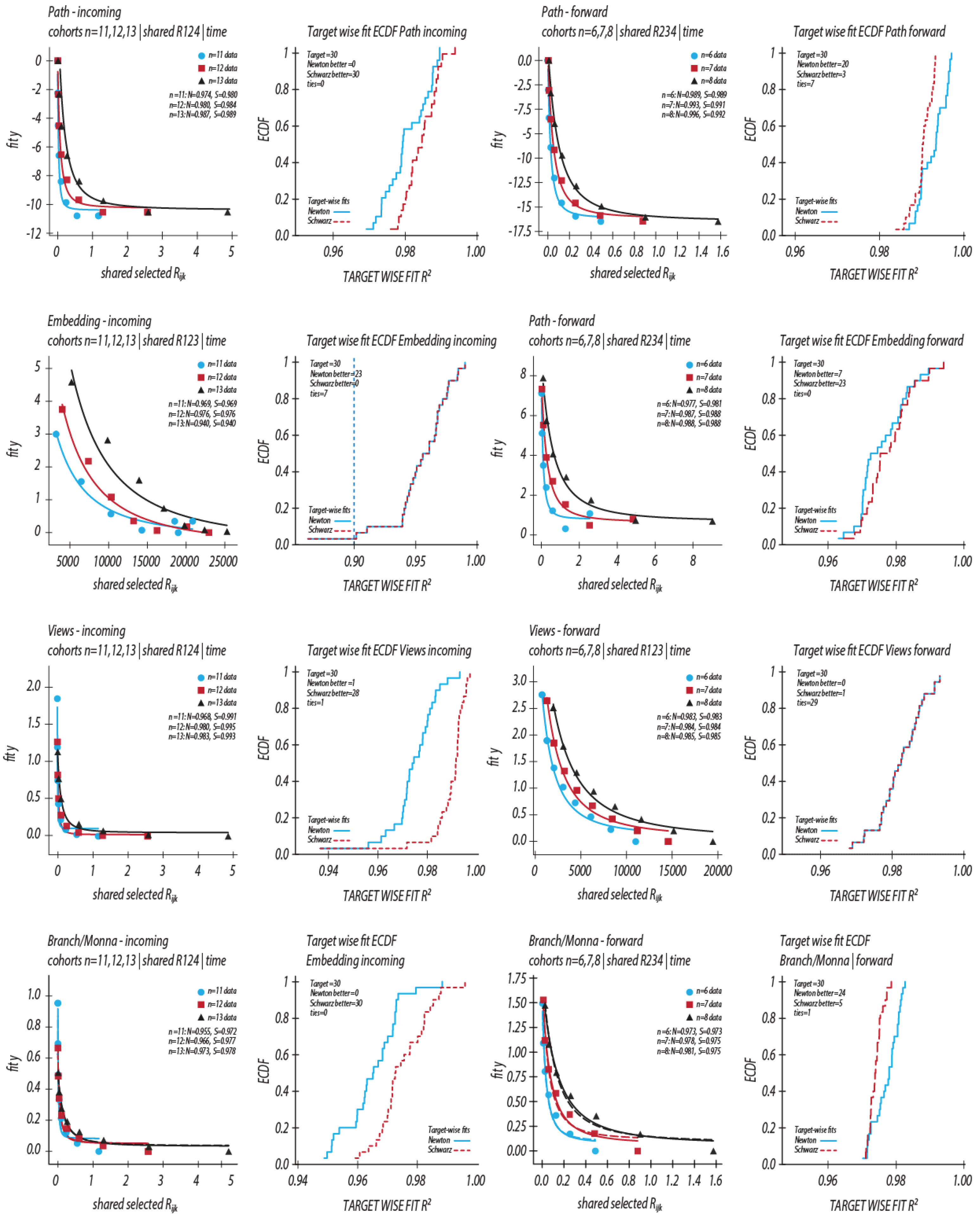
Figure 2.
Post-selection leave-one-level-out predictive comparison of the Newtonian and Schwarzschild-like informational force laws. A, overall predictive winners for the 240 individual-target trajectories and 24 cohort trajectories, classified according to the model with the lower cumulative held-out squared error. B, individual-target predictive winners for each informational representation and transformation direction. C, corresponding cohort-trajectory predictive winners. D, predictive-error difference by representation and direction; positive values favour the Schwarzschild-like model. Individual-target summaries show the median and interquartile range, while cohort summaries show the corresponding cohort-level values. In every leave-one-level-out fold, the panel-wise radial coordinate remained fixed and both force-law models were refitted to the remaining relational levels before predicting the omitted level.
Figure 2.
Post-selection leave-one-level-out predictive comparison of the Newtonian and Schwarzschild-like informational force laws. A, overall predictive winners for the 240 individual-target trajectories and 24 cohort trajectories, classified according to the model with the lower cumulative held-out squared error. B, individual-target predictive winners for each informational representation and transformation direction. C, corresponding cohort-trajectory predictive winners. D, predictive-error difference by representation and direction; positive values favour the Schwarzschild-like model. Individual-target summaries show the median and interquartile range, while cohort summaries show the corresponding cohort-level values. In every leave-one-level-out fold, the panel-wise radial coordinate remained fixed and both force-law models were refitted to the remaining relational levels before predicting the omitted level.
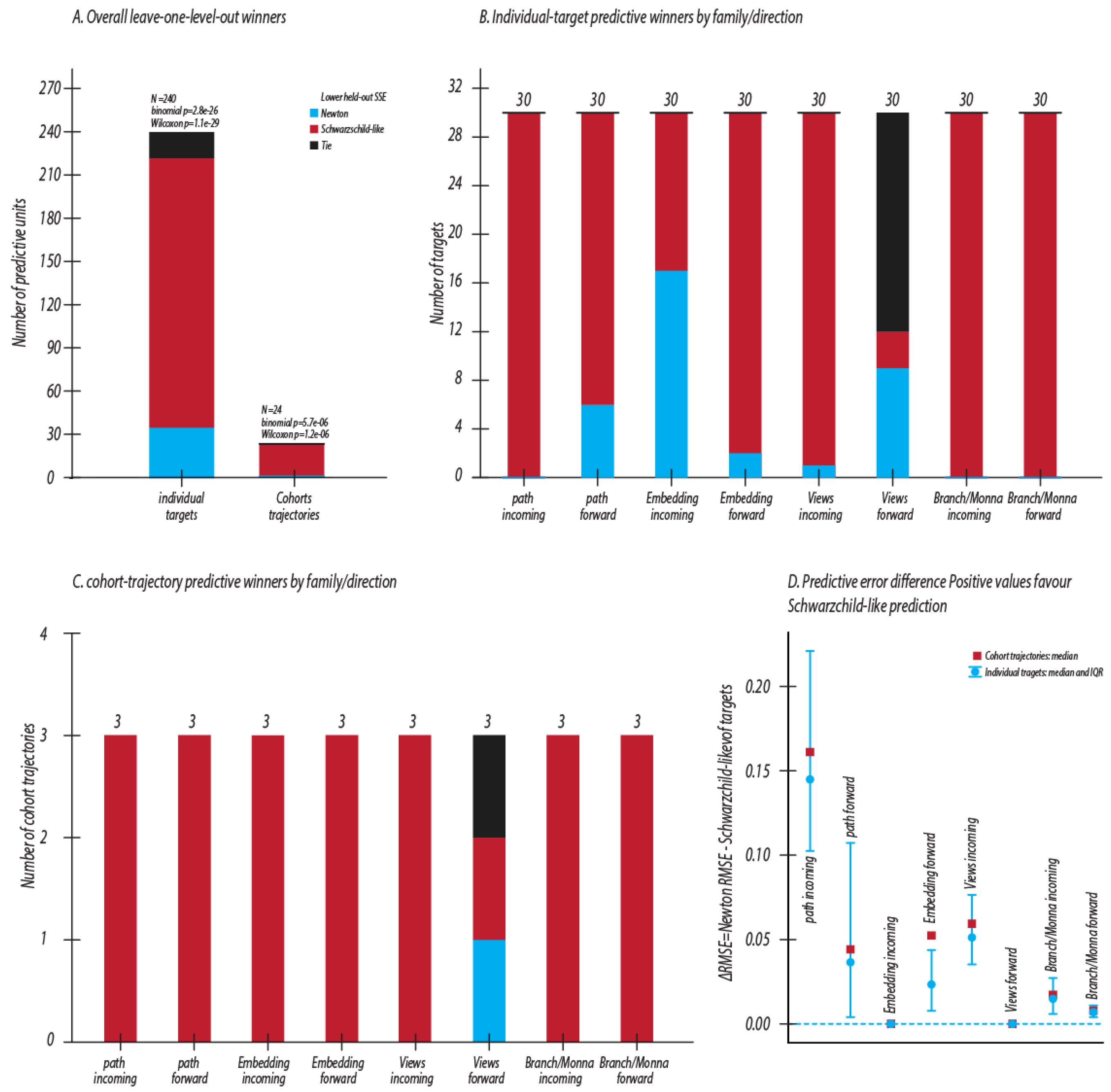
Figure 3.
Target-held-out GR-like tensor closure across the eight combinations of informational representation and transformation direction. A, Target-LOTO empirical cumulative distributions of held-out for the complete ten-component tensor (), the four diagonal components (), the six spatial components (), and the seven-component sector excluding mixed time–space terms (); negative held-out values were retained. B, median Target-LOTO across tensor sectors for each selected representation-direction model. C, median held-out versus the fraction of Target-LOTO folds with positive , jointly showing closure magnitude and target-wise coverage. The same selected model architecture was held fixed across the 30 target folds within each representation-direction analysis. Because the held-out statistics also contributed to candidate ranking, these results quantify internal held-out stability within the simulated relational ensembles rather than performance on a fully untouched external dataset.
Figure 3.
Target-held-out GR-like tensor closure across the eight combinations of informational representation and transformation direction. A, Target-LOTO empirical cumulative distributions of held-out for the complete ten-component tensor (), the four diagonal components (), the six spatial components (), and the seven-component sector excluding mixed time–space terms (); negative held-out values were retained. B, median Target-LOTO across tensor sectors for each selected representation-direction model. C, median held-out versus the fraction of Target-LOTO folds with positive , jointly showing closure magnitude and target-wise coverage. The same selected model architecture was held fixed across the 30 target folds within each representation-direction analysis. Because the held-out statistics also contributed to candidate ranking, these results quantify internal held-out stability within the simulated relational ensembles rather than performance on a fully untouched external dataset.
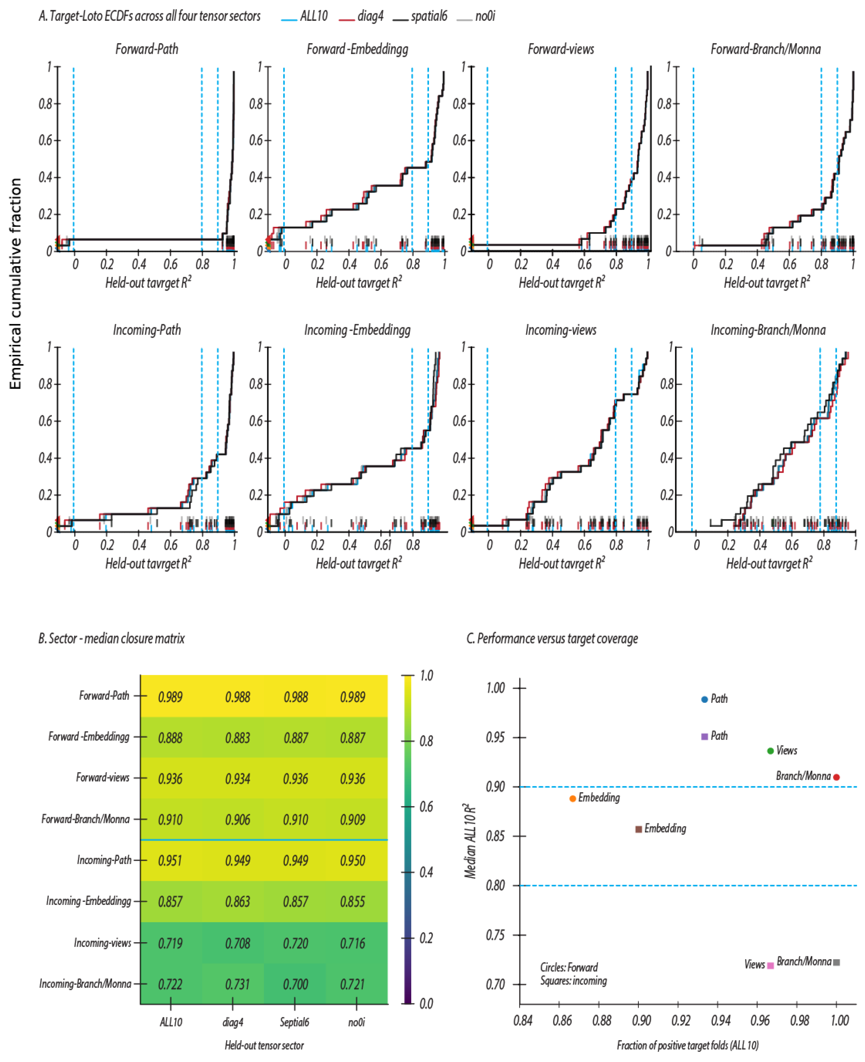
Figure 4.
Level-held-out GR-like tensor closure and selected-model architecture across the eight combinations of informational representation and transformation direction. A, Level-LOTO held-out for the complete ten-component tensor (), the four diagonal components (), the six spatial components (), and the seven-component sector excluding mixed time–space terms (). Each group corresponds to omission of one complete relational cohort. Forward analyses omit the , , or cohort, whereas incoming analyses omit the corresponding retained cohorts beginning at , , or . All reported Level-LOTO values are genuinely held out with respect to the omitted cohort. B, compact summary of the eight independently selected tensor models, showing the selected timelike coordinate, treatment of , number of targets with positive held-out , median Target-LOTO , and the spread of the median held-out across tensor sectors. All eight selected models used block-static geometry, target-median radial normalization, and the eigen radial–tangential source construction.
Figure 4.
Level-held-out GR-like tensor closure and selected-model architecture across the eight combinations of informational representation and transformation direction. A, Level-LOTO held-out for the complete ten-component tensor (), the four diagonal components (), the six spatial components (), and the seven-component sector excluding mixed time–space terms (). Each group corresponds to omission of one complete relational cohort. Forward analyses omit the , , or cohort, whereas incoming analyses omit the corresponding retained cohorts beginning at , , or . All reported Level-LOTO values are genuinely held out with respect to the omitted cohort. B, compact summary of the eight independently selected tensor models, showing the selected timelike coordinate, treatment of , number of targets with positive held-out , median Target-LOTO , and the spread of the median held-out across tensor sectors. All eight selected models used block-static geometry, target-median radial normalization, and the eigen radial–tangential source construction.
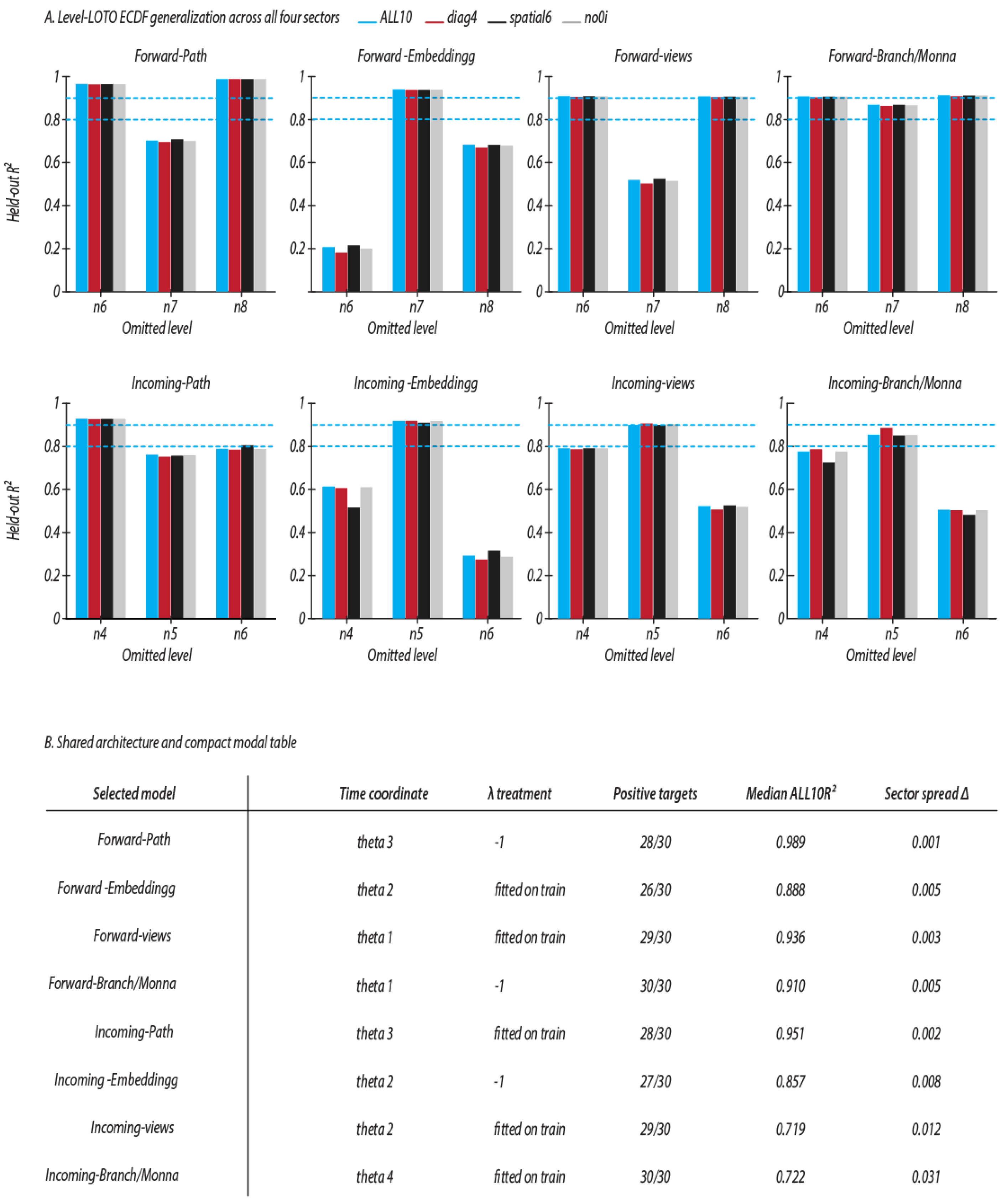
Disclaimer/Publisher’s Note: The statements, opinions and data contained in all publications are solely those of the individual author(s) and contributor(s) and not of MDPI and/or the editor(s). MDPI and/or the editor(s) disclaim responsibility for any injury to people or property resulting from any ideas, methods, instructions or products referred to in the content. |
© 2026 by the authors. Licensee MDPI, Basel, Switzerland. This article is an open access article distributed under the terms and conditions of the Creative Commons Attribution (CC BY) license (http://creativecommons.org/licenses/by/4.0/).
Copyright: This open access article is published under a Creative Commons CC BY 4.0 license, which permit the free download, distribution, and reuse, provided that the author and preprint are cited in any reuse.