

Submitted:
11 September 2026
Posted:
11 September 2026
You are already at the latest version
Abstract
We derive stellar motion, projected mass and structure formation from one objective observation field in Physical–Observation Cosmology. Its metric stress contributes real gravity and enters an inferred dark residual if omitted. The common quadratic action yields coupled collisionless and Schrödinger–Poisson evolution. Independent canonical component dilations have a positive energy Hessian, and the computed spherical responses remain bounded over the reported intervals. Across three calibrated lens cylinders, the unexplained fraction falls from 76.03% to a signed residual of \( -1.84\pm5.90 \) percentage points. For DF2, the stellar prediction is \( 7.77\pm0.64\,\mathrm{km\,s^{-1}} \); the additional-source fit is minimized at zero, although its approximate profile bound permits 57% extra mass inside the stellar half-mass radius. We prove the regional zero-residual criterion and its finite-error extension. Transferring the earlier intrinsic mode to DF4 without fitting its velocity gives \( 8.20\pm0.65\,\mathrm{km\,s^{-1}} \), consistent with \( 7.8^{+2.3}_{-2.0}\,\mathrm{km\,s^{-1}} \). The field increment is below \( 10^{-9}\,\mathrm{km\,s^{-1}} \), so this agreement tests the stellar-dominated limit. Expanding linear and nonlinear calculations then generate spatial structure from specified occupation and initial transport. A 4% periodic seed at 10 Mpc develops ordinary and field crest densities of 4.089 and 3.918 times their respective means, with new force harmonics fixed by the evolved source. Applying the environment to C0302 exposes its limits. The formal fixed-tracer monopole response is far below the required velocity change, and the unchanged infinite stellar tail develops negative remote pressure in the 10 Mpc environment. A self-consistent isolated-source refit improves the velocity residuals but requires an equivalent external column fraction of 0.433; the evolved profiles supply at most 0.00201 along a specified 10 Mpc path. The dwarf apertures require no detected independent dark component. C0302 still requires a resolved environmental and stellar-boundary solution before the same field can satisfy all of its constraints.
Keywords:
physical–observation cosmology
; dual-axis formation
; collisionless dynamics
; gravitational lensing
; coupled field evolution
; dark matter
1. Introduction
A common gravitational source is more than a mass profile at one instant. Its luminous and nonluminous components must be able to respond to one another under the equations that generated the profile. This requirement is central to Physical–Observation Cosmology: the physical state and the objective observation state enter one formation law, and their metric response must be varied and evolved together [1]. The observation axis consequently enters the source dynamics before an instrument records its effects.
The central claim is that a gravitationally inferred dark mass need not be an independent material component. An observation field contributes to the metric stress and will appear in the inferred dark residual if that contribution is omitted from the reconstruction. We derive this source attribution explicitly and test a realization in which the observation state carries the entire nonstellar source.
The preceding phase-space calculation tested the same quadratic observation mode against stellar motion and strong lensing in three galaxies [2]. Q0047–281 calibrated a common intrinsic mode coefficient. Central dispersions and lens aperture masses then calibrated H1417 and C0302. A nonnegative radial stellar population preserved the agreement in H1417 but left C0302’s predicted outer dispersion too high. That result concerns the specified stationary realization. Replacing its stellar moments by a time-dependent calculation cannot change a stationary prediction unless an actual dynamical departure from that state is demonstrated.
Here we complete the next dynamical step. The stellar distribution and the observation-field envelope evolve in their common potential. We derive the reciprocal response from the same action, establish a positive energy Hessian for independent global dilations, and construct a finite inertia response with localized radial deformations. A spherical Hamiltonian calculation then follows both components after a small, mass-preserving change in the field scale. At every time, the evolved source determines the lens aperture mass and the stellar velocity moments through the same observing geometry.
No additional gravitational coupling is fitted. The new calculation asks whether the calibrated source remains dynamically coherent and how its motion and lensing records respond to a controlled disturbance. The initial perturbation is a numerical experiment, not a measured formation history. Its consequences can therefore establish a concrete response of this realization without turning the earlier C0302 mismatch into empirical support.
DF2 extends the comparison to a diffuse galaxy whose updated stellar dispersion is already consistent with its luminous source. We use its JWST distance, HST light profile and Keck velocity summary to solve the same mode equation in a measured Sérsic potential. This tests the low-source limit and separates optical mass requirements from global field abundance. A final aperture-matched tally then records how much measured mass remains after the observation source is included.
We then extend the prediction to DF4 without using its velocity to select a field. The occupation conservation law specifies the initial data needed by this transfer. The previously calibrated intrinsic mode and a stated occupation interval determine its stellar dispersion, projected source mass and variational response together. This makes the strength of an unused-target agreement depend explicitly on how much the tested observable responds to the field.
The diffuse solution also motivates an explicit large-scale evolution. We derive the expanding common-source equations from the same action and solve their coupled linear formation stage for compensated initial perturbations. This connects a time-dependent spatial distribution to specified initial data and shows why a cosmological field cannot be identified with a superposition of isolated dwarf envelopes. A periodic plane-symmetric solution then follows the same nonlinear equations beyond the weak-contrast regime. Its density harmonics determine the force and tidal field without an additional source adjustment. We finally apply that environment to C0302 and resolve the galaxy field again to determine which environmental column its velocity data would require. This connects the formation calculation directly to the unresolved observational test.
2. Two States, One Metric Source
The monograph’s Einstein-representable branch uses, in natural units,
Here s is the objective observation state, its intrinsic quotient metric and its kinetic normalization. Metric variation and state variation belong to the same functional. In particular,
The source normalization is the same on both axes. Ordinary angular projection, seeing and spectral response act later, on records generated by this source. They do not supply an independent gravitational term.
At a stationary intrinsic state, a positive normal mode obeys with . We retain the compatible quadratic restriction , whose one-mode embedding is geodesic with tangent potential gradient. The monograph identifies these conditions as the bridge from a stationary branch to a dynamically closed reduction [1]. Its numerical mode coefficient is a property of that specified realization and is calibrated from data; it is not fixed by the dual-axis structure alone.
Carrier averaging in the weak, nonrelativistic regime gives . The stellar mass distribution and the envelope then satisfy
The potential is local, with the cosmological background subtracted; we use isolated boundary conditions and omit expansion and external tides. The retained minimally coupled source has equal weak metric potentials at leading order, so this same determines the nonrelativistic acceleration and light deflection.
For isolated boundaries, each component’s mass is conserved. The energy is
Writing and gives for either kinetic energy. Poisson symmetry gives . Thus : mutual response follows from the common source, with no separate feedback coefficient.
For a stationary real envelope , the first variations take the form
where and the carrier of the stationary envelope has been removed. Setting removes an entire response in the last two equations. It is the fixed-stellar-source approximation, rather than the full coupled perturbation problem.
3. Coupled Radial Response from the Common Energy
The stellar distribution and the formation envelope respond to the same potential. Their interaction can therefore be followed without assigning a separate force to either component. Let denote the random stellar kinetic energy, the envelope gradient energy, and the enclosed mass. In the spherical sector the conserved energy is
where . The field mass is . We first examine a family whose energy curvature can be obtained exactly, then construct localized displacements with finite inertia.
3.1. Independent Canonical Dilations
The stellar transformation is symplectic. It preserves the mass, the distribution’s positivity, every phase-volume Casimir, and each stellar angular momentum. Its density is and its kinetic energy is . The mass-preserving field dilation similarly gives . Let and denote the negative self-gravitational energies. The exact energy along these two independent dilations is
The shell expression retains the motion of the boundary separating interior from exterior shells. Define
Then at unit dilation, and differentiation gives
Stationarity supplies the separate virial identities and . Substituting them in the second derivative of Eq. (7) yields
For a nontrivial stellar population and a nontrivial envelope this matrix is positive definite, since
The overlap energy thus opposes relative dilation. This is an exact positive-curvature result for a family that preserves the stellar phase-space structure and the field occupation.
A global dilation nevertheless does not define a finite-energy breathing motion for the adopted stellar profile. Its bulk inertia is , while at large radius. The integral diverges. The static curvature in Eq. (10) remains finite, but a nonzero global expansion speed would carry infinite kinetic energy. A finite dynamical calculation must localize the displacement in both its energy and its inertia.
3.2. Localized, Dynamically Accessible Displacements
For each component choose a radial displacement and the monotone map
The stellar cotangent lift sends and . It is canonical in Cartesian phase space and preserves the same Casimirs and angular momenta as the global transformation. The perturbed population is the transported initial distribution; it is not replaced by a new equilibrium distribution after displacement. Writing , its kinetic curvature is
All velocity moments in this expression come from the same stationary and common potential used for the observational calculation.
The field shell masses are preserved by . For the real stationary envelope this gives the exact finite-deformation energy
Its second derivative is
The derivatives of account for the changing radial Jacobian; they cannot be omitted when a global dilation is localized.
Shell ordering is preserved by the deformation. The self energy becomes
Applying the displaced-shell calculation to the cross term yields
The full diagonal entries are and . Equivalently, the gravitational quadratic form contains the overlap contribution , which vanishes for a common displacement. Equations (13)–(16) recover Eq. (10) when both displacements equal r.
We use the smooth trial shapes
They approach a dilation near the centre and decay as at large radius. Their derivatives are and , with . The declared localization scale selects a response shape; it changes neither the formation law nor its calibration parameters.
3.3. The two-component radial response
A radial bulk velocity is generated by a canonical momentum translation. For the envelope the corresponding phase is , where . At quadratic order the symplectic term is and the bulk kinetic energy is , with finite inertias
Thus the coupled response follows from
Holding the stars fixed gives for the same field displacement. Allowing them to respond instead gives
The stellar contribution is frequency dependent. In the static positive-stiffness limit it reduces the field stiffness to the Schur complement ; dynamically it splits the two coupled response frequencies.
This construction is a Hamiltonian variational restriction of the coupled stellar–field dynamics. Positive eigenvalues establish oscillatory motion within this two-displacement restriction. The full kinetic system also contains phase mixing, orbital resonances, and perturbation shapes beyond this finite basis. The direct evolution calculation examines the stellar and field distributions themselves. Both calculations retain the same instantaneous mass perturbation,
which governs acceleration and lensing together. No independent lensing response is introduced.
4. A Spherical Evolution of Both Components
4.1. Initial States and a Controlled Displacement
We retain the stellar density
and use the positive phase-space distribution
The angular momentum is per unit stellar mass. The distribution vanishes for . For this density, the augmented-density Abel inversion is nonnegative throughout the stated interval for every positive, nondecreasing finite enclosed mass [2]. The actual includes the stationary formation field. Velocities are sampled from this distribution, including its non-Gaussian tails, rather than from a Gaussian with the same second moment.
Let , and . With and radial envelope u normalized by , the field equation is
The initial nodeless solution has , where
Once the evolution starts, the stellar contribution is recomputed from the evolved distribution at every step.
The common mass is fixed at the median CDF node of the previous calibration, . For each galaxy we select a stored conditional state near the posterior medians of , and , within the region whose calibration is no larger than the number of calibration measurements. The target outer velocities do not enter this selection. These three states are representative calculations, not a new posterior integration or a refit of the discrepant outer measurements.
Each initial state is evolved twice. The control starts at the stationary field and stellar distribution. The disturbed run changes only the field scale,
while using the identical stellar realization. This deformation preserves field mass and introduces no new source law. The subsequent stellar response is generated by Eq. (3). Taking the difference from the paired control isolates the response from finite sampling and initialization effects. The perturbation amplitude is specified before the evolution and is not optimized against C0302.
4.2. A Reciprocal Discrete Hamiltonian
Equal-mass spherical phase-space shells represent the stellar population. Each shell carries a radius, radial velocity and angular momentum; a Cartesian representation integrates its central-force orbit through pericenter. Its angular orientation is averaged when constructing the spherical force and observables. This calculation retains radial collective response and does not evolve nonspherical multipoles.
For N stellar shells, , and wave masses at radii , the dimensionless gravitational energy is given below. In these discrete expressions, all radii are in units of b and velocities in units of :
The sorted stellar radius is . The empirical stellar pair sum omits its diagonal self-interaction; this is a convergent quadrature of the continuous collisionless energy, with no artificial central self-force on an individual sample. Differentiating the energy with respect to stellar position gives the interior stellar mass and the interior wave mass as the central acceleration. Differentiating with respect to the wave amplitude gives the stellar and wave potentials on its grid. This common derivative fixes the reciprocity of the two components at the discrete level.
The stellar kinetic energy is and the wave kinetic energy is , with zero boundary values. A symmetric potential–kinetic–potential splitting applies a half stellar velocity kick and wave phase rotation, followed by a full stellar drift and sine-transform wave step, and then the second half potential step. Density and positions are constant during each potential flow. The wave kinetic phase uses the eigenvalues of the same discrete Laplacian that selected the initial field. Consequently the scheme preserves wave norm and the spherical specific angular momenta, with a symmetric Strang splitting of the common Hamiltonian. Shell crossings make its force piecewise smooth; the accuracy of the complete trajectory is therefore assessed by direct resolution comparisons.
The stellar radii follow the exact inverse cumulative law , with z drawn from a scrambled Sobol sequence. There is no outer stellar cutoff. The conditional speed distribution is obtained from the positive Abel inversion after rescaling tangential velocity by . The numerical stellar potential includes shells beyond the wave grid, while the exterior wave force uses its full enclosed mass. This treatment preserves the finite-mass tails without confusing the wave box with the extent of the stellar system.
5. Motion and Lensing Along the Same Trajectory
The source used for the records is the evolved source itself. Holding the old luminosity weights fixed while moving stellar mass would discard part of the physical response. We instead retain a constant stellar mass-to-light ratio and use the instantaneous stellar distribution for both the luminosity and velocity-moment fluxes. Radii and velocities in this section have their physical units restored before projection.
Let be the azimuthally averaged acceptance of a slit extraction, including its point-spread function and offset. With angular scale ℓ in physical length per arcsec, define
For a stellar shell with radial velocity and total tangential speed , averaging over its orbital orientation gives
The coefficients follow from and for the tangential velocity direction. Front–back symmetry cancels the projected mean even during a spherical radial flow. Thus and use central as well as raw even moments. The spectra’s instrumental line-spread function would be applied after this intrinsic velocity projection.
For a shell of radius r, its fraction inside a cylinder of radius R is
The same evolving wave and stellar masses therefore give the instantaneous deflection . The half-mass radii of both components provide a complementary measure of the source motion. No equilibrium Jeans equation is imposed after the disturbance; the stellar velocities in Eq. (29) have been evolved explicitly.
We preserve the slit widths, signed or folded extraction bins, lens radii and selected nuisance geometry of the previous calibration. The underlying Hubble imaging and Keck stellar measurements are those of Refs. [3,4]. The lens constraints remain compressed image reconstructions, rather than a new pixel-level lens fit. In particular, time dependence is a computed response and is not an observed time series for these galaxies.
6. Coupled Modes and the Direct Evolution
The selected states in Table 1 have the same intrinsic mode and different occupations and stellar confinement. Their global dilation Hessians are positive, as required by Eq. (11). More strongly than a numerical sign check, that identity shows why the overlap cannot be represented as an arbitrary attractive or repulsive correction: its coefficient is fixed by the two radial mass gradients, and it penalizes relative dilation.
The finite-inertia calculations also give positive eigenvalues for all three objects and all three declared localization scales. The resulting 18 squared frequencies are positive. Table 2 lists the two periods at each scale. For C0302 at , holding the stellar displacement fixed would give a field period of Myr. Allowing the stars to respond gives periods of and Myr. The associated stellar-to-field displacement ratios are and : the slower response moves the components together, while the faster response moves them in opposite directions. These are the two responses of the declared variational restriction, with no new force coefficient.
The direct evolution releases the two-displacement restriction and advances the sampled stellar distribution and the radial field. A 5% initial field expansion produces an oscillatory response in both components, as shown in Figure 1. The stellar half-mass radius remains unchanged at the instant of the field displacement and then begins to respond. This behavior follows directly from the initial conditions. If and the field alone produces , velocity integration of Eq. (5) gives
The field first changes the force; stellar redistribution follows through its acceleration and continuity equations. Its initial density response is quadratic in time. This delayed physical redistribution is distinct from spatial smoothing in an instrument.
The simulations cover : approximately 235 Myr for Q0047, 538 Myr for H1417 and 543 Myr for C0302. Over these intervals, the disturbed half-mass radii remain bounded, and the unperturbed controls remain close to their initial configurations. The largest changes relative to the controls are given in Table 3. This is a finite-duration result for the specified radial perturbation. It establishes that a live stellar response can be followed consistently in these selected realizations; it does not establish stability against every distribution-function perturbation or nonspherical disturbance.
Figure 2 shows why dynamical consistency and observational agreement are separate questions. C0302’s lens aperture mass and stellar moments change together along the same trajectory, but the outer dispersion remains approximately 258.1–267.1 . Its largest paired change is 5.2 , whereas the observed outer mean is . The initial discrepancy is much larger than the response to this perturbation. The experiment therefore does not turn the stationary C0302 realization into an explanation of its measured profile.
The characteristic times are millions of years, so these curves are not proposed as telescope monitoring targets over a human observing baseline. Their role is to test the dynamical admissibility and correlated response of candidate source states. The corresponding observational tests remain simultaneous spatially resolved motion, fourth velocity moments and lensing, evaluated with the response and uncertainties of those observations.
7. Mass Fractions and Independent Dark Matter
7.1. Gravitational Source Attribution
An additional gravitational source does not uniquely imply an additional material species. This statement follows from the common metric equation. To make the attribution explicit, suppose an independent dark component were present and define the stress inferred after subtraction of the stellar source:
This identity holds when all tensors refer to the same metric and source convention. A reconstruction that omits the observation stress assigns that stress to its inferred dark component. In the nonrelativistic branch of this paper it reads
Consequently is entirely compatible with a positive inferred dark mass. The chosen realization gives that mass a definite origin: the gravitating energy of the objective observation state. The origin is carried by an evolving source, rather than supplied by the name assigned to a residual.
The theoretical conclusion is direct. Assigning a unique material identity to the additional source on the strength of its gravitational residual alone is an underdetermined inference. Equation (32) exhibits the missing source term explicitly. Which allowed source actually accounts for a galaxy is then decided by its common solution for motion, lensing and evolution. The preceding C0302 comparison applies that requirement to the present realization.
7.2. Before and After Including the Observation Source
The source attribution can be quantified with the same galaxy, aperture and stellar parameters. At fixed tracer density and orbital anisotropy , let . The stationary radial pressure obeys
Projection through a fixed aperture is linear in this pressure, and its luminosity normalization is fixed by . Thus
Here is the contribution of the observation source to the stellar velocity variance. It is not a separately measured velocity distribution of the field. Equation (34) is used only for this comparison of stationary sources, before the live evolution begins.
Table 4 and Table 5 implement the comparison at the selected parameters. The stellar density, mass, orbit family, slit geometry and lens radius are held fixed. The stellar column omits the observation contribution; the common-source column includes the previously calibrated field. This operation isolates the size and direction of its gravitational effect. It is not a refit of a historical dark-halo model with different stellar parameters.
If only the stellar term were included in reconstructing the common model’s source, the inferred missing cylinder mass would be exactly . Accounting for the observation state transfers that entire quantity from the unexplained residual into an explicit field source. This before-and-after comparison establishes the observation contribution within the constructed realization. The measured columns supply the separate empirical comparison: C0302’s common-source dispersion is still excessive, even though the field supplies much of its lens cylinder mass. The change in source attribution and the accuracy of a galaxy fit are therefore both visible in the same tables.
7.3. The Residual Fraction
The mass budget separates two meanings of an observation contribution. Seeing, aperture weighting and spectral response change the recorded signal. The observation state in Eq. (2), however, carries energy and sources the metric. Correcting an instrumental record does not remove that source. To ask how much independent dark matter remains after accounting for the observation state is therefore to ask for a decomposition of the gravitating mass.
If an independent component were admitted, its bookkeeping would read
For a common enclosing radius, the corresponding residual fraction is
Every term must refer to the same three-dimensional sphere. A lensing version instead uses cylinder masses throughout; mixing a cylinder mass with a spherical mass does not define a physical residual. Moreover, is itself inferred through a source and orbital model. Equation (37) specifies what must be determined, without supplying an extra independent measurement.
At a fixed stellar distribution, the instantaneous motion and lensing records depend on the common potential. A redistribution , leaves that potential unchanged whenever the redistributed sources are admissible. Gravity alone then measures their sum. The specified field equation restricts which observation profiles and histories are allowed, so a joint dynamical calculation can help distinguish components only after their independent profiles, evolution and admissible parameter ranges have also been specified. The present calculation introduces no such independent component and fits no such enlarged decomposition.
Its precise hypothesis is
Thus the independent-dark-matter fraction is zero by the tested hypothesis, not a percentage measured to be zero by these data. No numerical residual fraction beyond the observation source has yet been identified by this fit. A negative residual would indicate an incompatible decomposition or its uncertainty; clipping it to zero would not establish the absence of an independent component.
The selected realizations do give definite fractions for their own source budget. Since , their globally integrated observation-source fraction is :
| Galaxy | Observation source | Stellar source |
| Q0047–281 | ||
| H1417 | ||
| C0302 |
These are fractions of the finite total masses of three selected galaxy solutions, including their extended tails. They are neither cosmic abundances nor aperture fractions, and they are not posterior bounds on a residual dark component. In particular, C0302 already has an outer dispersion above its measured value. Within its fixed source and orbital closure, this discrepancy is not evidence for additional positive missing mass. The common-source hypothesis must explain the observed records before its mass decomposition can acquire that empirical interpretation.
8. DF2 at the JWST Distance
DF2 tests a different limit of the same equations. Its low stellar velocity dispersion leaves little room at the central measured value for a positive additional force. We retain the intrinsic mode selected in the lens calculation, replace the stellar source by DF2’s measured light profile, and solve the field equation again. The conserved amplitude remains specific to the galaxy. This transfers a physical coefficient between systems without prescribing equal field abundances.
8.1. Distance, Light and Stellar Motion
The JWST/NIRCam red-giant-branch-tip measurement gives Mpc, or distance modulus mag [8]. Program 3990 supplied F090W and F444W exposures of 12 626 s each, and F150W and F356W exposures of 1031 s each. This is a distance measurement from imaging. The velocity information comes from Keck/KCWI.
The HST light profile has Sérsic index , major-axis effective radius , and projected axis ratio [9]. Its circularized radius is . We adopt the spherical deprojection of this circularized profile and constant stellar mass-to-light ratio. The published total stellar normalization is at Mpc. Therefore
where is in radians in the second expression. The JWST central distance gives and kpc. The same distance enters both quantities. The population-model uncertainty of 0.07 dex is retained once; the correlated published mass-to-light estimate is not a second constraint.
The latest broadening-corrected KCWI estimate gives the gravitational dispersion [11]. It accounts for stellar line broadening of and binary broadening of through subtraction of their variances. These corrections are already included in the adopted dispersion. Danieli et al.’s original article gives [10].1 This is the earlier analysis of the same spectra. The historical mass comparison, at Mpc and kpc, was against . Those derived masses supply context; the new calculation uses the single updated velocity summary.
The integrated KCWI measurement covers a rectangle just southwest of the centre [10]. We approximate its placement using the published velocity-map geometry: the centre is west and south of the galaxy centre. A Gaussian seeing FWHM of is adopted for projection and varied from to . Exact extraction masks and weights are unavailable in the published summaries, so this is a figure-derived aperture approximation. It is not a circular half-light-radius measurement.
8.2. A Finite-Mass Source Derived from the Light Profile
Set and normalize the projected stellar profile to unity:
Its exact spherical density, cumulative mass and potential are
The physical stellar density is . For its centre is finite: . The numerical deprojection gives and at . Thus kpc and .
The same stationary observation equation becomes
The subscript on distinguishes the effective-radius unit from the Hernquist scale used for the lenses. At the physical observation envelope vanishes; its normalized linear eigenfunction defines the limiting response. No nonzero abundance is imposed at this boundary.
For an isotropic stellar population and a nonnegative aperture response W, define
Here W is the azimuthally averaged, PSF-convolved rectangle, in effective-radius units. Integrating the isotropic Jeans equation and interchanging its two positive radial integrals gives
The normalization and numerator use the same response. The inequality is exact at fixed stellar and orbital parameters: this branch’s observation source can only increase the stellar second moment.
The isotropic phase-space realization can also be checked directly. With and , Abel inversion is nonnegative if
Its boundary term vanishes for the exponentially declining stellar tail. Differentiating the integrand of Eq. (41) verifies this sufficient condition across the stellar body and tail for , together with positive central and asymptotic limits. This establishes more than positivity of a Jeans variance at the sampled source states.
8.3. The Measured Low-Dispersion Limit
The aperture integrals give
The stated uncertainty propagates the stellar-normalization and JWST-distance summaries, with . It does not include departures from spherical isotropy or population-model systematics. The central prediction is only of the quoted upper velocity error above the updated measurement. Centering the rectangle changes it to ; the tested seeing and one-arcsecond placement variations give –. Using the alternate HST TRGB distance Mpc [8] gives a central prediction of , still consistent with the velocity summary. We retain the JWST distance as the primary case and do not average the discrepant distance determinations.
Equation (42) explains why a large global field fraction need not appear as a large optical force. In the weak-amplitude, limit, the mode mostly samples the stellar Kepler tail:
For while the field remains diffuse, the rescaling instead gives . Self-gravity therefore eventually makes the optical contribution large, as Table 6 demonstrates. The likelihood is almost flat over modest global amplitudes and excludes sufficiently large ones within this isolated ground-state family.
The very diffuse solutions also extend beyond a galaxy’s dynamical domain. At the field half-mass radius is 11.35 Mpc. Such a formal isolated equilibrium does not supply a formation history or an environmental boundary condition for DF2. The zero-envelope solution has neither requirement and already explains the measured stellar dispersion. We therefore infer a low optical source requirement, without assigning a measured galaxy-wide field abundance.
The same computed source fixes a lensing prediction through the cylinder projection of . At , for example, , while the field mass projected inside is . The stellar cylinder contains . Their difference from the spherical budget arises from the extended line-of-sight source. These are common-field lensing predictions; DF2 has no lensing likelihood in this calculation.
Sérsic stars have finite global dilation inertia, so the positive two-component Hessian derived earlier now directly admits finite global variational periods. The same state gives and Gyr. These characterize the stated canonical displacements of its equilibrium. The DF2 comparison contains no observed time series and no new live-evolution trajectory.
8.4. How Much Additional Source Remains Allowed?
Define the optical fraction in the spherical stellar half-mass radius by
We use the published asymmetric velocity errors to construct the explicit approximate discrepancy function
Distances and velocities in this expression use Mpc and . This is a summary-based Gaussian approximation, rather than a reconstruction of the spectral posterior. The profile minimum over occurs at .
For the upper contour, the diffuse core permits , with and . Profiling and D gives
The contour uses the usual one-sided Gaussian 95% convention; its coverage has not been calibrated against the unavailable spectral likelihood or structural systematics. At its profiled nuisance values, the full field solution reproduces the core velocity prediction to 0.032%. Holding the stellar mass and distance fixed instead gives at the same contour, with . The allowance is broad despite the zero-source minimum.
Figure 3.
Left: the field solution increases the dispersion only when its global amplitude is large enough to concentrate appreciable mass within the stellar body. The shading shows the published asymmetric Keck error interval, the dashed line its centre, and the dotted line the stellar-only prediction. Right: profiling distance and stellar normalization gives a zero-extra-source minimum and a broad upper allowance. The crossing is an approximate Gaussian summary convention, conditional on the stated spherical core model.
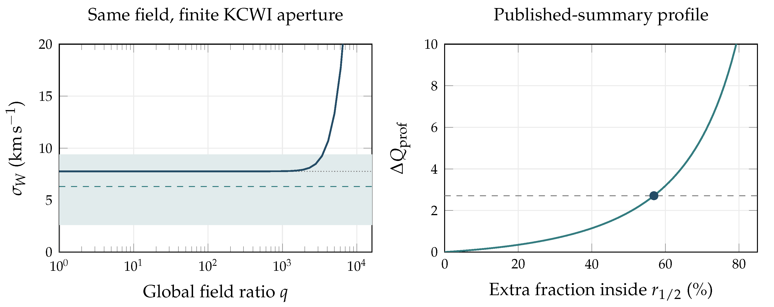
An independent additional component would enter the same positive kernel. If its optical density shares the fitted core shape, the velocity summary constrains the sum of its amplitude and the observation-field amplitude. After a specified observation contribution is subtracted, the remaining independent fraction lies between zero and the allowed total extra fraction; it is not separately identified along that amplitude degeneracy. Equation (50) is therefore a useful approximately 57% optical allowance for an extra source of this shape, alongside a best fit at zero. It is neither a positive detection nor a model-independent bound on all possible mass profiles. The amplitude degeneracy concerns the optical response. A global equilibrium containing an independent third component would also require solving Eq. (42) in its additional potential.
9. The Remaining Source in the Measured Apertures
9.1. A Zero-Residual Criterion for an Independent Dark Source
The source-attribution identity acquires an exclusion meaning when the residual is combined with positivity. We work in the additive, nonrelativistic mass-source regime of Eq. (3) and write a possible complete source as
Here includes all ordinary matter admitted in the target, and denotes an independent component beyond the observation field. The preceding stellar models approximate by . A physical exclusion also requires any relevant gas, remnants and other ordinary sources to be included in that budget. All terms use the same volume, gravitational normalization and boundary conditions.
Proposition (zero residual).
Let be a nonnegative integrable density on a measurable region V, and suppose Eq. (51) exhausts the mass source there. Define the exact residual
Then
If the density is continuous, it vanishes at every interior point of V.
Proof. Choose an arbitrary positive density scale and put . Nonnegativity gives
Every has zero volume. Their countable union is the set where the density is positive, proving the forward implication. The reverse follows by integration. A positive value at a continuous interior point would remain positive on a small ball, contradicting the zero integral.□
Thus an exact zero residual can exclude an independent positive mass source in a specified region. The conclusion requires a complete and correct source subtraction; it cannot establish that subtraction from the residual alone. An exact negative residual would instead contradict Eq. (51) for the specified sources. It could not be repaired by adding a nonnegative dark density.
9.2. Finite Precision and the Observing Kernel
Let be the measured residual. Suppose a joint uncertainty construction gives on a stated coverage event, including errors in the ordinary source, observation source and gravitational reconstruction. On that event,
provided the upper endpoint is nonnegative. A negative upper endpoint leaves no compatible nonnegative mass under the stated model and uncertainty event; setting it to zero would conceal that incompatibility. A Gaussian standard error supplies a probabilistic interval at a chosen level, rather than a deterministic error bound. Correlations created by source calibration enter the same uncertainty construction.
For measurements that weight the source rather than integrate it over a sharp region, the corresponding statement is
Assume these products are integrable and the set of measurements is finite or countable. If every vanishes exactly, the same positivity argument excludes dark density almost everywhere on the union of the regions where at least one is positive. A lens-cylinder mass uses the indicator of that cylinder. The fixed-tracer Jeans response in Eq. (44) gives a nonnegative kernel on density after the radial integration order is exchanged. A finite-error bound on a total regional mass also requires quantitative coverage. For example, if on V, with , and the residual upper bounds hold jointly, then
This relation makes the spatial support and sensitivity of an exclusion explicit.
The theorem supplies the mathematical interpretation of the observations below. The lens residuals in Table 7 overlap zero, and the pooled percentage-point result is a finite-precision, fixed-source comparison. Its negative centre is compatible with measurement scatter and does not invoke the exact-negative contradiction. DF2 reaches the zero-extra-source boundary, while Eq. (50) retains an approximately 57% allowance for the stated optical core model. It can therefore be described as a candidate for a galaxy without an independent dark component in the region probed by its stellar kinematics. Neither comparison has established the exact premise of Eq. (53).
The decisive physical step is to determine the observation stress from the common action and test its source prediction with independent records. Merely omitting an independent component from an assumed action selects the zero-dark-matter hypothesis. The dual-axis structure itself permits different constituents within the physical state and does not prohibit a nonluminous constituent. For a global additional component, the observation field must also be solved in its gravitational potential. The criterion applies to each complete, self-consistent source decomposition, with its actual observing kernels and uncertainties.
9.3. The Measured Remainders
The final comparison subtracts both specified sources from the measurement, within the same aperture. For a strong lens, define
A positive value denotes unaccounted cylinder mass at the selected parameters. A negative value denotes an overprediction, and is retained with its sign. It cannot be interpreted as a negative matter abundance. At fixed source prediction , the measurement-only linear uncertainty is . The residual significance is evaluated in the original measured mass, .
For Q0047, the outer velocity prediction is , against , and the lens cylinder prediction is , against . Their residual magnitudes are and standard errors. The two other velocity apertures give and , against and . All three apertures are within one quoted error. These measurements participated in calibration, so their close agreement describes the fitted solution.
The outer-velocity analogue of Eq. (58) is . For Q0047, H1417 and C0302 its central values are , and . This is a second-moment residual; its radial kernel prevents its identification with a generic enclosed mass fraction. In the original velocity variable the signed discrepancies are , and quoted errors. C0302’s small positive lens-mass residual therefore coexists with substantially excessive predicted outer motion. Adding a positive source at fixed stellar and orbital parameters cannot cure that discrepancy.
None of the three lenses has a positive mass residual above two quoted measurement errors. DF2 also has no significant positive velocity residual: its additional-source optimum is at zero, with the allowance in Eq. (50). Thus the four objects yield zero significant positive excesses in the reported comparisons. This is a count within a selected sample. The aperture masses, their calibration dependence and the DF2 summary approximation do not define a universal dark-matter mass fraction or a population detection rate.
The mass-only tally is given by the sum of the three actual lens cylinders in Table 7; DF2 is excluded from that sum because it has no measured cylinder mass. The quoted errors hold the selected fields fixed and omit their stellar, orbital and calibration covariance. The tally makes the remaining source discrepancy explicit, while C0302’s outer motion tests the validity of the source that was subtracted.
10. A Fixed-Parameter Prediction for DF4
A predictive observation field must carry its gravitational source from one calculation into the next. Reconstructing a residual after measuring the motion is insufficient: the field equation must first determine a source, and that source must then produce the measured record. DF4 provides a target unused in the preceding calibration. We retain the intrinsic mode and propagate a specified range of previously calibrated occupations, without adjusting either to DF4’s velocity dispersion. The resulting comparison also makes a useful distinction between predicting a stellar-dominated limit and detecting the field itself.
10.1. Conserved Occupation and Predictive Initial Data
The observation field is an objective structure with metric stress (2). Its quadratic, nonrelativistic reduction permits a direct statement about how much of that structure the dynamics fixes. Multiply the wave equation in (3) by , subtract the conjugate equation, and use the reality of . The potential terms cancel, giving
Consequently, for a fixed spatial volume V,
An isolated solution with no flux at infinity conserves and . The field equation determines the spatial distribution and its subsequent response at a specified occupation; it does not replace that conserved initial datum by an algebraic function of the stellar mass.
This result can also be seen in the stationary normalization. With , write
Unit normalization of u fixes a shape convention; it neither sets nor selects q. Minimizing the energy at fixed N determines a stationary shape within that mass sector. Moreover, if , positivity and conservation imply almost everywhere for every time on which the isolated reduced solution exists. Thus this branch does not generate a nonzero field from zero occupation merely because a stellar potential is present. A source flux, a populated initial state, or dynamics beyond this closed reduction is required.
The monograph’s Internal Source Determination Edition places this initial-value statement within the full two-axis formation law [12]. Reconstruction of an action along a specified connected history and evolution of specified initial data are distinct operations. In the one-dimensional reconstruction, the known history fixes and on its monotone traversed interval. Here and are the source and kinetic reconstruction functions defined in that construction. These relations determine the action on that history; they do not identify every galaxy’s occupation with the action’s kinetic normalization. Equations (59)–(61) give the corresponding result inside the retained quadratic branch.
For the present transfer we therefore specify the prediction rule explicitly. The intrinsic coefficient remains . The three earlier selected occupations are , , and , from C0302, Q0047, and H1417, respectively. All three values and an intervening logarithmic grid are propagated to DF4. This interval is a transfer assumption, not a probability interval or a theoretical upper bound. No DF4 velocity parameter is fitted. Because DF4’s low dispersion was already publicly known when the target was chosen, the exercise is a retrospective prediction for an unused target, rather than a blinded observation.
10.2. The Stellar-Window Prediction
The HST light profile gives , , and projected axis ratio [9]. We use its circularized spherical deprojection, constant stellar mass-to-light ratio and isotropic equilibrium. The HST tip-of-the-red-giant-branch distance is Mpc [13]. Rescaling the photometric stellar normalization, at Mpc, gives
The alternative HST surface-brightness-fluctuation distance of Mpc is used only for sensitivity [8]. The cited distance table contains no JWST distance for DF4; DF2’s JWST result is not transferred between the two galaxies.
The KCWI observations cover a dithered region centred on DF4 [14]. We approximate that footprint by a uniformly weighted rectangle convolved with a Gaussian of FWHM. The seeing is an assumed projection parameter. The published data involve masked clusters and weighted exposures, so the rectangle represents the coverage rather than an exact reconstruction of the extraction mask. The positive kernel in Eq. (43) then gives, for the newly solved field,
The stellar coefficient is . Across the specified occupation interval the resulting dispersion is
The quoted prediction error propagates the 0.06-dex stellar normalization and the distance error once, using at fixed angular profile. It does not include the full uncertainty in orbital structure, stellar populations or the environment. Varying the adopted seeing, rectangle and centre in the specified sensitivity cases changes the stellar prediction from to ; adopting the alternative central distance gives .
Only after this forward calculation do we compare the updated stellar measurement,
This estimate accounts for binary broadening. It updates the earlier result from the same spectra [14]; the two values are not independent measurements. The prediction exceeds the updated central value by only . Dividing by the quadrature sum of the upper observational error and the quoted photometric prediction error gives , a summary measure of compatibility rather than a probability calculated from the full likelihood.
Figure 4.
The unused DF4 velocity summary and the fixed-rule prediction (left), followed by the contribution of the solved field (right). The prediction error includes only stellar normalization and distance; the measured errors are the published asymmetric summary. The entire transferred field interval is indistinguishable from the stellar-only prediction on the left. Points on the right mark the three historical occupations; the curve is a sensitivity sequence, not a fitted posterior.
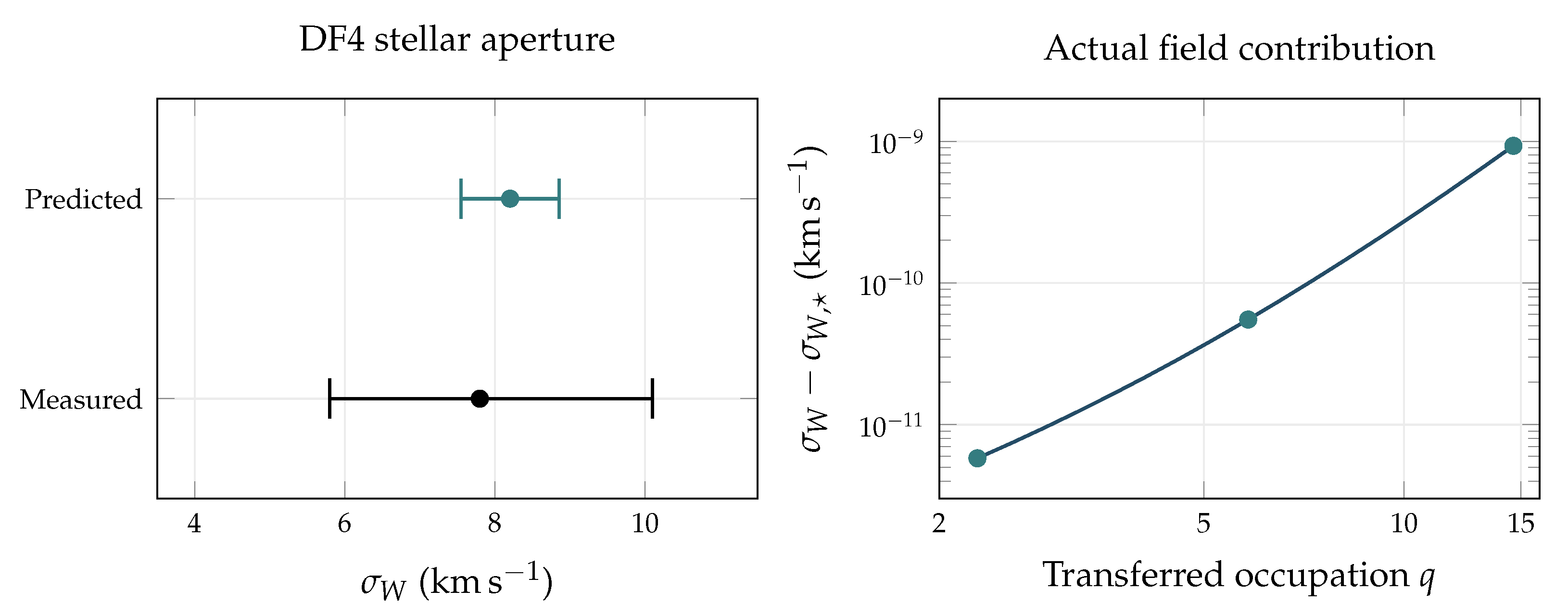
The decisive physical result is the second part of Eq. (64). The largest field contribution to the dispersion is about of the upper observational error. The agreement therefore tests the stellar-dominated limit: DF4’s measured stellar region requires no detected independent dark component, while these data cannot distinguish the transferred nonzero observation field from the zero-field solution. An agreement at this sensitivity cannot establish the field’s nonzero occupation.
10.3. Projection and Response of the Same Solution
The tiny field contribution to stellar motion follows from the radial field equation, without suppressing its coupling to gravity. To display the scale dependence, put and normalize . The same solution has
Regularity gives , and hence
The last expression applies when the light-weighted kernel lies well inside the field scale; the reported numbers use the full integral in Eq. (63). A large conserved field mass can therefore exert very little force within the stellar body when its central density is small.
Lensing projects this same density along the line of sight. A spherical shell of radius places the fraction of its mass inside a cylinder of radius R. Thus
Since the regular solution has finite central surface density,
The central sphere and cylinder masses scale differently, as and . Their difference is a projection of one source, not evidence for two gravitational components.
For an isolated lens with source and observer far outside the field, the leading asymptotic bending is . Table 8 instead reports the projected source mass itself, because the calculated field half-mass radii are – Mpc. These scales are comparable to DF4’s distance from us. Assigning the full isolated column to an observed dwarf lens would require an environmental embedding and finite-distance ray propagation. Even in a valid thin-lens limit, a nearly constant central surface density gives little tangential shear, since . The formal column prediction is therefore not a measured DF4 lensing signal.
The same stationary solution also fixes a dynamical response. Unlike the Hernquist profile used for the strong lenses, the deprojected Sérsic profile has finite global dilation inertia. Spherical symmetry gives ; integrating the projected Sérsic moments then yields
For DF4, . The canonical dilation calculation in Sect. Section 3 now applies globally within its two-coordinate family:
where and is the field gradient energy. For , the quadratic form is for every nonzero displacement. Its two variational squared frequencies are
Both are positive. The absent field coordinate is omitted at . Across the transferred interval, the faster period remains about Gyr, while the slow field-dominated period ranges from to Gyr. These are response times of the specified canonical family, not a complete mode spectrum or a measured evolutionary sequence.
This scale separation exposes the next physical requirement. The isolated ground state is a well-defined mathematical solution, but its very extended envelope and slow response do not establish that DF4 formed in that state. A connected cosmological and environmental solution must supply the boundary history and the occupation entering Eq. (60). Stellar motion, projected mass and the two-coordinate response have all been derived from one source here; only the first currently has a DF4 measurement in this comparison. The new agreement strengthens the low-source result without resolving C0302’s independent outer-motion failure or completing the observational test of a nonzero field.
11. Large-Scale Distribution in an Expanding Background
The very extended DF4 solution changes the natural boundary condition of the problem. At tens of megaparsecs, the observation field must be matched to a cosmological source and its history. Its density cannot be assigned independently to each dwarf and then integrated to infinity as if every other source were absent. We therefore continue the same quadratic branch into an expanding background and solve the coupled growth of ordinary and observation-field perturbations.
11.1. Expansion, Transport and the Common Source
Let , where is a comoving coordinate. Carrier averaging of the same covariant mode equation that gives Eq. (3) now yields
The term follows from the expanding spatial volume in the covariant wave operator. Terms beyond the weak-field, slowly varying carrier approximation are discarded, as in the galactic reduction. Putting removes the dilution term. For ordinary collisionless matter, use the specific canonical momentum and its comoving mass distribution . The common equations become
Bars denote the homogeneous densities entering the background equations. The peculiar potential is sourced by deviations from those densities. On a periodic domain its zero Fourier mode is removed; for an isolated perturbation the source is matched to the homogeneous background at large radius. This subtraction avoids counting the background gravitational effect twice.
The comoving occupation is conserved under periodic or no-flux boundaries. A homogeneous occupied field therefore has . Expansion dilutes its physical density while preserving occupation. An initially empty field still remains empty within this reduction. Structure grows from populated initial data and spatial perturbations, rather than from a change in the normalization convention.
For reference, define the peculiar kinetic and gravitational energies by
The same reciprocal source variation gives
At fixed comoving canonical data, and ; Hamiltonian evolution cancels their internal exchange and leaves this explicit scale-factor dependence. Ordinary energy conservation from the isolated calculation is consequently replaced by an expansion balance.
11.2. Growth and the Field Response Scale
To resolve the initial formation stage, write and take a cold, pressureless ordinary component on the large scales considered. This is the single-stream moment reduction of the collisionless equation. With , the real and imaginary parts of Eq. (74) give continuity and Euler equations. Linearizing them and eliminating the velocity divergences gives, for each comoving Fourier wave number k,
The fourth-order spatial term is fixed by the field gradient energy; it introduces no new coupling. Define
At , the field-gradient term equals the field’s own linear gravitational coefficient. For , the two components can grow together. For , field oscillation and gradient support suppress its response to a compact ordinary source.
This is a field-response scale, not a universal cutoff for all structure. At an instant, the gravitational growth matrix in Eq. (77), apart from the common Hubble damping, is
For and , its two eigenvalues have opposite signs. The pressureless ordinary component thus retains an attractive growth channel even where the field is strongly suppressed. In the slowly varying, short-wavelength forced limit, . A field smoothing scale cannot by itself prove that no ordinary structure can form below it.
11.3. A Solved Formation Experiment
For a definite history derived within the same branch, take a flat background, vanishing net constant source and pressureless mean densities at carrier-averaged order. The rapidly oscillating scalar pressure is averaged at this order. The homogeneous common-source equation gives , and conservation then integrates to . We set Gyr, and . These are declared initial-value experiment parameters, not an inferred expansion history of the observed Universe. The mean field fraction is likewise an input. The main calculation uses , with and used to examine the dependence on occupation. The calibrated intrinsic mass is unchanged.
Using , Eq. (77) becomes
Primes in this equation denote . Each Fourier transfer starts from equal component amplitudes and , at . The zero-wave-number solution is exactly , which supplies an independent normalization check.
We choose a smooth, compensated initial density contrast,
Here , and are comoving lengths. Both Mpc and Mpc are evolved. The integral vanishes, so the perturbation redistributes the background without changing its mean occupation. The negative compensating contrast is an underdensity; the total physical density remains positive. With the convention , the initial Fourier profile is
The specified initial derivative also fixes an irrotational velocity and field phase. At the retained perturbative order,
The spatially constant phase is arbitrary. Compensation makes at the origin, so the nonconstant phase has a regular low-wave-number limit. Occupation, spatial contrast and initial transport are therefore all specified.
If is the solved transfer, with , for either component, its radial distribution at every reported epoch follows from
Thus the spatial distribution and its formation history are outputs of one coupled initial-value solution. They are not independently chosen profiles at different times.
The declared clock gives . At and , the homogeneous field density is and the physical response wavelength is Mpc. Over the declared fraction range , that final wavelength ranges from to Mpc. These numbers describe the chosen background, rather than an observational estimate of a cosmic fraction.

Table 9.
End-time central contrasts in the coupled formation experiment. Both components start from at . The listed contrasts are departures from a positive homogeneous density.
Table 9.
End-time central contrasts in the coupled formation experiment. Both components start from at . The listed contrasts are departures from a positive homogeneous density.
| R (Mpc) | |||
|---|---|---|---|
| 1 | 0.01811428 | 0.01641958 | 0.906444 |
| 10 | 0.01968729 | 0.01968703 | 0.999986 |
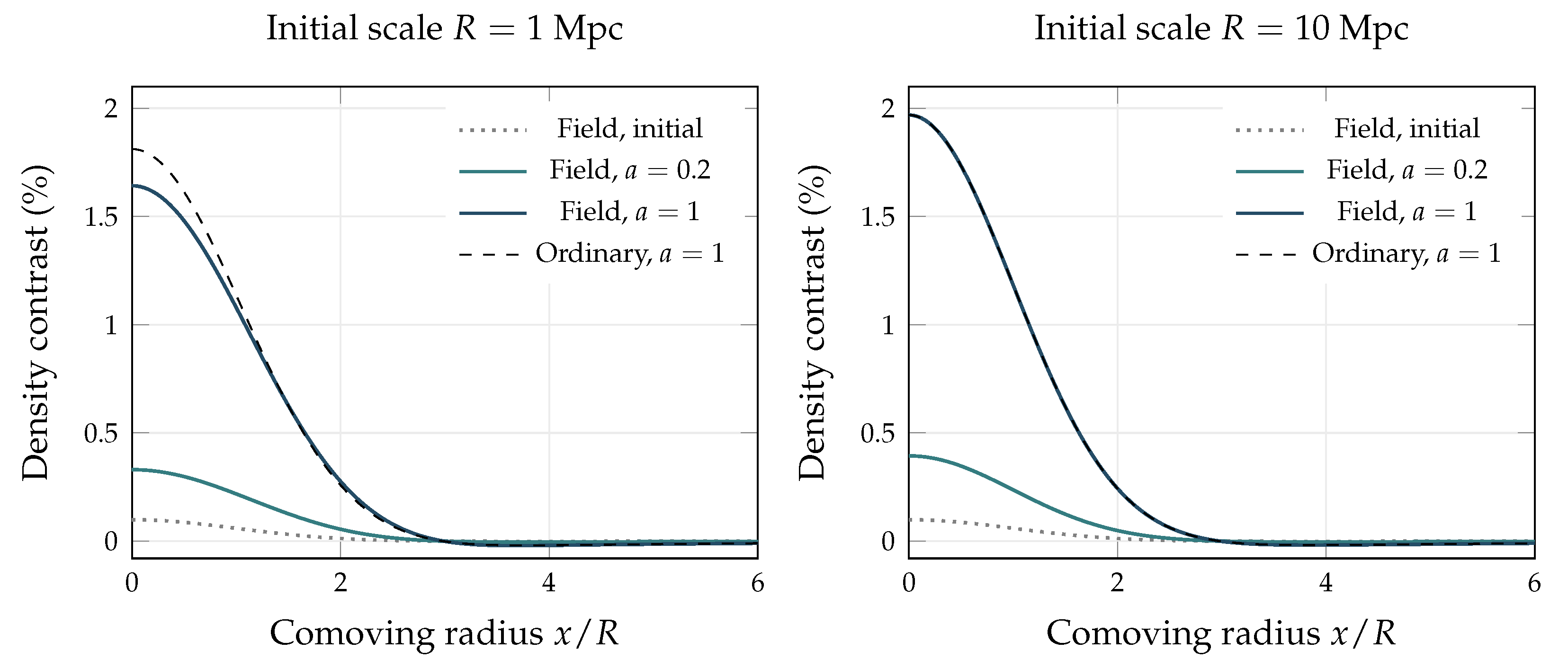
The 10 Mpc perturbation follows the common growing solution almost exactly. The 1 Mpc perturbation develops a smaller field contrast, with . This is a solved scale dependence of the same gravitational source. All recorded contrasts remain below in absolute value, so the calculation follows growth before the nonlinear collapse stage.
Figure 5.
Formation of a compensated perturbation from the coupled expanding equations at . Each curve is reconstructed from the evolving Fourier solution. On the larger scale (right), ordinary and observation-field contrasts nearly coincide; on the smaller scale (left), the field has a reduced central contrast. The negative outer contrast represents compensation relative to the positive background.
There is also a direct comparison with the isolated DF4 envelopes. Their mean field densities inside their half-mass radii, divided by the declared background field density, are , and in increasing order of the transferred occupations. If interpreted as the entire field density, each isolated envelope would lie far below this background. Interpreting it instead as a density excess requires solving for a field with a populated boundary; adding a background density to the old isolated wave profile does not solve Eq. (74). This comparison explains why the global isolated occupation cannot be read as the cosmological source mass surrounding the dwarf.
This experiment resolves the linear formation stage. Its small initial contrasts are kept within the range of the linear equations; the resulting histories are not nonlinear reconstructions of DF4’s stellar assembly. The published stellar population age, Gyr [9], supplies a useful chronological scale, but it does not specify when the observation field was populated or which spatial perturbations were present. Those initial data cannot be replaced by the stellar age.
11.4. A Stellar Probe of the Evolving Environment
The same computed distribution can be passed through the stellar and projection kernels. As a controlled probe, place the fixed DF4 stellar geometry at the centre of each evolved perturbation and calculate the extra response to its peculiar potential at . This measures the effect of the prescribed environment relative to the same background. It does not evolve the dwarf or its backreaction on that environment.
Since , the central field excess is nearly uniform throughout the stellar body. Its aperture contribution is
The reported calculation integrates the full spherical enclosed excess; the harmonic expression differs by less than in relative variance. The ordinary environmental excess is added through the same kernel, so the total peculiar variance increment is the sum of both contributions.
For a projection from that same solution, let be the evolved spherical Fourier profile. The exact infinite cylinder of the field excess is
where is the cylindrical Bessel function. At , comoving and physical lengths coincide. This follows by projecting the three-dimensional Fourier solution and integrating its transverse surface density over the aperture. The ordinary environmental column is obtained by the identical operation on its solved spectrum.
Table 10.
Passive stellar-window response to the evolved peculiar environment at . Field and total columns refer to the observation component alone and to both environmental components. Dispersion increments use the fixed stellar baseline only as their normalization. Projected masses are formal full columns of the synthetic perturbation.
| R | ||||
|---|---|---|---|---|
| (Mpc) | () | () | () | () |
| 1 | 1.06712 | 2.24437 | 12,900 | 26,563 |
| 10 | 1.27947 | 2.55896 | 143,445 | 286,892 |
The field contribution alone changes the dispersion by and for the 1 and 10 Mpc perturbations. Including the ordinary environment raises these increments to and . The corresponding field columns contain and inside the projected stellar effective radius. The larger projected response and very small local force follow from the same diffuse source and its different geometric weights.
These increments isolate the peculiar environmental source. A full physical-coordinate orbit also contains the background acceleration and the dwarf’s response to the environment. The tabulated increments therefore do not replace a complete bound galaxy solution. The infinite columns likewise require finite-distance light propagation before they become observed lensing quantities. Within the stated probe, however, distribution, gravitational response and projection have all been computed from the same evolving source.
The large-scale result sharpens the interpretation of the dwarf calculation. A real observation field can occupy the cosmological background, grow into broad structures and respond weakly inside a stellar-dominated dwarf. An isolated stationary mass and radius do not establish that background or its formation history. The connection to the measured environment requires nonlinear evolution, while preserving the same metric source for stellar motion and light propagation. We next solve a controlled nonlinear branch to follow how the profile changes as gravitational convergence becomes appreciable.
11.5. Nonlinear Growth from Specified Initial Transport
The linear solution describes how a weak contrast begins to grow. At larger amplitude, the transport itself changes the density profile: material converges toward a crest, new spatial harmonics appear, and the field gradient acts on the resulting shape. To calculate this stage, we retain the full equations of motion and choose initial data that are uniform in two comoving directions and periodic in the third. Translation symmetry preserves this reduction. It supplies a nonlinear solution of Eq. (74) on a periodic domain, with the same intrinsic mass and background used above. Its initial profile differs from the compensated spherical seed; the wavelength below is a period, not a Gaussian radius.
Let , and . Introduce
Here , and denotes the mean over one period. We impose and . For ordinary matter with a single velocity at each position, the collisionless equation closes exactly on its density and velocity until trajectories cross. The reduced equations are
The ordinary component and the field therefore respond to precisely the same potential at every step. No density profile is imposed after the initial epoch.
Both initial densities are , with . Their transport is specified by
The field canonical velocity is , so it initially equals . Substitution in the two continuity equations gives exactly, including at finite amplitude. This fixes a definite nonlinear continuation of the previously used linear initial transport. It does not assume that the finite-amplitude trajectory remains a pure growing linear mode.
The peculiar energies per unit mean comoving mass, measured in units of , are
They obey , the dimensionless form of Eq. (76). In addition, the mean ordinary mass and field occupation remain constant. These relations test the reciprocal evolution, including the work associated with expansion.
The nonlinear experiment uses , and , with the same 12 Gyr reference clock and intrinsic mass. We evolve periods and 10 Mpc from amplitudes and . A separate calculation tests the linear limit. Table 11 compares the final crest with the linear evolution of the same initial fundamental mode; Figure 6 shows the full half-period profile.
At 10 Mpc and , the ordinary and field crest contrasts reach and , respectively. The corresponding linear predictions are and . Gravitational convergence therefore produces a much narrower and higher density crest than first-order growth predicts. Although the fundamental wavelength is long compared with the field response scale, the sharpened crest contains shorter spatial harmonics. Their gradient energy makes the field crest lower than the ordinary crest by in contrast.
At 2 Mpc, the same initial amplitude gives contrasts and . The field continues to cluster, but its central contrast is only of the ordinary contrast. The difference follows from the field gradient term already present in the action. No independent short-scale smoothing prescription has been added. The histories remain smooth over the reported interval and both physical densities stay positive.
11.6. The gravitational signature of the formed profile
Reflection symmetry of these initial data preserves cosine density modes. Write the computed total contrast as . The potential, physical peculiar acceleration and its spatial derivative are then
Thus a density harmonic generates a force harmonic with one inverse power of its mode number and a potential harmonic with two. The nonlinear force is determined by the evolved source; it cannot be selected separately to improve a motion comparison. In particular, the ratio of second to first force amplitudes is .
Projection retains the same source but introduces a physical path. For a segment of physical length ℓ parallel to a uniform direction, the instantaneous excess column is
Along the periodic direction, the excess integrated over a whole period instead vanishes. This difference is a direct consequence of geometry, not a change of gravitational source. An observed lens prediction additionally requires the finite source and observer positions and propagation through the complete environment.
The calculation establishes nonlinear structure growth in a populated observation field coupled to ordinary matter. Field stress remains a real part of the source as the profile forms. Its contribution to motion, tidal acceleration and a specified column follows from one evolving solution. This supplies the next dynamical step beyond the linear experiment; a reconstruction of a particular galaxy must also determine that galaxy’s initial occupation, environment and three-dimensional formation history.
11.7. Testing the Evolved Environment against C0302
A formation calculation becomes informative for a measured galaxy when its source is passed through that galaxy’s observing geometry. C0302 provides the most demanding comparison in the present sample. Its selected source predicts an outer dispersion of , whereas the symmetric combination of the two measured outer apertures is . The central aperture measures [4]. Reaching the outer central value requires
We therefore test whether the evolved environmental source can supply the required change at the fixed stellar geometry.
The local environmental potential has the expansion
The constant term changes the carrier phase; the uniform acceleration is removed in the freely falling galaxy frame. Internal relative motion first responds to the tidal term. For the peculiar potential, . The homogeneous acceleration belongs to the background equation and is kept separate.
There is also an exact sign constraint. With stellar luminosity density and fixed anisotropy , let . The stationary radial pressure with a vanishing outer boundary term is
An added nonnegative spherical density increases and hence . Projection multiplies it by the nonnegative factor and by the nonnegative aperture response. Consequently, at fixed tracer, orbits and boundary condition,
Adding positive spherical mass cannot repair C0302’s excessive outer dispersion. An underdense environment can have the opposite sign, so its full spatial contrast must be evaluated.
For a galaxy placed at phase of the nonlinear periodic profile, write its total contrast as . Angular averaging about the galaxy centre gives its spherical monopole and enclosed excess mass:
Both the ordinary and field contrasts enter . Their separate contributions can also be propagated through the same formula. The aperture response is
where is the positive mass kernel of the retained stellar population, including the slit and seeing. We evaluate the complete profile, rather than extending a constant central tide to infinity. For the Hernquist tracer and radially increasing anisotropy, that extension would make Eq. (95) diverge logarithmically. The oscillating compensated profile has a convergent response.
We evolve the same , initial data to , corresponding to within the declared background. The published distance calibration of the stellar and lens apertures is retained. Thus the chosen expansion history supplies an experiment epoch; it is not a new distance fit. Both 2 and 10 Mpc comoving periods are evaluated over every placement phase. Table 12 gives the outer-aperture response envelope.
The largest reduction is only , compared with the required . The fixed-tracer monopole response of these environments is therefore far too small to account for the C0302 variance difference. This conclusion includes underdense placements; it does not depend on placing the galaxy at a density crest.
This computation is a signed monopole response of the fixed stellar kernel. It does not supply a new globally admissible equilibrium. Indeed, the complete periodic environment exposes a constraint on the stellar boundary. With and the retained radial anisotropy, the formal large-radius pressure becomes
For the 10 Mpc environment, the bracket reaches at both crest and trough placements. Because these wave numbers are commensurate, its negative values recur at arbitrarily large radii, where the asymptotic term dominates. A nonnegative stationary stellar distribution cannot have negative radial pressure. The isolated infinite stellar tail therefore cannot be retained unchanged in this periodic environment. The small response in Table 12 is a diagnostic of the force scale; a physical embedding must also determine the outer stellar population and its boundary condition.
11.8. The environmental mass required by the lens
A foreground or surrounding structure can contribute to the lens column while changing the stellar force by a different amount. This possibility calls for a new common-source solution, because reducing the galaxy’s assigned lens mass changes the field that supports the stars. We keep the intrinsic mode, stellar mass, scale, seeing and slit centring fixed and solve the stationary field again as its occupation ratio q changes. The existing orbital parameter remains within . The outer velocities now enter this inverse calculation explicitly.
For each recalculated source, define the equivalent missing column by
Here and kpc are the original compressed lens constraint and its aperture [4]. The quantity is an aperture budget expressed as an equivalent sheet. It is not an independently measured environmental convergence or a reconstruction of the lensed image pixels.
Table 13.
New stationary C0302 field solutions at fixed intrinsic mass, stellar source and observing geometry. The field is resolved again for every q. Velocities are in . The observed central and symmetric outer values are and , respectively. is the missing cylinder mass fraction defined in Eq. (100).
| Calculation | q | ||||
|---|---|---|---|---|---|
| Selected source | 2.2824 | 0.9033 | 259.16 | 262.82 | 0.0623 |
| Outer matched, fixed orbit | 1.1485 | 0.9033 | 210.93 | 208.78 | 0.4782 |
| Outer matched, boundary orbit | 0.9828 | 2.0000 | 216.31 | 208.78 | 0.5182 |
| Joint moment compromise | 1.3151 | 2.0000 | 228.12 | 221.89 | 0.4330 |
At the original orbital parameter, matching the outer central value requires and predicts a central dispersion of . Its lens budget requires . Continuing the outer-matching solution through the retained orbital interval raises the central prediction to a maximum of at , with . The numerical continuation does not reach both observed central values exactly.
The finite measurement errors allow a compromise. Minimizing the central and symmetric-outer squared residuals gives , , and . The normalized residuals are and ; their squared sum is . Keeping both signed outer bins gives , including the observed difference between the two sides. These are fits to the velocity summaries; their improvement does not determine the environmental column.
The compromise still requires , or . At this fixed galaxy solution and geometry, propagating the quoted lens-mass error alone gives . For comparison, an instantaneous path of physical length ℓ parallel to the planes gives the aperture-averaged environmental excess
where is the Bessel function. At a specified depth of 10 Mpc, the largest equivalent fraction from either evolved environment is , more than two hundred times smaller than the required . A 1 Mpc path gives one tenth of that column. A full period normal to the planes instead has zero excess column. These finite paths define geometric source diagnostics, with their homogeneous contribution subtracted; propagation through an actual lens environment must use its measured geometry.
Thus lowering the galaxy field can improve the velocity comparison, but the solved smooth environment does not supply the accompanying lens deficit at the tested depths. C0302 requires a different resolved source distribution or environmental structure before this common-field realization can satisfy both measurements.
The published lens fit contains shear , with a degeneracy involving the galaxy’s ellipticity and position angle. Its authors discuss nearby companions and a possible misaligned larger structure [4]. Shear constrains the traceless part of a projected potential Hessian, whereas convergence constrains its trace. The quoted shear therefore cannot be substituted for without specifying the environmental source.
The distinction between a source response and a completed embedding also matters for the observation carrier itself. A coherent field obeys
Adding two isolated density profiles does not determine the interference term or satisfy the coupled field equation. A complete environmental solution must match amplitude and phase at its boundary and evolve the resulting source together with the stars. The present calculation fixes the required motion and column scales before that matching is attempted.
12. A Spatially Resolved Test with JWST
For the early-type strong lenses studied here, the most useful next observation is a common spatial map of stellar spectra and lensed images. We select JWST NIRSpec integral-field spectroscopy together with NIRCam imaging for this purpose. The choice follows from the angular scale and tracers of these galaxies; it is not a universal ranking of telescope accuracy.
NIRSpec’s IFU covers approximately with nominal spatial elements. Its high-resolution gratings have nominal resolving power ; the G140H/F100LP setting covers approximately –m [5]. NIRCam’s short-wavelength channel samples the sky at per pixel [6]. These sampling scales permit the existing subarcsecond stellar extractions and arcsecond lens structure to be addressed in a single source model. The wavelength-dependent PSF, IFU slice response and image reconstruction still determine the effective spatial resolution.
FAST supplies a different measurement. Its measured L-band beams have half-power widths of about near GHz, and the characterized 19-beam receiver covers – GHz [7]. This is useful for sufficiently extended radio sources and sensitive neutral-hydrogen spectroscopy, but it cannot resolve the stellar absorption spectra or arcsecond lens structure required here. At the redshifts of H1417 and C0302, respectively and , the MHz hydrogen line would lie near 785 and 733 MHz, outside that particular receiver band. These conclusions concern the specified FAST receiver and the present targets.
C0302 is the decisive target because the selected common source already predicts an excessive outer dispersion. H1417 supplies a comparison where the previous orbital fit was consistent with the outer spectra. NIRSpec should measure the full line-of-sight velocity distribution across the centre and both sides of the lens, allowing and, where the spectra support it, to be inferred together. The nominal velocity resolution is
For a Gaussian line-spread function this corresponds to a dispersion of roughly . Neither number is the error on a fitted stellar dispersion. That error depends on continuum signal-to-noise, spectral templates and calibration. The proposed outer-bin goal is an uncertainty of at most , to be tested with exposure calculations and synthetic-spectrum recovery. Detector gaps must be checked for the actual absorption windows; the high-resolution IFU wavelength gaps cannot be recovered by ordinary dithering [5].
NIRCam would constrain the stellar light and extended lensed images, while the spectral cube constrains orbital structure. Their likelihoods must use the same intrinsic , with spatial PSFs, spectral response and extraction weights applied only when generating each record. Stellar population gradients and the lens environment enter as measured source uncertainties. The comparison must also retain the signed velocity information, so that rotation or spatial asymmetry can test the spherical approximation itself. Replacing that approximation, if the data require it, changes the source geometry within the common equations rather than introducing a separate lensing force.
The observational question is now precise: does one dynamically admissible observation source reproduce the light, stellar velocity distribution and lensed images simultaneously? If it does, a fit that also admits an independent component can place an aperture-defined bound on Eq. (37). If it does not, the selected observation-field realization fails that joint comparison. The present paper supplies the theoretical source and its computed response; this JWST spectroscopy experiment is a proposed test. Section 8 uses an existing published JWST distance together with Keck kinematics. No raw JWST or FAST exposure is fitted here. Target coverage and exposure requirements for the proposed strong-lens program remain to be established.
Section 11.8 makes the environmental requirement quantitative. The velocity compromise needs a substantial additional lens column, so the extended images and surrounding structure must be reconstructed together with the stellar spectra. An environmental column inferred in that reconstruction must retain its uncertainty and be compared with the field’s calculated source. The measured shear alone does not determine it. The required outer stellar boundary must also be checked against the spatial light profile, because an unchanged infinite tracer is not compatible with the periodic environment.
13. Physical Conclusions
Observation gravity is a real metric source in the tested dual-axis branch. Its energy density evolves under the observation state equation at a conserved occupation. Omitting that stress from source reconstruction places its contribution in the inferred dark residual. The source-attribution identity explains how a gravitationally inferred dark component can arise without an independent material component. It does not describe an instrumental illusion.
One action fixes the stellar force, field response and light deflection. Independent canonical dilations have a positive energy Hessian, localized displacements produce finite variational frequencies, and the direct spherical evolutions remain bounded over the reported intervals. The field and moving stars source the same potential throughout.
At DF2’s JWST distance, the measured Sérsic stellar distribution predicts through the approximated KCWI aperture, consistent with . The nonnegative extra-source fit reaches its minimum at zero. The optical measurement therefore requires no independent dark component, although the approximate profile calculation still allows 57% additional mass inside the stellar half-mass radius. This tests the low-optical-field limit admitted by the common equations.
DF4 extends the result to a target unused in the earlier calibration. With the intrinsic mode and transferred occupation interval fixed, its stellar-window prediction is , consistent with . The calculated field increases the dispersion by less than . The agreement tests the stellar-dominated limit and requires no detected independent dark component in the measured region. At this sensitivity, the nonzero transferred field and zero-field branch are indistinguishable.
The zero-residual proposition makes the exclusion criterion exact. After a correct and complete source subtraction, a zero residual excludes a nonnegative independent dark density almost everywhere in the tested region. Finite-precision data supply the bounds of Eqs. (55) and (57). The dwarf measurements support compatibility with zero additional source.
For the three measured lens cylinders, including the calibrated observation source reduces the unexplained fraction from 76.03% to a signed remainder of percentage points. These conditional aperture results use measurement-only lens errors; they do not determine a cosmological dark-component abundance.
The expanding calculation supplies an explicit initial formation stage. In the declared background, a 10 Mpc perturbation grows almost identically on both axes, whereas a 1 Mpc perturbation ends with field-to-ordinary central contrast ratio . The field gradient changes the spatial response without changing its coupling to the common potential. These are solved histories at specified occupation and initial perturbation, not an inferred cosmic abundance. Their background density also shows why DF4’s isolated 11–37 Mpc envelope cannot simply be identified with a cosmological overdensity. A nonlinear environmental solution must connect this formation stage to the measured dwarf before predicting its full line-of-sight lensing signal.
The periodic nonlinear solution establishes that the same equations also generate substantial concentration. Starting from a contrast, the 10 Mpc calculation reaches ordinary and field crest densities of and times their respective backgrounds. Their linear predictions are only and . At 2 Mpc, the field crest contrast is of the ordinary contrast. The observation field therefore grows with the source while its gradient energy limits the sharpness of the resulting structure. New density harmonics fix new force harmonics through Eq. (91); their amplitudes are outputs of the evolution. This is a concrete nonlinear formation mechanism within the selected dual-axis branch. Connecting it to a measured galaxy requires the corresponding three-dimensional initial data and environment, with the same source used for all observational records.
C0302 remains the principal unresolved galaxy comparison. Its selected source overpredicts the outer dispersion by quoted errors. A positive spherical addition cannot reduce that second moment, and the computed environmental monopole has a formal dispersion effect below . More fundamentally, the infinite isolated stellar tail is incompatible with the full 10 Mpc periodic environment: its formal radial pressure becomes negative remotely. The environmental boundary must therefore be part of the stellar solution itself.
Resolving the isolated field again while varying its occupation and retained orbital parameter improves the central and outer velocity residuals to and quoted errors. This inverse compromise requires an equivalent missing lens column fraction of , with a conditional uncertainty from the lens mass alone. The solved smooth profiles supply at most over a specified 10 Mpc physical path. The discrepancy therefore cannot be absorbed into the environment already computed here. A common-field description of C0302 must determine the stellar boundary, source geometry and phase-matched environment together, and reproduce the image and spectral records from that resulting solution. The dwarf apertures remain compatible with no independent dark component; the complete sample does not yet establish a universal exclusion.
Appendix A. Numerical Precision
The initial radial eigenstate is solved self-consistently in the analytic stellar potential, with a fixed-point tolerance of and a scale-adaptive outer boundary. The main evolution uses 1536 wave cells, stellar phase-space samples and . Q0047 and C0302 are repeated with 2048 cells, samples and . The evolution figures and tables use these refined runs where available and the main run for H1417. Each control and its disturbed partner use the same quiet stellar sequence and observing geometry. The stationary source-comparison tables recompute all three field profiles with 2048 cells and apply the same fixed aperture kernels.
Sampling the full is important for this experiment. Independent initial-state comparisons at samples give a maximum radial velocity-dispersion error of across eight equal-mass bins, a maximum slit-dispersion error of , and a maximum projected fourth-moment error of in the representative sampling test. The radius follows the exact untruncated stellar cumulative law. The velocity construction numerically inverts the positive augmented-density Abel transform in the same potential.
The empirical stellar energy omits the diagonal term. If it were included, a finite shell would acquire the artificial self acceleration even when the continuous stellar density has finite central acceleration. The omitted mean energy is only in the adopted stellar units, since its initial density gives . The correction therefore vanishes with sample size, while avoiding a nonuniform central self-force error. Star–field interactions remain reciprocal and retain every stellar mass in the lensing and wave source.
In the reported trajectories, the largest relative total-energy error is , the largest field-norm error is , and the largest end-point relative specific-angular-momentum error is . The energy error is also compared with the much smaller injected perturbation energy; its largest ratio is 0.032%. The largest coarse-to-refined difference in the paired dispersion response is 1.40 , and the corresponding cylinder-mass difference is 0.0106 of a quoted lens-mass error. These comparisons concern the numerical response of the selected states; they are not additional observational uncertainties or a posterior stability probability.
The localized energy Hessians are computed with 2000 field cells and compared with 1000-cell solutions. The largest period change across all three galaxies and three trial scales is . For C0302 at , centered finite differences of the exact finite-deformation energy agree with the analytic Hessian to relative at displacement step and at step . The separate component virial identities provide an additional comparison with the global positive-curvature matrix.
The accompanying source includes the selected initial states, their calibration provenance, the positive phase-space sampler, the reciprocal Hamiltonian solver, all reported trajectory records, the Hessian calculation and the vector figure data. The final LaTeX file is standalone and compiles without external figure or bibliography files. The monograph version defining the branch and normalization is included in the source record. Instrument documentation is used to design the proposed JWST test; the numerical evolution uses the existing HST and Keck constraints and introduces no external dark-sector mechanism.
Appendix A.1. DF2 Deprojection and the Extended Field
The Sérsic density is integrated through its exact Abel transform on 3001 logarithmic radial nodes, using 180 Gaussian nodes for the regularized deprojection integral. Before normalization its integrated mass differs from unity by . The field uses an adaptive boundary-value solution of the radial wave equation, Poisson equation and normalization equation. A regular central potential derivative is imposed, and is integrated directly. Thus the small-radius mass obeys even when the field extends far beyond the stellar body.
The main field residual tolerance is , with a refined upper-contour solution at . Increasing the light and aperture quadratures and refining the field changes the reported upper-contour dispersion by less than and its spherical fraction by less than . These numerical differences are negligible beside the observational and structural uncertainties. An independent integration of Jeans pressure followed by aperture projection agrees with the cumulative-mass kernel to relative . Analytic differentiation of the Abel integrand checks the sufficient phase-space condition at 701 radii from to for five field amplitudes; the endpoint asymptotics have positive signs. This is a numerical admissibility check with controlled endpoints, rather than an interval proof on every radius.
The DF2 source package includes the versioned observational inputs, the figure-derived aperture coordinates, all computed field-response records, the approximate profile statistic and its independent phase-space verifier. The theoretical source is monograph version 29, whose source-determination extension preserves the common-action quadratic equations used for the preceding evolution calculations.
Appendix A.2. DF4 Prediction and Response
The DF4 forward calculation reads the photometry, observing geometry and fixed transfer rule; the velocity summary is read by a separate comparison script after the field solutions have been computed. The accompanying records contain the three historical occupations, the intervening grid and the source versions. This separation prevents fitting the target velocity in the forward calculation; it does not make the retrospective target selection blind.
The nominal exact-Abel and field quadratures use the DF2 solver with . Increasing the stellar radial grid from 3001 to 6001 nodes, the Abel quadrature from 180 to 260 nodes and the aperture quadratures, while solving the field at residual tolerance , changes the predicted dispersion by or less. The direct field contrast is evaluated from its positive variance integral, using
This avoids subtracting two nearly equal dispersions. Its relative change under refinement is . These computational precisions describe the integrals, not the accuracy of the physical prediction. An independent integration of Jeans pressure followed by aperture projection agrees with the cumulative-mass kernel to relative .
Analytic Abel derivatives give a positive sufficient Eddington bracket at all 301 sampled radii between and for and the upper transferred occupation, with positive endpoint asymptotics. This is a numerical admissibility check, not a continuum interval proof. The analytic Sérsic inertia in Eq. (70) agrees with independent radial integration to relative . The positive generalized Hessian eigenvalues are computed from , avoiding cancellation in the smaller root of Eq. (72).
The radial coordinate scale used by the boundary-value solver is chosen for numerical conditioning; it is not a theoretical core-size law. All radii, projected masses and response coefficients are integrated from the solved normalized eigenfunction. The projected DF4 columns and slow periods retain the isolated boundary assumption and must be re-evaluated in a finite-distance environmental model before comparison with a lens measurement or a formation history.
Appendix A.3. Expanding-Field Formation
The linear common-source system is integrated in with an adaptive eighth-order Runge–Kutta method. The reference calculation uses relative tolerance and absolute tolerance , 401 wave-number nodes and . A second calculation uses tolerances and , 1001 nodes and . The largest difference in reconstructed profiles is in absolute contrast, or of the reference growing amplitude.
The transfer reproduces to relative or better. This zero mode is an analytic normalization check; the compensated seed itself has no homogeneous perturbation. The initial Fourier inversion reproduces the analytic radial profile to absolute . The exact zero total contrast follows from the vanishing initial Fourier zero mode and its homogeneous evolution. The finite radial windows, ending at , leave a signed-to-absolute contrast-volume ratio below .
At the starting epoch, , consistent with the slowly varying carrier reduction. The physical interpretation is restricted to weak, subhorizon perturbations. The largest density contrast is ; omitted nonlinear terms begin at second order in contrast. The integration tolerances therefore measure numerical precision within the linear model, not the error of a nonlinear galaxy-formation prediction. The source archive includes the complete radial profiles, time samples, Fourier transfers and background assumptions, with no observational likelihood entering the formation integration.
The passive stellar probe integrates enclosed density excess directly from the evolved spectrum and compares it with the local harmonic expansion. Its leading curvature correction accounts for the relative variance difference to the reported precision. Independent real-space and spectral central-column integrations agree within . The underlying density remains positive despite the negative compensating contrast. These checks concern projection of the specified linear environment; they do not test a nonlinear embedded galaxy.
Appendix A.4. Nonlinear Periodic Evolution
The nonlinear calculation uses Fourier differentiation and Poisson inversion on a uniform periodic grid. Each step composes a half common-potential kick, a full kinetic drift and a second half kick with the recomputed source. For endpoints , the integrated coefficients are
A gravity half kick changes u by and multiplies by . The wave kinetic drift multiplies Fourier mode n by . The ordinary drift solves and with fourth-order Runge–Kutta steps and a cutoff on nonlinear product derivatives, where is the grid size. The force applied to the ordinary velocity is projected onto the same retained fluid modes. The complete composition is second order in . No density clipping or field renormalization is applied.
The cold ordinary subsystem also admits an exact finite-amplitude comparison when . Let label the initial Eulerian position, and . Define
In mass coordinates, plane Poisson integration gives , so the characteristic equation integrates to
This formula is valid while the denominator is positive. It tests nonlinear ordinary transport independently of the wave solver and of the linear perturbation equations. The coupled runs retain both components and are compared separately with the linear system at small amplitude.
The reported coupled trajectories use 512 grid points and 6000 uniform steps in from to zero. Doubling the step count, and then doubling the grid at the refined step count, for the runs at both wavelengths changes the final ordinary density by at most and the field density by , in units of their respective mean densities. The fundamental amplitudes agree with an independently integrated linear system to relative or better. The exact finite-amplitude solution agrees with the numerical ordinary density to absolute and its canonical velocity to at .
Across the six main trajectories, the maximum ordinary mass drift is and the field occupation drift is . Define
Dividing its magnitude by gives a maximum of , decreasing to in the refined finite-amplitude trajectories. The integral uses endpoint trapezoidal quadrature at every time step.
The resolved characteristic relation gives a numerical Jacobian lower estimate of from the sampled maximum density over these trajectories. The converged profiles remain smooth and are consistent with a single-stream cold flow. The largest is and the largest ordinary speed is , consistent with the weak-field and nonrelativistic reduction. This calculation reaches substantial nonlinear contrast while resolving the approach to concentration before trajectory crossing.
Appendix A.5. C0302 Environment and Inverse Source
The environmental evolution uses the preceding periodic solver with its terminal logarithmic epoch changed to . The initial occupation, contrast and phase prescription are unchanged. The primary runs use 512 points and 6000 steps, and the comparison uses 1024 points and 12000 steps. The stellar aperture kernel is sampled at 3201 logarithmic radii from to ; its radial refinement uses 6401 points. The low-argument part of Eq. (97) is evaluated with spherical Bessel functions to avoid cancellation. The remaining sine and cosine integrals are evaluated separately by oscillatory quadrature in radial intervals. Their large-radius contribution is bounded using the asymptote of the aperture kernel.
The combined evolution and projection refinement changes the response by at most over placement phase. For the retained Fourier series, phase extrema follow from the roots of the derivative of its Chebyshev polynomial in ; the sum of absolute harmonic coefficients gives a separate all-phase bound. The omitted density coefficients and quadrature estimates are retained with the computed mode responses. The pressure tail of Eq. (99) is evaluated separately: its negative recurrent coefficient in the 10 Mpc case establishes failure of a globally nonnegative radial pressure for the unchanged infinite tracer. The aperture integral is consequently reported as a formal force-response diagnostic, not a new stationary stellar model.
The inverse calculation resolves the radial observation field for every trial occupation. A continuation over 42 orbital values, including the original value and both endpoints, is followed by bounded scalar searches for the extrema and the least-squares compromise. The base, refined and final field meshes contain 1500, 3000 and 6000 cells. The final aperture integration uses 7201 radial, 260 polar, 2601 sky-radius and 320 azimuthal nodes, with 512 lens-projection nodes.
From the refined to final solutions, the refitted central dispersions change by less than and the missing sheet fractions by less than . An independent integration of the radial pressure agrees with the cumulative-mass aperture kernel to relative in variance. Direct re-solution of the original selected field gives , compared with the earlier projection. This difference is numerical refinement and is negligible beside the measured outer error; it is not an environmental correction.
The two signed outer measurements retain their separate residuals. For a symmetric prediction s, their diagonal-error sum is exactly
The final constant is . The diagonal error treatment follows the earlier calculation; no unreported covariance is introduced. The inverse source results, conditional outer-error sensitivities, field profiles and finite-path environmental responses are all included in the reproducible source package.
References
- X. Meng, Physical–Observation Cosmology, Cosmological Source and Evolution Edition. Author’s monograph manuscript, September 2026, source version 29.
- X. Meng. A Phase-Space Test of a Common Formation Field: Radial Orbits, Strong Lensing, and Fourth Velocity Moments Companion manuscript. 2026. [CrossRef]
- Koopmans, L. V. E.; Treu, T. The structure and dynamics of luminous and dark matter in the early-type lens galaxy of 0047–281 at z=0.485. Astrophys. J. 2003, 583, 606–615. Available online: https://arxiv.org/abs/astro-ph/0205281, version 2. [CrossRef]
- Treu, T.; Koopmans, L. V. E. Massive dark-matter halos and evolution of early-type galaxies to z≈1. Astrophys. J. 2004, 611, 739–760. Available online: https://arxiv.org/abs/astro-ph/0401373, version 2. [CrossRef]
- Space Telescope Science Institute, NIRSpec IFU Spectroscopy. JWST User Documentation. Available online: https://jwst-docs.stsci.edu/jwst-near-infrared-spectrograph/nirspec-observing-modes/nirspec-ifu-spectroscopy (accessed on 10 September 2026).
- Space Telescope Science Institute, NIRCam Detector Overview. JWST User Documentation. Available online: https://jwst-docs.stsci.edu/jwst-near-infrared-camera/nircam-instrumentation/nircam-detector-overview (accessed on 10 September 2026).
- Jiang, P.; et al. The fundamental performance of FAST with 19-beam receiver at L band. Res. Astron. Astrophys. 2020, 20, 064. Available online: https://arxiv.org/abs/2002.01786. [CrossRef]
- Tang, Y.; Anand, G. S.; Romanowsky, A. J.; van Dokkum, P. G.; Bundy, K. A. New Measurements of Distances to Galaxies in the NGC 1052 Field with the Hubble and James Webb Space Telescopes: Testing the Bullet-Dwarf Origin of the Trail (2026). 22 June 2026. Available online: https://arxiv.org/abs/2606.05144v2.
- Tang, Y.; et al. Testing the Bullet Dwarf Collision Scenario in the NGC 1052 Group Through Morphologies and Stellar Populations. Astrophys. J. 978 2025, 21. Available online: https://arxiv.org/abs/2410.19331v1.
- Danieli, S.; van Dokkum, P.; Conroy, C.; Abraham, R.; Romanowsky, A. J. Still Missing Dark Matter: KCWI High-Resolution Stellar Kinematics of NGC 1052-DF2. Astrophys. J. Lett. 2019, 874, L12. Available online: https://arxiv.org/abs/1901.03711v2. [CrossRef]
- Keim, M. A.; van Dokkum, P.; Shen, Z.; Danieli, S.; Pasha, I. A Third Galaxy Missing Dark Matter along a Trail of Galaxies in the NGC 1052 Field (2026). 15 June 2026. Available online: https://arxiv.org/abs/2603.15860v2.
- X. Meng, Physical–Observation Cosmology, Internal Source Determination Edition. Author’s monograph manuscript, September 2026, source version 31
- Danieli, S.; et al. A Tip of the Red Giant Branch Distance to the Dark Matter Deficient Galaxy NGC1052-DF4 from Deep Hubble Space Telescope Data (2020). Available online: https://arxiv.org/abs/1910.07529v3. [CrossRef]
- Shen, Z.; van Dokkum, P.; Danieli, S. Confirmation of an anomalously low dark matter content for the galaxy NGC1052-DF4 from deep, high resolution continuum spectroscopy (2023). Available online: https://arxiv.org/abs/2309.08592v2.
| 1 | The arXiv abstract-page metadata instead lists ; the article PDF gives the asymmetric posterior summary quoted here. |
Figure 1.
Paired response of the formation-field and stellar half-mass radii. Only the field is dilated initially; the stellar response develops through the common potential. These are simulated trajectories for selected states, not observed temporal variations. The computed displacements remain bounded over the displayed intervals.
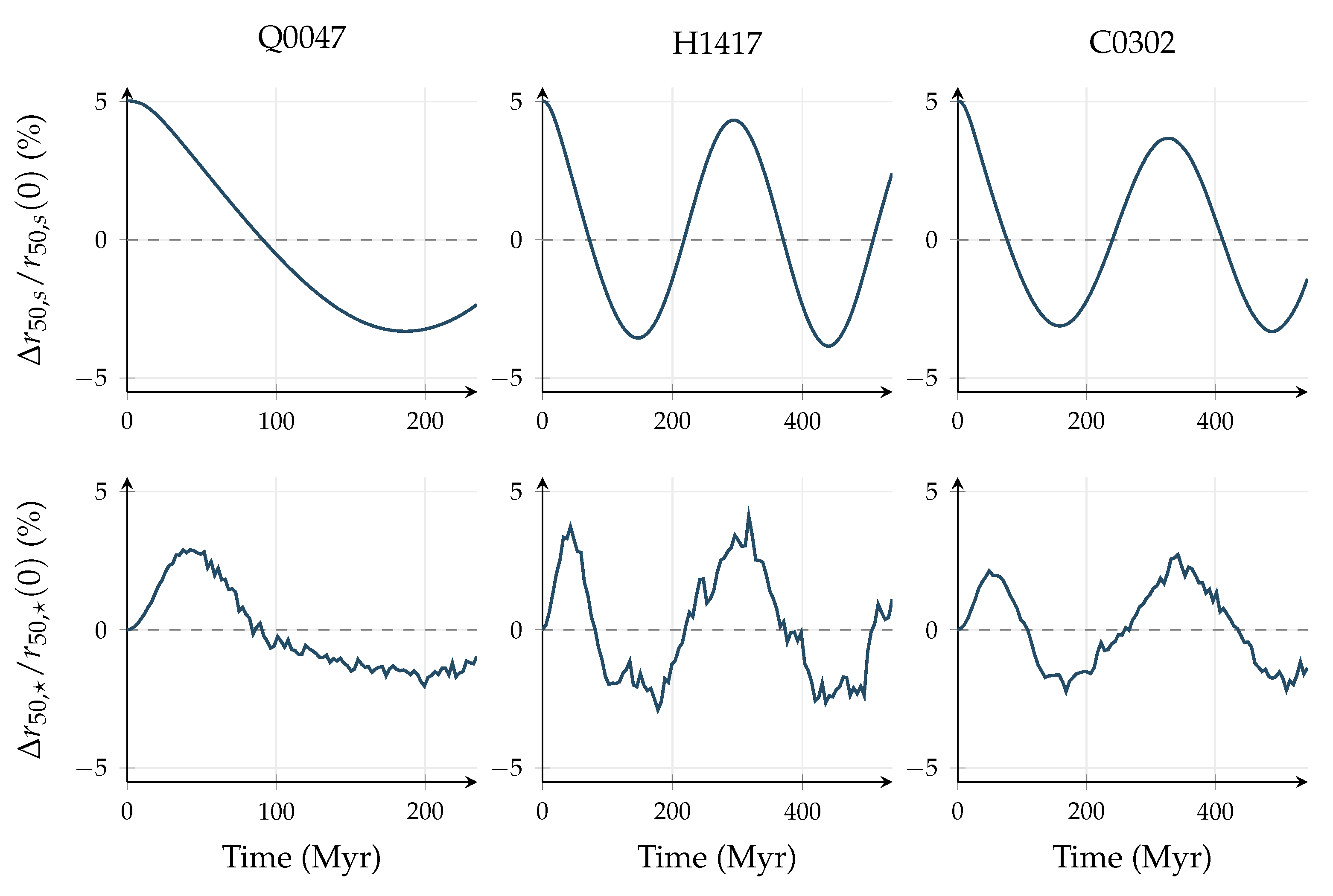
Figure 2.
C0302 motion and lensing from the same disturbed trajectory. Gray bands show the published outer weighted mean and lens mass with one quoted standard deviation, displayed as reference constraints rather than observed time series. The lens mass oscillates near its calibration range while the outer dispersion stays well above its observed mean.
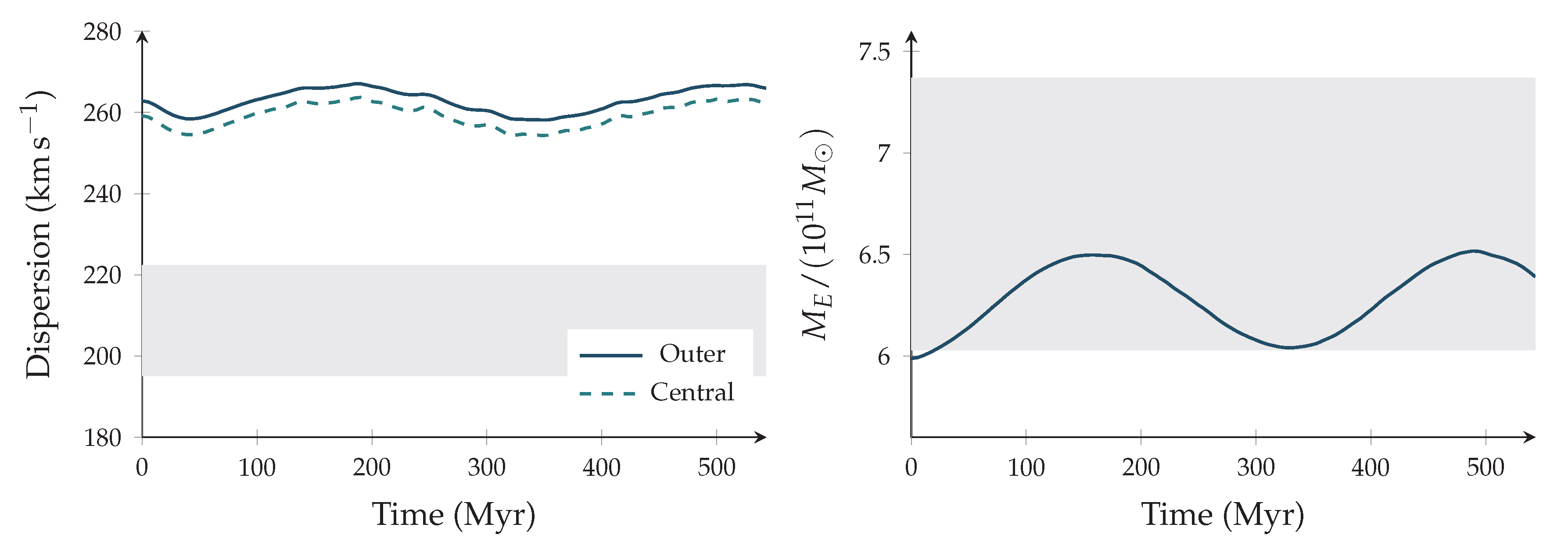
Figure 6.
The evolved half-period at for the exact initial transport of Eq. (89), with . The crest is at and the trough at ; reflection gives the other half of the period. The smooth nonlinear profiles include all resolved harmonics, whereas each linear curve contains only the initial fundamental. Both panels use the same intrinsic field mass and mean fraction.
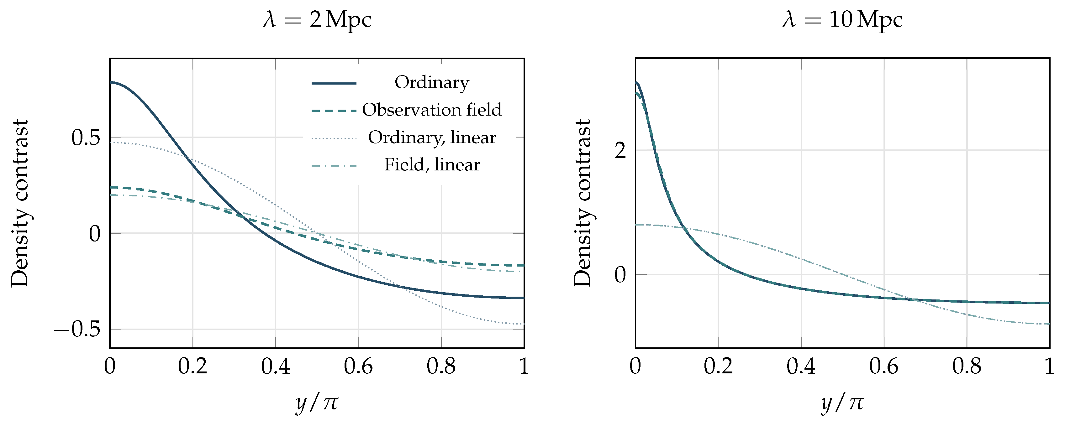
Table 1.
Selected stationary states. The common intrinsic mass is ; . The final column is the physical time covered by .
Table 1.
Selected stationary states. The common intrinsic mass is ; . The final column is the physical time covered by .
| Object | b (kpc) | q | Time (Myr) | |||
|---|---|---|---|---|---|---|
| Q0047 | 2.210 | 3.246 | 5.832 | 0.681 | 11.777 | 234.7 |
| H1417 | 1.185 | 4.585 | 14.613 | 0.949 | 15.544 | 537.9 |
| C0302 | 5.261 | 7.584 | 2.282 | 0.903 | 2.117 | 543.1 |
Table 2.
Two-component variational periods in Myr for the declared localization scale. Both periods are real; they are response frequencies of the two-shape restriction, not the complete kinetic spectrum.
Table 2.
Two-component variational periods in Myr for the declared localization scale. Both periods are real; they are response frequencies of the two-shape restriction, not the complete kinetic spectrum.
| Object | |||
|---|---|---|---|
| Q0047 | |||
| H1417 | |||
| C0302 |
Table 3.
Largest absolute response to a 5% field dilation relative to the paired control during . Radius and cylinder changes are percentages of the initial control values; dispersion changes are in . For Q0047 the outermost folded bin is used.
Table 3.
Largest absolute response to a 5% field dilation relative to the paired control during . Radius and cylinder changes are percentages of the initial control values; dispersion changes are in . For Q0047 the outermost folded bin is used.
| Object | (%) | (%) | (%) | |
|---|---|---|---|---|
| Q0047 | 5.02 | 3.14 | 5.45 | 3.64 |
| H1417 | 5.03 | 4.12 | 6.33 | 7.25 |
| C0302 | 5.02 | 2.72 | 4.71 | 5.22 |
Table 4.
Lens cylinder mass with the stellar source alone and after adding the calibrated observation source. Masses are in . The observation fraction refers to the model cylinder, not the global mass budget.
Table 4.
Lens cylinder mass with the stellar source alone and after adding the calibrated observation source. Masses are in . The observation fraction refers to the model cylinder, not the global mass budget.
| Galaxy | Stars | Observation | Sum | Measured | Observation (%) |
|---|---|---|---|---|---|
| Q0047 | 1.34 | 2.83 | 4.17 | 67.9 | |
| H1417 | 0.70 | 7.02 | 7.71 | 91.0 | |
| C0302 | 2.24 | 4.04 | 6.28 | 64.3 |
Table 5.
Outer stationary dispersion in for the controlled source comparison. The last column is the observation source contribution to , not to . Both target outer measurements are retained through their weighted mean.
Table 5.
Outer stationary dispersion in for the controlled source comparison. The last column is the observation source contribution to , not to . Both target outer measurements are retained through their weighted mean.
| Galaxy | Stars alone | Common source | Measured | Observation in (%) |
|---|---|---|---|---|
| Q0047 | 124.7 | 204.1 | 62.7 | |
| H1417 | 105.3 | 231.3 | 79.3 | |
| C0302 | 179.9 | 262.8 | 53.2 |
Table 6.
DF2 under the same intrinsic observation mode, at the central JWST distance and stellar normalization. is the spherical observation-source fraction at kpc; is the field’s global half-mass radius. Global q is not an optical mass fraction. The last finite-limit row uses with the stellar source held fixed.
| q | () | (%) | (kpc) |
|---|---|---|---|
| 0 | 7.766 | 0.00 | — |
| 15 | 7.766 | 11345.32 | |
| 1000 | 7.778 | 0.31 | 203.03 |
| 3000 | 8.689 | 20.03 | 67.81 |
| 4467.4 | 11.610 | 55.12 | 45.55 |
| 10000 | 43.613 | 96.83 | 20.36 |
Table 7.
Unexplained fractions of the measured lens-cylinder mass, before and after including the calibrated observation source. The errors are measurement-only, at fixed model parameters. The pooled row weights by the measured cylinder masses and assumes independent reported mass errors. It excludes DF2 and is not a cosmic mass budget.
| Object | Before (%) | After (%) | Mass residual |
|---|---|---|---|
| Q0047 | 66.99 | -0.56 | |
| H1417 | 90.18 | -0.83 | |
| C0302 | 66.56 | +0.62 | |
| Pooled | 76.03 | -0.32 |
Table 8.
DF4 source and response at three transferred occupations. All columns follow from the same isolated field solution. The sphere uses the stellar three-dimensional half-mass radius; the cylinder uses the projected effective radius. is the slow variational period. The Mpc-scale columns and periods are formal isolated forecasts.
| q | ||||
|---|---|---|---|---|
| (Mpc) | () | () | (Gyr) | |
| 2.28236 | 37.10 | 1.01 | ||
| 5.83232 | 22.09 | 6.72 | ||
| 14.61336 | 11.05 | 63.87 |
Table 11.
Nonlinear formation at . Contrasts are relative to each component’s own homogeneous density; its physical density ratio at a crest is . The last column is the ratio of the second to first harmonic of the total peculiar force. These are initial-value calculations, not measured galaxy profiles.
| (Mpc) | ||||||
|---|---|---|---|---|---|---|
| 2 | 0.02 | 0.236 | 0.099 | 0.295 | 0.109 | 0.083 |
| 2 | 0.04 | 0.472 | 0.199 | 0.785 | 0.239 | 0.162 |
| 10 | 0.02 | 0.400 | 0.399 | 0.635 | 0.633 | 0.180 |
| 10 | 0.04 | 0.799 | 0.798 | 3.089 | 2.918 | 0.330 |
Table 12.
C0302 response to the solved nonlinear environments. The velocity columns express the signed monopole response as an equivalent change in the reference outer dispersion, in , over the full placement phase. The final column is the maximum equivalent excess sheet fraction for a specified 10 Mpc physical path parallel to the planes, averaged inside the lens aperture. All columns include ordinary and field excess density relative to the same background.
| (Mpc) | Minimum | Maximum | Maximum |
|---|---|---|---|
| 2 | -0.001453 | 0.001919 | |
| 10 | -0.005066 | 0.009213 |
Disclaimer/Publisher’s Note: The statements, opinions and data contained in all publications are solely those of the individual author(s) and contributor(s) and not of MDPI and/or the editor(s). MDPI and/or the editor(s) disclaim responsibility for any injury to people or property resulting from any ideas, methods, instructions or products referred to in the content. |
© 2026 by the authors. Licensee MDPI, Basel, Switzerland. This article is an open access article distributed under the terms and conditions of the Creative Commons Attribution (CC BY) license (http://creativecommons.org/licenses/by/4.0/).
Copyright: This open access article is published under a Creative Commons CC BY 4.0 license, which permit the free download, distribution, and reuse, provided that the author and preprint are cited in any reuse.