

Submitted:
10 September 2026
Posted:
11 September 2026
You are already at the latest version
Abstract
Scanning precession electron diffraction in transmission electron microscopy (TEM-SPED) enables highly accurate nanoscale orientation mapping and facilitates time-resolved tracking of microstructural changes, including grain boundary migration in polycrystalline metallic materials during isothermal or isochronal heat treatments. However, achieving full predicting grain boundary migration behavior requires further advances, including the integration of experimental observations with computational simulations. In this study, we addressed this challenge by directly assimilating TEM-SPED orientation maps into a multiphase-field model using an ensemble Kalman filter, wherein simulation parameters were iteratively updated to reproduce the experimental observations. The same field of view in a 50% cold-rolled pure-aluminum foil was repeatedly observed by TEM-SPED after successive ex situ isothermal annealing at 400 °C for up to 20 min at 5 min intervals. Through the assimilation process, grain boundary mobilities that reproduced the experimentally observed microstructural evolution were identified. A simulation restarted from the initial microstructure using the inferred mobilities achieved approximately 91% agreement with the experimental observations, suggesting that the inferred mobilities were suitable for predicting the observed microstructural evolution. These results demonstrate that the direct assimilation of nanoscale TEM-SPED observations improves the prediction of complex local grain boundary migration and enables the estimation of effective grain boundary mobilities.
Keywords:
data assimilation
; ensemble Kalman filter
; multiphase-field model
; grain-boundary mobility
; scanning precession electron diffraction
; transmission electron microscopy
; recrystallization
; grain growth
; pure aluminum
1. Introduction
The microstructure of metallic materials strongly influences their mechanical properties, including strength, formability and mechanical anisotropy [1]. Heat treatment is one of the most widely used methods for controlling these properties through tuning microstructural characteristics, such as grain size distribution. The approach has been applied not only to metallic materials processed through conventional manufacturing routes but also to materials produced by advanced techniques, including laser powder bed fusion, which often generates heterogeneous as-built microstructures [2]. To design efficient heat-treatment process, both microstructure characterization and rational simulation are crucial.
Scanning precession electron diffraction (SPED) in transmission electron microscopy (TEM) is well suited to observe the microstructure at the nanometer scale. In SPED, the incident electron beam is precessed around the optic axis at a fixed angle during acquisition. As a result, the recorded diffraction pattern represents an integration over a range of beam incidence directions, substantially reducing dynamical diffraction effects and yielding diffraction patterns that are closer to the kinematical condition [3,4]. Therefore, crystal orientation can be determined at each sampling position by template matching of diffraction spot patterns rather than of Kikuchi bands. This approach enables reliable orientation indexing even in heavily deformed materials [5,6]. Because the measurement is non-destructive, the same area can be re-measured after successive annealing, producing a time-resolved record of boundary migration at the nanoscale.
For predicting the boundary migration during heat treatment it is more effective to integrate the observation results with computational methods than to rely solely on the observation. Multiphase-field (MPF) modeling is widely used to predict microstructural evolution during heat treatment, including dynamic and static recrystallization as well as grain growth [7,8,9,10]. In MPF models, the microstructure is represented by continuous order parameters, allowing topological changes such as grain shrinkage and disappearance to be handled without explicitly tracking the interfaces [9,11]. However, some input parameters are difficult to determine experimentally. For example, the grain boundary mobility, which governs the rate of grain boundary migration in MPF simulations, depends predominantly on temperature and the character of individual grain boundaries [1,12]. Identifying all grain boundary mobilities within an observed area under a given experimental condition is not always possible. Therefore, a rational and practical method for estimating these parameters from experimental observation is required.
Data assimilation (DA) techniques provide an effective method by connecting observation results and simulations. One of the data assimilation techniques, ensemble Kalman filter (EnKF) [13,14], approximates the probability density function of the system state using a finite ensemble, and is therefore applicable to high-dimensional nonlinear systems. This method has been applied to phase-field simulations of grain growth, where anisotropic grain boundary properties were inferred in synthetic microstructure models [15,16]. The other method, Bayesian data assimilation based on an ensemble square root filter, has also been coupled to an MPF model and in situ SEM-EBSD observation of static recrystallization in an aluminum alloy, to estimate the stored-energy distribution of the deformed texture [10]. Although SEM-EBSD records back scattered signals from the specimen surface, the observed surface is influenced not only by the grains at surface but also by the grains beneath the surface. TEM-SPED, on the other hand, records nanoscale electron diffraction patterns from electron-transparent specimens. In most cases, grains do not overlap along the beam direction. Therefore, heat treatment behavior observed by TEM-SPED is likely governed by interactions among visible grains. Considering that TEM-SPED can acquire crystal orientation at the nanoscale, incorporating TEM-SPED data into MPF models would be effective for accurately estimating heat treatment behavior. However, data assimilation methods for SPED have not yet been established.
In this study, we performed data assimilation using SPED datasets and discussed the accuracy of inferred parameters. The same field of view in a 50 % cold-rolled pure aluminum was characterized by TEM-SPED before annealing and after four successive 5min heat treatments at 400 °C. The resulting grain-label maps were assimilated into a multiphase-field model ensemble Kalman filter. Grain boundary mobilities to reproduce the experimentally observed microstructural evolution were subsequently evaluated.
2. Materials and Methods
2.1. Specimen Preparation
A 50 % cold rolled pure aluminum (A1050, Al ≥ 99.5 wt.%) was used as a specimen. Deformation of this magnitude introduces high dislocation density, whose redundant elastic strain energy is released on subsequent annealing [1]. The grain boundary migration observed in this study was therefore driven principally by the stored strain energy.
The specimen was mechanically polished to the thickness of less than 0.1 mm. A disc punch (Gatan, Inc.) was used to obtain a disc specimen with 3 mm in diameter. The specimen was subsequently thinned by twin-jet electropolishing (E.A. Fischione Instruments, Inc.) in a 3:7 mixture of HNO3 and CH3OH at −30 °C, 25 V and 40 mA. A reference mark was made on the rim of disk to identify the rolling direction when the specimen was loaded onto a TEM holder. The polished disc is shown in Figure 1(a) and the summary of specimen preparation conditions is listed in Table 1.
2.2. Ex Situ Annealing and Relocation of the Same Field of View
The specimen was observed and heated ex situ, so that every measurement was made at room temperature under stable conditions. The heating was performed using a tubular electric furnace (Asahi Rika Manufacturing Co., Ltd.) at 400 °C for 5 min under an argon atmosphere, followed by air cooling; the 5 min was measured from insertion of the specimen into the pre-heated furnace. The cycle was repeated until cumulative annealing times of 5, 10, 15 and 20 min were reached - five orientation maps were obtained at 0, 5, 10, 15 and 20 min.
Because the specimen was removed from the holder at each step, positional and rotational offsets were unavoidable. To align the region of interest throughout the repeated processing steps, the hole created during electropolishing was used as a fiducial marker for fine translational and rotational correction, as shown in Figure 1(b). The hole maintained a consistent shape throughout the series of measurements, indicating the absence of significant oxidation around it.
2.3. TEM-SPED Acquisition and Orientation Analysis
TEM observation was performed using JEM-ARM200F (JEOL) operated at 200 kV with a double-tilt holder. Electron diffraction patterns were acquired by SPED, over a 5.4 × 5.4 µm area with a step size of 20 nm (270 × 270 points) and a precession angle of 0.5°, using the TopSpin acquisition software (NanoMegas). TEM images of the region of interest were recorded at each step.
Crystal orientation was determined by template matching [5,6] using DiffGen and Index (NanoMegas). Simulated diffraction patterns were generated for the face-centered-cubic aluminum structure an acceleration voltage of at 200 kV on a 1° orientation grid. Image processing incorporated in the Index was performed to the recorded electron diffraction patterns before the template matching, including diffraction pattern centering and camera length calibration, noise reduction and diffraction spot enhancement to maximize the degree of match with the simulated diffraction patterns.
To assign crystal orientations as phase-field variables, the crystal orientations were grouped based on a tolerance of ±2.5° for each component of the Euler angle. Lattice distortion from dislocations perturbs the recorded electron diffraction patterns relative to the simulated ones [5,6], producing isolated mis-indexed points within grain interiors and near grain boundaries. These points were inspected individually by using their electron diffraction patterns and assigned to the adjacent grain (Figure S1), thereby removing indexing artifacts that would otherwise have entered the assimilation as spurious observations.
2.4. Region of Interest and Phase-Field Initialization
A 30 × 30-point square region of interest (ROI), corresponding to an area of 600 × 600 nm2 and located 1.45 µm from the edge of the hole, was extracted from the full map as indicated in Figure 2(a). The extracted region contained four groups of orientations, and therefore, four phase-field variables (φ1 – φ4) were defined as shown in Figure 2(b). The grain boundary migration proceeded as the heat treatment continued. No nucleation or abnormal grain growth occurred during this study.
3. Numerical Model and Data Assimilation
3.1. Multiphase-Field Model
The microstructure of the region of interest was described by four non-conserved phase-field variables φi(r, t), where i = 1, …, N with N = 4 identifies the grain, r = (x, y) is a point on the 30 × 30 square grid of spacing Δx = Δy = 20 nm, and t is time. φi equals unity inside grain i and zero outside it, and varies smoothly across a diffuse interface of finite width δ, which in this study was set to 7 grid spacings (140 nm), subject to
at every grid point. Because the four fields sum to unity at every point, no point can be left unassigned, and no voids or overlaps can form between grains.
The MPF model used in this study follows the multiphase-field formulation of Koyama and Takaki [7], which is based on the interface-field description of Steinbach and co-workers [11,17]. Because the specimen is a single-phase pure aluminum maintained at a constant temperature, no chemical free-energy difference is assumed between grains; accordingly, the total free energy functional is written as:
Here Ω is the computational domain, aij = aji is the gradient-energy coefficient of the i–j interface, Wij = Wji the height of the double-obstacle potential separating grains i and j, with aii = Wii = 0 and Ei the stored-energy density of grain i. The first term penalizes spatial gradients of the order parameters and the second penalizes the coexistence of two grains at one point; their competition stabilizes an interface of finite width δ and of energy γij. For an equilibrium planar interface of width δ and energy γij the coefficients aij and Wij are given by [7,10,17]
The boundary energy was taken to be the same for every pair, γij = γ = 0.5 J m-2 [7]. In the dimensionless form defined below this corresponds to γij = 4.47 × 10⁻², and Equation (3) then gives aij = 0.253 and Wij = 2.55 × 10⁻² for every distinct pair.
The evolution of each phase field is obtained by driving the system down the gradient of F [18], with the constraint of Equation (1) accounted for by taking pairwise differences of the variational derivatives [7,11]:
where Mij = Mji ≥ 0 is the mobility coefficient of the i–j interface, referred to below simply as the mobility, and n(r, t) is the number of phase fields that are non-zero at r, so that the pairwise contributions are averaged over the grains that actually coexist at that point: n = 2 along a grain boundary and n = 3 at a triple junction. Evaluating the variational derivatives of Equation (2) gives the working form
in which k runs over all phase fields and ∇2 is the Laplacian. In this study, the driving force Eij = 8.93 × 10⁻³.
Equation (5) was solved in the nondimensional form used by Koyama and Takaki [7], in which all energy densities are scaled by RT/Vm and lengths by Δx, with R = 8.3145 J mol-1 K-1 the gas constant, T = 673.15 K the annealing temperature and Vm = 1.0 × 10⁻⁵ m3 mol-1 the molar volume of aluminum. For the grain-boundary energy this gives γ*ij = γijVm /(RTΔx) = 4.47 × 10⁻². The quantities γ*ij, aij, Wij, Mij, μij, Eij and Δt are therefore dimensionless. Equation (5) was integrated explicitly with a fixed dimensionless time step Δt = 1, using a five-point finite-difference Laplacian on the 30 × 30 grid with zero-flux boundaries, and Equation (1) was enforced at every step.
The computational grid was placed in one-to-one correspondence with the measurement points, so that the grid spacing Δx equaled the 20 nm step size and no interpolation was required. Each grid point was initialized as φₖ = 1 for the grain k to which the corresponding measurement point belonged and φⱼ = 0 for j ≠ k. Because the measurement assigned every point wholly to one grain, φi changed sharply across grain boundaries, whereas φi should be spread over the interface width δ = 7Δx in equilibrium state. The first 150 integration steps were therefore taken up in relaxing the step to the equilibrium profile, during which the boundary positions shifted by up to 2 grid points. At 0 min the four grains occupied 282, 41, 202 and 375 of the 900 grid points, that is 0.1128, 0.0164, 0.0808 and 0.1500 µm², where one grid point corresponded to 4.0 × 10⁻⁴ µm².
3.2. Ensemble Kalman Filter with an Augmented State
The mobilities of the individual boundaries in the observed region were not directly measurable, whereas the positions of those boundaries were recorded at every observation time. Because grain boundary mobility and grain boundary position are strongly correlated, the mobilities can be estimated from the measured boundary positions. The ensemble Kalman filter [13,14] was therefore applied with an augmented state, in which the six mobilities were carried in the state vector alongside the phase fields so that a single analysis step corrected both [14,16]. In this study the augmented state of ensemble member m (m = 1, …, Ne, with Ne = 50), referred to below simply as member m, was
where φ(m) collected the N = 4 phase-field values at each of the Np = 900 grid points and θ(m) = (M12, M13, M14, M23, M24, M34)T collected the six independent mobilities, giving N·Np + 6 = 3606 components in total.
Every member was initialized by the same 0 min phase-field configuration obtained from the measured grain-label map (Figure 2(b)). The ensemble variance at t = 0 (the ensemble spread) arose entirely from the mobilities and not from the phase fields. For each member and each of the six grain pairs (i, j), an interface mobility μij(m) was generated independently from a normal distribution of mean μ0 = 0.75 and standard deviation 0.4 μ0, resampled until positive, and converted through Equation (6). The prior distribution of μ₀ results in mean and standard deviation of Mij equals 0.1322 and 0.0529, respectively.
Each member was then integrated forward by Equation (5) for 200 steps, corresponding to the 5 min interval between successive measurements, giving the forecast state
where 𝓜 denotes the 200-step time-stepping operator, n indexes the four assimilation cycles at 5, 10, 15 and 20 min, and the superscripts f and a denote the forecast state and the analysis state, respectively. The forecast state was obtained by integrating from the previous analysis state without using the current observation, and the analysis state was obtained after the observation was assimilated.
The observation vector yn is the phase-field representation of the measured grain-label map at the n-th observation time, in which the field of the grain occupying a grid point is set to unity and the other three to zero. The observation operator H = [I 0] , where I and 0 are all-one vector and zero vector, respectively, whose the number of columns equal to the dimension of x(m), extracts all of the phase-field variables of the augmented state and leaves the mobilities unobserved. Each member was updated against a separate noisy realization of the observation, formed by adding an independent random perturbation to the measured map; this keeps the analysis ensemble from being under-dispersed, and is the perturbed-observation form of the filter [14,19],
with εn(m) ~(0, R) was generated independently for every member and every cycle, and the observation-error covariance taken to be diagonal, R = σo2 I with σo = 1 × 10⁻², so that measurement errors were treated as uncorrelated between grid points. The Kalman gain is
and the forecast covariance was estimated from the ensemble anomalies X’n, whose m-th column is xn(m),f – x̅nf with x̅nf the ensemble mean:
The anomalies X’n span both blocks of the augmented state (the 3600 phase-field components and the 6 mobilities), and therefore, the sample covariance Pnf contains the cross-covariance between them, that is the ensemble covariance of each mobility with each phase-field value. Through Equation (10) this cross-covariance enters Kn, and Equation (9) therefore corrects the boundary positions and the six mobilities in the same operation. After each update the mobilities were constrained to remain positive,
which keeps Equation (5) well posed and defines the lower bound of the admissible parameter range. No model error was added during the forecast, and neither covariance inflation [20] nor localization [21] was applied.
Within each cycle the ensemble was first advanced 200 steps, and Equation (9) was then applied. This study defines “DA forecast” as the ensemble state immediately before the update, and “DA analysis” as the ensemble state immediately after the update. The inferred mobilities are defined as the ensemble-mean mobilities after the fourth update. Figure 3 summarizes the sequence and Table 2 lists the settings. It should be noted that annealing time of 5 min corresponded to 200 time-steps in this study, and therefore, 1 time-step in the MPF simulation corresponded to 1.5 s
3.3. Comparison Cases and Evaluation Metrics
In this study, three kinds of simulation were performed to examine the effect of parameter updating by the EnKF. The first case was an MPF simulation without data assimilation, referred to as “Direct”. The second case was an MPF simulation with data assimilation, in which the mobilities were updated during the simulation. The third case, referred to as “DA-init”, was an MPF simulation without data assimilation using the mobilities obtained from the second case. All three simulations started from the same observed 0 min configuration on the same grid and used the same model.
The observation and the simulation were compared point by point, without interpolation or shape matching. At each grid point the grain label was taken as the index of the largest phase-field variable,
Equation (13) was needed because the measurement assigns each point to one grain, whereas the simulated fields vary continuously across an interface of width δ. At t=5, 10, 15, and 20 min, Equation (13) was applied to the simulated and observed phase-field data to generate grain-label maps.
We calculated ratio of label agreement and the area of grains as evaluation metrics. The ratio of label agreement between the simulation result and the observations was calculated as follows,
where Ω is the region of interest, Np = 900 is the number of grid points in Ω, and η[a, b] is the Kronecker delta, equal to unity when the two labels coincide and zero otherwise. A(t) = 0, when there is no agreement between the simulation and the observation, and A(t) = 1, when the label matched between the two at all points. The same quantity has been used in the assessment of categorical maps [22], and in the evaluation of image segmentations [23]. This study also calculated (1 – A(t))Np , which represents the number of disagreeing grid points when the spatial distribution of the error is discussed.
The area of each grain at time t was derived as follows,
Equation (15) was evaluated separately for the observation and for each simulation, with (Δx)2 = 4.0 × 10⁻⁴ µm2 per grid point. The area trajectory Si(t) as a function of annealing time provides the rate of change in grain area, and therefore, shows whether the growing and the shrinking grains are reproduced by comparing the observation results and the simulation. This kind of grain-by-grain comparison has been used to distinguish isotropic and anisotropic boundary properties in grain-growth simulations validated against experiment [24].
4. Results
4.1. Observed Microstructural Evolution
Figure 4(a) and Figure 4(b) show TEM images and orientation maps, respectively, of the tracked area at five annealing times. Grain boundary positions changed progressively while the overall grain arrangement was retained, allowing individual grains to be tracked throughout the sequence. The hole maintained a consistent outline throughout the measurement series (Figure 4(a)), indicating that no significant oxidation occurred around it.
Figure 4(c) shows the grain-label map of the region of interest. The four grains behaved very differently; all grain areas below correspond to the portions of the grains contained within the 600 × 600 nm window. Grain φ2 grew from 0.0164 to 0.1268 µm2 (41 to 317 grid points) between 0 and 20 min, representing an increase of 673 %, whereas φ4 shrank from 0.1500 to 0.0688 µm2 (375 to 172 grid points), corresponding to a decrease of 54 %. Grains φ1 and φ3 changed much less, from 0.1128 to 0.0892 µm2 and from 0.0808 to 0.0752 µm2 respectively.
The grain boundary migration was anisotropic. The φ2/φ3 and φ3/φ4 boundaries migrated significantly, whereas the φ1/φ2 and φ1/φ3 boundaries showed less pronounced migration. Resultant morphology of φ2 was approximately rectangular at 20 min. Therefore, the grain boundary mobilities for each pair of grains should be defined independently. Determining six such parameters by hand-tuning until a simulation matched the observations would not be practical in general. The data-assimilation approach makes it possible to estimate the mobilities from the series of observation results, as described in the following sections.
4.2. Mobility Inference Through EnKF
Figure 5(a) shows the variation of the six ensemble-mean mobilities during the data assimilation, and the values obtained at the final time (20 min) are listed in Table 3. Starting from a common prior mean of 0.1322, each Mij varied substantially during the first and second data assimilation (5 min and 10 min). Most of them subsequently remained nearly constant, whereas M13 decreased after the second update, while the variation of the standard deviation showed roughly constant variation after the second update as indicated in Figure 5(b).
The magnitude of these mobilities was consistent with the observed results. For example, the two larger values, M₂₃ and M₃₄, corresponded with the mobilities of φ₂/φ₃ and φ₃/φ₄ boundary, which sweep through the ROI during the heating. The two smaller values, M₁₄ and M₁₃, on the other hand, corresponded with mobilities of φ1/φ4 and φ1/φ3 boundary showing less variation. Therefore, each Mij was corrected so that the simulation results matched with the observation results. The decrease of M₁₃ indicated above may be related to the inconstant evolution of φ1/φ3 boundary during heating. Pronounced migration was observed at the early annealing times of 0, 5, and 10 min, whereas little migration was observed at the later annealing times of 15 and 20 min. The later observations therefore favored a lower M13 than that inferred from the early-stage evolution, resulting in additional downward corrections after the second assimilation update.
It should be noted that the grains φ2 and φ4 were not in contact each other during the heating, and therefore, M₂₄ was not corrected appropriately and showed the lower bound value. Because there was no φ2/φ4 interface throughout the observation, the grain growth proceeded regardless M₂₄. In this case, the Kalman gain in Equation (9) for correcting this component was comparatively small. At the initial update (5 min), the deviation between the simulation result and the observation result ( in Equation (9)) was large, and M₂₄ was updated according to Equation (9) even if the Kalman gain was small. The deviation was not significant after the initial update. Therefore, the variation of M₂₄ in Figure 5(a) showed apparently constant after the first update.
4.3. Direct and Data Assimilation
Figures 6(a)-(c) show the observed grain-label maps with those obtained from DA-init and Direct, respectively, where the observed grain-label map was identical with Figure 4(c) and indicated for comparison. DA-init successfully reproduced the observation, as the area fraction of each φi was consistent with the observation. The label agreement was 0.9056 at 20 min as shown in Table3. Direct, which used the isotropic mobility, showed poorer agreement with the observation as annealing proceeded. The label agreement was 0.6278 at 20 min as indicated in Table 3. The grain-label maps after each update (DA analysis) are presented in Figure S2.
Figure 7 indicates the variation of the agreement defined in Equation (14). In the figure, the agreement in the Direct decreased at every measurement, from 1.0000 at 0 min to 0.8811, 0.7667, 0.7089 and 0.6278 at 5, 10, 15 and 20 min. The error was directional rather than scattered: the same grains were mis-sized in the same sense at every time. As indicated below, the grain area in Direct significantly deviated from the observation.
4.4. Variation of the Individual Grain Areas
The simulation using inferred mobilities (DA-init) demonstrated good agreement with the observation results also in terms of area of individual grains. Figures 8(a)-(d) shows the variation of the area of individual grains with observation time. The Direct (dashed lines), showed deviation from the observation results for all the grains with proceeding the time. The thin lines labeled “DA” indicate the results obtained by applying DA to the Direct case at the points where the observation results were defined. The sharp variation at the points indicating “Observation” was attributed to the update according to Equation (9). The agreement in the area improved as the data assimilation proceeded. The DA-init case (thick lines), on the other hand, showed continuous variation of the area maintaining the agreement with the observation results. It is worth noting that the variation in DA-init passes between the observation results. Because the observation results contain noise in general, they sometimes show fluctuated trajectory as representatively shown in Figures 8(d). The EnKF-based parameter inference yielded plausible results while suppressing the influence of noise. Note that the spatial distribution of grain-label error between the simulations and the observation is presented in Figure S3.
5. Discussion
In this section, we discuss the influence of the real-time interval on parameter inference. As shown in the previous section, the EnKF-based parameter inference provided reasonable parameter values that successfully reproduced the observation results. During the simulation, the grain growth behavior was corrected according to Equation (9) so that the simulation results matched the observation. However, because the grain growth behavior is inherently nonlinear, as representatively shown in Figure 8(a)-(d), the integration error of the MPF simulation may become non-negligible as the real-time interval increases, because Equation (5) is solved using the finite differential method. Varying the real-time interval may affect not only the simulation results but also the state vector covariance used to calculate the Kalman gain in Equation (10), potentially leading the inferred parameter values. Therefore, the robustness of the EnKF-based parameter inference was examined.
The assimilation interval was changed from 200 dimensionless time steps to 100 and 300 dimensionless time steps, which corresponded to numerical time-step sizes of 3 s and 1 s, respectively, compared with the original value of 1.5 s. The label agreement was summarized in Table 4. In the table, Mij was multiplied by the dimensionless time-step size so that the effect of the real-time interval was normalized. No clear difference in label agreement was observed among the three cases.
Figure 9 compares the normalized mobilities obtained with the three assimilation intervals. The inferred mobilities were nearly consistent for most cases. In contrast, the mobility M12 showed a large deviation because the limited migration at the φ1/φ3 boundary resulted in a less effective update according to Equation (9). However, the label agreement of DA-init at 20 min was nevertheless almost unchanged among the three settings as demonstrated in Table 4. The reproduction of the microstructure was therefore predominantly governed by the larger mobilities. The EnKF-based parameter inference was robust to the real-time interval in the range examined here as long as these dominant mobilities were inferred.
6. Conclusions
Time-resolved TEM-SPED orientation maps of 50% cold-rolled pure aluminum were obtained on the same field of view after cumulative annealing at 400 °C for up to 20 min. The grain growth behavior was observed, and the observation results were assimilated into the MPF model using the EnKF, inferring the six grain-boundary mobilities. The inferred mobilities were effective for reproducing the observation results. This paper also discussed the robustness of the EnKF in terms of the real-time interval, which affected the numerical integration error and, consequently, the state-vector covariance used in the Kalman gain. The principal outcome of the parameter inference was not substantially affected when the number of integration steps varied from half to 1.5 times the baseline setting.
This study demonstrated the data assimilation method for predicting nanoscale heat treatment behavior. Because heat treatment is an essential process for controlling material properties, the method shown in this study would contribute to data-driven process design.
Supplementary Materials
The supporting information can be downloaded at the website of this paper posted on Preprints.org. Figure S1: Conversion of the measured SPED orientation map of the region of interest at 10 min into the grain assignment used in the analysis. Figure S2: Grain-label maps of the DA analysis at 0, 5, 10, 15 and 20 min. Figure S3: Spatial distribution of grain-label disagreement with the observation at 20 min
Author Contributions
Conceptualization, S.I.; methodology, Y.Z. and S.I.; software, Y.Z.; validation, Y.Z. and S.I.; formal analysis, Y.Z.; investigation, Y.Z.; resources, S.I.; data curation, Y.Z.; writing—original draft preparation, Y.Z.; writing—review and editing, Y.Z., S.I. and M.M.; visualization, Y.Z.; supervision, S.I. and M.M.; project administration, S.I.
Funding
This study was supported by JSPS KAKENHI Grant Numbers JP23H00238, JP24K17494, JP25H00805, 26K22595.
Data Availability Statement
The data presented in this study are available on request from the corresponding author.
Conflicts of Interest
The authors declare no conflicts of interest. The funders had no role in the design of the study; in the collection, analyses, or interpretation of data; in the writing of the manuscript; or in the decision to publish the results.
References
- Humphreys, F.J.; Hatherly, M. Recrystallization and Related Annealing Phenomena, 2nd ed.; Elsevier: Oxford, UK, 2004. [CrossRef]
- Xiao, Y.K.; Bian, Z.Y.; Wu, Y.; Ji, G.; Li, Y.Q.; Li, M.J.; Lian, Q.; Chen, Z.; Addad, A.; Wang, H.W. Effect of nano-TiB2 particles on the anisotropy in an AlSi10Mg alloy processed by selective laser melting. J. Alloys Compd. 2019, 798, 644–655. [CrossRef]
- Vincent, R.; Midgley, P.A. Double conical beam-rocking system for measurement of integrated electron diffraction intensities. Ultramicroscopy 1994, 53, 271–282. [CrossRef]
- Midgley, P.A.; Eggeman, A.S. Precession electron diffraction — a topical review. IUCrJ 2015, 2, 126–136. [CrossRef]
- Rauch, E.F.; Véron, M. Automated crystal orientation and phase mapping in TEM. Mater. Charact. 2014, 98, 1–9. [CrossRef]
- Rauch, E.F.; Portillo, J.; Nicolopoulos, S.; Bultreys, D.; Rouvimov, S.; Moeck, P. Automated nanocrystal orientation and phase mapping in the transmission electron microscope on the basis of precession electron diffraction. Z. Kristallogr. Cryst. Mater. 2010, 225, 103–109. [CrossRef]
- Koyama, T.; Takaki, T. Phase-Field Hō Nyūmon [Introduction to the Phase-Field Method]; Maruzen Publishing: Tokyo, Japan, 2013. (In Japanese).
- Takaki, T.; Hirouchi, T.; Hisakuni, Y.; Yamanaka, A.; Tomita, Y. Multi-phase-field model to simulate microstructure evolutions during dynamic recrystallization. Mater. Trans. 2008, 49, 2559–2565. [CrossRef]
- Chen, L.-Q. Phase-field models for microstructure evolution. Annu. Rev. Mater. Res. 2002, 32, 113–140. [CrossRef]
- Matsumoto, K.; Miyoshi, E.; Umezawa, M.; Ito, M.; Mori, Y.; Akiba, K.; Kitahara, N.; Yaguchi, K.; Yamanaka, A. Data-driven phase-field analysis of static recrystallization in an aluminum alloy. Comput. Mater. Sci. 2025, 251, 113749. [CrossRef]
- Steinbach, I.; Pezzolla, F.; Nestler, B.; Seeßelberg, M.; Prieler, R.; Schmitz, G.J.; Rezende, J.L.L. A phase field concept for multiphase systems. Physica D 1996, 94, 135–147. [CrossRef]
- Gottstein, G.; Shvindlerman, L.S. Grain Boundary Migration in Metals: Thermodynamics, Kinetics, Applications, 2nd ed.; CRC Press: Boca Raton, FL, USA, 2010. [CrossRef]
- Evensen, G. Sequential data assimilation with a nonlinear quasi-geostrophic model using Monte Carlo methods to forecast error statistics. J. Geophys. Res. Oceans 1994, 99, 10143–10162. [CrossRef]
- Evensen, G. Data Assimilation: The Ensemble Kalman Filter, 2nd ed.; Springer: Berlin/Heidelberg, Germany, 2009. [CrossRef]
- Miyoshi, E.; Ohno, M.; Shibuta, Y.; Yamanaka, A.; Takaki, T. Novel estimation method for anisotropic grain boundary properties based on Bayesian data assimilation and phase-field simulation. Mater. Des. 2021, 210, 110089. [CrossRef]
- Yamanaka, A.; Maeda, Y.; Sasaki, K. Ensemble Kalman filter-based data assimilation for three-dimensional multi-phase-field model: Estimation of anisotropic grain boundary properties. Mater. Des. 2019, 165, 107577. [CrossRef]
- Steinbach, I.; Pezzolla, F. A generalized field method for multiphase transformations using interface fields. Physica D 1999, 134, 385–393. [CrossRef]
- Allen, S.M.; Cahn, J.W. A microscopic theory for antiphase boundary motion and its application to antiphase domain coarsening. Acta Metall. 1979, 27, 1085–1095. [CrossRef]
- Burgers, G.; van Leeuwen, P.J.; Evensen, G. Analysis scheme in the ensemble Kalman filter. Mon. Weather Rev. 1998, 126, 1719–1724. [CrossRef]
- Anderson, J.L.; Anderson, S.L. A Monte Carlo implementation of the nonlinear filtering problem to produce ensemble assimilations and forecasts. Mon. Weather Rev. 1999, 127, 2741–2758. [CrossRef]
- Hamill, T.M.; Whitaker, J.S.; Snyder, C. Distance-dependent filtering of background error covariance estimates in an ensemble Kalman filter. Mon. Weather Rev. 2001, 129, 2776–2790. [CrossRef]
- Congalton, R.G. A review of assessing the accuracy of classifications of remotely sensed data. Remote Sens. Environ. 1991, 37, 35–46. [CrossRef]
- Long, J.; Shelhamer, E.; Darrell, T. Fully convolutional networks for semantic segmentation. In Proceedings of the IEEE Conference on Computer Vision and Pattern Recognition (CVPR), Boston, MA, USA, 7–12 June 2015; pp. 3431–3440. [CrossRef]
- Demirel, M.C.; Kuprat, A.P.; George, D.C.; Rollett, A.D. Bridging simulations and experiments in microstructure evolution. Phys. Rev. Lett. 2003, 90, 016106. [CrossRef]
Figure 1.
Specimen and observation procedure. (a) Electropolished 3 mm disc. (b) Low-magnification TEM image showing the hole used as a relocation fiducial (circled) and the tracked area (dashed box). (c) The ex situ cycle repeated four times: TEM-SPED measurement of the region of interest, remove the specimen form the TEM, heating at 400°C in a preheated furnace, and cooling in air then identify and realign the same ROI.
Figure 1.
Specimen and observation procedure. (a) Electropolished 3 mm disc. (b) Low-magnification TEM image showing the hole used as a relocation fiducial (circled) and the tracked area (dashed box). (c) The ex situ cycle repeated four times: TEM-SPED measurement of the region of interest, remove the specimen form the TEM, heating at 400°C in a preheated furnace, and cooling in air then identify and realign the same ROI.
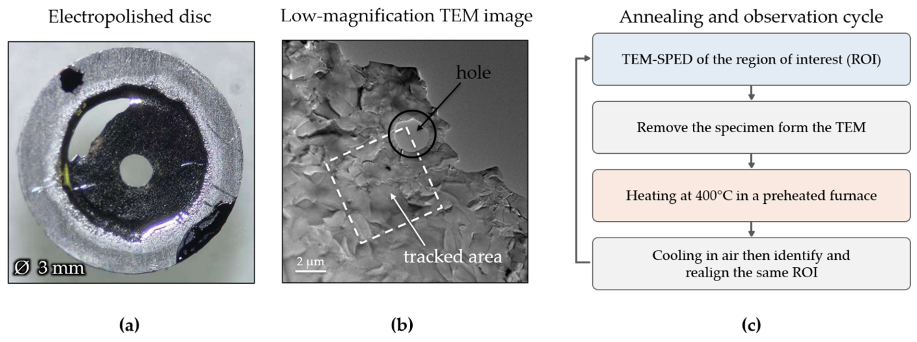
Figure 2.
Region of interest and phase-field initialization. (a) TEM-SPED orientation map at 0 min. The dashed box marks the 30 × 30 point (600 × 600 nm) region of interest, which lies 1.45 µm from the edge of the hole. The randomly colored circular area is the hole, where no pattern can be indexed. (b) The four grains of the region at 0 min, labeled φ1 - φ4 and assigned to the phase-field variables; colors denote the phase-field index and are used consistently in Figure 4 and Figure 6 and in Figure S1 and S2.
Figure 2.
Region of interest and phase-field initialization. (a) TEM-SPED orientation map at 0 min. The dashed box marks the 30 × 30 point (600 × 600 nm) region of interest, which lies 1.45 µm from the edge of the hole. The randomly colored circular area is the hole, where no pattern can be indexed. (b) The four grains of the region at 0 min, labeled φ1 - φ4 and assigned to the phase-field variables; colors denote the phase-field index and are used consistently in Figure 4 and Figure 6 and in Figure S1 and S2.
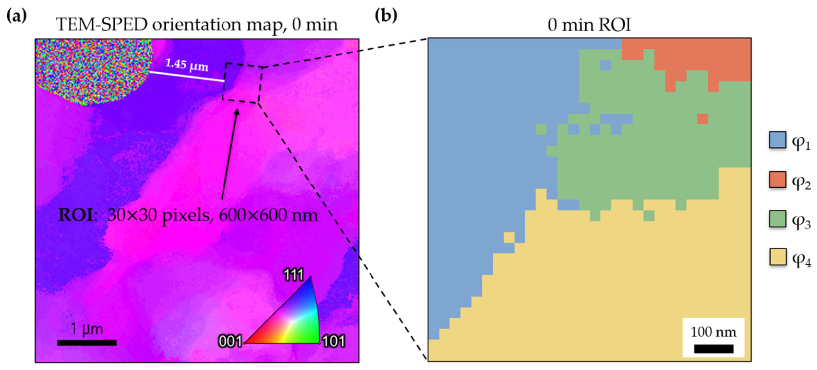
Figure 3.
Workflow of the multiphase-field–ensemble Kalman filter framework. The 0 min orientation map initializes the phase fields; 50 ensemble members are generated by perturbing the six mobilities about a mean of 0.132 with a standard deviation of 40% of the mean; each member is integrated for 200 steps, corresponding to 5 min; the augmented state, containing the phase fields and the six mobilities, is updated against the measured grain-label map; and the ensemble is restarted from the analyzed state. The cycle is repeated for the observations at 5, 10, 15 and 20 min. The ensemble-mean mobilities after the 20 min update define the inferred mobilities, which are used for DA-init; Direct is the same restart carried out with the initially assigned mobilities.
Figure 3.
Workflow of the multiphase-field–ensemble Kalman filter framework. The 0 min orientation map initializes the phase fields; 50 ensemble members are generated by perturbing the six mobilities about a mean of 0.132 with a standard deviation of 40% of the mean; each member is integrated for 200 steps, corresponding to 5 min; the augmented state, containing the phase fields and the six mobilities, is updated against the measured grain-label map; and the ensemble is restarted from the analyzed state. The cycle is repeated for the observations at 5, 10, 15 and 20 min. The ensemble-mean mobilities after the 20 min update define the inferred mobilities, which are used for DA-init; Direct is the same restart carried out with the initially assigned mobilities.
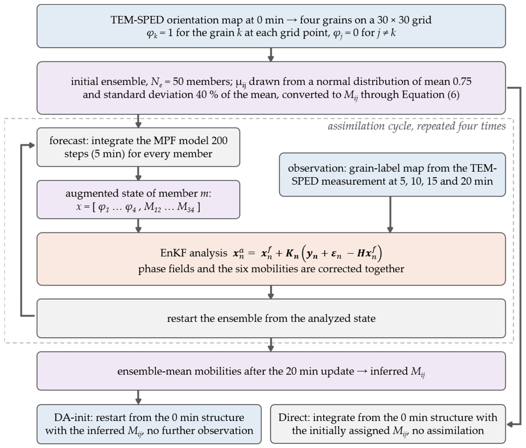
Figure 4.
Time-resolved observation of tracked area after cumulative annealing at 400 °C for 0, 5, 10, 15 and 20 min. (a) TEM images. (b) TEM-SPED orientation maps, colored by the crystal orientation parallel to the specimen normal according to the inverse pole figure key; the dashed box marks the 600 × 600 nm region of interest used for the simulations. (c) Grain-label maps of the region of interest, obtained from the orientation maps in (b) by the orientation grouping described in Section 2.3.
Figure 4.
Time-resolved observation of tracked area after cumulative annealing at 400 °C for 0, 5, 10, 15 and 20 min. (a) TEM images. (b) TEM-SPED orientation maps, colored by the crystal orientation parallel to the specimen normal according to the inverse pole figure key; the dashed box marks the 600 × 600 nm region of interest used for the simulations. (c) Grain-label maps of the region of interest, obtained from the orientation maps in (b) by the orientation grouping described in Section 2.3.
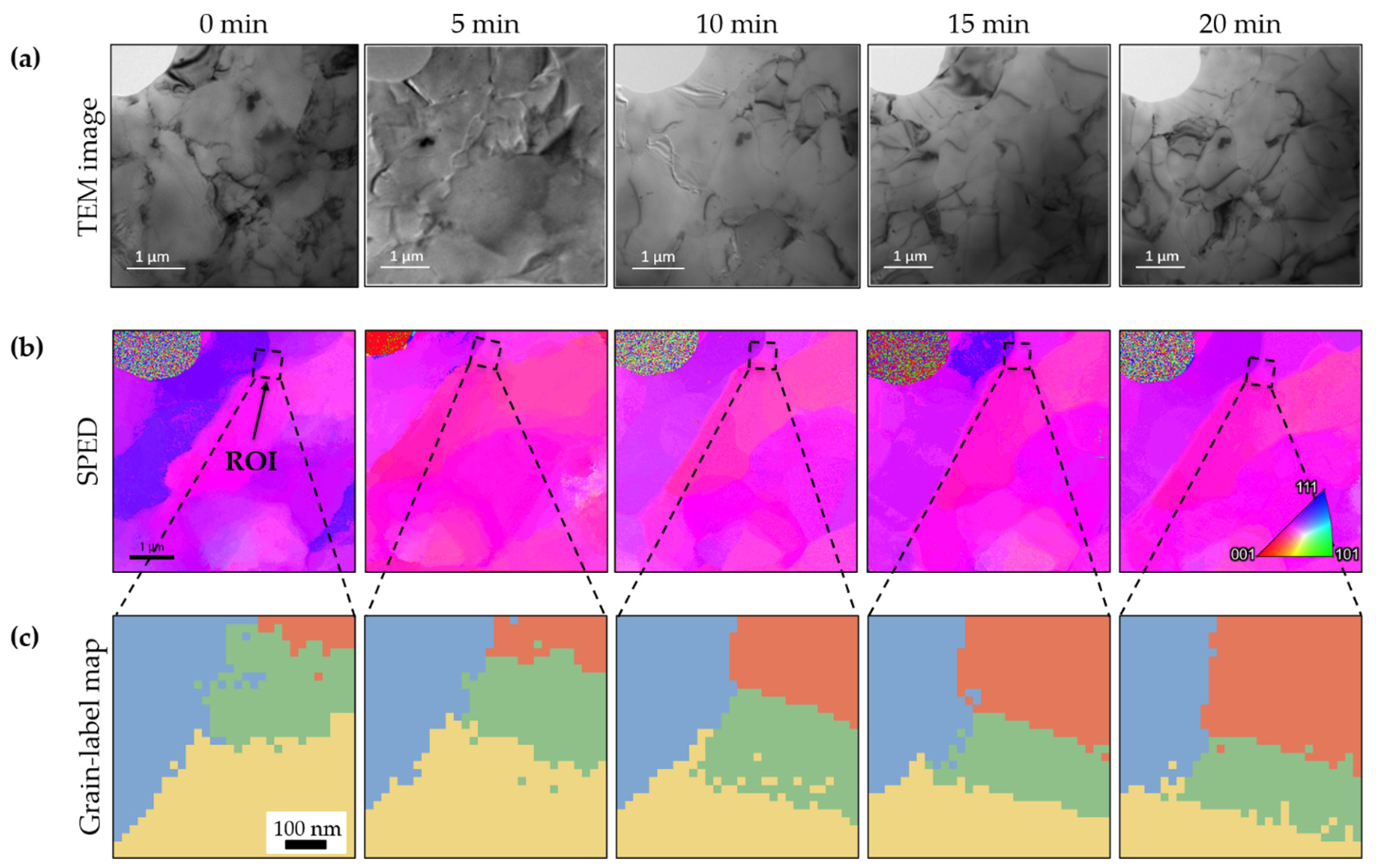
Figure 5.
Estimated grain-boundary mobilities over the four assimilation cycles. (a) Ensemble mean of the six mobilities; (b) ensemble standard deviation, on a logarithmic scale, computed over the 50 members with a population convention. Mobilities are the dimensionless coefficients of Equation (5) under the mapping of 5 min to 200 integration steps.
Figure 5.
Estimated grain-boundary mobilities over the four assimilation cycles. (a) Ensemble mean of the six mobilities; (b) ensemble standard deviation, on a logarithmic scale, computed over the 50 members with a population convention. Mobilities are the dimensionless coefficients of Equation (5) under the mapping of 5 min to 200 integration steps.
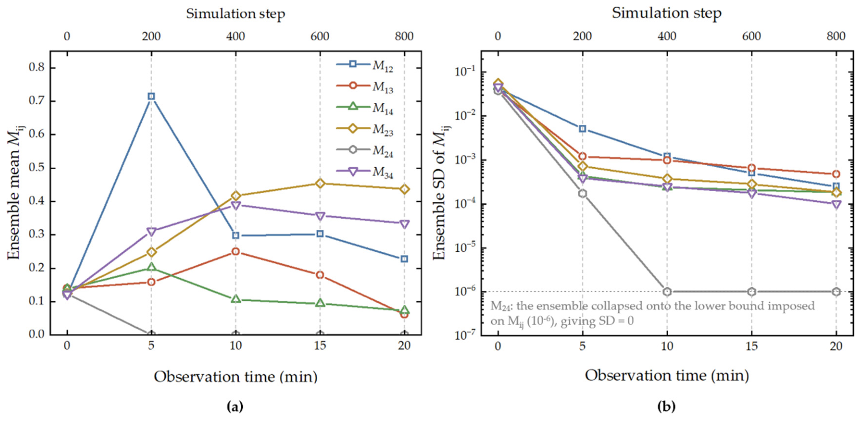
Figure 6.
Observed and simulated grain-label maps at 0, 5, 10, 15 and 20 min. (a) Observation; (b) DA-init; (c) Direct simulation, integrated throughout with the initial unassimilated mobilities. Colors denote the phase-field variables as in Figure 2. The growth of φ₂ and the shrinkage of φ₄ are reproduced in (b) but not in (c).
Figure 6.
Observed and simulated grain-label maps at 0, 5, 10, 15 and 20 min. (a) Observation; (b) DA-init; (c) Direct simulation, integrated throughout with the initial unassimilated mobilities. Colors denote the phase-field variables as in Figure 2. The growth of φ₂ and the shrinkage of φ₄ are reproduced in (b) but not in (c).
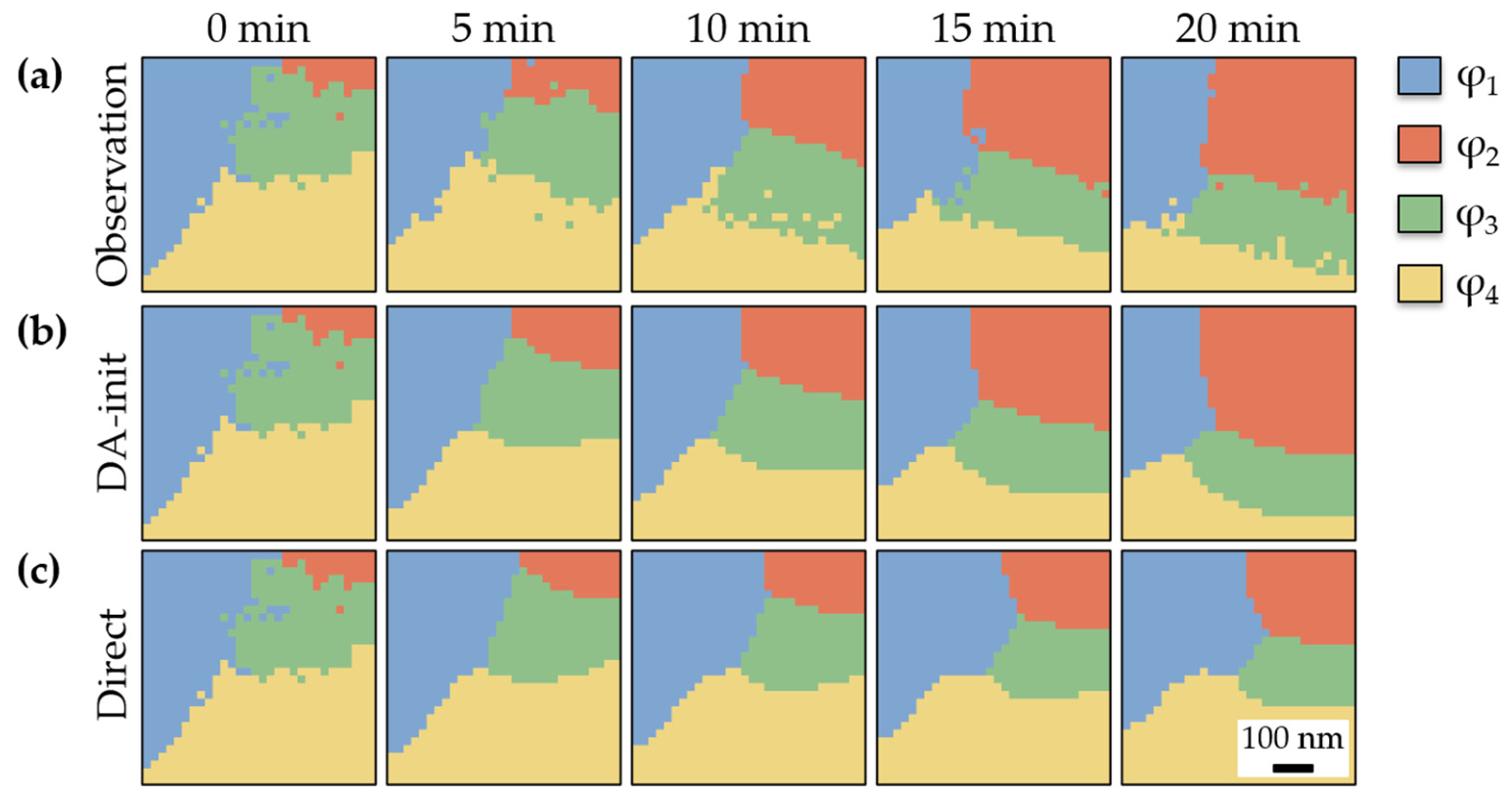
Figure 7.
Label agreement with the observation. Label agreement A(t) of the four cases with the observation at each observation time; the dotted line marks perfect agreement. At 5 min the DA forecast coincides with the Direct simulation, because it is integrated from the 0 min state and no update has yet occurred.
Figure 7.
Label agreement with the observation. Label agreement A(t) of the four cases with the observation at each observation time; the dotted line marks perfect agreement. At 5 min the DA forecast coincides with the Direct simulation, because it is integrated from the 0 min state and no update has yet occurred.
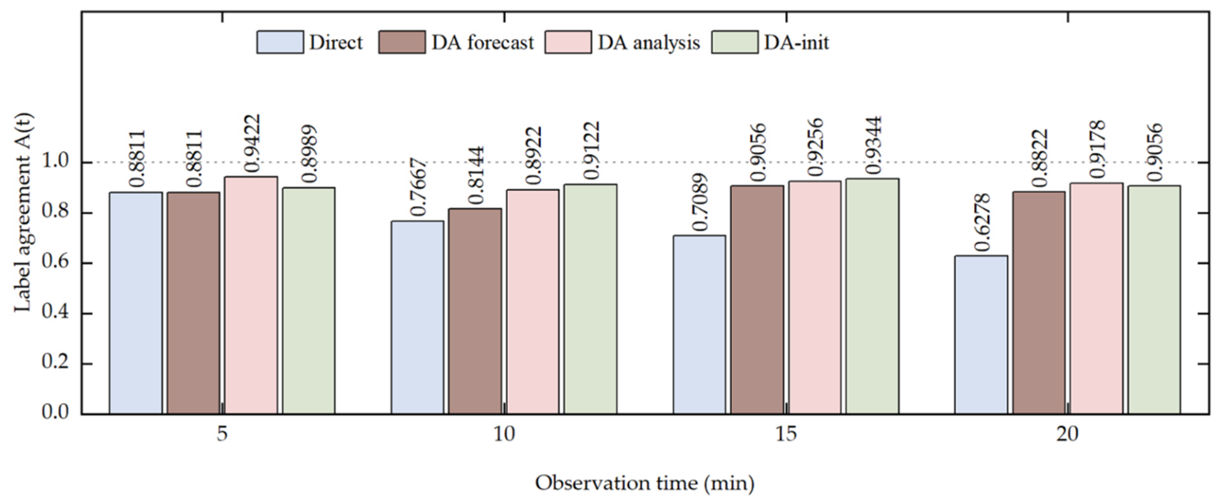
Figure 8.
Variation of the individual grain areas. (a–d) Grain areas Si(t) of φ₁ - φ₄ within the region of interest as a function of annealing time for the Direct (dashed), the simulation with data assimilation (thin line, showing the discontinuities produced by each update) and DA-init (thick line), with the observed areas as open circles. Note that one grid point corresponded to 4.0 × 10⁻⁴ µm².
Figure 8.
Variation of the individual grain areas. (a–d) Grain areas Si(t) of φ₁ - φ₄ within the region of interest as a function of annealing time for the Direct (dashed), the simulation with data assimilation (thin line, showing the discontinuities produced by each update) and DA-init (thick line), with the observed areas as open circles. Note that one grid point corresponded to 4.0 × 10⁻⁴ µm².
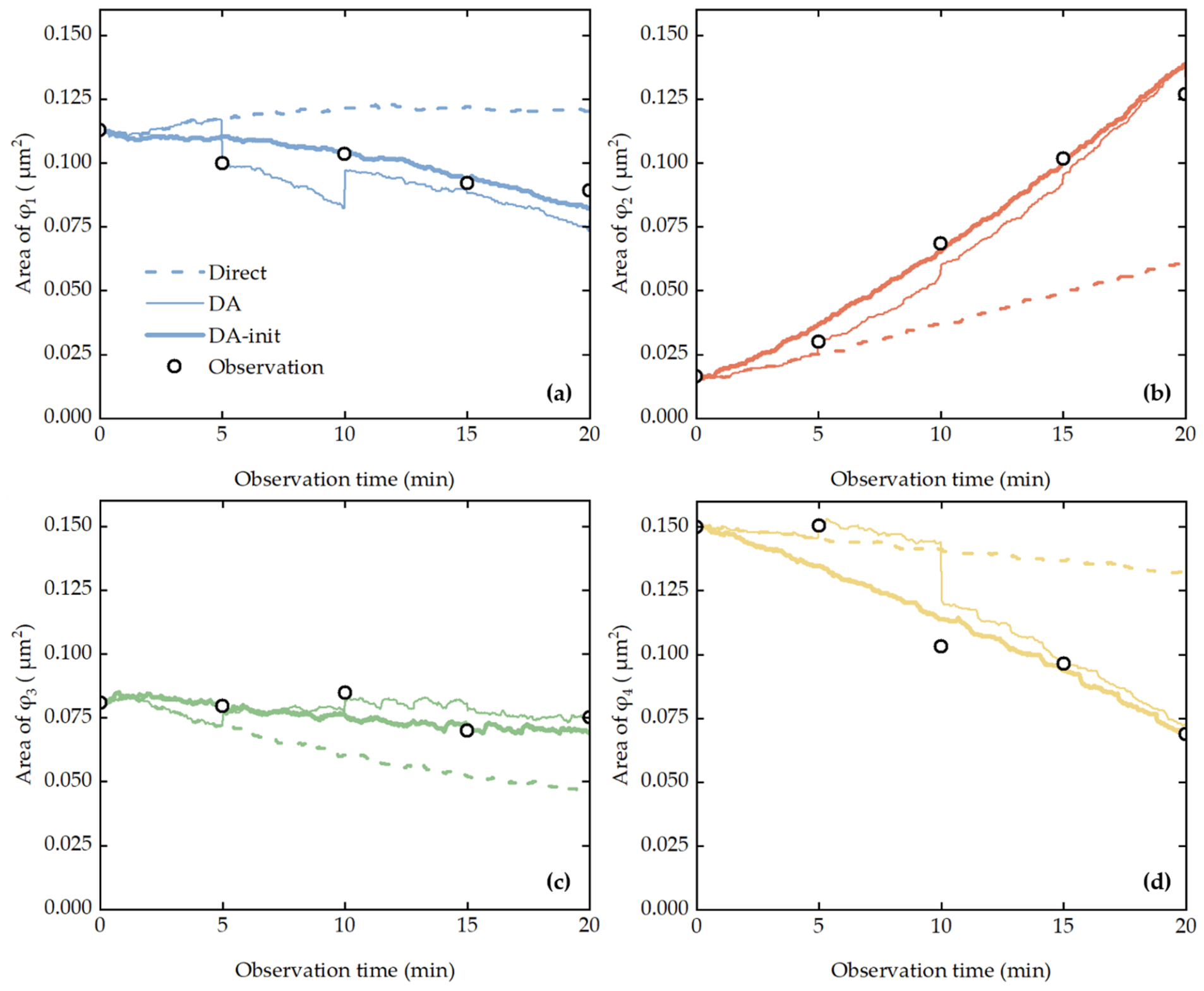
Figure 9.
Mobilities inferred using different numerical time-step sizes of 3.0, 1.5 and 1.0 s. The mobilities are normalized by the number of integration steps per 5 min interval.
Figure 9.
Mobilities inferred using different numerical time-step sizes of 3.0, 1.5 and 1.0 s. The mobilities are normalized by the number of integration steps per 5 min interval.
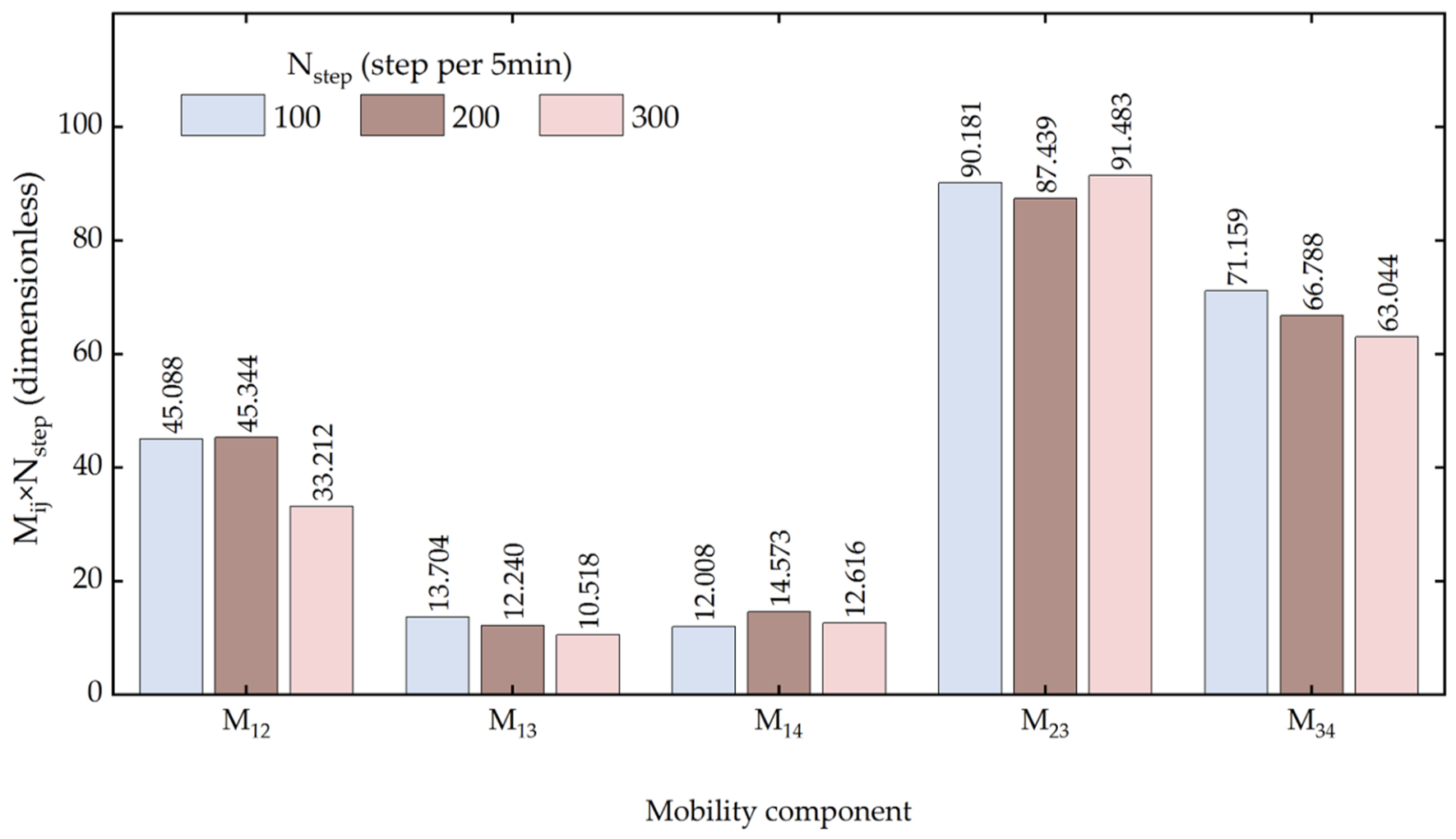

Table 1.
Summary of specimen preparation, annealing and TEM-SPED acquisition conditions.
| Item | Condition |
|---|---|
| Material | Pure aluminum(A1050) |
| Prior deformation | Cold rolling, 50% thickness reduction |
| Specimen geometry | Disc, 3 mm diameter, < 0.1 mm thick |
| Thinning | Twin-jet electropolishing (E.A. Fischione Instruments, Inc.) |
| Electrolyte | HNO3: CH3OH = 3: 7 |
| Electrolyte temperature | −30 °C |
| Voltage / Current | 25 V / 40 mA |
| Flow-rate setting | 7 |
| Annealing | Tubular electric furnace (Asahi Rika Manufacturing Co., Ltd.), pre-heated to 400 °C, 5 min per step |
| Cumulative annealing times | 0, 5, 10, 15, 20 min |
| Microscope | JEM-ARM200F (JEOL) |
| Holder | Double-tilt holder (JEOL) |
| Acceleration voltage | 200 kV |
| Acquisition mode | TEM-SPED (ASTAR, NanoMegas) |
| Acquisition area | 5.4 × 5.4 µm |
| Step size | 20 nm |
| Frame size | 270 × 270 points |
| Precession angle | 0.5° |
Table 2.
Multiphase-field and ensemble Kalman filter parameters.
| Group | Symbol | Quantity | Value |
|---|---|---|---|
| Grid | Nx×Ny | Grid points | 30 × 30 |
| Δx | Grid spacing | 20 nm | |
| Domain size | 600 × 600 nm | ||
| Boundary condition | Zero flux | ||
| Scaling | T | Annealing temperature | 673.15 K |
| Vm | Molar volume | 1.0 × 10⁻⁵ m3 mol-1 | |
| R | Gas constant | 8.3145 J mol-1 K-1 | |
| Microstructure | N | Grains (phase-field variables) | 4 |
| Independent mobilities | 6 (M12, M13, M14, M23, M24, M34) | ||
| Interfacial | δ | Interface width | 7Δx (140 nm) |
| γij | Grain-boundary energy | 0.5 J m−2 (4.47 × 10⁻² dimensionless) | |
| aij | Gradient-energy coefficient | 0.253 (dimensionless) | |
| Wij | Barrier height | 2.55 × 10⁻² (dimensionless) | |
| Eij | Driving force | 8.93 × 10⁻³(dimensionless) | |
| Time integration | Δt | Time step | 1 |
| Steps per observation interval | 200 (≡ 5 min) | ||
| EnKF | Ne | Ensemble size | 50 |
| μ0 | Prior mean interface mobility | 0.75 | |
| Prior standard deviation | 0.4μ0 | ||
| Resulting prior for Mij | mean 0.1322, SD 0.0529 | ||
| Assimilation cycles | 4 (at 5, 10, 15, 20 min) | ||
| H | Observation operator | Selects the phase-field block | |
| R | Observation-error covariance | σo2 I, σo = 1 × 10⁻² |
Table 3.
Agreement with the observation and inferred mobilities at 20 min.
| Case | Label agreement A(t) | Disagreeing points (of 900) | M12 | M13 | M14 | M23 | M24 | M34 |
|---|---|---|---|---|---|---|---|---|
| Direct | 0.6278 | 335 | 0.132 | 0.132 | 0.132 | 0.132 | 0.132 | 0.132 |
| DA forecast | 0.8822 | 106 | 0.3018 | 0.1802 | 0.0944 | 0.4547 | - | 0.3579 |
| DA analysis | 0.9178 | 74 | 0.2267 | 0.0612 | 0.0729 | 0.4372 | - | 0.3339 |
| DA-init | 0.9056 | 85 | 0.2267 | 0.0612 | 0.0729 | 0.4372 | - | 0.3339 |
Table 4.
Label agreement of DA-init with the observation at 20 min for the three assimilation intervals examined.
Table 4.
Label agreement of DA-init with the observation at 20 min for the three assimilation intervals examined.
| Steps per 5 min | Step duration (s) | Label agreement A(t) (DA-init) |
|---|---|---|
| 100 | 3.0 | 0.8833 |
| 200 | 1.5 | 0.9056 |
| 300 | 1.0 | 0.8900 |
Disclaimer/Publisher’s Note: The statements, opinions and data contained in all publications are solely those of the individual author(s) and contributor(s) and not of MDPI and/or the editor(s). MDPI and/or the editor(s) disclaim responsibility for any injury to people or property resulting from any ideas, methods, instructions or products referred to in the content. |
© 2026 by the authors. Licensee MDPI, Basel, Switzerland. This article is an open access article distributed under the terms and conditions of the Creative Commons Attribution (CC BY) license (http://creativecommons.org/licenses/by/4.0/).
Copyright: This open access article is published under a Creative Commons CC BY 4.0 license, which permit the free download, distribution, and reuse, provided that the author and preprint are cited in any reuse.