

Submitted:
09 September 2026
Posted:
10 September 2026
You are already at the latest version
Abstract
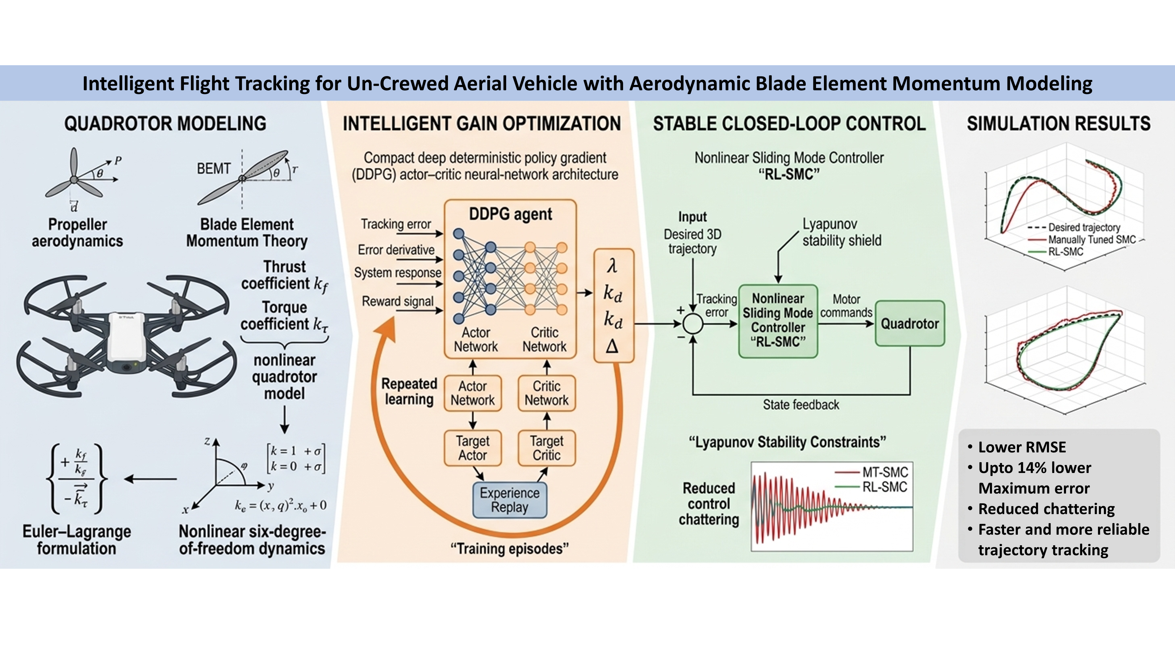
Quadrotors attract broad military and civilian interest, yet their underactuated, highly coupled, and nonlinear dynamics make precise control difficult. While Sliding Mode Control (SMC) offers robust trajectory tracking, tuning its parameters—such as sliding surfaces and switching gains—remains a tedious manual task. To overcome this, we present an adaptive SMC framework integrated with an Actor-Critic Deep Reinforcement Learning (DRL) algorithm for automated gain synthesis. A full 6-DoF quadrotor model is derived via Euler-Lagrange mechanics, with aerodynamic coefficients estimated using Blade Element Momentum theory. The DRL agent dynamically adjusts SMC gains online, reducing chattering while ensuring accurate altitude and trajectory tracking. Lyapunov's direct method rigorously establishes asymptotic stability of the closed-loop system. Comparative simulations show that the proposed DRL-SMC approach consistently outperforms conventional fixed-gain baselines, achieving lower Root Mean Squared Error across complex flight profiles.
Keywords:
quadcopter modeling
; lyapunov stability
; sliding mode control
; nonlinear control
; artificial intelligence
; reinforcement learning
; unmanned aerial vehicle
1. Introduction
Unmanned aerial vehicles (UAVs), particularly quadrotors, have become an important research topic because they combine vertical take-off and landing, high maneuverability, and relatively low operating cost[1,2,3,4,5]. They had been widely used in variety of real-world applications which include environmental exploration, search and rescue missions and aerial mappings [2,6,7,8]. The development of a flight controller generally begins with the formulation of a linear or nonlinear mathematical model of the UAV [9]. This model provides the basis for analyzing the vehicle dynamics and designing a closed-loop feedback controller. A wide range of control methods has therefore been investigated, including proportional-integral-derivative (PID) control, sliding-mode control (SMC), control, backstepping, linear-quadratic regulation (LQR), and adaptive or learning-based methods [10,11,12,13,14,15,16,17].
These techniques have been applied to attitude stabilization, position regulation, trajectory tracking, and obstacle-avoidance tasks [11,12,13,14,17,18]. Conventional PID controllers remain attractive because of their simple structure and low computational cost, whereas nonlinear and robust methods are often preferred when stronger guarantees are required in the presence of disturbances and parameter variations.
Accurate modeling of the aerodynamic forces and moments is also important for assessing controller performance. Blade-element momentum theory (BEMT) is one of the most commonly used approaches for estimating rotor and propeller aerodynamic loads [19,20]. Earlier quadrotor studies combined aerodynamic modeling with flight-dynamics analysis and experimental control validation[21,22] . More detailed formulations have also incorporated variations in rotor aerodynamics and motor operating conditions to improve thrust prediction and control performance [23]. These studies demonstrate that aerodynamic effects can become significant during aggressive maneuvers and should not be neglected when a high-fidelity model is required.
Because quadrotor dynamics are nonlinear and strongly coupled, stability analysis is an essential part of controller design. Lyapunov-based methods are frequently used to establish stability properties and to evaluate the behavior of nonlinear controllers. Several studies have developed Lyapunov-based sliding-mode and robust adaptive controllers for quadrotor trajectory tracking and attitude regulation[24,25,26,27]. Other work has investigated the relationship between Lyapunov stability conditions and PID or adaptive backstepping control laws [28,29,30,31]. Comparative studies have further examined the performance of PD, PID, and sliding-mode controllers for multirotor systems under different operating conditions [32]. Related research on vehicles carrying liquid payloads has shown that fluid motion can introduce additional disturbances and coupling effects that must be considered in the control design [9,33].
In parallel with these model-based approaches, reinforcement learning (RL) and adaptive dynamic programming have attracted increasing attention for nonlinear flight-control problems [34]. RL-based attitude controllers have been developed for fixed-wing UAVs and quadrotors, with reported improvements in adaptation and tracking performance under uncertain or changing conditions [35]. Deep-RL methods have also been applied to autonomous UAV tracking and landing, demonstrating their potential for handling complex maneuvering tasks [36]. Nevertheless, learning-based controllers may require substantial training data and careful safety constraints before deployment on physical platforms. Combining a physically derived nonlinear model with a stability-oriented controller and an RL-based parameter adaptation mechanism can therefore provide a useful compromise between interpretability, robustness, and adaptability.
In this work, the nonlinear dynamics of an X-configuration quadrotor are formulated using the Euler–Lagrange method. The rotor thrust and torque coefficients are estimated using BEMT. The main contribution is a Lyapunov-based altitude and yaw control strategy in which reinforcement learning is used to obtain locally optimized parameters for the sliding-mode controller. The resulting controller is designed to stabilize the six-degree-of-freedom quadrotor system while reducing altitude and yaw tracking errors, as illustrated in Figure 1.
2. Mathematical Modeling
This section contains an overview of the quadrotor kinematics and dynamics. The general drone control mechanism included in the suggested methodology is shown in Figure 1. RL optimized SMC controllers, together with blade aerodynamics, actuator kinematics, and nonlinear quadrotor dynamics, are employed for optimal feedback control of quadrotor altitude and position. Description of geometric parameters and coordinate reference frames is included here which is necessary for understanding the quadrotor dynamics. Specifications of DJI Tello Drone[37] are used for this study. The mass m is 80 gm whereas, diagonal length is 0.119 m.
Figure 2 covers two different reference frames required to represent quadrotor system. denotes Earth-fixed or Inertial coordinate system which is considered as primary frame of reference and denotes body frame which defines the location of points relative to the quadrotor body.
In order to make the equations simple, following assumptions are considered true:
- We assumed quadrotor as symmetric rigid body with constant mass distribution.
- The center of gravity (CG) of the drone and its geometric center coincide.
- Thrust vector is assumed to be perpendicular to the drone frame.
- Gravity direction is positive opposite to the thrust vector.
- Direction of motion in clockwise (CW) is considered positive, while counter clockwise (CCW) is considered negative.
- Propellers with odd indices indicate CW rotation, while propellers with even indices indicate CCW rotation as seen in Figure 2.
The location of a quadrotor in inertial frame of reference is given by vector whereas, represents orientation of vector Euler angles. Roll, Pitch and Yaw angles are denoted by , and , respectively. State vector for such system is written as:
2.1. Kinematics
The linear velocity v and angular velocity ω can be defined in inertial frame as:
where , , denotes the linear velocity vector of body frame and denotes a vector of the quadrotor body rates. is orthogonal rotational and is angular transformation matrix from body frame to inertial frame defined[38].
2.2. Dynamics
In essence, Lagrangian mechanics is an optimization process that depends on the difference between the system’s kinetic and potential energy. The Lagrangian is defined as the difference between kinetic and potential energies:
where term, is the Jacobian Matrix, is termed as inertia tensor, and denotes gravitational constant.
The moment of inertias of DJI Tello Drone are estimated experimentally using the bifilar pendulum method [39], since this method has been found more robust to external disturbances when compared to conventional pendulum methods.
In the above equation subscript represents an element of the inertia tensor, and denotes the perpendicular distance between both strings and the axis of rotation, whereas, is the average length of the strings, and is average time period for oscillations in experiments. The Euler-Lagrange expression can be written as:
where is the net thrust and is the torque acting on the body of the quadrotor. Eq. 6 can be simplified and solved into the generalized form of robot dynamics:
where denotes the inertial matrix which is dependent on the geometric properties of the quadrotor. is known called the Coriolis matrix, which is composed of gyroscope and centripetal terms, and is gravitational vector, derived from potential energy equation. These terms can be expressed in array form as:
where is a 3 3 diagonal mass matrix, and .
The right-hand side of Eq. 6 represents the control effectiveness matrix for the configuration model, and can also expressed in its matrix form:
is defined as the angle between and the arm in CW direction, is the distance from CG of quadrotor to center of the motor, rotational speed of nth motor is denoted by while = , . Total thrust generated is , aerodynamic thrust coefficient is , aerodynamic torque coefficient is denoted by , while is denoted by and is denoted by . Eq. 7 is rearranged and separated into linear and rotational acceleration components:
2.3. Propeller Aerodynamics
Understanding the different aerodynamic impacts of the propellers and their interaction with the quadrotor’s rigid body motion is essential. Thrust and torque coefficients are considered critical parameters for BEMT in order to evaluate the performance of quadrotor propeller based on its mechanical and geometric parameters. [40]considered uniform inflow model for hover and edgewise flight. We assume the following to further simplify the equations:
- Thin air foil theory suggests, lift curve passes through the origin and lift slope is
- Axial velocity component is imperceptible when compared to tangential velocity.
- Viscosity effects are ignored.
- In-plane velocities are negligible.
- Inflow angle is small.
According to thin airfoil theory, the effective angle of attack and sectional lift coefficient is defined as[41]:
where is the sectional pitch angle, is the sectional zerolift angle of attack, and the inflow angle , where is the radial distance of the center of the hub to the blade element. Inflow coefficient can be calculated by solving the following equations iteratively [38]:
where is called the advance ratio, is known as the solidity ratio, is the rotor thrust coefficient, and is the rotor power coefficient. Blade tip vortices are considered as dominant feature of rotor wakes. Empirical models are often used to cater for non-uniform inflow effects. [42]suggested that the subsequent inflow at the rotor disc may be characterized by a longitudinally varying, non-uniform first-harmonic model of the form:
and are the factors that contribute to flow changes along the length and width of the wake. is the induced flow ratio from the uniform momentum theory, and is the blade azimuth angle[43]. Experimental models for and are derived from[44]. Thrust and torque coefficients can be estimated by using converged values of and can be estimated as:
where denotes the air density and is the radius of blade. Using linearization around the hover point in equation (9) leads to following equations for altitude and yaw of quadrotor.
3. Stability And Control
This section introduces sliding mode technique-based control law for stabilizing the altitude and yaw of a quad-rotor aircraft to a desired reference during a flight mission. The control involves coordination of all four rotors to achieve the desired altitude and yaw control.
3.1. Sliding Mode Control
SMC technique is an approach of variable structure control (VSC). The objective of SMC deals with constraining the error vector to reach a desired state through two parts[45]. The first step is creating a control law that, during the reaching phase, directs the error vector in the direction of a sliding surface. This part is characterized by the control being switched on different sides of the sliding surface. The error vector is confined to the sliding surface and the system tracks the dynamics imposed by the sliding surface equations in the second part which is referred as equivalent control[46]. To stabilize the quadrotor, four control equations are used to maintain the system’s altitude and orientation close to the desired reference value, despite external disturbances. The signals are utilized to regulate the altitude, roll, pitch, and yaw of the quadrotor, respectively.
Equation (18) represents the sliding surface, where is the system error, is the derivative of the error, and is a positive constant. The value of can be selected based on the desired performance criteria. The control input signals are designed such that the error vector approaches and remains on the sliding surface, ensuring the desired system behavior. The control law, is a mathematical expression defined as:
where represents the continuous part of the control law and represents the discontinuous part. The continuous part represents a smooth, continuous control input to the system while the discontinuous part represents a sudden change in the control input that leads to a discontinuity in the system’s behavior.
Equation (20) can be rewritten as,
where, is tuning parameter responsible for reaching phase and is nonlinear function of . We can reduce the chattering problem if we rewrite equation (21) as,
is a tuning parameter used to reduce the chattering effect. The equivalent control procedure is utilized to determine . The sliding surface for quadrotor error can be written by using (18) as,
Using sliding condition
Replacing the values and we get equation (26) below,
Substituting values from equation (18), sliding condition is expressed as,
Using equation (20) and (21), setting , we get expression,
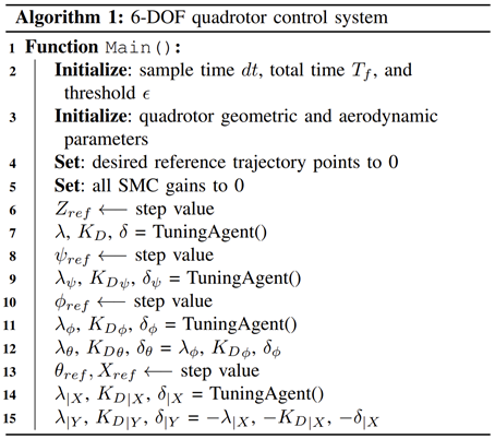
Algorithm 1 shows the steps involved in 6-DOF quadrotor control system.
3.2. Stability Analysis
For a given control system, the Lyapunov function is a scalar function that satisfies two conditions: positive-definiteness and monotonicity. Positive-definiteness means that the function is positive for all non-zero values of the state, while monotonicity means that the function decreases over time along the solutions of the system. The control of the altitude reference and attitude of a quadrotor is achieved through the use of the Lyapunov stability-based method, which directly focuses on attitude control of the quadrotor. The equilibrium point is defined as , and represents a compact region near in . The continuous Lyapunov function is used to meet the requirements.
Consider where and are the desired attitude angles for the quadrotor. As the angular velocities will be zero at the stabilization point, their time derivatives will also be zero. The function for yaw is described as a positive definite Lyapunov function at the desired position.
The equation for derivative is written as,
The equation of motion at equilibrium point for yaw can be written as,
Control Input equation leads to,
Equation of motion for yaw can be rewritten as,
The Lyapunov theorem provides simple stability for the equilibrium. Asymptotic stability is achieved through the application of LaSalle’s theorem, as the maximum invariance rotation subsystem that is controlled within the set is confined only to the equilibrium point. The Lyapunov stability function and its derivative with respect to the angles and altitude are described as,
Taking the derivative of above equation, we get
Control input is given to system for stability,
Replacing (40) in (39) leads to,
The constant described by equation (41) is a positive constant that is only negative semi-definite.
3.3. Optimal Gain Tuning using Reinforcement Learning
Deep deterministic policy gradient (DDPG) algorithm is chosen as the RL component of the controller due to its ability to obtain a deterministic policy and its sample efficiency compared to other actor-critic methods as shown in Figure 3. In the machine learning branch of reinforcement learning, an agent learns to interact with its surroundings in a way that maximizes a cumulative reward signal over time[47]. Learning a policy that maximizes the predicted cumulative reward is the goal. The agent’s behavior is described by a policy that associates states with actions. Value functions, which calculate the predicted cumulative reward of performing a certain action in a given state, are used by RL algorithms[48]. The Q-learning technique is a popular method that iteratively updates estimates of the anticipated reward for every state-action pair in order to learn the best action-value function[49]. Using deep neural networks as function approximators, deep reinforcement learning (DRL) is a well-liked method for RL that estimates value functions and policies in high dimensional, continuous state and action spaces[50].
Natural language processing, gaming, robotics, and many more fields have seen the effective use of DRL[51]. Without requiring human feature engineering, DRL can learn directly from high dimensional sensory inputs like 1-D audio signals or 2-D visuals, which is one of its main benefits.
This makes it ideal for applications where the input space can be rather complicated and extensive, such visual object recognition [52]. The target networks slowly monitor the learned networks in order to improve their convergence stability during the learning process by maximizing the agent’s cumulative reward:
where is called the discount factor, and for the scope of this study, is intuitively defined as:
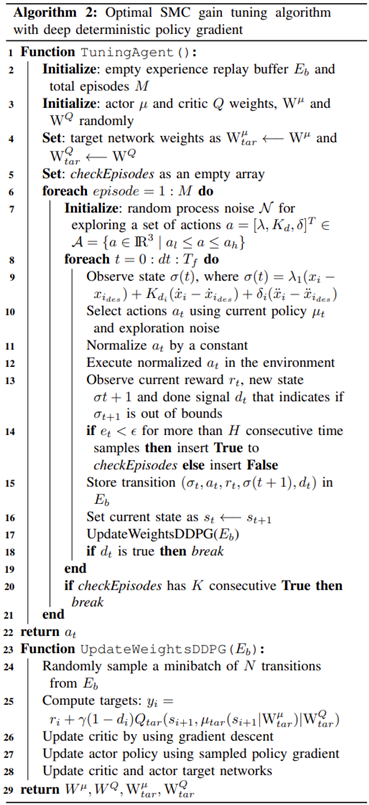
rewards the agent when the squared error term is 0.5 or less. penalizes the agent if it exceeds 25% of the desired step value or goes in the negative direction during training (given positive step input). penalizes the agent exponentially with respect to error. and punishes the agent with increasing control effort and simulation time, respectively. Using this reward function, the optimal gain auto-tuning process for a 6-DOF quadrotor is outlined in Algorithm 2.
4. Simulation and Results
The MATLAB/Simulink platform serves as the foundation for the control strategy experiment in this section. Two different trajectories were employed to demonstrate the efficacy of results. This study’s goal is to assess the validity and efficacy of the proposed control strategy. The comparative experiments were conducted between two control techniques: manually tuned (MT)-SMC and RL-SMC (auto-tuned) for a dynamic model of a quadrotor. Auto-tuned controller refers to those optimal sliding mode gains which are obtained using RL.
Figure 4 shows the individual trajectory tracking comparison in X, Y, and Z directions between MT-SMC and RL-SMC of quadrotor. Here, quadrotor followed the trajectory 1 which involved rather simple maneuvers with step commands.
Error comparison for all directions between actual and desired trajectories (trajectory 1 case) can be seen in Figure 5. It can be noted that RL tuned SMC minimizes the error terms, since, the manually tuned SMC carries the inherent property of chattering.
Figure 6 shows the individual trajectory tracking comparison in X, Y, and Z directions for MT-SMC and RL-SMC of quadrotor. In this case, a relatively complex and longer trajectory (trajectory 2) has been tested with the both manual and auto-tuned controllers.
Error comparison between actual and desired trajectories for all directions can be seen in Figure 7. It can be inferred from the results that the tracking error for manually tuned SMC is relatively higher that RL tuned SMC with optimal gains.
Moreover, during this activity, it is observed that as nonlinearity increases, the number of episodes needed to attain convergence increases, with Z-Agent achieving convergence in 35 episodes, ψ-Agent in 79 episodes, ϕ-Agent in 145 episodes, and X-Agent in 338 episodes. A tabular comparison of the gains obtained from the two methods, for all directions in both test trajectories, is shown in Table 1.
Similarly, Table 2 describes the performance comparison of both the controllers in terms of RMSE and maximum error for all the employed test cases.
5. Discussion
This work implements a systematic auto-tuning framework for a 6-degree-of-freedom nonlinear quadrotor using a sliding mode controller, though the approach extends to other mechanical systems. Blade aerodynamics are modeled via blade element momentum theory, while the vehicle's dynamic equations are derived using the Euler-Lagrange formalism. A closed-loop cascaded architecture governs trajectory tracking, with SMC serving as the regulation law. Lyapunov's direct method confirms closed-loop stability, with adaptations incorporated to align the SMC design for robotic manipulators. In contrast to fixed-gain baselines, we embed a deep reinforcement learning agent specifically, DDPG, within the control loop to automatically search for and update the optimal controller gains online. This agent continuously adapts the gains using real-time state feedback, which enhances robustness under highly nonlinear and uncertain operating conditions. For experimental validation, we choose the DJI Tello drone as our physical platform, determining its mass, dimensions, and moments of inertia through bifilar suspension tests, while the thrust and torque coefficients are obtained numerically from BEMT computations. The identified parameters show close agreement with reported literature values, confirming consistency of our identification procedure. The DRL-optimized gains satisfy all prescribed stability bounds.
Author Contributions
“Conceptualization, Kamal Mazhar Malik and Arshad Syed Muhammad Nashit; methodology, Arshad Syed Muhammad Nashit; software, Li Qiang; validation, Arshad Syed Muhammad Nashit; formal analysis, Arshad Syed Muhammad Nashit; investigation, Kamal Mazhar Malik.; resources, Li Qiang ; data curation, Kamal Mazhar Malik; writing—original draft preparation, Kamal Mazhar Malik.; writing—review and editing, Mingqi Chen; visualization, Kamal Mazhar Malik; supervision, Li Qiang and Ming Zhong; project administration, Li Qiang and Zhong Ming; funding acquisition, Li Qiang.
Funding
This work was supported by the Natural Science Foundation of Top Talent of SZTU (Grant No. GDRC202411).
Conflicts of Interest
Declare conflicts of interest or state “The authors declare no conflicts of interest.” Authors must identify and declare any personal circumstances or interest that may be perceived as inappropriately influencing the representation or interpretation of reported research results. Any role of the funders in the design of the study; in the collection, analyses or interpretation of data; in the writing of the manuscript; or in the decision to publish the results must be declared in this section. If there is no role, please state “The funders had no role in the design of the study; in the collection, analyses, or interpretation of data; in the writing of the manuscript; or in the decision to publish the results”.
References
- Idrissi, M.; Salami, M.; Annaz, F. A Review of Quadrotor Unmanned Aerial Vehicles: Applications, Architectural Design and Control Algorithms. J. Intell. Robot. Syst. Theory Appl. 2022, 104, 22. [Google Scholar] [CrossRef]
- Shakhatreh, H.; Sawalmeh, A.; Hayajneh, K.F.; Abdel-Razeq, S.; Malkawi, W.; Al-Fuqaha, A. A Systematic Review of Interference Mitigation Techniques in Current and Future UAV-Assisted Wireless Networks. IEEE Open J. Commun. Soc. 2024, 5, 2815–2846. [Google Scholar] [CrossRef]
- Doornbos, J.; Bennin, K.E.; Babur, O.; Valente, J. Drone Technologies: A Tertiary Systematic Literature Review on a Decade of Improvements. IEEE Access 2024, 12, 23220–23239. [Google Scholar] [CrossRef]
- Guebsi, R.; Mami, S.; Chokmani, K. Drones in Precision Agriculture: A Comprehensive Review of Applications, Technologies, and Challenges. Drones 2024, 8. [Google Scholar] [CrossRef]
- Zurita-Gil, M.A.; Ortiz-Torres, G.; Sorcia-Vázquez, F.D.J.; Rumbo-Morales, J.Y.; Gascon Avalos, J.J.; Reynoso-Romo, J.R.; Rosas-Caro, J.C.; Brizuela-Mendoza, J.A. Nonlinear Control Design for a PVTOL UAV Carrying a Liquid Payload with Active Sloshing Suppression. Technologies 2026, 14. [Google Scholar] [CrossRef]
- Reddy Maddikunta, P.K.; Hakak, S.; Alazab, M.; Bhattacharya, S.; Gadekallu, T.R.; Khan, W.Z.; Pham, Q.V. Unmanned Aerial Vehicles in Smart Agriculture: Applications, Requirements, and Challenges. IEEE Sens. J. 2021, 21, 17608–17619. [Google Scholar] [CrossRef]
- Calamoneri, T.; Coro, F.; Mancini, S. A Realistic Model to Support Rescue Operations after an Earthquake via UAVs. IEEE Access 2022, 10, 6109–6125. [Google Scholar] [CrossRef]
- Wang, Z.; Dong, W. A Collaborative Stereo Camera with Two UAVs for Long-Distance Mapping of Urban Buildings. IEEE Int. Conf. Intell. Robot. Syst. 2024, 7944–7951. [Google Scholar] [CrossRef]
- Zurita-Gil, M.A.; Ortiz-Torres, G.; Sorcia-Vázquez, F.D.J.; Rumbo-Morales, J.Y.; Gascon Avalos, J.J.; Reynoso-Romo, J.R.; Rosas-Caro, J.C.; Brizuela-Mendoza, J.A. Nonlinear Control Design for a PVTOL UAV Carrying a Liquid Payload with Active Sloshing Suppression. Technologies 2026, 14, 31. [Google Scholar] [CrossRef]
- Khalid, A.; Mushtaq, Z.; Arif, S.; Kamran, Z.E.B.; Khan, M.A.; Bakshi, S. Control Schemes for Quadrotor UAV: Taxonomy and Survey. ACM Comput. Surv. 2024, 56. [Google Scholar] [CrossRef]
- Almakhles, D.J. Robust Backstepping Sliding Mode Control for a Quadrotor Trajectory Tracking Application. IEEE Access 2020, 8, 5515–5525. [Google Scholar] [CrossRef]
- Kerma, M.; Mokhtari, A.; Abdelaziz, B.; Orlov, Y. Nonlinear H ∞ Control of a Quadrotor (UAV), Using High Order Sliding Mode Disturbance Estimator. Int. J. Control 2012, 85, 1876–1885. [Google Scholar] [CrossRef]
- Kang, B.; Miao, Y.; Liu, F.; Duan, J.; Wang, K.; Jiang, S. A Second-Order Sliding Mode Controller of Quad-Rotor UAV Based on PID Sliding Mode Surface with Unbalanced Load. J. Syst. Sci. Complex. 2021, 34, 520–536. [Google Scholar] [CrossRef]
- Okyere, E.; Bousbaine, A.; Poyi, G.T.; Joseph, A.K.; Andrade, J.M. LQR Controller Design for Quad-rotor Helicopters. J. Eng. 2019, 2019, 4003–4007. [Google Scholar] [CrossRef]
- Sun, X.; Quan, Z.; Zhang, F.; Li, Y.; Wang, C.; Si, W.; Ni, W.; Guan, R.; Wu, Y.; Shen, M.; et al. Dynamic Compact Consensus Tracking for Aerial Robots. Proc. IEEE Int. Conf. Robot. Autom. 2025, 6793–6800. [Google Scholar] [CrossRef]
- Elagib, R.; Karaasrlan, A. Implementation and Stabilization of a Quadcopter Using Arduino and the Combination of LQR and SMC Methods. J. Eng. Res. Rep. 2022, 23, 42–58. [Google Scholar] [CrossRef]
- Noordin, A.; Mohd Basri, M.A.; Mohamed, Z.; Mat Lazim, I. Adaptive PID Controller Using Sliding Mode Control Approaches for Quadrotor UAV Attitude and Position Stabilization. Arab. J. Sci. Eng. 2021, 46, 963–981. [Google Scholar] [CrossRef]
- Xu, Z.; Chen, B.; Zhan, X.; Xiu, Y.; Suzuki, C.; Shimada, K. A Vision-Based Autonomous UAV Inspection Framework for Unknown Tunnel Construction Sites With Dynamic Obstacles. IEEE Robot. Autom. Lett. 2023, 8, 4983–4990. [Google Scholar] [CrossRef]
- Kovačević, A.; Svorcan, J.; Hasan, M.S.; Ivanov, T.; Jovanović, M. Optimal Propeller Blade Design, Computation, Manufacturing and Experimental Testing. Aircr. Eng. Aerosp. Technol. 2021, 93, 1323–1332. [Google Scholar] [CrossRef]
- Tai, M.; Lee, W.; Kim, D.; Park, D. Improvements in Robustness and Versatility of Blade Element Momentum Theory for UAM/AAM Applications. Aerospace 2025, 12. [Google Scholar] [CrossRef]
- Hoffmann, G.M.; Huang, H.; Waslander, S.L.; Tomlin, C.J. Quadrotor Helicopter Flight Dynamics and Control: Theory and Experiment. Collect. Tech. Pap.-AIAA Guid. Navig. Control Conf. 2007, 2, 1670–1689. [Google Scholar] [CrossRef]
- Huang, H.; Hoffmann, G.M.; Waslander, S.L.; Tomlin, C.J. Aerodynamics and Control of Autonomous Quadrotor Helicopters in Aggressive Maneuvering. Proc. IEEE Int. Conf. Robot. Autom. 2009, 3277–3282. [Google Scholar] [CrossRef]
- Bangura, M.; Mahony, R. Thrust Control for Multirotor Aerial Vehicles. IEEE Trans. Robot. 2017, 33, 390–405. [Google Scholar] [CrossRef]
- Le Nhu Ngoc Thanh, H.; Hong, S.K. Quadcopter Robust Adaptive Second Order Sliding Mode Control Based on PID Sliding Surface. IEEE Access 2018, 6, 66850–66860. [Google Scholar] [CrossRef]
- Shao, X.; Liu, J.; Cao, H.; Shen, C.; Wang, H. Robust Dynamic Surface Trajectory Tracking Control for a Quadrotor UAV via Extended State Observer. Int. J. Robust. Nonlinear Control 2018, 28, 2700–2719. [Google Scholar] [CrossRef]
- Xu, L.X.; Ma, H.J.; Guo, D.; Xie, A.H.; Song, D.L. Backstepping Sliding-Mode and Cascade Active Disturbance Rejection Control for a Quadrotor UAV. IEEE/ASME Trans. Mechatron. 2020, 25, 2743–2753. [Google Scholar] [CrossRef]
- Ahn, H.; Hu, M.; Chung, Y.; You, K. Sliding-Mode Control for Flight Stability of Quadrotor Drone Using Adaptive Super-Twisting Reaching Law. Drones 2023, 7. [Google Scholar] [CrossRef]
- Dong, J.; He, B. Novel Fuzzy PID-Type Iterative Learning Control for Quadrotor UAV. Sensors 2019, 19, 24. [Google Scholar] [CrossRef]
- Noordin, A.; Basri, M.A.M.; Mohamed, Z. Simulation and Experimental Study on Pid Control of a Quadrotor MAV with Perturbation. Bull. Electr. Eng. Inform. 2020, 9, 1811–1818. [Google Scholar] [CrossRef]
- Xu, L.X.; Ma, H.J.; Guo, D.; Xie, A.H.; Song, D.L. Backstepping Sliding-Mode and Cascade Active Disturbance Rejection Control for a Quadrotor UAV. IEEE/ASME Trans. Mechatron. 2020, 25, 2743–2753. [Google Scholar] [CrossRef]
- Bu, Y.; Yan, Y.; Yang, Y. Advancement Challenges in UAV Swarm Formation Control: A Comprehensive Review. Drones 2024, 8. [Google Scholar] [CrossRef]
- Castillo-Zamora, J.J.; Camarillo-Gomez, K.A.; Perez-Soto, G.I.; Rodriguez-Resendiz, J. Comparison of PD, PID and Sliding-Mode Position Controllers for v-Tail Quadcopter Stability. IEEE Access 2018, 6, 38086–38096. [Google Scholar] [CrossRef]
- Li, Y.; Yang, S.; Peng, Z. Tracking Control of USV under Conditions of Liquid Sloshing, Input Saturation, and External Disturbances. Meas. Control 2025. [Google Scholar] [CrossRef]
- Lewis, F.L.; Vrabie, D. Reinforcement Learning and Adaptive Dynamic Programming for Feedback Control. IEEE Circuits Syst. Mag. 2009, 9, 32–50. [Google Scholar] [CrossRef]
- Zhao, X.; Yang, R.; Zhong, L.; Hou, Z. Multi-UAV Path Planning and Following Based on Multi-Agent Reinforcement Learning. Drones 2024, 8. [Google Scholar] [CrossRef]
- Xie, J.; Peng, X.; Wang, H.; Niu, W.; Zheng, X. Uav Autonomous Tracking and Landing Based on Deep Reinforcement Learning Strategy. Sensors 2020, 20, 1–17. [Google Scholar] [CrossRef]
- DJI Tello - Drone & Accessories - DJI Store. Available online: https://store.dji.com/shop/tello-series.
- Abdulkareem, A.; Oguntosin, V.; Popoola, O.M.; Idowu, A.A. Modeling and Nonlinear Control of a Quadcopter for Stabilization and Trajectory Tracking. J. Eng. (United Kingdom) 2022, 2022, 1–19. [Google Scholar] [CrossRef]
- Then, J.W.; Chiang, K. Experimental Determination of Moments of Inertia by the Bifilar Pendulum Method. Am. J. Phys. 1970, 38, 537–539. [Google Scholar] [CrossRef]
- Hua, J.; Marques, M.; Golubev, V.; Anastasios, A.S.; Mankbadi, R.R. Study of Propeller Noise Under Edgewise and Transition Flight Conditions for Urban Air Mobility. AIAA Science and Technology Forum and Exposition, AIAA SciTech Forum, 2026 2026. [Google Scholar] [CrossRef]
- Anderson, J.D. Fundamentals of Aerodynamics. AIAA J. 2010, 48, 2983–2983. [Google Scholar] [CrossRef]
- Glauert, H. Airplane Propellers. Aerodyn. Theory 1935, 169–360. [Google Scholar] [CrossRef]
- Serrano, D.; Ren, M.; Qureshi, A.J.; Ghaemi, S. Effect of Disk Angle-of-Attack on Aerodynamic Performance of Small Propellers. Aerosp. Sci. Technol. 2019, 92, 901–914. [Google Scholar] [CrossRef]
- Pitt, D.M.; Peters, D.A. THEORETICAL PREDICTION OF DYNAMIC-INFLOW DERIVATIVES. 1980. [Google Scholar]
- Ahn, H.; Hu, M.; Chung, Y.; You, K. Sliding-Mode Control for Flight Stability of Quadrotor Drone Using Adaptive Super-Twisting Reaching Law. Drones 2023, 7. [Google Scholar] [CrossRef]
- Abdillah, M.; Mellouli, E.M.; Haidi, T. A New Intelligent Controller Based on Integral Sliding Mode Control and Extended State Observer for Nonlinear MIMO Drone Quadrotor. Int. J. Intell. Netw. 2024, 5, 49–62. [Google Scholar] [CrossRef]
- Kaelbling, L.P.; Littman, M.L.; Moore, A.W. Reinforcement Learning: A Survey. J. Artif. Intell. Res. 1996, 4, 237–285. [Google Scholar] [CrossRef]
- Ladosz, P.; Mammadov, M.; Shin, H.; Shin, W.; Oh, H. Autonomous Landing on a Moving Platform Using Vision-Based Deep Reinforcement Learning. IEEE Robot. Autom. Lett. 2024, 9, 4575–4582. [Google Scholar] [CrossRef]
- Watkins, C.J.C.H.; Dayan, P. Q-Learning. Mach. Learn. 1992, 8, 279–292. [Google Scholar] [CrossRef]
- Buşoniu, L.; de Bruin, T.; Tolić, D.; Kober, J.; Palunko, I. Reinforcement Learning for Control: Performance, Stability, and Deep Approximators. Annu. Rev. Control 2018, 46, 8–28. [Google Scholar] [CrossRef]
- Silveri, L.; Romero-Calvo, Á. Analysis of Low-Gravity Sloshing in a Spherical Tank. AIAA SCITECH 2026 Forum, 2026. [Google Scholar] [CrossRef]
- Haarnoja, T.; Zhou, A.; Abbeel, P.; Levine, S. Soft Actor-Critic: Off-Policy Maximum Entropy Deep Reinforcement Learning with a Stochastic Actor. 35th Int. Conf. Mach. Learn. ICML 2018, 5, 2976–2989. [Google Scholar]
Figure 1.
Block diagram of drone control scheme is a figure.
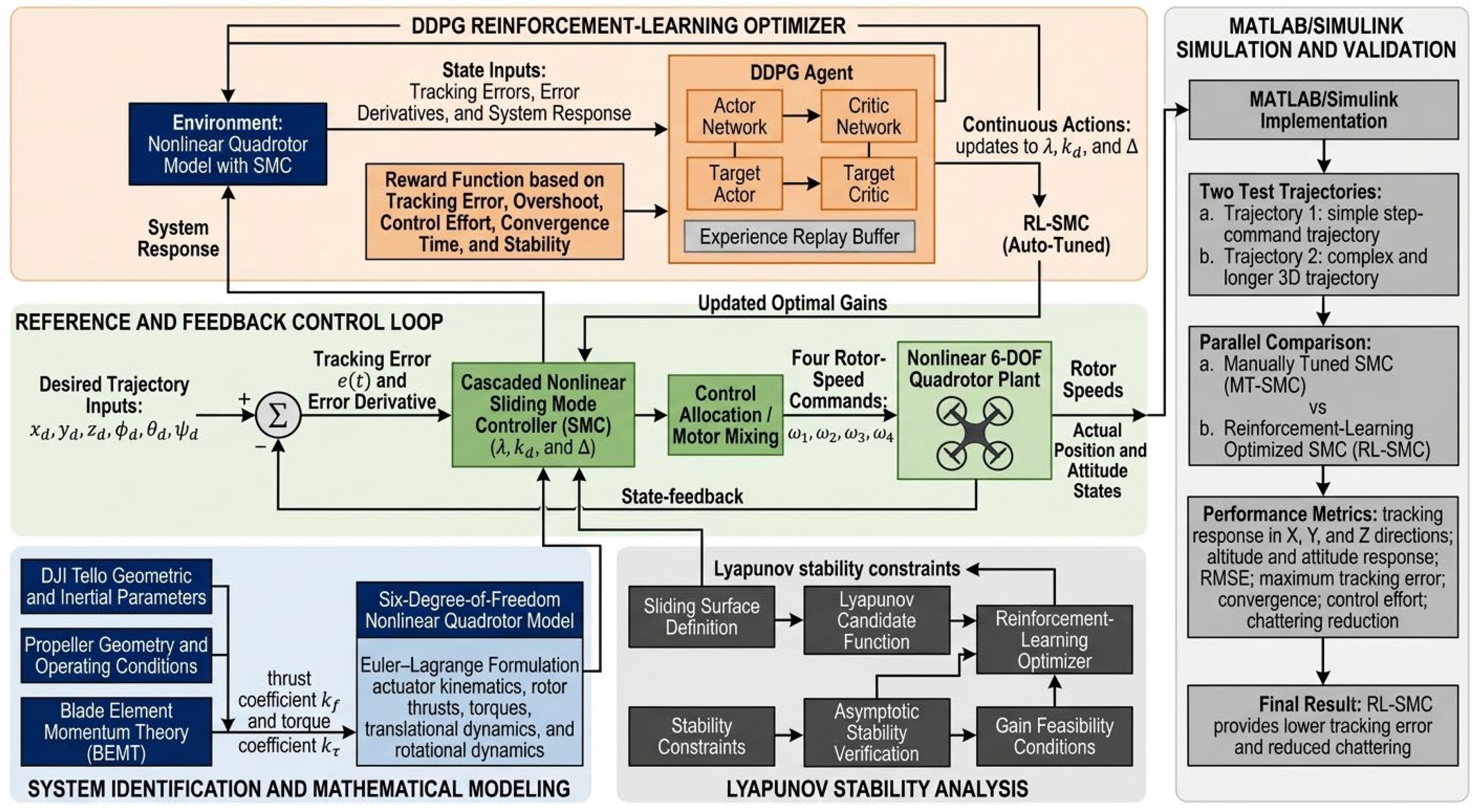
Figure 2.
Quadrotor model with coordinate frame.
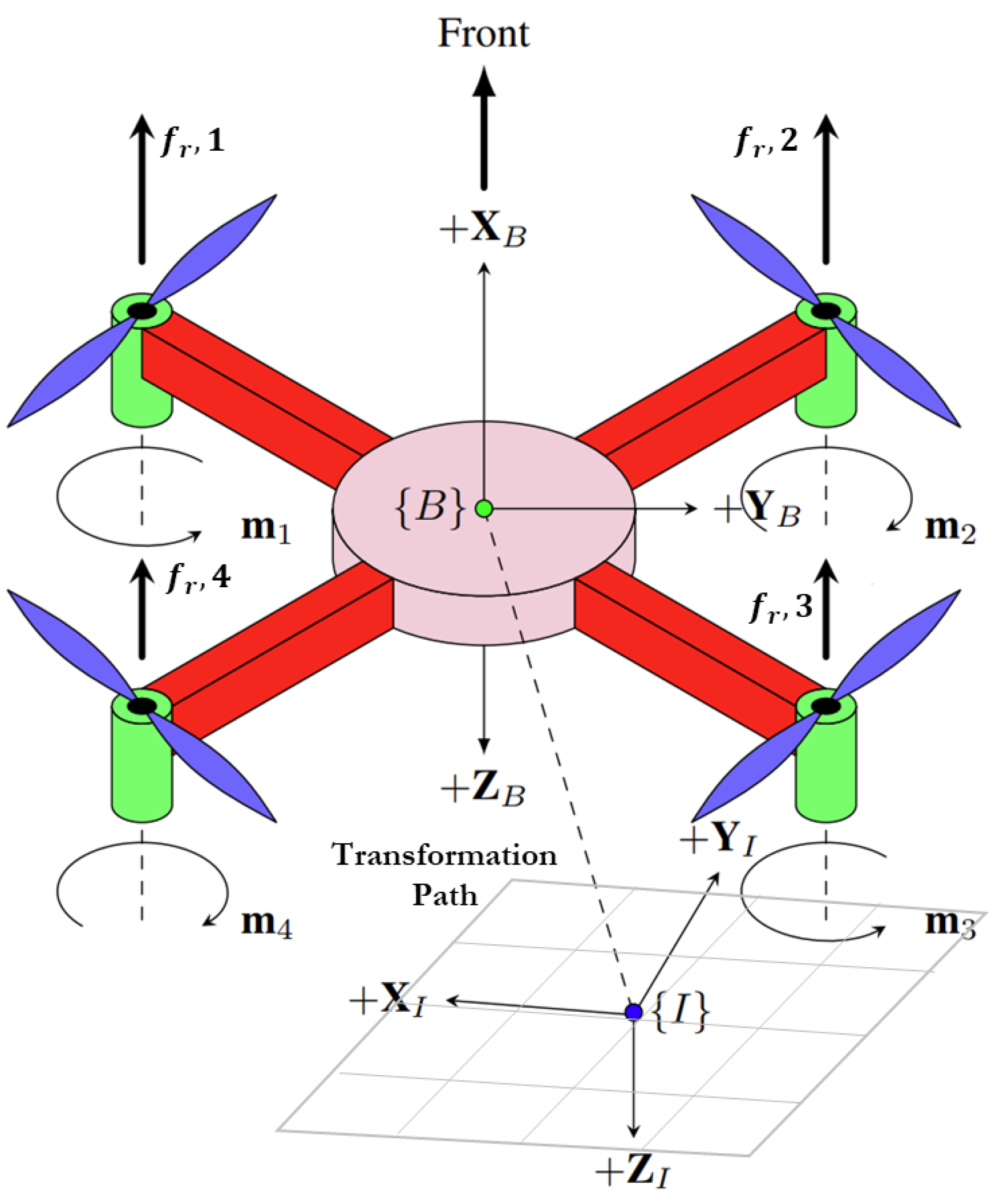
Figure 3.
Deep deterministic policy gradient-based reinforcement learning architecture.
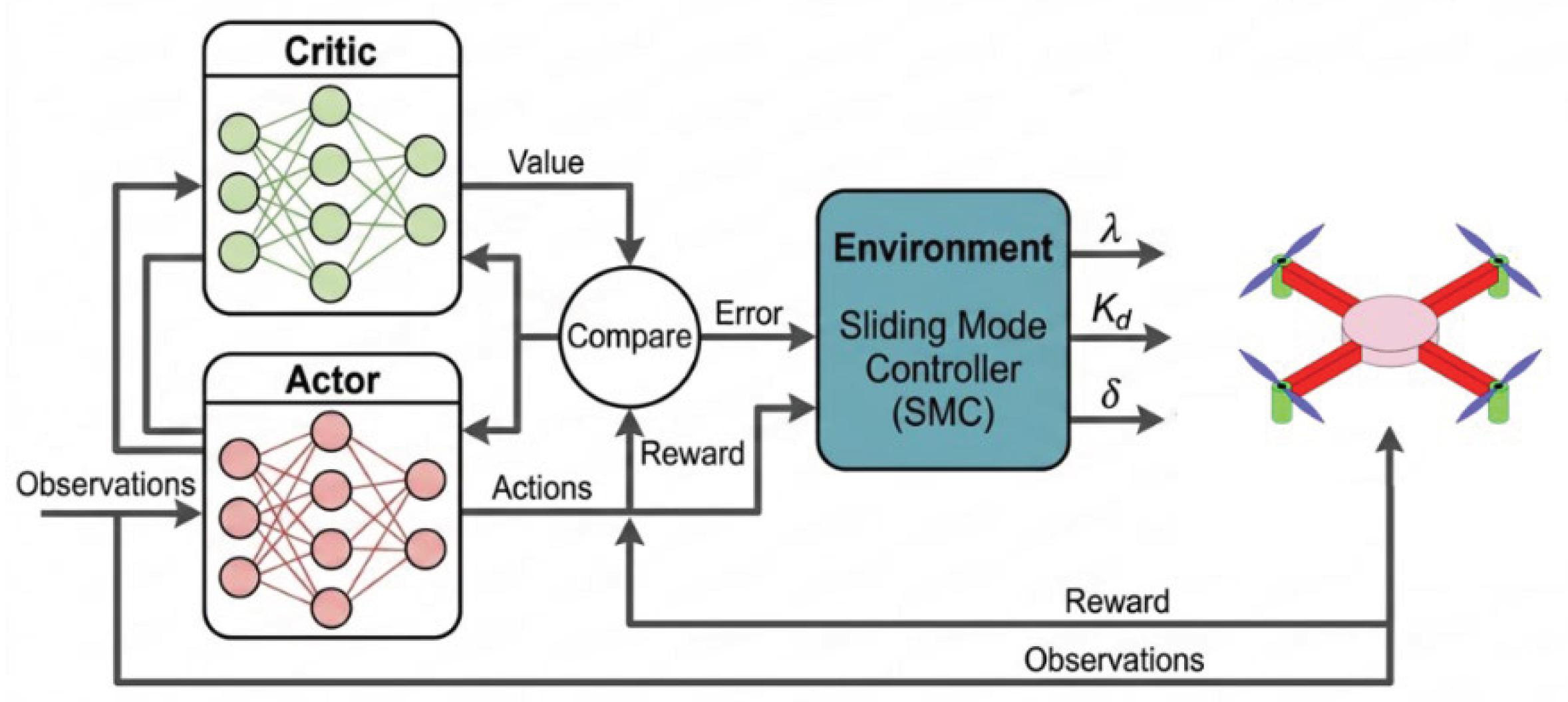
Figure 4.
Quadrotor trajectory comparison in X, Y, Z directions for trajectory 1.
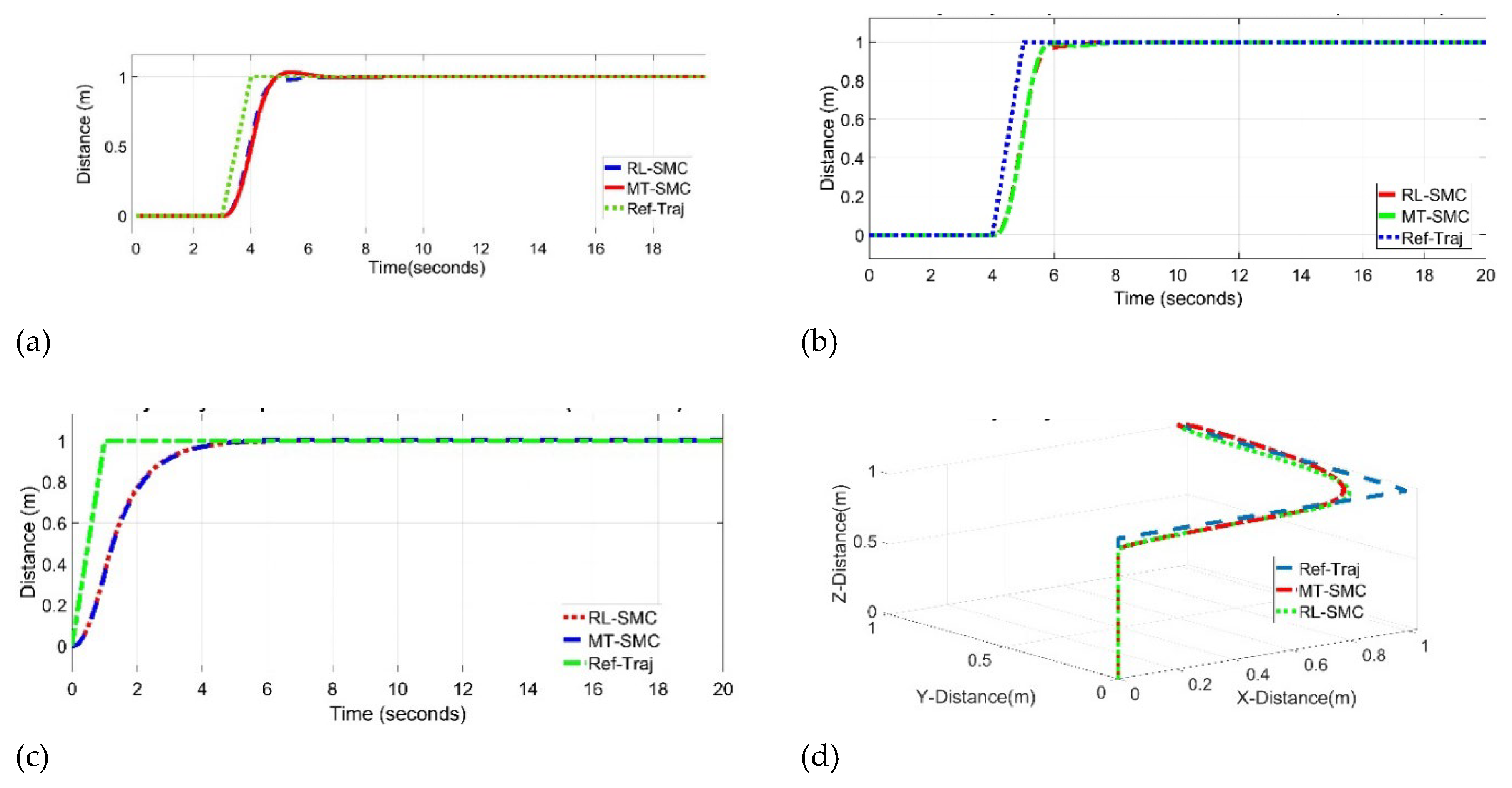
Figure 5.
Error comparison plots in X, Y, Z directions for trajectory 1.
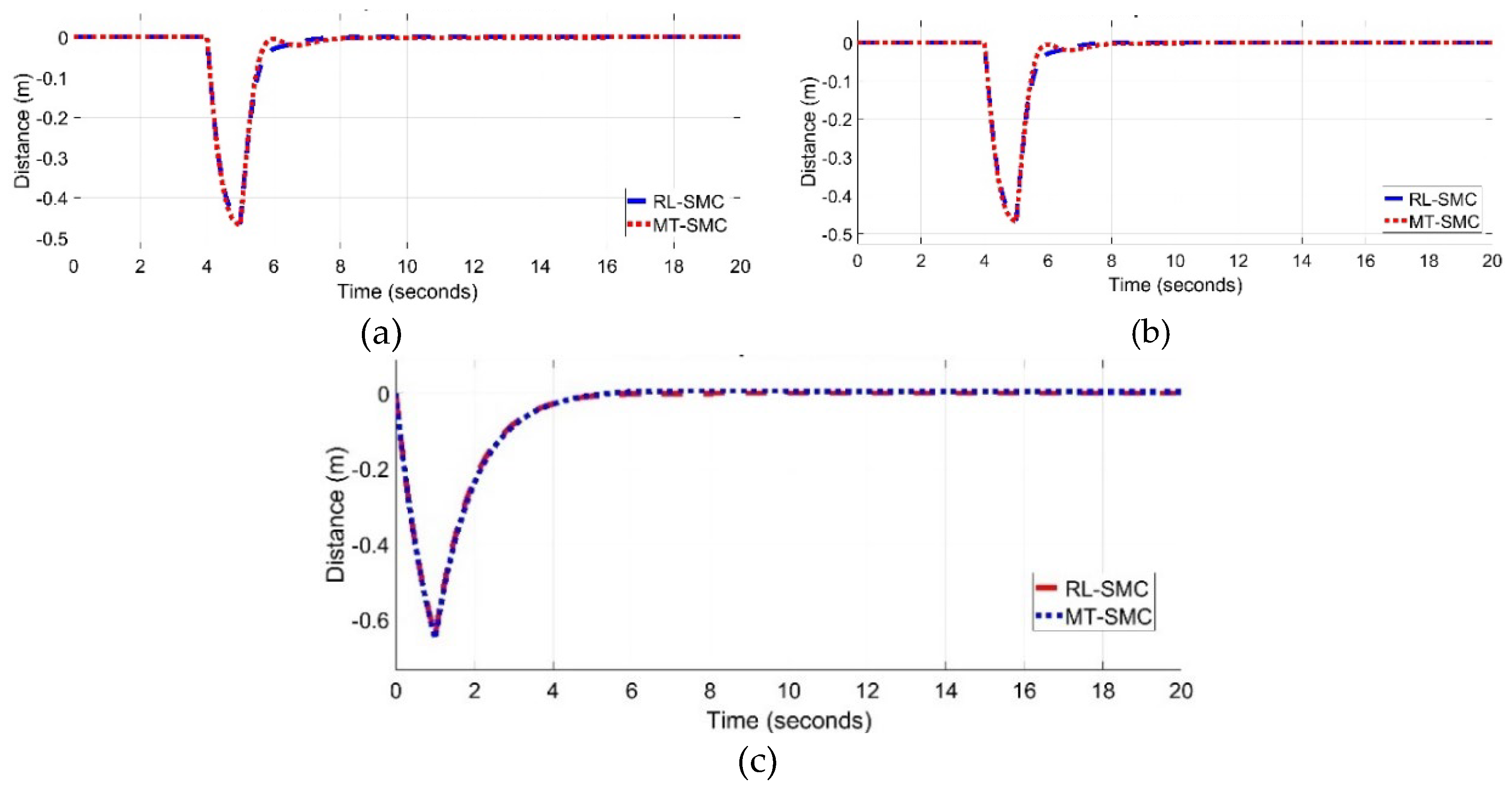
Figure 6.
Quadrotor trajectory comparison in X, Y, Z directions for trajectory 2.
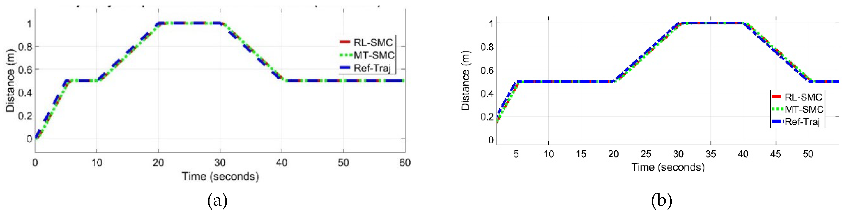
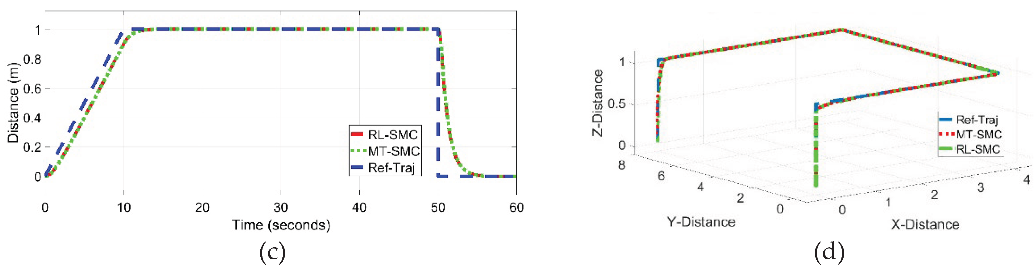
Figure 7.
Error comparison plots in X, Y, Z directions for trajectory 2.
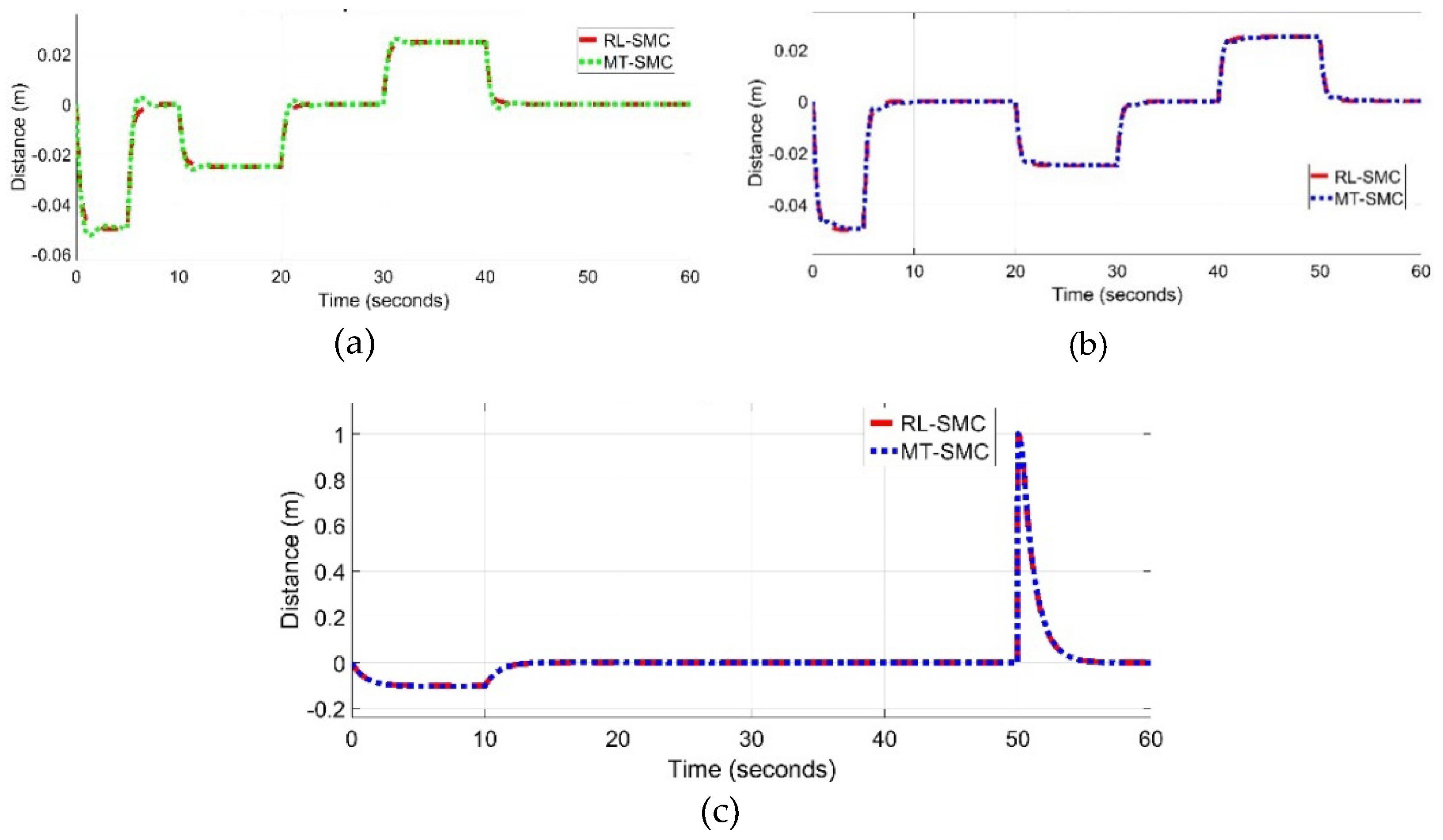

Table 1.
Manual VS Optimal Gain.
| Controller | Manually Tuned Gains | Auto-Tuned Optimal Gains | ||||
|---|---|---|---|---|---|---|
| 3.87 | -3.44 | 5 | 3.278 | -4.17 | 4.69 | |
| 2.8 | -1.1 | 6.5 | 2.2 | -1.46 | 5.87 | |
| 2.0 | -0.90 | 5.0 | 2.48 | -1.04 | 5.6 | |
| 3.07 | -3.14 | 3.94 | 3.78 | -5.17 | 3.76 | |
| 3.4 | -2.0 | 5 | 4.11 | -1.83 | 5.69 | |
| 3.0 | -1.50 | 6.0 | 3.48 | -2.04 | 6.26 | |
Table 2.
Performance of manual and auto-tuned controllers.
| Trajectory | Root Mean Squared Error | Maximum Error | ||||
|---|---|---|---|---|---|---|
| Manual Tuning | Auto Tuning | %age reduction | Manual Tuning | Auto Tuning | %age reduction | |
| 0.1953 | 0.1825 | 6.6 | 0.5 | 0.43 | 14.0 | |
| 0.2939 | 0.2625 | 10.6 | 0.46 | 0.41 | 5.0 | |
| 0.2498 | 0.2412 | 3.44 | 0.65 | 0.61 | 4.0 | |
| 0.1953 | 0.1825 | 6.6 | 0.055 | 0.049 | 10 | |
| 0.2939 | 0.2625 | 10.6 | 0.046 | 0.041 | 10.4 | |
| 0.2498 | 0.2412 | 3.44 | 0.9977 | 0.9520 | 4.57 | |
Disclaimer/Publisher’s Note: The statements, opinions and data contained in all publications are solely those of the individual author(s) and contributor(s) and not of MDPI and/or the editor(s). MDPI and/or the editor(s) disclaim responsibility for any injury to people or property resulting from any ideas, methods, instructions or products referred to in the content. |
© 2026 by the authors. Licensee MDPI, Basel, Switzerland. This article is an open access article distributed under the terms and conditions of the Creative Commons Attribution (CC BY) license (http://creativecommons.org/licenses/by/4.0/).
Copyright: This open access article is published under a Creative Commons CC BY 4.0 license, which permit the free download, distribution, and reuse, provided that the author and preprint are cited in any reuse.