Dynamical Formation of Born Equilibrium and the M-Event Fingerprint

1. Equilibrium and Event Transport

A probability law can be invariant under dynamical evolution without attracting ensembles prepared away from it. This distinction separates the form of the Born rule from the dynamical formation of a Born ensemble. The quantum state and the implemented observation specify the outcome weights [1]; an event-level dynamics must determine how a population comes to occupy those weights. Pilot-wave studies approach this problem through the relaxation of particle distributions, while Nelson dynamics approaches it through stochastic trajectories [2,3].

The physical–observation dual-axis structure places the physical state x and the observation state s at a common record-forming interface [4]. In its M-event realization, a selector phase identifies one event cell, whose Haar volume equals the corresponding Born weight [5]. The phase connection carries the selector through a sequence of interfaces. A closed cycle may return the response to its starting point while retaining a phase fingerprint of its path. Pure phase transport is nevertheless a circle translation: it preserves the Haar distribution and every nonuniformity translated with it. Selective reset contracts response deviations while retaining this phase direction [6]. Equilibrium formation therefore belongs to the population dynamics of the complete cycle.

The central issue is which part of a cycle fluctuation remains unpredictable after the response has been resolved. A reservoir can perturb both response and phase, and their correlated motion can store information in the response that a phase histogram alone conceals. The appropriate equilibrium is consequently conditional: the selector must be Haar distributed at each resolved response, not only after different responses have been averaged together.

We establish that equilibrium and determine its formation rate for a fixed-charge, affine Gaussian return. The contracting response admits an exact phase correction, closely related to asymptotic phase in oscillator noise theory [7]. After this correction, each cycle adds a single independent innovation. Its variance gives a necessary and sufficient condition for attraction from arbitrary initial joint distributions, including singular and phase–response-correlated preparations. Gaussian conditioning gives a finite-time bound at almost every resolved response.

The same innovation determines the M-event fingerprint. A prepared phase harmonic and the matching two-time correlation evolve with the same multiplier. Ensemble formation and fingerprint decay thus become linked predictions of one cycle law. We carry this relation through variable-width event readout, a two-stage preparation protocol, and finite-time perturbations of the implemented instrument. The Born cell geometry supplies the target weights; the open-cycle dynamics determines their populations and the correlations between successive events.

2. The Joint Ensemble and Its Reservoir-Coupled Cycle

2.1. Conditional Event Populations

Let z denote the resolved response at a fixed physical control endpoint. A finite outcome family has measurable selector cells $C_y\left(z\right)\subset \mathbb{T}$, where $\mathbb{T}=\mathbb{R}/\left(2\pi \mathbb{Z}\right)$, and

$${\mu }_{\mathrm{H}}\left[C_y\left(z\right)\right]=K_y\left(z\right),{\mu }_{\mathrm{H}}\left(\mathrm{d}\chi \right)={\displaystyle \frac{\mathrm{d}\chi }{2\pi }}.$$

(1)

Here $K_y\left(z\right)$ is the Born kernel of the interface. A joint ensemble $\mu \left(\mathrm{d}z\mathrm{d}\chi \right)$ gives

$$p_{\mu }(y\mid z)=\mu [C_y\left(z\right)\mid z].$$

(2)

The ensemble is conditionally phase-equilibrated when

$$\mu \left(\mathrm{d}z\mathrm{d}\chi \right)={\mu }_z\left(\mathrm{d}z\right){\mu }_{\mathrm{H}}\left(\mathrm{d}\chi \right).$$

(3)

It then has the Born probabilities at almost every resolved interface.

The response label carries essential information. Assign two equally probable labels opposite uniform semicircle distributions of the selector. Their phase mixture is Haar, yet a common balanced cell has conditional probabilities one and zero. The joint factorization in Eq. (3) removes the correlation hidden by that mixture.

The outcome-resolved instrument ${\mathsf{K}}_y$ induces the population kernel

$$\mathsf{P}=\sum _y{\mathsf{K}}_y,{\mu }_{n+1}={\mu }_n\mathsf{P}.$$

(4)

For a phase-covariant cycle, the response transition and the added phase depend on the response and reservoir variables. Its kernel has the form

$$\mathsf{P}[(z,\chi ),\mathrm{d}{z}^{\prime }\mathrm{d}{\chi }^{\prime }]=\int k_z\left(\mathrm{d}{z}^{\prime }\mathrm{d}\delta \right){\delta }_{\chi +{\kappa }_{\mathrm{M}}+\delta }\left(\mathrm{d}{\chi }^{\prime }\right).$$

(5)

Phase translation in the incoming state therefore produces the same translation in the outgoing state.

Proposition 1 

(Invariance of conditional equilibrium). If the response marginal of $k_z$ has invariant law ${\pi }_z$, then $\Pi ={\pi }_z\otimes {\mu }_{\mathrm{H}}$ is invariant under Eq. (5). Every product ${\mu }_z\otimes {\mu }_{\mathrm{H}}$ remains conditionally Haar after a cycle.

Proof. 

For fixed $z,z^{\prime },\delta$, the translation $\chi \mapsto \chi +{\kappa }_{\mathrm{M}}+\delta$ preserves Haar measure. Integrating first over $\chi$ and then over $k_z$ leaves the evolved response law times Haar measure. Choosing ${\mu }_z={\pi }_z$ proves invariance. □

The proposition allows a common reservoir to correlate the response kick and the phase kick. Attraction requires the dynamics of those kicks, which we now specify.

2.2. Action, Response, and Return

On the regular binary chart, the response–selector action is [5]

$$S_0=\int \left\{{\displaystyle \frac{{\mathcal{I}}_S}{2}}{\dot{\vartheta }}^2+q_{\chi }\left[\dot{\chi }-{\displaystyle \frac{1-cos\vartheta }{2}}\dot{\phi }\right]\right\}\mathrm{d}t.$$

(6)

The physical azimuth is driven by $\phi \left(u\right)=Xcosu$, with $u=\Omega t$, $X=0.100$, and $q_{\chi }/\left({\mathcal{I}}_S\Omega \right)=4$. The balanced observation response satisfies

$${\vartheta }_{*}^{\prime \prime }=0.2sin{\vartheta }_{*}sinu,{\vartheta }_{*}\left(0\right)={\vartheta }_{*}\left(2\pi \right)={\displaystyle \frac{\pi }{2}}.$$

(7)

Its periodic solution starts at $v_{*}=-0.1974174831341\dots$ and transports the selector through the phase

$${\kappa }_{\mathrm{M}}=0.03080966336634\dots .$$

(8)

These quantities specify the reference cycle.

At fixed $q_{\chi }$, write $\xi ={(\vartheta -\pi /2,v-v_{*})}^{\mathsf{T}}$. An isotropic meridional reset attenuates the response by a and contributes zero selector phase. The response Jacobian and drive-phase gradient are [6]

$$\begin{array}{cc}\hfill B& =aM,M=\left(\begin{array}{cc}1.411751160170& 7.192815523855\\ 0.138060170589& 1.411751160170\end{array}\right),\hfill \\ \hfill h& =\left(\begin{array}{c}0.019806668385\\ 0.345999539570\end{array}\right).\hfill \end{array}$$

(9)

The linear return is ${\xi }^{\prime }=B\xi$, ${\chi }^{\prime }=\chi +{\kappa }_{\mathrm{M}}+h^{\mathsf{T}}\xi$. Its response is stable for $0<a<0.415236565073\dots$. The angle $\vartheta$ remains an observation-response coordinate; the selector and its conjugate charge belong to the event layer over the physical–observation interface.

2.3. Canonical Reservoir Impulses

Each completed return is followed by a reservoir impulse. In the meridional chart, $p_{\vartheta }={\mathcal{I}}_S\Omega v$ is conjugate to $\vartheta$, and $q_{\chi }$ is conjugate to $\chi$. The integrated generator

$$F_n=p_{\vartheta }{\zeta }_{\vartheta ,n}-{\mathcal{I}}_S\Omega \vartheta {\zeta }_{v,n}+q_{\chi }{\eta }_n$$

(10)

produces

$$(\vartheta ,v,\chi ,q_{\chi })\mapsto (\vartheta +{\zeta }_{\vartheta ,n},v+{\zeta }_{v,n},\chi +{\eta }_n,q_{\chi }).$$

(11)

Its system Hamiltonian vector field is constant. The translation is therefore exact at finite integrated kick, and the selector charge is conserved. The kick variables can be represented as commuting momenta of reservoir canonical pairs: they remain constant during the impulse, while their conjugate coordinates receive its backaction. Fresh preparation fixes their joint law before the next cycle.

Averaging over these reservoir variables gives the affine return on ${\mathbb{R}}^d\times \mathbb{T}$,

$$\begin{array}{cc}\hfill {\xi }_{n+1}& =B{\xi }_n+{\zeta }_n,\hfill \\ \hfill {\chi }_{n+1}& ={\chi }_n+{\kappa }_{\mathrm{M}}+h^{\mathsf{T}}{\xi }_n+{\eta }_n(mod2\pi ).\hfill \end{array}$$

(12)

We use a general response dimension d in the analysis. The increments $({\zeta }_n,{\eta }_n)$ are identically distributed centered Gaussians, independent across cycles and of the initial joint state, with covariance

$$\mathsf{C}=\left(\begin{array}{cc}Q& c\\ c^{\mathsf{T}}& {\sigma }_{\eta }^2\end{array}\right)⪰0.$$

(13)

The response is Schur stable, $\rho \left(B\right)<1$, and controllable by its reservoir,

$${span}_{0\le j<d}range\left(B^j{Q}^{1/2}\right)={\mathbb{R}}^d.$$

(14)

Consequently, its stationary covariance is positive definite and satisfies

$$S=BS{B}^{\mathsf{T}}+Q.$$

(15)

Equations (12)–(14) define the realization studied below. The reservoir covariance describes the coupling and preparation of the open cycle, as in Gaussian relaxation theory [8]. Preparation contains no intermediate selector-sensitive readout. Fingerprint measurements use a specified subsequent instrument, with the pair-transparent return of Ref. [6] providing the reference case. Section 8 gives quantitative bounds for nonlinear response and readout recoil.

3. The Phase Carried beyond a Response Transient

A response displacement produces phase over all later cycles in which it persists. Stability makes their sum finite:

$${\displaystyle \sum _{j=0}^{\infty }}{h}^{\mathsf{T}}{B}^j\xi ={\ell }^{\mathsf{T}}\xi ,\ell ={(I-B^{\mathsf{T}})}^{-1}h.$$

(16)

This suggests the corrected phase

$$\psi =\chi +{\ell }^{\mathsf{T}}\xi (mod2\pi ).$$

(17)

It includes the future phase of the unforced response. With reservoir increments present, it separates an accumulated innovation from an endpoint difference, the explicit finite-dimensional form of an innovation–coboundary decomposition [9].

Theorem 1 

(Exact phase reduction). The return in Eq. (12) obeys

$$\begin{array}{cc}\hfill {\psi }_{n+1}& ={\psi }_n+{\kappa }_{\mathrm{M}}+{ϵ}_n(mod2\pi ),\hfill \\ \hfill {ϵ}_n& ={\eta }_n+{\ell }^{\mathsf{T}}{\zeta }_n.\hfill \end{array}$$

(18)

The innovations are independent centered Gaussians with variance

$$D={\sigma }_{\eta }^2+2{\ell }^{\mathsf{T}}c+{\ell }^{\mathsf{T}}Q\ell \ge 0.$$

(19)

Proof. 

Substitution of Eq. (12) into Eq. (17) cancels the response term because $h^{\mathsf{T}}+{\ell }^{\mathsf{T}}B={\ell }^{\mathsf{T}}$. The remaining increment is the stated linear combination of the reservoir variables, whose variance is Eq. (19). □

On a real lift of the phase path,

$${\chi }_n-{\chi }_0-n{\kappa }_{\mathrm{M}}={\displaystyle \sum _{j=0}^{n-1}}{ϵ}_j-{\ell }^{\mathsf{T}}({\xi }_n-{\xi }_0).$$

(20)

At response stationarity the endpoint term has bounded variance. The innovations, in contrast, contribute $nD$. This decomposition identifies the phase fluctuation that survives the decay of response transients.

Proposition 2 

(Invariance under a response-frame change). Under $\tilde{\chi }=\chi +L^{\mathsf{T}}\xi$, with the event-cell reference translated by the same amount, both the corrected phase and D are unchanged.

Proof. 

The transformed coefficients are $\tilde{h}=h+(B^{\mathsf{T}}-I)L$, $\tilde{\eta }=\eta +L^{\mathsf{T}}\zeta$, and $\tilde{\ell }=\ell -L$. Thus $\tilde{\chi }+{\tilde{\ell }}^{\mathsf{T}}\xi =\psi$ and $\tilde{\eta }+{\tilde{\ell }}^{\mathsf{T}}\zeta =ϵ$. □

A response-dependent translation also preserves conditional Haar measure. The variables $\psi$ and $\chi$ therefore express the same conditional equilibrium, while the experimental event continues to be read from its calibrated cell.

4. Formation of Conditional Born Equilibrium

The corrected phase is a circle random walk. Its correlation with the final response contains the remaining information needed to determine the ensemble at a resolved interface. For $n\ge d$, define

$$\begin{array}{cc}\hfill S_n& ={\displaystyle \sum _{j=0}^{n-1}}{B}^{j}Q{\left(B^{\mathsf{T}}\right)}^j=S-B^{n}S{\left(B^{\mathsf{T}}\right)}^n,\hfill \\ \hfill w& =Q\ell +c,r_n={\displaystyle \sum _{j=0}^{n-1}}{B}^{j}w,\hfill \\ \hfill v_n& =nD-r_n^{\mathsf{T}}{S}_n^{-1}{r}_n.\hfill \end{array}$$

(21)

Controllability gives $S_n\succ 0$. The same definitions apply at any earlier n for which $S_n$ is invertible.

Lemma 1 

(Phase distribution at a resolved response). Starting from a fixed $({\xi }_0,{\psi }_0)$ and a real lift of ${\psi }_0$, the vector $({\xi }_n,{\psi }_n-n{\kappa }_{\mathrm{M}})$ is Gaussian with covariance blocks $S_n$, $r_n$, and $nD$. Conditional on ${\xi }_n$, its phase variance is $v_n$ and its phase mean is

$${\psi }_0+n{\kappa }_{\mathrm{M}}+r_n^{\mathsf{T}}{S}_n^{-1}({\xi }_n-B^n{\xi }_0).$$

(22)

Proof. 

Iteration gives

$$\begin{array}{cc}\hfill {\xi }_n& =B^n{\xi }_0+{\displaystyle \sum _{j=0}^{n-1}}{B}^{n-1-j}{\zeta }_j,\hfill \\ \hfill {\psi }_n& ={\psi }_0+n{\kappa }_{\mathrm{M}}+{\displaystyle \sum _{j=0}^{n-1}}{ϵ}_j.\hfill \end{array}$$

Since $Cov({\zeta }_j,{ϵ}_j)=w$, their cross covariance is $r_n$. Gaussian conditioning gives the mean and the nonnegative Schur-complement variance in Eq. (21). □

Thus $v_n$ is the phase dispersion left after the final response has been observed. For $v>0$ let

$$\epsilon \left(v\right)=min\left\{1,{\left[{\displaystyle \frac{1}{2}}{\displaystyle \sum _{m=1}^{\infty }}{e}^{-m^{2}v}\right]}^{1/2}\right\},\epsilon \left(0\right)=1.$$

(23)

Total variation is normalized to lie in $[0,1]$.

Theorem 2 

(Conditional equilibration). For the cycle in Eqs. (12)–(14), let ${\mu }_0$ be any initial probability law independent of the reservoir sequence. Whenever $S_n\succ 0$,

$$TV[{\mu }_n(\mathrm{d}\chi \mid \xi ),{\mu }_{\mathrm{H}}]\le \epsilon \left(v_n\right)$$

(24)

for ${\left({\mu }_n\right)}_{\xi }$-almost every ξ, and

$${\delta }_n^{\mathrm{cond}}:=TV[{\mu }_n,{\left({\mu }_n\right)}_{\xi }\otimes {\mu }_{\mathrm{H}}]\le \epsilon \left(v_n\right).$$

(25)

The condition $D>0$ is necessary and sufficient for attraction from every initial joint law to

$$\Pi =\mathcal{N}(0,S)\otimes {\mu }_{\mathrm{H}}.$$

(26)

When $D>0$, Π is the unique invariant law, ${\mu }_n\to \Pi$ in total variation, and the conditional bound decays as $O\left(e^{-nD/2}\right)$.

Proof. 

A Gaussian of variance v wrapped onto the circle has Fourier coefficients of modulus $e^{-m^{2}v/2}$. Parseval’s identity and Cauchy–Schwarz, relative to Haar measure, yield

$$TV({\mathcal{W}}_v,{\mu }_{\mathrm{H}})\le {\displaystyle \frac{1}{2}}{\left(2\sum _{m\ge 1}{e}^{-m^{2}v}\right)}^{1/2}.$$

(27)

The bound is independent of the Gaussian mean. Apply it to the conditional law in the lemma. For an arbitrary initial distribution, the phase law at a fixed final response is a posterior mixture of these wrapped Gaussians, all with variance $v_n$. Convexity gives Eq. (24). Integration over the response gives Eq. (25).

Stability implies that $r_n$ is bounded and $S_n\to S\succ 0$, so

$$v_n=nD-O\left(1\right).$$

(28)

For $D>0$, Eq. (23) is therefore $O\left(e^{-nD/2}\right)$. From each fixed response point, $\mathcal{N}(B^n{\xi }_0,S_n)$ converges in total variation to $\mathcal{N}(0,S)$. Its distance is bounded by one; dominated convergence extends the result to any initial response law. Combining marginal convergence with Eq. (25) proves ${\mu }_n\to \Pi$. Applying this convergence to any invariant initial law proves uniqueness.

For $D=0$, ${ϵ}_n=0$ almost surely. Choose a preparation with fixed ${\psi }_0$. At every cycle its joint state is supported on

$$\chi ={\psi }_0+n{\kappa }_{\mathrm{M}}-{\ell }^{\mathsf{T}}\xi (mod2\pi ).$$

(29)

This graph has zero measure under any response law times Haar measure. Its conditional distance is one, so attraction from all preparations fails. □

Response controllability supplies smoothing in the response coordinates; the positive innovation variance supplies mixing in the phase. Together they establish equilibrium at each resolved interface. The conditional estimate is uniform over preparations, including point masses and correlations between the initial phase and response.

Corollary 1 

(Optimal conditional formation rate). Let $D>0$ and $S_n\succ 0$. A preparation concentrated at one corrected phase satisfies

$${\displaystyle \frac{1}{2}}{e}^{-nD/2}\le {\delta }_n^{\mathrm{cond}}\le \epsilon \left(v_n\right).$$

(30)

The rate $D/2$ is therefore optimal among exponential bounds valid for every initial preparation.

Proof. 

The expectation of $e^{\mathrm{i}{\psi }_n}$ has modulus $e^{-nD/2}$ by Eq. (18); under ${\left({\mu }_n\right)}_{\xi }\otimes {\mu }_{\mathrm{H}}$ it is zero. A unit-modulus test function bounds this difference by $2{\delta }_n^{\mathrm{cond}}$. The upper bound is Theorem 2. □

The response marginal has its own approach to stationarity. Equation (30) identifies the rate of conditional phase formation itself.

Corollary 2 

(Conditional Born probabilities). For every finite event partition in Eq. (1),

$${\displaystyle \frac{1}{2}}\sum _y\left|p_{{\mu }_n}(y\mid \xi )-K_y\left(\xi \right)\right|\le \epsilon \left(v_n\right)$$

(31)

for ${\left({\mu }_n\right)}_{\xi }$-almost every ξ. The same bound holds after averaging over the response.

Proof. 

The event map sends a phase to its cell. Total variation contracts under this measurable map; apply Eq. (24). □

The event geometry remains fixed while its populations approach the Born weights. Equations (21) and (31) quantify that approach using the cycle parameters alone.

4.1. Correlated Kicks and the Zero-Innovation State

The transition at $D=0$ can occur with a noisy response and a noisy recorded phase. Consider

$${\eta }_n=-t{\ell }^{\mathsf{T}}{\zeta }_n,{\zeta }_n\sim \mathcal{N}(0,Q).$$

(32)

Their separate phase variance and persistent innovation variance are

$$Var{\eta }_n=t^2{\ell }^{\mathsf{T}}Q\ell ,D={(1-t)}^2{\ell }^{\mathsf{T}}Q\ell .$$

(33)

At $t=1$, the corrected phase rotates rigidly and all raw phase fluctuation is carried by the endpoint term in Eq. (20). The response therefore retains exactly the information needed to recover the phase label.

An independent residual kick of variance ${\sigma }_{\mathrm{res}}^2$ changes the persistent variance to $D={(1-t)}^2{\ell }^{\mathsf{T}}Q\ell +{\sigma }_{\mathrm{res}}^2$. It sets the decay rate of the formerly conserved mode. Separate measurements of the two raw variances leave this rate undetermined; their cross covariance completes the prediction.

5. One Spectrum for Formation and the Fingerprint

Equilibration follows the decay of an ensemble’s prepared modes. A fingerprint follows a phase difference along one history. The corrected phase places both observables under the same cycle operator.

Theorem 3 

(Formation–fingerprint identity). For a nonzero integer m, define

$$\begin{array}{cc}\hfill A_m\left(n\right)& =\mathbb{E}{e}^{\mathrm{i}m({\psi }_n-n{\kappa }_{\mathrm{M}})},\hfill \\ \hfill F_m\left(n\right)& =\mathbb{E}{e}^{\mathrm{i}m({\psi }_n-{\psi }_0-n{\kappa }_{\mathrm{M}})}.\hfill \end{array}$$

(34)

For every initial joint law independent of future reservoir increments,

$$A_m\left(n\right)=A_m\left(0\right)e^{-m^{2}nD/2},F_m\left(n\right)=e^{-m^{2}nD/2}.$$

(35)

The backward cycle operator has eigenfunction $e^{\mathrm{i}m\psi }$ and eigenvalue

$${\lambda }_m=e^{\mathrm{i}m{\kappa }_{\mathrm{M}}-m^{2}D/2}.$$

(36)

Proof. 

After n cycles the corrected phase advances by $n{\kappa }_{\mathrm{M}}+{\sum }_{j<n}{ϵ}_j$. The independent Gaussian sum has characteristic function $e^{-m^{2}nD/2}$. Averaging with or without the initial phase factor gives Eq. (35). Conditioning on the initial state for one cycle gives Eq. (36). □

Thus the harmonic rates are

$${\gamma }_m=-log\left|{\lambda }_m\right|={\displaystyle \frac{m^{2}D}{2}}.$$

(37)

For $A_m\left(0\right)\ne 0$, the normalized preparation mode satisfies $A_m\left(n\right)/A_m\left(0\right)=F_m\left(n\right)$. A fixed channel attenuates both by exactly the same factor at equal lag. The rate is indexed by the same harmonic: a preparation with no first mode can relax faster in a selected observable, while response observables retain their own modes.

An equilibrium ensemble has $A_m\left(0\right)=0$ for every $m\ne 0$, whereas its finite-lag $F_m\left(n\right)$ remains nonzero. Born equilibrium and a temporal fingerprint therefore coexist. Equation (35) determines how that fingerprint decays, as well as how an initially populated mode disappears. For independent response and phase kicks, $c=0$, Eq. (19) reduces to the long-run phase-variance coefficient $D_{\mathrm{eff}}$ of Ref. [6].

For identically distributed independent innovations beyond the Gaussian family, the exact phase reduction gives $A_m\left(n\right)=A_m\left(0\right)\phi {\left(m\right)}^n$ and $F_m\left(n\right)=\phi {\left(m\right)}^n$, where $\phi \left(m\right)=\mathbb{E}{e}^{\mathrm{i}m{ϵ}_n}$. Their common spectrum remains intact. Gaussianity specifies $\phi \left(m\right)=e^{-m^{2}D/2}$ and makes the conditional phase law explicitly soluble.

5.1. The Fingerprint Read by the Event Cells

The event cells use $\chi$. In the stationary response ensemble with initial Haar phase independent of the response and future increments, the recorded phase fluctuation has variance

$$\begin{array}{cc}\hfill V_n^{\chi }=& nD+{\ell }^{\mathsf{T}}[2S-B^{n}S-S{\left(B^{\mathsf{T}}\right)}^n]\ell \hfill \\ \hfill & -2{\ell }^{\mathsf{T}}{r}_n.\hfill \end{array}$$

(38)

Appendix A derives the identity. It includes the response endpoint term and correlations within each reservoir kick. For transparent readout of the balanced event $Y_n=sgncos{\chi }_n$,

$$\begin{array}{cc}\hfill C_n:=\mathbb{E}\left(Y_0{Y}_n\right)& ={\displaystyle \frac{8}{{\pi }^2}}\sum _{\begin{array}{c}m\ge 1\\ m\mathrm{odd}\end{array}}{\displaystyle \frac{cos\left(mn{\kappa }_{\mathrm{M}}\right)}{m^2}}{e}^{-m^2{V}_n^{\chi }/2},\hfill \\ \hfill P_{\mathrm{mis}}\left(n\right)& ={\displaystyle \frac{1-C_n}{2}}.\hfill \end{array}$$

(39)

Haar averaging of the two event indicators retains equal Fourier indices. Their squared coefficients are $4/\left({\pi }^2{m}^2\right)$ at each nonzero odd index, giving Eq. (39) [6]. The response endpoints change finite-lag amplitudes; the relation $V_n^{\chi }=nD+O\left(1\right)$ retains the harmonic envelope exponents. The conditional formation theorem determines how closely a prepared ensemble approaches the stationary initial law used here.

6. Reading Equilibrium from Event Populations

Each event partition selects a family of phase modes. Let its positive cell be the arc centered at $\beta$ with length $2\pi p$, and set $a_m=\mathbb{E}{e}^{\mathrm{i}m\chi }$. For an integrable phase density,

$$p_{+}(p,\beta )-p=2\sum _{m\ge 1}{\displaystyle \frac{sin\left(m\pi p\right)}{m\pi }}Re\left[a_m{e}^{-\mathrm{i}m\beta }\right].$$

(40)

The series is interpreted in the Fejér sense; convolution with the interval indicator gives the arc probability. At $p=1/2$, every even mode vanishes from the measurement.

Proposition 3 

(Phase modes invisible to balanced cells). For $0<\left|b\right|\le 1$, the density relative to Haar measure

$$\rho \left(\chi \right)=1+bcos2\chi$$

(41)

assigns probability $1/2$ to every semicircle. A quarter-circle cell gives

$$p_{+}(1/4,\beta )={\displaystyle \frac{1}{4}}+{\displaystyle \frac{b}{2\pi }}cos2\beta .$$

(42)

Proof. 

The integral of $cos2\chi$ over any interval of length $\pi$ is zero. Over the centered interval of length $\pi /2$ it is $cos2\beta$. Multiplication by $b/\left(2\pi \right)$ gives Eq. (42). □

A phase scan at a width satisfying $sin\left(m\pi p\right)\ne 0$ for $m=1,\dots ,M$ identifies those Fourier coefficients. The choice $p=1/(M+1)$ meets this condition. For a finite scan, a bandwidth or Fourier-tail estimate controls aliasing. Response-resolved scans retain the conditioning required by Theorem 2. They distinguish a dynamically equilibrated selector from a nonequilibrium distribution that happens to reproduce balanced counts.

7. Equilibrium Preparation Followed by Fingerprint Readout

The common spectral law leads to a separation of tasks. A strongly mixing channel first prepares conditional equilibrium; a quieter channel then retains the stationary ensemble with a longer-lived fingerprint. The two channels may share the response reset and the geometric phase. Their reservoir covariances set the two time scales.

We take $a=0.30$, $Q={10}^{-6}{I}_2$, and $c=0$. Integrating Eq. (7) and its variational equations gives

$$\begin{array}{cc}\hfill \ell & =\left(\begin{array}{c}0.105983711365\\ 0.996914474801\end{array}\right),\hfill \\ \hfill {\ell }^{\mathsf{T}}Q\ell & =1.00507101714\times {10}^{-6}.\hfill \end{array}$$

(43)

The preparation channel uses ${\sigma }_{\eta }=0.2$, and the quiet channel uses ${\sigma }_{\eta }=0.002$. This change affects the phase kick while retaining the small response covariance. Both channels have the same invariant response–Haar law.

Starting from ${\xi }_0=0$ and a fixed selector phase, 350 preparation cycles give

$$\epsilon \left(v_{350}\right)=0.00064468687.$$

(44)

The response distance to its stationary Gaussian is below ${10}^{-90}$ by the estimate in Appendix A. Equation (44) therefore bounds the joint preparation error at the displayed precision. The first-harmonic e-folding times are approximately $50.0$ preparation cycles and $4.00\times {10}^5$ quiet cycles.

Proposition 4 

(Preparation accuracy for a complete future record). Let a prepared joint law have total-variation distance at most δ from Π. Under any common subsequent observation protocol, every event probability differs from its Π-prepared value by at most δ. A correlation with values in $[-1,1]$ differs by at most $2\delta$.

Proof. 

The entire future experiment, including outcome-dependent control, is a Markov kernel from the prepared state to the record. Total variation contracts under that kernel. Testing an event indicator gives the first bound; testing a bounded signed observable gives the second. □

The error estimate therefore passes from preparation to the full fingerprint, rather than only to the next marginal.

Figure 1. Formation of conditional equilibrium for $a=0.30$, $Q={10}^{-6}{I}_2$, $c=0$, and ${\sigma }_{\eta }=0.2$. Phase modes start from a fixed corrected phase. The bound $\epsilon \left(v_n\right)$ applies to arbitrary initial joint distributions. The curves are calculated from the Gaussian cycle.

Figure 1. Formation of conditional equilibrium for $a=0.30$, $Q={10}^{-6}{I}_2$, $c=0$, and ${\sigma }_{\eta }=0.2$. Phase modes start from a fixed corrected phase. The bound $\epsilon \left(v_n\right)$ applies to arbitrary initial joint distributions. The curves are calculated from the Gaussian cycle.

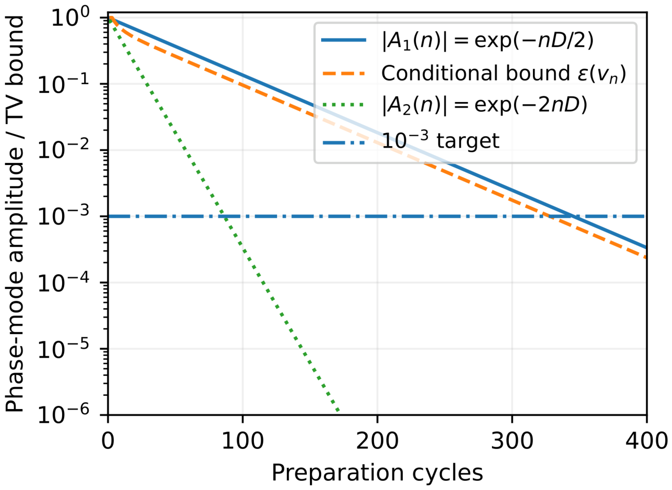
Figure 2. Cancellation of persistent innovation by correlated kicks. At $t=1$, $D=0$ although the raw phase-kick variance is positive. The dotted curve adds an independent residual standard deviation $2\times {10}^{-4}$.

Figure 2. Cancellation of persistent innovation by correlated kicks. At $t=1$, $D=0$ although the raw phase-kick variance is positive. The dotted curve adds an independent residual standard deviation $2\times {10}^{-4}$.

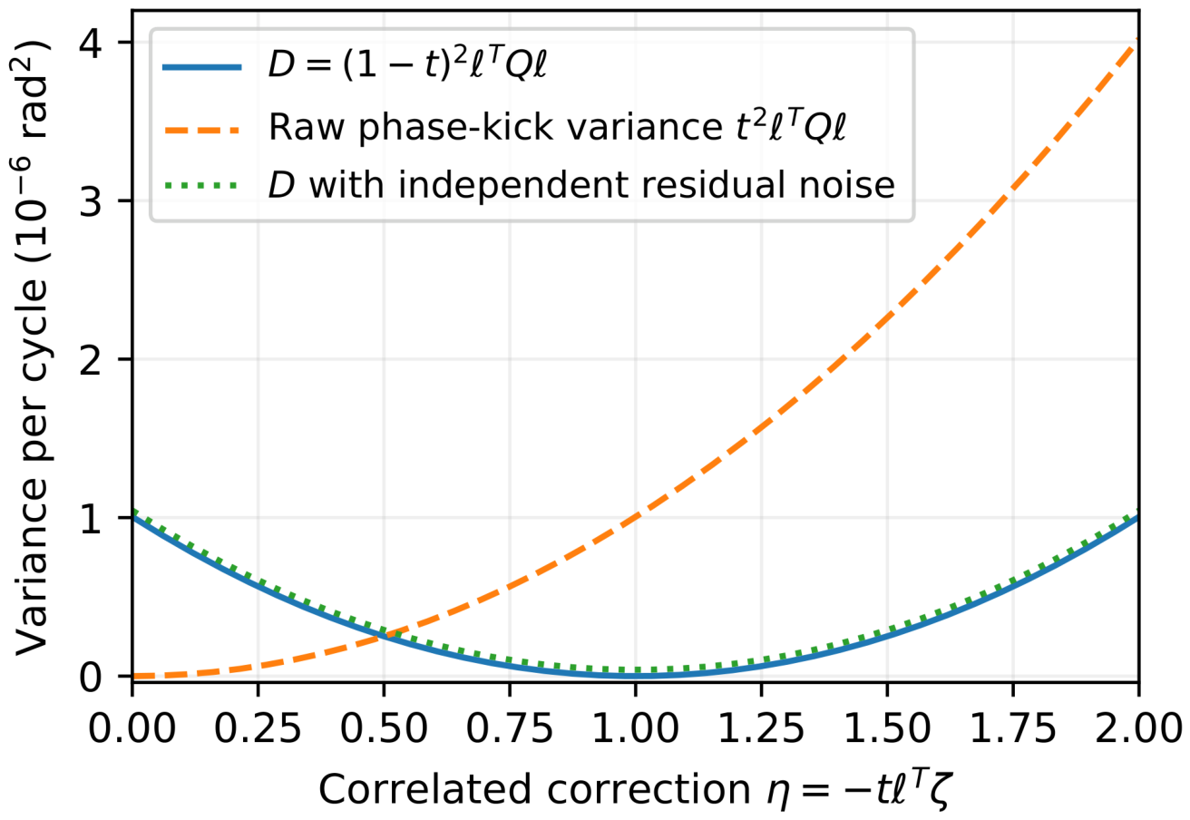
Figure 3. Event probabilities for ${\rho }_0=1+0.8cos2\chi$ and ${\xi }_0=0$, with the cell center following $n{\kappa }_{\mathrm{M}}$. Balanced counts remain at $1/2$ while quarter-cell counts approach $1/4$. The preparation channel is the one in Figure 1.

Figure 3. Event probabilities for ${\rho }_0=1+0.8cos2\chi$ and ${\xi }_0=0$, with the cell center following $n{\kappa }_{\mathrm{M}}$. Balanced counts remain at $1/2$ while quarter-cell counts approach $1/4$. The preparation channel is the one in Figure 1.

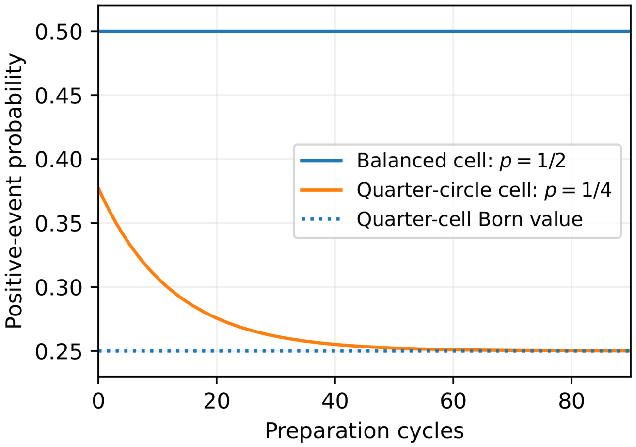
Figure 4. Relaxation from a fixed initial selector. The line is the exact first corrected-phase mode; markers show $50000$ independent synthetic trajectories with two-standard-error bars. The late-time mode falls below the sampling resolution, while Eq. (44) supplies its analytic preparation bound.

Figure 4. Relaxation from a fixed initial selector. The line is the exact first corrected-phase mode; markers show $50000$ independent synthetic trajectories with two-standard-error bars. The late-time mode falls below the sampling resolution, while Eq. (44) supplies its analytic preparation bound.

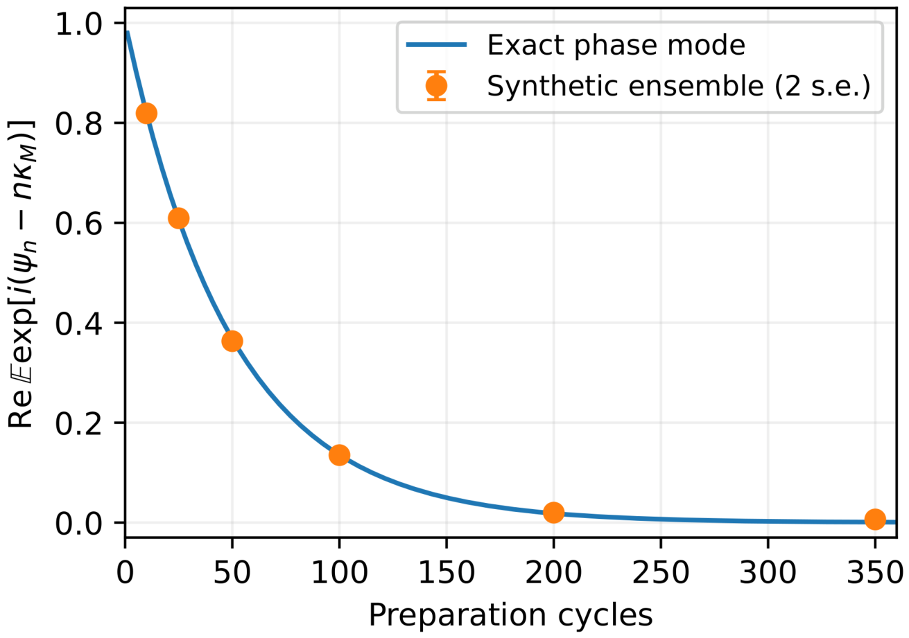
Table 1. Calculated preparation and readout channels. The response parameters $B,h,Q$ and the ideal phase ${\kappa }_{\mathrm{M}}$ are common. The final row gives the first cycle count at which the conditional bound is at most ${10}^{-3}$.

Quantity	Quiet readout	Preparation
${\sigma }_{\eta }$	0.002	0.200
D	$5.00507102\times {10}^{-6}$	$0.040001005$
$1/{\gamma }_1$ (cycles)	$399594.73$	$49.99874$
n for $\epsilon \left(v_n\right)\le {10}^{-3}$	2621816	329

Table 1. Calculated preparation and readout channels. The response parameters $B,h,Q$ and the ideal phase ${\kappa }_{\mathrm{M}}$ are common. The final row gives the first cycle count at which the conditional bound is at most ${10}^{-3}$.

Quantity	Quiet readout	Preparation
${\sigma }_{\eta }$	0.002	0.200
D	$5.00507102\times {10}^{-6}$	$0.040001005$
$1/{\gamma }_1$ (cycles)	$399594.73$	$49.99874$
n for $\epsilon \left(v_n\right)\le {10}^{-3}$	2621816	329

The same trajectories then enter the quiet channel for 408 cycles. Table 2 compares their event mismatch with the stationary law in Eq. (39). The geometric phase and the near return at lag 204 remain those of the original cycle. The simulation includes finite preparation error and sampling fluctuations; estimates at different lags use the same trajectory ensemble.

8. Finite-time Predictions for Implemented Instruments

The equilibrium and spectral laws refer to a complete cycle with independently determined response and reservoir parameters. Nonlinear response and selector-dependent readout recoil change its transition kernel. Their finite-time effect can be expressed in the same distance that controls the Born probabilities.

Let ${\mathsf{P}}_0$ be the affine kernel and $\mathsf{P}$ an implemented kernel on the full state $\omega =(\xi ,\chi )$. On a calibration domain K, suppose

$$\underset{\omega \in K}{sup}TV[\mathsf{P}(\omega ,·),{\mathsf{P}}_0(\omega ,·)]\le ϵ.$$

(45)

Write $p_{\mathrm{exit}}^{\left(0\right)}\left(n\right)$ for the probability that the reference state lies outside K before one of the first n transitions, including the initial state, and set

$${\Delta }_n=min\{1,nϵ+p_{\mathrm{exit}}^{\left(0\right)}\left(n\right)\}.$$

(46)

Proposition 5 

(Stability of the finite-time Born bound). For a common initial law μ,

$$TV(\mu {\mathsf{P}}^n,\mu {\mathsf{P}}_0^n)\le {\Delta }_n.$$

(47)

Whenever $S_n\succ 0$,

$$\begin{array}{cc}\hfill & TV[\mu {\mathsf{P}}^n,{\left(\mu {\mathsf{P}}^n\right)}_{\xi }\otimes {\mu }_{\mathrm{H}}]\hfill \\ \hfill & \le min\{1,\epsilon \left(v_n\right)+2{\Delta }_n\}.\hfill \end{array}$$

(48)

For K equal to the full state space, $p_{\mathrm{exit}}^{\left(0\right)}\left(n\right)=0$.

Proof. 

Couple the two processes while their common state lies in K. At each such step a maximal coupling separates them with conditional probability at most $ϵ$. The probability of separation by cycle n is bounded by $nϵ$ plus the reference exit probability, proving Eq. (47). Add and subtract the reference law and its response marginal times Haar measure. The middle distance is bounded by Theorem 2; the other two are bounded by ${\Delta }_n$, since marginalization contracts total variation. □

The implemented-kernel bound controls the response-averaged outcome distance from the same Born partition. The ideal Gaussian theorem gives the stronger bound at almost every resolved response.

A calibrated nonlinear mean remainder $\Delta \left(\omega \right)$ admits a direct comparison. For equal positive-definite innovation covariance $\mathsf{C}$, Gaussian relative entropy and Pinsker’s inequality give [11]

$$TV[\mathsf{P}(\omega ,·),{\mathsf{P}}_0(\omega ,·)]\le {\displaystyle \frac{1}{2}}\parallel {\mathsf{C}}^{-1/2}\Delta \left(\omega \right)\parallel .$$

(49)

Wrapping the phase contracts this distance. The remaining exit term is also calculable. For the reference process starting at ${\xi }_0=0$, the ellipsoid

$$K_R=\{\xi :{\xi }^{\mathsf{T}}{S}^{-1}\xi \le R^2\}\times \mathbb{T}$$

(50)

satisfies $p_{\mathrm{exit}}^{\left(0\right)}\left(n\right)\le nPr({\mathsf{X}}_d^2>R^2)$, where ${\mathsf{X}}_d^2$ has a chi-squared distribution. Appendix A proves this estimate. With $d=2$ and $R=8$, the bound over 350 preparation cycles is $4.44\times {10}^{-12}$. Equations (45)–(50) give separate, computable contributions from one-step approximation and finite-domain sampling.

An experimental comparison uses independent preparation ensembles at selected durations. A phase-sensitive preparation can produce a nonuniform selector law; in the ideal event model, conditioning on a balanced initial outcome produces a semicircle, with its response and charge disturbance carried by the initial joint distribution. Subsequent outcomes are retained. Response-resolved scans determine preparation harmonics, paired histories determine the corresponding fingerprints, and the measured joint kick covariance predicts both. Probe backaction enters the observation kernel [10]; causal-break protocols characterize retained external correlations [12]. The comparison is between complete population and correlation laws of the same identified instrument.

9. Discussion and Conclusion

The passage from an invariant Born ensemble to an attracting one is controlled by the phase fluctuation left after the response has been resolved. In the reservoir-coupled M-event cycle, this fluctuation has an exact coordinate representation. The stable response contributes a finite endpoint correction; the remaining innovation accumulates from cycle to cycle.

For a controllable Gaussian return, positive innovation variance is both necessary and sufficient for attraction from every initial joint law. Its limiting phase is Haar at each resolved response. The conditional Schur complement gives a finite-time Born bound, and a matching lower bound fixes the optimal preparation-uniform exponent to $D/2$. At zero innovation, correlated motion preserves a rotating phase label even when the individual coordinates fluctuate. The condition for equilibration is therefore carried by a covariance invariant, rather than by either raw noise amplitude alone.

Equilibrium formation and the M-event fingerprint share the same phase spectrum. A fixed channel attenuates a prepared harmonic and its matching two-time correlation by the same factor. Strong preparation followed by quieter readout separates their operational roles while retaining the original geometric phase. Variable-width event cells expose the harmonics needed to test this mechanism beyond balanced counts.

The physical–observation interface fixes the geometry of an event; the complete open cycle fixes how ensembles populate that geometry and how one event remains correlated with another. Their joint dynamics yields a single quantitative account of conditional Born equilibration and fingerprint decay. Equilibrium is a property of the ensemble. The fingerprint records the temporal structure that remains within it.

References

- Born, M. Zur Quantenmechanik der Stoßvorgänge. Z. Phys. 1926, 37, 863–867. [Google Scholar] [CrossRef]
- Valentini, A.; Westman, H. Dynamical origin of quantum probabilities. Proc. R. Soc. A 2005, 461, 253–272. [Google Scholar] [CrossRef]
- Hardel, V.; Hervieux, P.-A.; Manfredi, G. Relaxation to quantum equilibrium and the Born rule in Nelson’s stochastic dynamics. Found. Phys. 2023, 53, 89. [Google Scholar] [CrossRef]
- Meng, X. A categorical derivation of the dual-axis structure of observation. Preprints 2026, 202608.1298.v1. [Google Scholar]
- Meng, X. Deterministic Quantum Events on a Dual-Axis State Bundle: A Falsifiable Recurrence Test of Single-Event Continuity, author manuscript and accompanying Supplemental Material 2026. [CrossRef]
- X. Meng. Measurement Backaction, Selective Reset, and Stability of M-event Memory in a Physical–Observation Dual-Axis Theory author manuscript. 2026. [CrossRef]
- Demir, A.; Mehrotra, A.; Roychowdhury, J. Phase noise in oscillators: A unifying theory and numerical methods for characterization. IEEE Trans. Circuits Syst. I 2000, 47, 655–674. [Google Scholar] [CrossRef]
- Uhlenbeck, G. E.; Ornstein, L. S. On the theory of the Brownian motion. Phys. Rev. 1930, 36, 823–841. [Google Scholar] [CrossRef]
- Gordin, M. I. The central limit theorem for stationary processes. Dokl. Akad. Nauk SSSR 1969, 188, 739–741. [Google Scholar]
- Jacobs, K.; Steck, D. A. A straightforward introduction to continuous quantum measurement. Contemp. Phys. 2006, 47, 279–303. [Google Scholar] [CrossRef]
- van Erven, T.; Harremoës, P. Rényi divergence and Kullback–Leibler divergence. IEEE Trans. Inf. Theory 2014, 60, 3797–3820. [Google Scholar] [CrossRef]
- Pollock, F. A.; Rodríguez-Rosario, C.; Frauenheim, T.; Paternostro, M.; Modi, K. Operational Markov condition for quantum processes. Phys. Rev. Lett. 2018, 120, 040405. [Google Scholar] [CrossRef] [PubMed]